Abstract
Vegetation structure is a key component in assessing habitat quality for wildlife and carbon storage capacity of forests. Studies conducted at global scale demonstrate the increasing pressure of the agricultural frontier on tropical forest, endangering their continuity and biodiversity within. The Paraguayan Chaco has been identified as one of the regions with the highest rate of deforestation in South America. Uninterrupted deforestation activities over the last 30 years have resulted in the loss of 27% of its original cover. The present study focuses on the assessment of vegetation structure characteristics for the complete Paraguayan Chaco by fusing Sentinel-1, -2 and novel spaceborne Light Detection and Ranging (LiDAR) samples from the Global Ecosystem Dynamics Investigation (GEDI). The large study area (240,000 km2) calls for a workflow in the cloud computing environment of Google Earth Engine (GEE) which efficiently processes the multi-temporal and multi-sensor data sets for extrapolation in a tile-based random forest (RF) regression model. GEDI-derived attributes of vegetation structure are available since December 2019, opening novel research perspectives to assess vegetation structure composition in remote areas and at large-scale. Therefore, the combination of global mapping missions, such as Landsat and Sentinel, are predestined to be combined with GEDI data, in order to identify priority areas for nature conservation. Nevertheless, a comprehensive assessment of the vegetation structure of the Paraguayan Chaco has not been conducted yet. For that reason, the present methodology was developed to generate the first high-resolution maps (10 m) of canopy height, total canopy cover, Plant-Area-Index and Foliage-Height-Diversity-Index. The complex ecosystems of the Paraguayan Chaco ranging from arid to humid climates can be described by canopy height values from 1.8 to 17.6 m and canopy covers from sparse to dense (total canopy cover: 0 to 78.1%). Model accuracy according to median R2 amounts to 64.0% for canopy height, 61.4% for total canopy cover, 50.6% for Plant-Area-Index and 48.0% for Foliage-Height-Diversity-Index. The generated maps of vegetation structure should promote environmental-sound land use and conservation strategies in the Paraguayan Chaco, to meet the challenges of expanding agricultural fields and increasing demand of cattle ranching products, which are dominant drivers of tropical forest loss.
1. Introduction
The provision of ecosystem services of forests, such as carbon storage, habitats of rich biodiversity, and recreation are just a few key aspects of forests that foster sustainable future environmental conditions [1,2,3,4]. Since decades. constant deforestation activities have lead to the degradation of continuous forest, thus declining the provision of ecosystem services [5]. Most important changes are made to carbon emissions, since timber extraction and forest clearing amplify globally increasing atmospheric carbon concentrations on the one hand, and, on the other degrade carbon storage capacities of forests [3,6]. The forested areas of the Paraguayan Chaco have been continuously decreasing for decades, accounting to a total loss of 27% of the original cover from 1986 by 2012 [7]. One of the main drivers of the conversion of forests in artificial grasslands is cattle ranching, which is known for its high emissions and potentials to reduce emissions by intensification [8,9,10,11]. Therefore, there is increasing concern about the future and protection of the unique dry and humid forests of the Paraguayan Chaco.
For data processing and modelling, the cloud computing capabilities of Google Earth Engine (GEE) are used to efficiently handle the multi-temporal high-resolution data for the study area which spread over more than 240,000 km2 (2/3 of Germany). GEE has proven its capability for large-scale forest mapping and monitoring in numerous studies [12,13,14,15], including the high-resolution global maps of forest cover change for the 21st century by Hansen et al., 2021 [16]. By integrating the novel data sets of the full-waveform spaceborne LiDAR (Light Detection and Ranging) sensor (GEDI), the first high-resolution maps of canopy height, vegetation cover density and vertical foliage structure for the Paraguayan Chaco are generated. Therefore, the new knowledge of forest structure enables a more profound large-scale understanding of the Paraguayan Chaco’s forest ecosystems and provides additional information for forest conservation and the assessment of expected future forest loss.
For vegetation structure monitoring over large geographical areas, spaceborne LiDAR sensors are more practical and less expensive than terrestrial and airborne instruments. LiDAR sensors attached to satellites that are capable of capturing vegetation structure characteristics are scarce and limited to the NASA GLAS and ATLAS missions, i.e., the ICE-Sat instruments [17,18]. Characteristics of ICE-Sat, such as the discrete-return LiDAR signal, the laser wavelength, and the sensor’s name, highlight that the focus is on the measurement of ice properties. Therefore, the full-waveform LiDAR of GEDI, which is attached to the International Space Station (ISS) and has been operating since April 2019, samples vegetation structure characteristics near-globally (between 51.6° N and 51.6° S) and stands for new opportunities in the assessment of carbon and water cycling processes, biodiversity, and habitat modelling. Its specific characteristics, such as a sample footprint of 25 m, a laser wavelength in the near infrared (1064 nm), and a sampling scheme with eight ground-tracks, make the GEDI highly applicable for forestry-related research. Moreover, GEDI is characterized as a sampling mission, since vegetation structure attributes are measured in all tropical and sub-tropical forests. The benefits of GEDI’s sampling scheme are especially valuable in combination with globally operating sensors, such as Landsat and Sentinel, because their time-series data allow for spatiotemporal modelling of GEDI-derived vegetation structure [19]. An exemplary study of the aforementioned integration of sensors is the Global Forest Canopy Height Model from Potapov et al. 2021 [20], but monitoring approaches of GEDI and the derivation of attributes of forest structure using coarse-resolution sensors are further use-cases [21]. In addition, the study of Pereira-Pires et al., 2021 [22] presents the combination of GEDI and Sentinel-2 to model forest height accurately based on high-resolution optical data.
The present approach builds on aforementioned studies [20,21,22] by modelling vegetation structure characteristics based on fused Sentinel-1 and -2 data in a random forest regression model. Additionally, the high-resolution multi-temporal and multi-sensor data of Sentinel is fully processed in the cloud-computing geospatial analysis environment of GEE, which is why the presented workflow follows state-of-the-art remote sensing processing techniques [23,24]. The final data products are the first high-resolution maps (10 m) of canopy height, canopy cover density and vertical foliage structure complexity for the Paraguayan Chaco.
2. Materials and Methods
The chapter “2. Materials and Methods” is sub-divided into the chapters “Study Area”, giving an introduction to the Paraguayan Chaco, “Data Acqusition”, that explains Sentinel and GEDI data obtained, and “Data Processing and Methodology”, which presents the workflows for “Quality Filtering of Data”, “Calculation of Spectral Indices and Temporal-Spectral Metrics”, and “Modelling of Vegetation Structure and Validation”.
2.1. Study Area
The Paraguayan Chaco is located in the western part of Paraguay (Figure 1). Its forests belong to the Great American Chaco, which is the second largest region of continuous forest cover in South America after the Amazonian Forest [25]. It spreads over 240,000 km2, covering about 60% of Paraguay’s territory and contributing about 25% of Great American Chaco’s total area. The Paraguayan Chaco is divided into three political departments: Boquerón in the west is characterized by the most arid conditions, sandy soils and lowest annual precipitation rates. Alto Paraguay, which is located in the east, holds more humid conditions and more developed and clay-rich soils in its eastern areas due to higher annual precipitation rates and wetlands (Pantanal). The political department of Presidente Hayes presents the most dominantly humid conditions with a rather weak seasonality and mostly gleyic soils. Therefore, environmental conditions are especially diverse in the Paraguayan Chaco, since there are different influences of the semi-annual shift from dry to rainy season. Furthermore, soil fertility and water storing capacities differ between arid and humid climates [11].
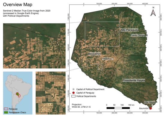
Figure 1.
Overview map of the study area depicted as Sentinel-2 median image of 2020. Deforested areas that have been converted to agricultural fields are characterized by their rectangular shape.
2.2. Data Acquisition
Sentinel data from the dry season 2019 (April to including September) was retrieved to model characteristics of vegetation structure for the Paraguayan Chaco. Data from the multi-spectral sensor Sentinel-2 in level 2A (Surface Reflectance) was processed together with C-Band Synthetic-Aperture-Radar (SAR) data from Sentinel-1 (Ground-Range-Detected) in GEE using the Python API. Both Sentinel data sets have a geometric resolution of 10 m which will be the target spatial resolution of the models.
Several attributes of vegetation structure have been obtained from the GEDI Release 2 data products “Elevation and Height Metrics” (L2A) [26] and “Canopy Cover and Vertical Profile Metrics” (L2B) [27]. GEDI data is stored as point geometries representing the centroid of the 25 m sample footprint. Vegetation structure attributes that were modelled are canopy height (95th percentile of the relative height metrics from GEDI L2A), total canopy cover (GEDI L2B), Plant-Area-Index (GEDI L2B) and Foliage-Height-Diversity-Index (GEDI L2B). According to the study of Potapov et al., 2021 [20], the 95th percentile of the canopy height metrics was selected since it presented higher correlations than the 100th percentile with airborne LiDAR. In addition, total canopy cover, defined as the vertical projection of canopy material per area [28], and Plant-Area-Index are vegetation structure attributes that describe the density of canopy cover material [29]. The Foliage-Height-Diversity-Index, also known as Shannon’s diversity index, focuses on the assessment of vertical vegetation structure complexity [30].
2.3. Data Processing and Methodology
In the following, the data processing workflow is explained in more detail, comprising quality filtering, derivation of spectral indices, calculation of temporal-spectral metrics, modelling and model validation. Aforementioned processing steps are displayed in Figure 2.
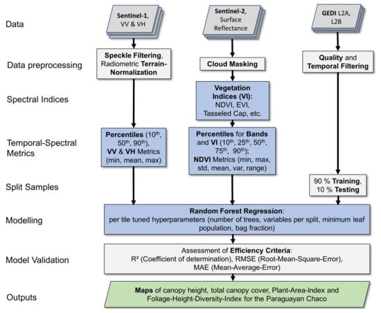
Figure 2.
Workflow diagram depicting data preprocessing steps of Sentinel-1, -2 and Global Ecosystem Dynamics Investigation (GEDI).
For data processing several computing resources have been used. Downloading multi-temporal GEDI data was conducted using a virtual machine with 32 GB RAM (processing time about five days). Quality and temporal filtering of GEDI, but also preparing the GEDI data for the tile-based modelling approach, was conducted on a local computer with 16 GB RAM (processing time about one day). The cloud-computing environment of GEE was used to access and preprocess Sentinel-1 and -2 for modelling (processing time about three days). The preparation of the GEE exports for visualization and the model accuracy assessment was conducted on the aforementioned local computer (processing time about 2 days).
2.3.1. Quality Filtering of Data
Sentinel-1 data was filtered to single co-polarization in vertical transmit and vertical receive (VV) and the dual-band cross-polarization in vertical transmit and horizontal receive (VH). Preprocessing steps include speckle filtering and radiometric terrain normalization for analysis-ready Sentinel-1 [31] and filtering for “Cloudy Pixel Percentage” lower than 30% and cloud masking for Sentinel-2. In total, 125 Sentinel-1 and 1029 Sentinel-2 scenes were obtained for analysis.
GEDI data in level L2A and L2B was quality-filtered according to the Algorithm Theoretical Basis Document [28] to remove degraded and low sensitivity shots. In addition GEDI data was temporally filtered to match the period of the Sentinel data (June to including September 2019).
2.3.2. Calculation of Spectral Indices and Temporal-Spectral Metrics
Several spectral indices for Sentinel-2 have been calculated as additional vegetation structure proxies to the spectral information of Sentinel-1 and -2. Spectral indices range from basic vegetation indices (VI) (e.g., Difference-Vegetation-Index (DVI) [32,33], Normalized-Difference-Vegetation-Index (NDVI) [34]) over indices that consider atmospheric effects (e.g., Atmospherically-Resistant-Vegetation-Index (ARVI2) [35]) to spectral transformations (e.g., tasseled cap [36,37], Enhanced-Vegetation-Index (EVI) [38]). Table 1 displays calculated vegetation indices.

Table 1.
Table of vegetation indices (VI) that were calculated for temporal-spectral metrics derivation.
According to Franklin et al., 2015 [45], Hansen et al., 2014 [46], Müller et al., 2016 [47] and Potapov et al., 2021 [20], to aggregate multi-temporal satellite data, a reliable approach is the calculation of temporal-spectral metrics to account for gaps and temporal variability in the data series, e.g., due to atmospheric interference (clouds, cloud shadows) [20,45,46,47]. Additionally, the integration of multi-temporal data is essential to achieve a complete coverage for large-scale study areas, such as the Paraguayan Chaco [48]. For Sentinel-1, several percentiles (10th, 50th, 90th) and minimum, mean and maximum metrics were calculated for both polarizations. The temporal-spectral metrics for Sentinel-2 consist of percentile metrics for the bands and VI (10th, 25th, 50th, 75th, 90th). In addition, a NDVI metrics (minimum, maximum, standard deviation, mean, variance, range) was calculated to specifically capture phenological variations. In total, 138 spectral features of Sentinel-1 and -2 serve as input for modelling characteristics of vegetation structure.
In addition to the spectral information of Sentinel-1 and -2, elevation data from TanDEM-X in 12 m [49,50] was added to the model stack.
2.3.3. Modelling of Vegetation Structure and Validation
To model the Paraguayan Chaco’s vegetation structure, the study area was subdivided into 89 tiles (0.5° × 0.5°) to facilitate parallel processing and avoid computational limits in GEE. For each attribute of vegetation structure, a random forest regression model was set up with tuned hyperparameters.
A random forest (RF) model is a machine-learning ensemble technique that has proven its popularity in remote sensing applications due to high accuracy and performance [51,52]. An RF model applies bootstrapping and aggregation on a user-defined number of decision trees which can lead to a substantial increase in accuracy due to the reduction in variance of predictions to observations [53,54]. To improve the learning of the RF model, hyperparameters, such as number of trees, minimum leaf population, variables per split and bag fraction can be optimized using sensitivity analysis. By varying the values of each hyperparameter, the model accuracy can increase, which enables a better understanding of the algorithm and its sensitivity to parameter changes [55,56]. The sensitivity analysis was conducted similar to the study of Janalipour et al., 2017 [57]. In GEE, the RF model output can be set to regression to model continuous variables and apply an averaging of the predictions from all decision trees, opposing to a RF classification model where predictions are aggregated based on majority voting [58]. In total, about 700,000 quality-filtered GEDI samples have been used in model training and validation of each attribute of vegetation structure.
According to the study of Potapov et al., 2021 [20], the set of GEDI samples was randomly split before modelling in a collection of training samples (90%) and testing samples (10%) for model validation. In addition, to match the ratio of samples/km2 of the studies from Potapov et al., 2021 (2.6 samples/km2) [20] and Rishmawi et al., 2021 (3.4 samples/km2) [21], 8000 samples (3 samples/km2) have been randomly selected from a pool of more than 15,000 samples per tile-model. Due to the high number of samples, the aforementioned sampling workflow results in a spatially and temporal balanced data set. Only in some western and eastern tile-models, there are rather non heterogeneously-scattered samples for the tile-models because GEDI samples do not cover the full temporal range, e.g., observations are only of one month. The testing samples which are independent from modelling, are used to calculate several model efficiency criteria, such as the mean-average-error (MAE), coefficient of determination (R2) and root-mean-square-error (RMSE).
3. Results
The results chapter is divided into the sub-chapters “Error assessment”, that explains modelling uncertainties, “Model Sensitivity Analysis”, which assesses influences of hyperparameter tuning on the RF models performance, and “Modelled Vegetation Structure Attributes”, that presents the modelled results as maps.
3.1. Error Assessment
To assess the statistical uncertainty of modelled canopy height, total canopy cover, Plant-Area-Index and FHDI, the independent set of GEDI samples (observations) was compared to model predictions by calculating the mean-average-error (MAE), coefficient of determination (R2) and root-mean-square-error (RMSE). Since modelling was conducted by implementing a tile-based approach, for each modelled tile and GEDI attribute, the error criteria were calculated and aggregated as mean and median values in Table 2. The highest model accuracy was achieved, according to the non-scale-dependent criteria R2, for the canopy height (mean: 60.0%, median: 64.0%) and total canopy cover models (mean: 61.8%, median: 61.4%). For modelled canopy height, MAE amounts to 1.1 m and RMSE to 1.6 m. The statistical uncertainty of modelled total canopy cover has an average MAE value of 6.0 to 6.2% and average RMSE of 9.1 to 9.4%. Modelled Plant-Area-Index and FHDI present identical errors for the scale-dependent criteria MAE (0.2) and RMSE (0.3). According to R2, modelled Plant-Area-Index is slightly higher (mean: 50.1%, median: 50.6%) than FHDI (mean: 47.4%, median: 48.0%).
Table 2.
Table of model errors: MAE (Mean-Average-Error), coefficient of determination (R2) and RMSE (Root-Mean-Square-Error). Median and mean values per error criteria have been calculated from all modelled tiles.
The assessment of differences (Figure A3) between modelled canopy height (rh95) and observations (GEDI validation samples) presents lowest relative errors in the range of average canopy heights of the Paraguayan Chaco (4 to 6 m). Furthermore, there is a pattern of model underestimation (2 to 4 m) to strong model overestimation (12 to 16 m).
Model accuracy of canopy height is similar to that of the Landsat based Global Forest Canopy Height model of Potapov et al. 2021 [20] and canopy height models of Pereira-Pires et al., 2021 [22], using Sentinel-2 spectral features.
3.2. Model Sensitivity Analysis
The sensitivity analysis of model accuracy (estimated using R2 values) highlights that varying the values of each hyperparameter, e.g., number of trees from 50 to 250 trees, influences model accuracy (56.7% to 57.5%) (Figure 3, upper left). In comparison to the hyperparameter tuning for number of trees (optimum at about 250 trees), the other hyperparameters present stronger differences in R2 when testing several values. The sensitivity analysis reveals for the minimum leaf population that not trimming the decision trees, i.e., allowing for low minimum leaf populations, results in highest model accuracy (up to 57%) (Figure 3, upper right). In comparison to the negative correlation between R2 and minimum leaf population, the hyperparameters variables per split and bag fraction are holding positive correlations with model accuracy. Therefore, an increased number of variables per split and elevated fractions of samples for model training, improve model accuracy (Figure 3, lower left and right).
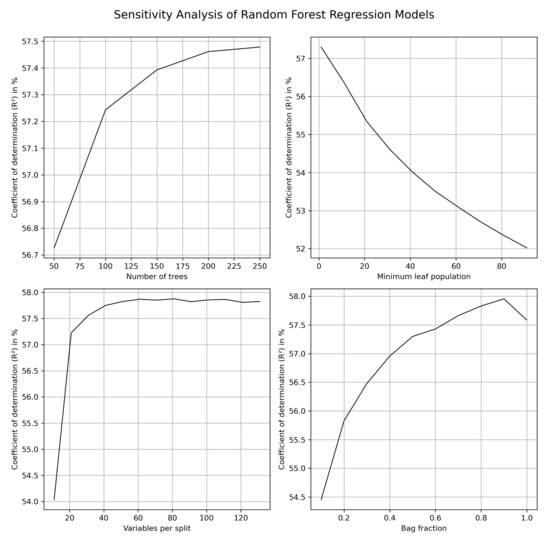
Figure 3.
The plots depict the sensitivity analysis of all random forest regression models according to the hyperparameters number of trees (upper left), minimum leaf population (upper right), variables per split (lower left) and fraction used for model training (lower right). The coefficient of determination (R2) serves as parameter to assess model accuracy. Findings are that an increased number of trees, low minimum leaf populations, high number of variables per split, and an increased fraction of samples used for model training, improve model accuracy according to R2.
To sum up the findings of the sensitivity analysis, tuned hyperparameters to the level of highest model accuracy according to R2, improve the model performance. Combining all tuned hyperparameters in the model, results in the model accuracies presented in Table 2.
3.3. Modelled Vegetation Structure Attributes
Modelled canopy height ranges from 1.8 to 17.6 m, with a mean value of about 5.3 m for the Paraguayan Chaco. There are strong differences in canopy heights between agricultural fields, which present values lower than 2 m and are characterized by their rectangular shape (Figure 4, upper and lower sub-map), and clusters of elevated canopy heights (greater than 14 m) in the north-east and south-east. The high geometric resolution of 10 m allows the identification of road networks (middle sub-map) and of characteristics of agricultural fields such as forest islands and wind barriers (lower sub-map). Furthermore, the lowest modelled canopy heights outside agricultural fields (≈4 m) are found in the Ecoregion Médanos which is located in the north-west and holds the most arid, desert-like climate of the Paraguayan Chaco. The more humid regions (south-east) present linear structures of increased canopy heights (greater than 9 m) along major rivers.
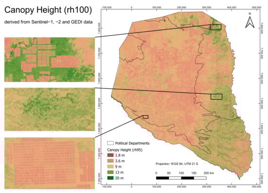
Figure 4.
Modelled canopy height (rh95) for the Paraguayan Chaco.
Modelled total canopy cover is presented in Figure 5 with canopy cover densities ranging from about 0% (no canopy cover present) to 78.1% (dense to closed canopy covers). The mean total canopy cover density amounts to 19.5%, which highlights the overall rather sparse levels of canopy cover conditions in the Paraguayan Chaco. Small-scale differences of total canopy cover are present in agricultural fields (upper and lower sub-map), since agricultural fields are characterized by no canopy cover present (about 0%), whereas the aforementioned wind barriers between agricultural fields and forest islands hold higher total canopy cover densities (≈20%). In addition, there are also small-scale differences (middle sub-map) between riparian areas (elevated total canopy cover of about 70%) and the open grasslands (total canopy cover lower than 20%) which can be identified in the south-eastern parts of Figure 5, middle sub-map. An overall observation similar to modelled canopy height (Figure 4), is the gradual increase of total canopy cover from the north-west to the east and south-east when omitting agricultural fields. This finding corresponds to the precipitation rates of the Paraguayan Chaco.
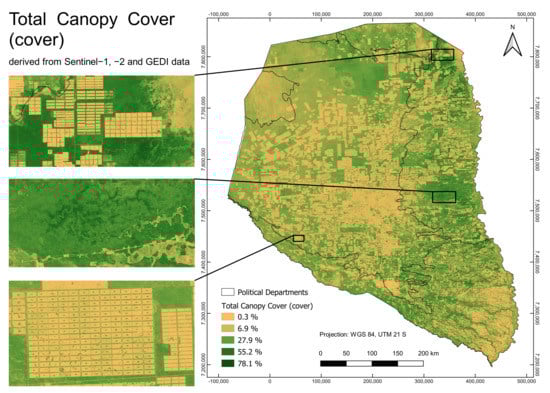
Figure 5.
Modelled total canopy cover (cover) for the Paraguayan Chaco.
The map of modelled Plant-Area-Index (Figure 6), holds information similar to total canopy cover, since both attributes describe canopy coverage densities. Values range from 0 (no plant per area) to 4 (high plant area density) and present aforementioned patterns of agricultural fields (Plant-Area-Index ≈ 0) that dominate in the center, western and north-eastern regions of the Paraguayan Chaco. The mean Plant-Area-Index for the Paraguayan Chaco amounts to 0.51, describing rather low overall cover densities. The aforementioned longitudinal pattern of elevated canopy heights and total canopy covers towards the eastern parts, is also identifiable for Plant-Area-Index.
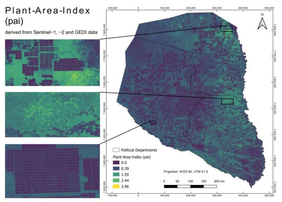
Figure 6.
Modelled Plant-Area-Index (pai) for the Paraguayan Chaco.
Modelled Foliage-Height-Diversity-Index (FHDI) in Figure 7 differentiates between simple (FHDI ≈ 0.7) and complex vertical foliage structures that consist of multiple canopy layers (FHDI ≈ 2.8). The mean value of FHDI for the Paraguayan Chaco amounts to 1.79, which describes medium complex foliage structures. The spatial patterns of FHDI match the results of modelled canopy height and cover density, with the least complex foliage structures in agricultural fields (FHDI ≈ 0.7) and elevated FHDI (≈2.8) in the more humid regions of the Paraguayan Chaco in the north-east and south-east.
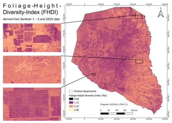
Figure 7.
Modelled Foliage-Height-Diversity-Index (FHDI) for the Paraguayan Chaco.
4. Discussion
The cloud-processing capabilities of GEE greatly enabled the methodological development and implementation of the present study. Multi-temporal and multi-sensor data was efficiently processed to accurately model vegetation structure characteristics based on Sentinel and GEDI data for the Paraguayan Chaco. To the authors’ knowledge, the present study describes the first assessment of vegetation structure obtained from high-resolution remote sensing imagery for the Paraguayan Chaco. Furthermore, the present approach highlights the applicability and benefits of sensor fusion for vegetation modelling and the derivation of large-scale key attributes of vegetation structure, valuable information for the improvement of biomass and emission models [59,60]. In addition, this approach promotes reproducible research in the field of remote sensing, which is often hindered by the necessity of processing high-resolution and multi-temporal satellite data for large study areas, since the presented workflow is independent from institutional cluster-computing infrastructures. In addition, the GEE data catalog provides various kinds of satellite data in high processing levels, freeing up more time for analysis since the analysis is brought to the data in a cloud-computing environment.
By accessing the data catalogue of GEE, which holds high-level products of Sentinel-1 and -2, data preprocessing was limited to speckle filtering and radiometric terrain normalization for Sentinel-1 and cloud filtering and masking for Sentinel-2. Furthermore, the state-of-the-art algorithms in GEE allow for efficient and rapid calculation of spectral indices and temporal-spectral metrics for the complete Paraguayan Chaco. Therefore, in this work, several spectral features suggested in the study of Pereira-Pires et al., 2021 [22] have been combined for vegetation structure modelling in random forest regression models. Since the presented methodological framework is implemented in the cloud-processing capabilities of GEE, only final data products, such as the rasters of modelled vegetation structure and model errors, are exported on the local computer. The limitation to fully implementing the analysis in GEE is the lack of GEDI data, which is not part of the GEE data catalogue yet. Therefore, preprocessing of GEDI was conducted in a local Python environment to apply quality and temporal filtering for about 1.8 million LiDAR shots. Preprocessed GEDI data was in the following imported as GEE asset for cloud computing.
To estimate the contribution of spectral features to the model performance, variable importances of the RF model have been analyzed (Figure A1 and Figure A2). Calculated percentiles of the Sentinel-2 red edge bands present for all attributes of vegetation structure high importances. Those bands, which are unique to the Sentinel-2 sensor, are capable to detect chlorophyll and nitrogen contents of vegetation, highlighting the added spectral value, e.g., in comparison to Landsat data without bands in the red edge spectra [61,62]. Furthermore, the Sentinel-2 SWIR bands, specifically the 90th percentile of normalized-difference between the SWIR1 and SWIR2 band, are of special importance for all modelled GEDI attributes. SWIR bands are characterized by the ability to discriminate the moisture content of soil and vegetation [63]. The increased importance of tasseled cap brightness for all models of vegetation structure might be due to its information on soil albedo, e.g., dry and wet soils [36,64]. Most important spectral features of Sentinel-1 are the 10th percentiles of the VV and VH polarization. Sentinel-1 features might improve the model due to its capabilities to detect permanent water bodies (rivers, riparian areas) and high biomass levels [65]. To sum up, the presented methodology, which bases on the fusion of Sentinel-1 and -2, benefits from complementary sensor characteristics to assess various important proxies for modelling GEDI-derived attributes of vegetation structure.
The dry season period (June to including September) was selected due to increased cloud coverage in the rainy season (November to including April) [11]. Acquiring dry season data only for Sentinel and GEDI, goes along with the fact that vegetation structure is modelled at a phenological state of rather low canopy cover densities and little vegetation growth, compared to the rainy season. In addition, since multi-temporal Sentinel data is processed for the Paraguayan Chaco, it needs to be assumed that some locations of GEDI samples have undergone significant changes in their spectral information due to changes in land cover. Therefore, a large variety of spectral indices and bands was combined in temporal-spectral metrics to limit influences of significant spectral changes on modelling [20]. In addition, the high number of GEDI samples might further reduce the effect of significant spectral changes [19].
Modelled vegetation structure attributes present positive spatial correlations that follow the climate conditions of the Paraguayan Chaco: the more humid regions in the east present the highest canopy heights and most dense vegetation at elevated vertical complexity, whereas the most arid regions in the north-west are characterized by low canopy heights with open to sparse canopy cover densities. Agricultural fields can be easily detected due to abrupt changes of vegetation structure, i.e., lower canopy heights and more sparse canopy covers in agricultural fields in comparison to surrounding non-deforested vegetation. The integration of GEDI-based vegetation height data in combination with Sentinel-1 has also improved the binary classifications of forests and non-forested areas in tropical wetland regions as presented in the study of Verhelst et al., 2021 [66]. Furthermore, the middle sub-maps of Figure 4, Figure 5, Figure 6 and Figure 7 present elevated values for the vegetation structure attributes in wetland and riparian areas, which are characterized by linear spatial patterns. Along major rivers in the southern part of the Paraguayan Chaco, riparian areas highlight that the availability of water, in combination with soils that are prone to flooding, promote increased vegetation height and density. Although, to the knowledge of the authors, that there is no research about forest structure based on remote sensing techniques for the Paraguayan Chaco, the study of Akay et al., 2012 [67] for western Oregon (USA) describes similar characteristics of riparian forests as modelled for the Paraguayan Chaco in the present study: based on airborne LiDAR, elevated canopy cover densities and increased tree heights have been detected in riparian forests, highlighting the particularly favorable habitat conditions for wildlife [68].
Higher model accuracies might be hindered on the one hand by the 25 m GEDI footprint, which is a signal of mixed vegetation structure, that is on the other hand represented by a single Sentinel pixel (10 m). In other words, only a fraction of the GEDI samples is captured by the model predictors, limiting the spectral representation of model predictors. Furthermore, the studies of Dorado-Roda et al., 2021 (european mediterranean forests) [69] and Quirós et al., 2021 (Southwest Spain) [70] highlight that there are certain limitations to GEDI-derived canopy height estimates and georeference. But limitations in GEDI-derived canopy height are specifically related to highly multilayered forest structures [69], which are only a minor proportion of the forests of the Paraguayan Chaco (Figure 7). Another important point about the presented study is that there are lower numbers of GEDI samples available in the western and eastern parts of the Paraguayan Chaco, and therefore less spatially and temporally balanced sample sets. Those models might not be as accurate as models with spatially and temporally balanced sample sets, since on the one hand, not the complete range of vegetation structure is sampled due to a heterogeneous sample scattering. On the other, the availability of samples from a limited period, e.g., only one month, only trains the model for a certain phenological state of the dry season. Nevertheless, modelled canopy height of the present study is similar to the Landsat-based canopy height model of Potapov et al., 2021 [20] in terms of accuracy and according to mean (difference: 0.3 m) and median values (difference: 0.1 m) for the forests of the Paraguayan Chaco.
Differences in model accuracy between vegetation structure characteristics can be interpreted as the difference in Sentinel’s capability to represent various characteristics of vegetation structure. Therefore, canopy height and total canopy cover, which present the highest R2 accuracies, can be considered as more direct proxies of the multi-spectral and radar signals than Plant-Area-Index and FHDI. Especially FHDI aggregates vertical and horizontal information of vegetation structures, which can hardly be represented by optical information of Sentinel-2.
Research that is beyond the scope of this paper, but could be addressed in future work, is a statistical assessment of correlations between modelled vegetation structure and environmental conditions, such as temperature, precipitation, land cover, and soil types, to better understand spatial patterns of vegetation structure. Furthermore, the combination of information on forest cover and forest structure enables a more comprehensive evaluation of changes in ecosystem services and functioning due to deforestation. In addition, upcoming data of GEDI (nominal lifetime of 2 years) will allow for multi-temporal monitoring of vegetation structure, e.g., to detect degraded forests due to differences in canopy height. In this context, forest canopy height time-series profiles have been modelled based on GEDI samples and Landsat time-series data in the study of Potapov et al., 2021 [20]. Therefore, different land use practices have been detected, such as selective logging, clearcuts and plantations.
5. Conclusions
This paper presents a cloud-based vegetation structure modelling approach in GEE to derive canopy height, total canopy cover, Plant-Area-Index and Foliage-Height-Diversity-Index for the Paraguayan Chaco. The advantages of GEE to rapidly process large satellite data sets, in combination with the provision of a rich data catalogue, facilitates the presented methodology. Therefore, high-resolution multi-temporal data from Sentinel-1 and -2 was fused with GEDI data to model vegetation structure in tile-based random forest regression models.
The main results are the first high-resolution maps of vegetation structure attributes for the complete Paraguayan Chaco. There are strong differences in vegetation structure within the Paraguayan Chaco due to diverse environmental conditions that range from arid to humid climates, i.e., desert-like conditions to riparian and wetland areas. Overall, vegetation is rather low (mean canopy height: 5.3 m) and rather sparse (mean total canopy cover: 19.5%).
The novel generated data sets of vegetation structure from high-resolution spaceborne LiDAR samples should support strategies to halt deforestation that has been going on for decades in the Paraguayan Chaco. The developed methodology allows for the spatiotemporal modelling of vegetation structure almost globally (restricted by the coverage of GEDI). In addition, high-resolution global products of forest structure might improve carbon emission and biomass models to determine global carbon balances more accurately to further promote global emission reduction initiatives.
Author Contributions
Conceptualization, P.K. and E.D.P.; Methodology, A.H. and P.K.; Software, P.K.; Validation, P.K. and E.D.P.; Formal analysis, P.K.; Investigation, P.K.; Resources, E.D.P.; Data curation, A.H.; Writing—original draft preparation, P.K.; Writing—review and editing, P.K. and E.D.P.; Visualization, P.K.; Supervision, E.D.P.; Project administration, E.D.P.; Funding acquisition, E.D.P. All authors have read and agreed to the published version of the manuscript.
Funding
This work was conducted under the project GeoForPy ‘Understanding forest cover for biodiversity conservation in the Paraguayan Chaco’ executed by the German Aerospace Center (DLR) and supported by funds of the Federal Ministry of Food and Agriculture (BMEL) based on a decision of the Parliament of the Federal Republic of Germany via the Federal Office for Agriculture and Food (BLE).
Institutional Review Board Statement
Not applicable.
Informed Consent Statement
Not applicable.
Data Availability Statement
Sentinel-1 (Ground-Range-Detected) and -2 (Surface Reflectance) data was obtained from the GEE data catalog. GEDI data in Level 2A and 2B was downloaded using the GEDI Finder. To access the rasters of modelled vegetation structure (10 m), please contact the corresponding author.
Conflicts of Interest
The authors declare no conflict of interest.
Abbreviations
The following abbreviations are used in this manuscript:
| cover | total canopy cover |
| DVI | Difference-Vegetation-Index |
| EVI | Enhanced-Vegetation-Index |
| FHDI | Foliage-Height-Diversity-Index |
| GEE | Google Earth Engine |
| GEDI | Global Ecosystem Dynamics Investigation |
| GNDVI | Green-Normalized-Difference-Vegetation-Index |
| IPVI | Infrared-Percentage-Vegetation-Index |
| ISS | Internation Space Station |
| LCI | Leaf-Chlorophyll-Index (LCI) |
| LiDAR | Light Detection and Ranging |
| MAE | mean-average-error |
| ND | Normalized difference |
| NDMI | Normalized-Difference-Moisture-Index |
| NDVI | Normalized-Difference-Vegetation-Index |
| NDWI | Modified Normalized-Difference-Water-Index |
| p | percentile |
| pai | Plant-Area-Index |
| rh95 | canopy height (95th percentile) |
| R2 | Coefficient of determination |
| RE | Red Edge |
| RF | Random Forest |
| RMSE | root-mean-square-error |
| SAR | Synthetic-Aperture-Radar |
| SWIR | Shortwave infrared |
| VH | vertical transmit, horizontal receive |
| VI | Vegetation-Index |
| VV | vertical transmit, vertical receive |
Appendix A
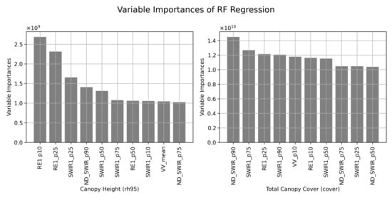
Figure A1.
RF Regression: ten most important variables for canopy height (rh95) and total canopy cover (cover). Abbreviations: ND = Normalized difference, p = percentile, RE = Red Edge, SWIR = Shortwave infrared, VV = vertical transmit, vertical receive polarization.
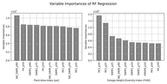
Figure A2.
RF Regression: ten most important variables for Plant-Area-Index (pai) and Foliage-Height-Diversity-Index (FHDI). Abbreviations: ND = Normalized difference, p = percentile, RE = Red Edge, SWIR = Shortwave infrared, VH = vertical transmit, horizontal receive polarization, VV = vertical transmit, vertical receive polarization.
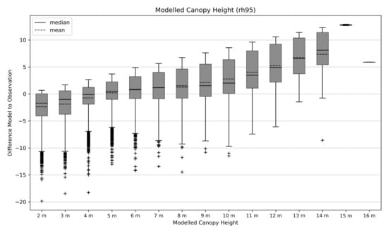
Figure A3.
Statistical analysis of modelled canopy heights errors (difference model to observation (GEDI validation samples)). The boxplots depict lowest errors at canopy heights of 4 to 6 m (average modelled canopy heights of the Paraguayan Chaco). In addition, there is a trend of underestimation (2 to 4 m) to strong overestimation (12 to 16 m) in terms of modelled canopy height.
References
- Achard, F.; Hansen, M.C. Global Forest Monitoring from Earth Observation; CRC Press: Boca Raton, FL, USA, 2016. [Google Scholar] [CrossRef]
- Houghton, R.A. Aboveground Forest Biomass and the Global Carbon Balance. Glob. Chang. Biol. 2005, 11, 945–958. [Google Scholar] [CrossRef]
- Mittermeier, R.A.; Turner, W.R.; Larsen, F.W.; Brooks, T.M.; Gascon, C. Global biodiversity conservation: The critical role of hotspots. In Biodiversity Hotspots; Springer: Berlin/Heidelberg, Germany, 2011; pp. 3–22. [Google Scholar]
- Pugh, T.A.M.; Lindeskog, M.; Smith, B.; Poulter, B.; Arneth, A.; Haverd, V.; Calle, L. Role of forest regrowth in global carbon sink dynamics. Proc. Natl. Acad. Sci. USA 2019, 116, 4382–4387. [Google Scholar] [CrossRef] [PubMed] [Green Version]
- DeFries, R. Why forest monitoring matters for people and the planet. Glob. For. Monit. Earth Obs. 2013, 8, 1–4. [Google Scholar]
- Brinck, K.; Fischer, R.; Groeneveld, J.; Lehmann, S.; Paula, M.D.D.; Pütz, S.; Sexton, J.O.; Song, D.; Huth, A. High resolution analysis of tropical forest fragmentation and its impact on the global carbon cycle. Nat. Commun. 2017, 8. [Google Scholar] [CrossRef] [Green Version]
- Baumann, M.; Israel, C.; Piquer-Rodríguez, M.; Gavier-Pizarro, G.; Volante, J.N.; Kuemmerle, T. Deforestation and cattle expansion in the Paraguayan Chaco 1987–2012. Reg. Environ. Chang. 2017, 17, 1179–1191. [Google Scholar] [CrossRef]
- Bustamante, M.M.C.; Nobre, C.A.; Smeraldi, R.; Aguiar, A.P.D.; Barioni, L.G.; Ferreira, L.G.; Longo, K.; May, P.; Pinto, A.S.; Ometto, J.P.H.B. Estimating greenhouse gas emissions from cattle raising in Brazil. Clim. Chang. 2012, 115, 559–577. [Google Scholar] [CrossRef]
- Bogaerts, M.; Cirhigiri, L.; Robinson, I.; Rodkin, M.; Hajjar, R.; Junior, C.C.; Newton, P. Climate change mitigation through intensified pasture management: Estimating greenhouse gas emissions on cattle farms in the Brazilian Amazon. J. Clean. Prod. 2017, 162, 1539–1550. [Google Scholar] [CrossRef]
- Cohn, A.S.; Mosnier, A.; Havlik, P.; Valin, H.; Herrero, M.; Schmid, E.; O’Hare, M.; Obersteiner, M. Cattle ranching intensification in Brazil can reduce global greenhouse gas emissions by sparing land from deforestation. Proc. Natl. Acad. Sci. USA 2014, 111, 7236–7241. [Google Scholar] [CrossRef] [PubMed] [Green Version]
- Gill, E.A.; Ponte, E.D.; Insfrán, K.P.; González, L.R. Atlas of the Paraguayan Chaco. 2020. Available online: https://www.dlr.de/eoc/en/PortalData/60/Resources/dokumente/2_dfd_la/Atlas_Chaco_Digital_Gill_Da_Ponte_et_al.pdf (accessed on 1 June 2021).
- Brovelli, M.A.; Sun, Y.; Yordanov, V. Monitoring Forest Change in the Amazon Using Multi-Temporal Remote Sensing Data and Machine Learning Classification on Google Earth Engine. ISPRS Int. J. Geo-Inf. 2020, 9, 580. [Google Scholar] [CrossRef]
- Chen, B.; Xiao, X.; Li, X.; Pan, L.; Doughty, R.; Ma, J.; Dong, J.; Qin, Y.; Zhao, B.; Wu, Z.; et al. A mangrove forest map of China in 2015: Analysis of time series Landsat 7/8 and Sentinel-1A imagery in Google Earth Engine cloud computing platform. ISPRS J. Photogramm. Remote Sens. 2017, 131, 104–120. [Google Scholar] [CrossRef]
- Chen, S.; Woodcock, C.E.; Bullock, E.L.; Arévalo, P.; Torchinava, P.; Peng, S.; Olofsson, P. Monitoring temperate forest degradation on Google Earth Engine using Landsat time series analysis. Remote Sens. Environ. 2021, 265, 112648. [Google Scholar] [CrossRef]
- Koskinen, J.; Leinonen, U.; Vollrath, A.; Ortmann, A.; Lindquist, E.; d’Annunzio, R.; Pekkarinen, A.; Käyhkö, N. Participatory mapping of forest plantations with Open Foris and Google Earth Engine. ISPRS J. Photogramm. Remote Sens. 2019, 148, 63–74. [Google Scholar] [CrossRef]
- Hansen, M.C.; Potapov, P.V.; Moore, R.; Hancher, M.; Turubanova, S.A.; Tyukavina, A.; Thau, D.; Stehman, S.V.; Goetz, S.J.; Loveland, T.R.; et al. High-Resolution Global Maps of 21st-Century Forest Cover Change. Science 2013, 342, 850–853. [Google Scholar] [CrossRef] [PubMed] [Green Version]
- Neuenschwander, A.L.; Magruder, L.A. Canopy and Terrain Height Retrievals with ICESat-2: A First Look. Remote Sens. 2019, 11, 1721. [Google Scholar] [CrossRef] [Green Version]
- Simard, M.; Pinto, N.; Fisher, J.B.; Baccini, A. Mapping forest canopy height globally with spaceborne lidar. J. Geophys. Res. 2011, 116. [Google Scholar] [CrossRef] [Green Version]
- Dubayah, R.; Blair, J.B.; Goetz, S.; Fatoyinbo, L.; Hansen, M.; Healey, S.; Hofton, M.; Hurtt, G.; Kellner, J.; Luthcke, S.; et al. The Global Ecosystem Dynamics Investigation: High-resolution laser ranging of the Earth’s forests and topography. Sci. Remote Sens. 2020, 1, 100002. [Google Scholar] [CrossRef]
- Potapov, P.; Li, X.; Hernandez-Serna, A.; Tyukavina, A.; Hansen, M.C.; Kommareddy, A.; Pickens, A.; Turubanova, S.; Tang, H.; Silva, C.E.; et al. Mapping global forest canopy height through integration of GEDI and Landsat data. Remote Sens. Environ. 2021, 253, 112165. [Google Scholar] [CrossRef]
- Rishmawi, K.; Huang, C.; Zhan, X. Monitoring Key Forest Structure Attributes across the Conterminous United States by Integrating GEDI LiDAR Measurements and VIIRS Data. Remote Sens. 2021, 13, 442. [Google Scholar] [CrossRef]
- Pereira-Pires, J.E.; Mora, A.; Aubard, V.; Silva, J.M.N.; Fonseca, J.M. Assessment of Sentinel-2 Spectral Features to Estimate Forest Height with the New GEDI Data. In IFIP Advances in Information and Communication Technology; Springer International Publishing: Berlin/Heidelberg, Germany, 2021; pp. 123–131. [Google Scholar] [CrossRef]
- Gorelick, N.; Hancher, M.; Dixon, M.; Ilyushchenko, S.; Thau, D.; Moore, R. Google Earth Engine: Planetary-scale geospatial analysis for everyone. Remote Sens. Environ. 2017, 202, 18–27. [Google Scholar] [CrossRef]
- Kumar, L.; Mutanga, O. Google Earth Engine Applications Since Inception: Usage, Trends, and Potential. Remote Sens. 2018, 10, 1509. [Google Scholar] [CrossRef] [Green Version]
- Baxendale, C.; Buzai, G.; Morello, J.; Rodríguez, A.; Silva, M.; Gómez, C.A.; Kees, S.M. El Chaco sin bosques: La pampa o el desierto del futuro. In Escenario Ecológico y Socio Económico; Orientación Gráfica Editora: Buenos Aires, Argentina, 2009. [Google Scholar]
- Dubayah, R.; Hofton, M.; Blair, J.; Armston, J.; Tang, H.; Luthcke, S. GEDI L2A Elevation and Height Metrics Data Global Footprint Level V002. 2021. Available online: https://lpdaac.usgs.gov/products/gedi02_av002/ (accessed on 2 July 2021).
- Dubayah, R.; Tang, H.; Armston, J.; Luthcke, S.; Hofton, M.; Blair, J. GEDI L2B Canopy Cover and Vertical Profile Metrics Data Global Footprint Level V002. 2021. Available online: https://lpdaac.usgs.gov/products/gedi02_bv002/ (accessed on 2 July 2021).
- Tang, H.; Armston, J. Algorithm Theoretical Basis Document (ATBD) for GEDI L2B Footprint Canopy Cover and Vertical Profile Metrics; Goddard Space Flight Center: Greenbelt, MD, USA, 2020. [Google Scholar]
- Tang, H.; Dubayah, R.; Swatantran, A.; Hofton, M.; Sheldon, S.; Clark, D.B.; Blair, B. Retrieval of vertical LAI profiles over tropical rain forests using waveform lidar at La Selva, Costa Rica. Remote Sens. Environ. 2012, 124, 242–250. [Google Scholar] [CrossRef]
- MacArthur, R.H.; Horn, H.S. Foliage Profile by Vertical Measurements. Ecology 1969, 50, 802–804. [Google Scholar] [CrossRef] [Green Version]
- Mullissa, A.; Vollrath, A.; Odongo-Braun, C.; Slagter, B.; Balling, J.; Gou, Y.; Gorelick, N.; Reiche, J. Sentinel-1 SAR Backscatter Analysis Ready Data Preparation in Google Earth Engine. Remote Sens. 2021, 13, 1954. [Google Scholar] [CrossRef]
- Lillesand, T.M.; Kiefer, R.W. Remote Sensing and Image Interpretation. Int. J. Remote Sens. 1987, 8, 1847. [Google Scholar] [CrossRef]
- Richardson, A.J.; Wiegand, C. Distinguishing vegetation from soil background information. Photogramm. Eng. Remote Sens. 1977, 43, 1541–1552. [Google Scholar]
- Rouse, J.W.; Haas, R.H.; Schell, J.A.; Deering, D.W. Monitoring vegetation systems in the Great Plains with ERTS. NASA Spec. Publ. 1974, 351, 309. [Google Scholar]
- Kaufman, Y.J.; Tanre, D. Atmospherically resistant vegetation index (ARVI) for EOS-MODIS. IEEE Trans. Geosci. Remote Sens. 1992, 30, 261–270. [Google Scholar] [CrossRef]
- Crist, E.P.; Cicone, R.C. A physically-based transformation of Thematic Mapper data—The TM Tasseled Cap. IEEE Trans. Geosci. Remote Sens. 1984; GE-22, 256–263. [Google Scholar]
- Kauth, R.J.; Thomas, G.; The Tasselled Cap—A Graphic Description of the Spectral-Temporal Development of Agricultural Crops as Seen by Landsat. LARS Symposia. 1976, p. 159. Available online: https://docs.lib.purdue.edu/lars_symp/159/ (accessed on 14 June 2021).
- Huete, A.; Didan, K.; Miura, T.; Rodriguez, E.; Gao, X.; Ferreira, L. Overview of the radiometric and biophysical performance of the MODIS vegetation indices. Remote Sens. Environ. 2002, 83, 195–213. [Google Scholar] [CrossRef]
- Xu, H. Modification of normalised difference water index (NDWI) to enhance open water features in remotely sensed imagery. Int. J. Remote Sens. 2006, 27, 3025–3033. [Google Scholar] [CrossRef]
- Skakun, R.S.; Wulder, M.A.; Franklin, S.E. Sensitivity of the thematic mapper enhanced wetness difference index to detect mountain pine beetle red-attack damage. Remote Sens. Environ. 2003, 86, 433–443. [Google Scholar] [CrossRef]
- Wilson, E.H.; Sader, S.A. Detection of forest harvest type using multiple dates of Landsat TM imagery. Remote Sens. Environ. 2002, 80, 385–396. [Google Scholar] [CrossRef]
- Crippen, R. Calculating the vegetation index faster. Remote Sens. Environ. 1990, 34, 71–73. [Google Scholar] [CrossRef]
- Gitelson, A.A.; Kaufman, Y.J.; Merzlyak, M.N. Use of a green channel in remote sensing of global vegetation from EOS-MODIS. Remote Sens. Environ. 1996, 58, 289–298. [Google Scholar] [CrossRef]
- Datt, B. Remote Sensing of Water Content in Eucalyptus Leaves. Aust. J. Bot. 1999, 47, 909. [Google Scholar] [CrossRef]
- Franklin, S.E.; Ahmed, O.S.; Wulder, M.A.; White, J.C.; Hermosilla, T.; Coops, N.C. Large Area Mapping of Annual Land Cover Dynamics Using Multitemporal Change Detection and Classification of Landsat Time Series Data. Can. J. Remote Sens. 2015, 41, 293–314. [Google Scholar] [CrossRef]
- Hansen, M.; Egorov, A.; Potapov, P.; Stehman, S.; Tyukavina, A.; Turubanova, S.; Roy, D.; Goetz, S.; Loveland, T.; Ju, J.; et al. Monitoring conterminous United States (CONUS) land cover change with Web-Enabled Landsat Data (WELD). Remote Sens. Environ. 2014, 140, 466–484. [Google Scholar] [CrossRef] [Green Version]
- Müller, H.; Griffiths, P.; Hostert, P. Long-term deforestation dynamics in the Brazilian Amazon—Uncovering historic frontier development along the Cuiabá–Santarém highway. Int. J. Appl. Earth Obs. Geoinf. 2016, 44, 61–69. [Google Scholar] [CrossRef]
- Da Ponte, E.; Mack, B.; Wohlfart, C.; Rodas, O.; Fleckenstein, M.; Oppelt, N.; Dech, S.; Kuenzer, C. Assessing Forest Cover Dynamics and Forest Perception in the Atlantic Forest of Paraguay, Combining Remote Sensing and Household Level Data. Forests 2017, 8, 389. [Google Scholar] [CrossRef] [Green Version]
- German Aerospace Center (DLR). TanDEM-X—Digital Elevation Model (DEM)—Global, 12 m; German Aerospace Center (DLR): Oberpfaffenhofen, Germany, 2018. [Google Scholar]
- Zink, M.; Bachmann, M.; Bräutigam, B.; Fritz, T.; Hajnsek, I.; Krieger, G.; Moreira, A.; Wessel, B. TanDEM-X: Das neue globale Höhenmodell der Erde. In Handbuch der Geodäsie; Springer: Berlin/Heidelberg, Germany, 2015; pp. 1–30. [Google Scholar] [CrossRef]
- Belgiu, M.; Drăguţ, L. Random forest in remote sensing: A review of applications and future directions. ISPRS J. Photogramm. Remote Sens. 2016, 114, 24–31. [Google Scholar] [CrossRef]
- Pal, M. Random forest classifier for remote sensing classification. Int. J. Remote. Sens. 2005, 26, 217–222. [Google Scholar] [CrossRef]
- Breiman, L. Bagging predictors. Mach. Learn. 1996, 24, 123–140. [Google Scholar] [CrossRef] [Green Version]
- Breiman, L. Random forests. Mach. Learn. 2001, 45, 5–32. [Google Scholar] [CrossRef] [Green Version]
- Mohapatra, N.; Shreya, K.; Chinmay, A. Optimization of the Random Forest Algorithm. In Advances in Data Science and Management; Springer: Singapore, 2020; pp. 201–208. [Google Scholar] [CrossRef]
- Probst, P.; Wright, M.N.; Boulesteix, A.L. Hyperparameters and tuning strategies for random forest. WIREs Data Min. Knowl. Discov. 2019, 9. [Google Scholar] [CrossRef] [Green Version]
- Janalipour, M.; Mohammadzadeh, A. A Fuzzy-GA Based Decision Making System for Detecting Damaged Buildings from High-Spatial Resolution Optical Images. Remote Sens. 2017, 9, 349. [Google Scholar] [CrossRef] [Green Version]
- Hastie, T.; Tibshirani, R.; Friedman, J. Random Forests. In The Elements of Statistical Learning; Springer: New York, NY, USA, 2008; pp. 587–604. [Google Scholar] [CrossRef]
- Goetz, S.; Dubayah, R. Advances in remote sensing technology and implications for measuring and monitoring forest carbon stocks and change. Carbon Manag. 2011, 2, 231–244. [Google Scholar] [CrossRef]
- Skidmore, A.K.; Coops, N.C.; Neinavaz, E.; Ali, A.; Schaepman, M.E.; Paganini, M.; Kissling, W.D.; Vihervaara, P.; Darvishzadeh, R.; Feilhauer, H.; et al. Priority list of biodiversity metrics to observe from space. Nat. Ecol. Evol. 2021, 5, 896–906. [Google Scholar] [CrossRef] [PubMed]
- Clevers, J.; Gitelson, A. Remote estimation of crop and grass chlorophyll and nitrogen content using red-edge bands on Sentinel-2 and -3. Int. J. Appl. Earth Obs. Geoinf. 2013, 23, 344–351. [Google Scholar] [CrossRef]
- Forkuor, G.; Dimobe, K.; Serme, I.; Tondoh, J.E. Landsat-8 vs. Sentinel-2: Examining the added value of sentinel-2’s red-edge bands to land-use and land-cover mapping in Burkina Faso. GISci. Remote Sens. 2017, 55, 331–354. [Google Scholar] [CrossRef]
- Zhang, T.; Su, J.; Liu, C.; Chen, W.H.; Liu, H.; Liu, G. Band selection in sentinel-2 satellite for agriculture applications. In Proceedings of the 2017 23rd International Conference on Automation and Computing (ICAC), Huddersfield, UK, 7–8 September 2017. [Google Scholar] [CrossRef] [Green Version]
- Qiu, B.; Zhang, K.; Tang, Z.; Chen, C.; Wang, Z. Developing soil indices based on brightness, darkness, and greenness to improve land surface mapping accuracy. GIScience Remote Sens. 2017, 54, 759–777. [Google Scholar] [CrossRef]
- Wagner, W.; Sabel, D.; Doubkova, M.; Hornacek, M.; Schlaffer, S.; Bartsch, A. Prospects of Sentinel-1 for land applications. In Proceedings of the 2012 IEEE International Geoscience and Remote Sensing Symposium, Munich, Germany, 22–27 July 2012. [Google Scholar] [CrossRef]
- Verhelst, K.; Gou, Y.; Herold, M.; Reiche, J. Improving Forest Baseline Maps in Tropical Wetlands Using GEDI-Based Forest Height Information and Sentinel-1. Forests 2021, 12, 1374. [Google Scholar] [CrossRef]
- Akay, A.E.; Wing, M.G.; Sessions, J. Estimating structural properties of riparian forests with airborne lidar data. Int. J. Remote Sens. 2012, 33, 7010–7023. [Google Scholar] [CrossRef]
- Council, N.R. Riparian Areas: Functions and Strategies for Management; National Academies Press: Washington, DC, USA, 2002. [Google Scholar]
- Dorado-Roda, I.; Pascual, A.; Godinho, S.; Silva, C.; Botequim, B.; Rodríguez-Gonzálvez, P.; González-Ferreiro, E.; Guerra-Hernández, J. Assessing the Accuracy of GEDI Data for Canopy Height and Aboveground Biomass Estimates in Mediterranean Forests. Remote Sens. 2021, 13, 2279. [Google Scholar] [CrossRef]
- Quiros, E.; Polo, M.E.; Fragoso-Campon, L. GEDI Elevation Accuracy Assessment: A Case Study of Southwest Spain. IEEE J. Sel. Top. Appl. Earth Obs. Remote Sens. 2021, 14, 5285–5299. [Google Scholar] [CrossRef]
Publisher’s Note: MDPI stays neutral with regard to jurisdictional claims in published maps and institutional affiliations. |
© 2021 by the authors. Licensee MDPI, Basel, Switzerland. This article is an open access article distributed under the terms and conditions of the Creative Commons Attribution (CC BY) license (https://creativecommons.org/licenses/by/4.0/).