Article

Climate-Based Regionalization and Inclusion of Spectral Indices for Enhancing Transboundary Land-Use/Cover Classification Using Deep Learning and Machine Learning

1
Department of Geography and Environmental Studies, Stellenbosch University, Private Bag X1, Matieland 7602, South Africa
2
Centre for Sustainability Transitions, Stellenbosch University, Stellenbosch 7600, South Africa
3
Scientific Services Unit, Zimbabwe Parks and Wildlife Management Authority, Headquarters, Causeway, Harare P.O. Box CY 140, Zimbabwe
*
Author to whom correspondence should be addressed.
Remote Sens. 2021, 13(24), 5054; https://doi.org/10.3390/rs13245054
Submission received: 1 November 2021 / Revised: 1 December 2021 / Accepted: 7 December 2021 / Published: 13 December 2021

Abstract

:
Accurate land use and cover data are essential for effective land-use planning, hydrological modeling, and policy development. Since the Okavango Delta is a transboundary Ramsar site, managing natural resources within the Okavango Basin is undoubtedly a complex issue. It is often difficult to accurately map land use and cover using remote sensing in heterogeneous landscapes. This study investigates the combined value of climate-based regionalization and integration of spectral bands with spectral indices to enhance the accuracy of multi-temporal land use/cover classification using deep learning and machine learning approaches. Two experiments were set up, the first entailing the integration of spectral bands with spectral indices and the second involving the combined integration of spectral indices and climate-based regionalization based on Koppen–Geiger climate zones. Landsat 5 TM and Landsat 8 OLI images, machine learning classifiers (random forest and extreme gradient boosting), and deep learning (neural network and deep neural network) classifiers were used in this study. Supervised classification using a total of 5140 samples was conducted for the years 1996, 2004, 2013, and 2020. Average overall accuracy and Kappa coefficients were used to validate the results. The study found that the integration of spectral bands with indices improves the accuracy of land use/cover classification using machine learning and deep learning. Post-feature selection combinations yield higher accuracies in comparison to combinations of bands and indices. A combined integration of spectral indices with bands and climate-based regionalization did not significantly improve the accuracy of land use/cover classification consistently for all the classifiers (p < 0.05). However, post-feature selection combinations and climate-based regionalization significantly improved the accuracy for all classifiers investigated in this study. Findings of this study will improve the reliability of land use/cover monitoring in complex heterogeneous TDBs.

1. Introduction

Unsustainable utilization of natural resources across drainage basins globally threatens livelihoods and biodiversity. Changes in land use (defined as the function of surface cover) and land cover (defined as the natural and artificial material covering the earth surface) due to anthropogenic activities and climate change affect the supply and distribution of ecosystem services (ES) across basins [1,2]. The situation is more complex for transboundary basins (TDBs) because they provide ES to people across different nations. The exploitation of provisioning services by different nations within TDBs is often not equal due to variations in access to resources as a result of social and ecological structures [3,4]. Furthermore, nations sharing resources could be associated with different climate and biophysical systems, which intensify variation in the availability and distribution of ES and resources [5,6]. This is further compounded by differences in legal frameworks, cultural backgrounds, public attitudes, and historical environmental management practices, all of which contribute to discordant resource utilization in TDBs [7,8]. Remote sensing is central to producing land use/cover (LULC) information for effective land-use planning, environmental monitoring, hydrological modeling, climate change mitigation, and natural resource management of drainage basins [9,10,11,12]. However, the accuracy of LULC information is often an issue due to the complexity of TDBs [13,14]. It is therefore advantageous to continuously investigate robust approaches to improve the accuracy of LULC products to enhance the monitoring of basins.
Remote sensing has been instrumental for mapping LULC change since the 1970s because of its objectivity, cost-saving, and repetitive coverage over wide spatial and temporal scales [15,16,17]. Recently, there is growing availability of freely available satellite data products and improved classification techniques. Such developments provide a good environment to explore innovative mechanisms capable of improving the accuracy of LULC products even under complex and heterogeneous landscapes, such as TDBs [18,19,20]. One of the mechanisms to enhance LULC accuracy has been the integration of spectral bands with spectral indices [21,22,23]. While spectral indices can improve LULC classification accuracy, categories of spectral indices and their contributions to LULC classification vary. The common categories include ratio-based (RBS) indices that are based on the ratio between a pair of spectral bands [19] and orthogonal spectral (OS) indices that are based on the existence of a hyperplane in spectral space in which bare soils of varying brightness will lie with vegetation, increasing along the hyperplane [24,25]. OS indices have been reported to perform better than RBS indices in previous studies [22]. While research on the integration of spectral bands with indices in heterogeneous urban landscapes reported great potential in discriminating features with improved accuracy compared to those based on spectral bands only [23], the integration of spectral bands with spectral indices generally results in large datasets (big data). This is often associated with an increase in feature dimensionality that demands high computational power. Additionally, this results in problems of imbalances between training samples and features, which causes the so-called “curse of dimensionality” [26]. Obtaining large training samples to address the imbalances is often a costly challenge. Instead, the use of feature selection techniques could help address challenges associated with data sparsity.
Feature selection involves selecting a subset of important features to reduce data dimensionality for building robust learning models [27,28]. Common feature selection techniques include selection approach by a filter, semantic groups, wrappers, and embedded methods [29,30]. Filter feature selection technique is a pre-processing step that involves selecting a subset of features independent of the learning algorithm [31], whereas semantic feature selection involves the selection of features according to their type, e.g., multispectral bands, textural, topographic, and spectral indices [32]. The wrapper approach requires one predetermined learning model that interacts with the original feature set to identify the best feature subset [27]. Previous studies recommended the use of feature selection by wrappers, mainly because they involve interaction between the learning algorithm and feature subset search, which improves predictions [33,34]. Although the wrapper approach is computationally intensive, its performance has been reported to be better than other feature selection techniques in many studies [27,35,36]. Examples of wrappers include recursive feature elimination [27], sequential feature selection [37], and genetic algorithms [38]. Random forest-based recursive feature elimination (RF-RFE) has emerged as potentially more accurate and robust than other wrapper techniques [33]. The use of RFE coupled with segmentation (regionalization) of complex transboundary study sites could enhance LULC classification accuracy.
Much literature has reported on the regionalization of heterogeneous landscapes to reduce complexity and improve LULC classification accuracy [39,40]. However, a precise strategy to delineate regional boundaries when classifying LULC, particularly for transboundary catchments, has not received much attention. Manis et al. [36] used a mixed and phased approach to regionalize the southwestern part of the United States. Their approach involved participatory collaborations with representatives from different states, photo interpretation to identify major life zones from Landsat imagery, and the use of geological parameters. They observed that geological factors controlling vegetation will not always coincide with phenology and that human evaluation is often subjective and biased, especially when dealing with large areas. In contrast, Kassawmar et al. [12] successfully established the effectiveness of regionalization of a heterogeneous landscape based on a combination of biophysical, socio-economic, and spectral factors. However, their investigation was on a local scale (Ethiopian highlands). Assessing innovative strategies for regionalization of complex, expansive, and heterogeneous TDBs is therefore important for improved LULC mapping. This can be improved by the use of robust ML and deep learning (DL) techniques.
ML and DL classifiers are popular in remote sensing due to their ability to use known data (training samples) to classify large sets of imagery and to incorporate ancillary spatial data [28,41,42]. Contrary to traditional parametric classifiers, they possess the capacity to handle input variables that are not normally distributed [43]. The performance of DL and ML classifiers have proven to be better than conventional parametric classifiers when evaluating LULC change across different landscapes [41]. Deep learning classifiers are a group of algorithms structured around the neural network architecture [42]. While common deep learning techniques include the deep neural networks (DNN), convolutional neural networks (CNN), and recurrent neural networks (RNN), common ML classifiers for LULC mapping include the random forest (RF), extreme Gradient boosting (XGBoost), k-nearest neighbor (k-NN), classification and regression trees (CART), and support vector machine (SVM). Most studies have used ML and DL classifiers for LULC because of their robustness [44,45,46]. However, there has been a recent surge of studies that have reported DL classifiers to be superior. The performance of DL and ML classifiers vary with the complexity of the landscape, time of analysis, and type of spectral data [47]. For example, Abdi [44] compared the performances of RF, XGBoost, SVM, and DNN classifiers for land use/cover classification using the Sentinel-2 multispectral imagery data. They found that SVM yielded a high overall accuracy (OA), followed by XGBoost, RF, and DNN. On the other hand, Li et al. [46] evaluated the performance of DNN, RF, SVM, and artificial neural networks (ANN) for continent-wide landcover mapping. They established that the DNN performed better than other classifiers (RF, SVM, ANN, MLC), with OA of about 78.99, 76.03, 77.74, and 77.86, respectively. Although there is overwhelming evidence that the performance of ML and DL classifiers vary with landscape conditions, studies acknowledge that the potential to fully utilize remote sensing as a reliable source on LULC change is yet to be realized. The calibration of ML and DL classifiers using combinations of spectral bands and spectral indices in regionalized study sites could yield better LULC results.
To date, there exists a paucity of literature on the combined significance of the inclusion of spectral indices and climate-based regionalization in enhancing LULC classification accuracy. Most studies that included spectral indices when mapping LULC simply incorporated them [48,49,50]. However, there are presently few studies that conducted rigorous selection of the best combinations of spectral bands and indices prior to LULC classification. The value of Koppen Geiger’s climate zones for improving the accuracy of LULC classification is also missing from the literature. Yet the pressures, limitations, and priorities that most natural resource managers face heavily rely on the availability of more reliable LULC information. Addressing these gaps could facilitate reliable and sustainable natural resource monitoring in complex and heterogeneous landscapes such as TDBs.
This study aimed to evaluate the significance of integrating spectral bands with indices and climate-based regionalization on the accuracy of LULC based on ML and DL classifiers. The specific objectives of this study were, firstly, to assess the value of integrating spectral bands with spectral indices in relation to the accuracy of land cover classification using ML and DL classifiers, secondly, to investigate the value of climate-based regionalization to improve the accuracy of LULC classification within the Okavango Basin, and thirdly, to assess the performance of ML and DL classifiers in climate-based regionalization and inclusion of spectral indices. The setting of the study is a complex heterogeneous transboundary basin, namely the Okavango Basin. The results of the study are interpreted in the context of streamlining a robust LULC under a complex transboundary environment. The methodology investigated here is envisaged to inform a firm ground for regular production of LULC products for modeling the impact of landscape change on the supply and distribution of natural resources within the Okavango Basin. State of the art ML and DL classifiers that are known to be robust in LULC classification are used in this study.

2. Materials and Methods

2.1. Study Site

The study is conducted in the Okavango drainage basin. The Okavango Basin is a unique endorheic (internally draining) transboundary drainage basin (TDB) that covers three countries, namely Angola, Namibia, and Botswana (Figure 1). The area covers 224,894.64 km2 and consists of three different climate systems; it is semi-arid in the southern part, monsoon in the central, and tropical in the northern part [39]. The average annual rainfall amount and distribution varies with the climate zone. However, it generally ranges between 500 to 1400 mm. High rainfall amounts occur in the northern zone, which falls within the subtropical highland zone (Cwb), and gradually decrease southwards, with low rainfall amount received in the southern part, which falls in the semi-arid zone (Bsh). As with rainfall, the average temperature varies widely as a factor of variation in topography and seasonality of each climate zone, and the annual average temperature is 20 °C [51,52]. The area is rich in biodiversity of flora and fauna, which varies in distribution as a factor of land use type [50]. The major river in this landscape is the Okavango River, which flows from the Angolan highlands through Namibia and disappears in the Kalahari Desert of Botswana, forming the pan-like shape of the acclaimed Okavango delta [53].
The Okavango Basin has experienced wars, droughts, floods, changes in land tenure, and harmful land-use practices (for example illegal logging, overgrazing, and intensive tillage) during the period between 1970 and 2020 [54,55,56]. The Angolan Civil War ended in August 2002, leading to a post-war rebound in population and anthropogenic activities [57].

2.2. Methods

The methods section provides a comprehensive description of procedures that were used in this study. Image acquisition and processing is described first (Section 2.2.1), followed by procedures used in processing spectral features for this analysis (Section 2.2.2). Descriptions of the collection of training and validation samples follow thereafter (Section 2.2.3), and the experimental design of the study is given in Section 2.2.4. The experimental design entails the integration of bands with spectral indices, the value of post-feature selection, and the regionalization of the study site based on Koppen zones to enhance LULC accuracy. These aspects were tested using state of the art ML and DL approaches.

2.2.1. Satellite Image Acquisition and Processing

Landsat 5 and Landsat 8 OLI images were used in this study. The images were sourced from the Google Earth Engine (GEE) platform and were pre-processed to Tier 1 surface reflectance. All the images were captured during the month of June for the years 1996, 2002, 2013, and 2020 (See details in Supplementary Materials Table S1). The temporal period was chosen for two main reasons: (1) to capture changes in LULC of the period during and after the Angolan civil war, and (2) the availability of cloud-free images. The month of June was chosen because of the consistent availability of a complete set of image tiles for the entire study area in the same month. Previous studies recommend the use of Sentinel 2 images over Landsat images [58]; however, this investigation used Landsat images since the chosen study period did not match the availability of Sentinel 2 images. The images were already geometrically and atmospherically corrected. Cloud masking is performed using the CFMASK algorithm to mask clouds and cloud shadows in GEE [54]. To minimize variations in the temporal and spatial information of the images before LULC classification, per band median composites for several images corresponding to different days in the month of June of each year were produced following previous studies [59,60,61]. Median composite images were exported from GEE for further analysis.

2.2.2. Spectral Features

The spectral features used in the analysis comprise a combination of seven bands (namely visible, near-infrared, short wave infrared, and thermal infrared), as well as RBS (8) and OS (4) indices. For Landsat 5 bands 1, 2, 3, 4, 5, 6, and 7 were used, while bands 2, 3, 4, 5, 6, 7 and 10 were considered for Landsat 8. While the thermal bands were originally captured with a resolution of 120 m and 100 m for Landsat 5 and 8, respectively, thermal bands available on GEE’s Tier 1 surface reflectance collections are readily resampled using cubic convolution to a 30 m resolution. RBS indices were produced from ratios between pairs of spectral bands and OS indices were produced from the use of transformation coefficients on multiple spectral bands. Using pre-processed image composites, eight RBS indices and three OS indices were calculated in GEE. Although the literature is rich with spectral indices that aid in the discrimination of LULC classes, in this study, the commonly used RBS and OS indices were used to test their performances in enhancing LULC accuracy. The RBS and OS indices used in this study are given in Table 1 and Table 2, respectively. According to Sturari et al. [62], the inclusion of an elevation layer in LULC analysis minimizes the effects of topographic heterogeneity, hence, the Shuttle Radar Topographic Mission (SRTM) Digital Elevation Model (DEM) with a 30 m resolution was included in this analysis [63]. All spectral features were exported from GEE for further analysis.

2.2.3. Training and Validation Samples

Sample points include ground points sourced from organizations working in the Okavango basin and additional points generated through visual analysis of very-high-resolution images. Ground points were sourced from the Okavango River Basin Water Commission (OKACOM) geodatabase and the National Geographic Okavango and Wilderness Project (NGOWP). OKACOM was established by the riparian states of Angola, Botswana, and Namibia to jointly manage the water resources of the Cubango-Okavango River Basin. The commission contracted GIS specialists to conduct social and hydrological surveys in the basin. The consultants used a random sampling technique to collect locations of settlements, water bodies, woodlands, shrubland, and wetlands. These were used to create samples for built-up, wetland, woodland, shrubland, and water classes. NGWOP conducted surveys to explore the least known and the most accessible areas in the basin. During their surveys, they navigated along river lines (as transects), taking geotagged images of riverine vegetation. Their data helped to generate samples for water, grasslands, woodlands, and wetlands. The total number of samples from these sources is 3420.
Additional samples were collected using Google Earth by visual interpretation of available Landsat and other high-resolution satellite imagery [71]. The stratified random sampling based on the 2009 GLOBCOVER (as a stratum) was used to generate additional samples [72]. To minimize sample imbalance per class, the minimum fifty sample rule per class as advocated by Foody and Mathur [73] was adopted in this study. To avoid the inclusion of points falling on areas that would have changed during the temporal period, training data was overlaid on high-resolution imagery in Google Earth Pro and the time slider was used to visually assess for consistency. Points that fell on areas with inconsistent LULC were not included in the analysis. A total of 5140 samples were generated for eight LULC classes, namely bare land, built-up land, bushland, forest/woodland, grassland, cultivated land, water, and wetland, as summarized in Table 3. The LULC classes are based on the Food and Agricultural Organization (FAO) Landcover Classification System (LCCS) [74].
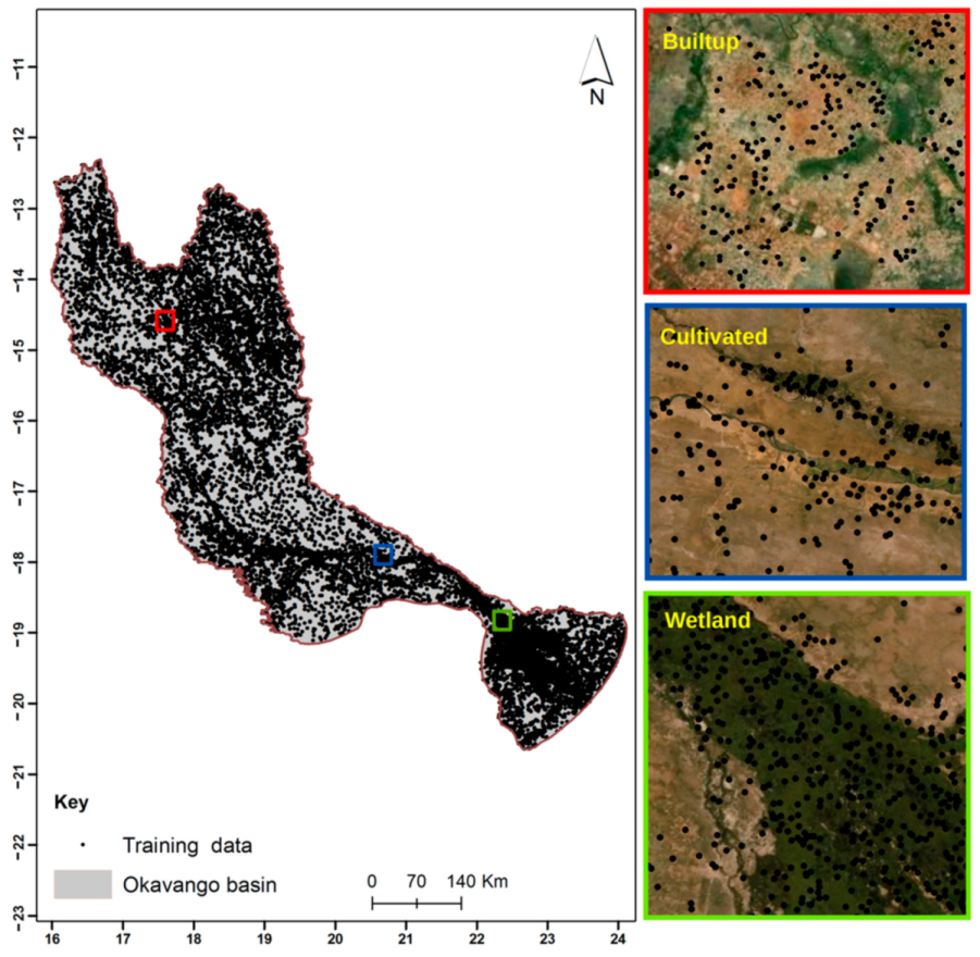
Before analysis, samples from different sources (ground samples and photo-interpreted samples) were merged in Quantum GIS 2.14 Essen (www.qgis.com, accessed on 20 March 2020). The spatial distribution of overall samples is depicted in Figure 2.

2.2.4. Experimental Design

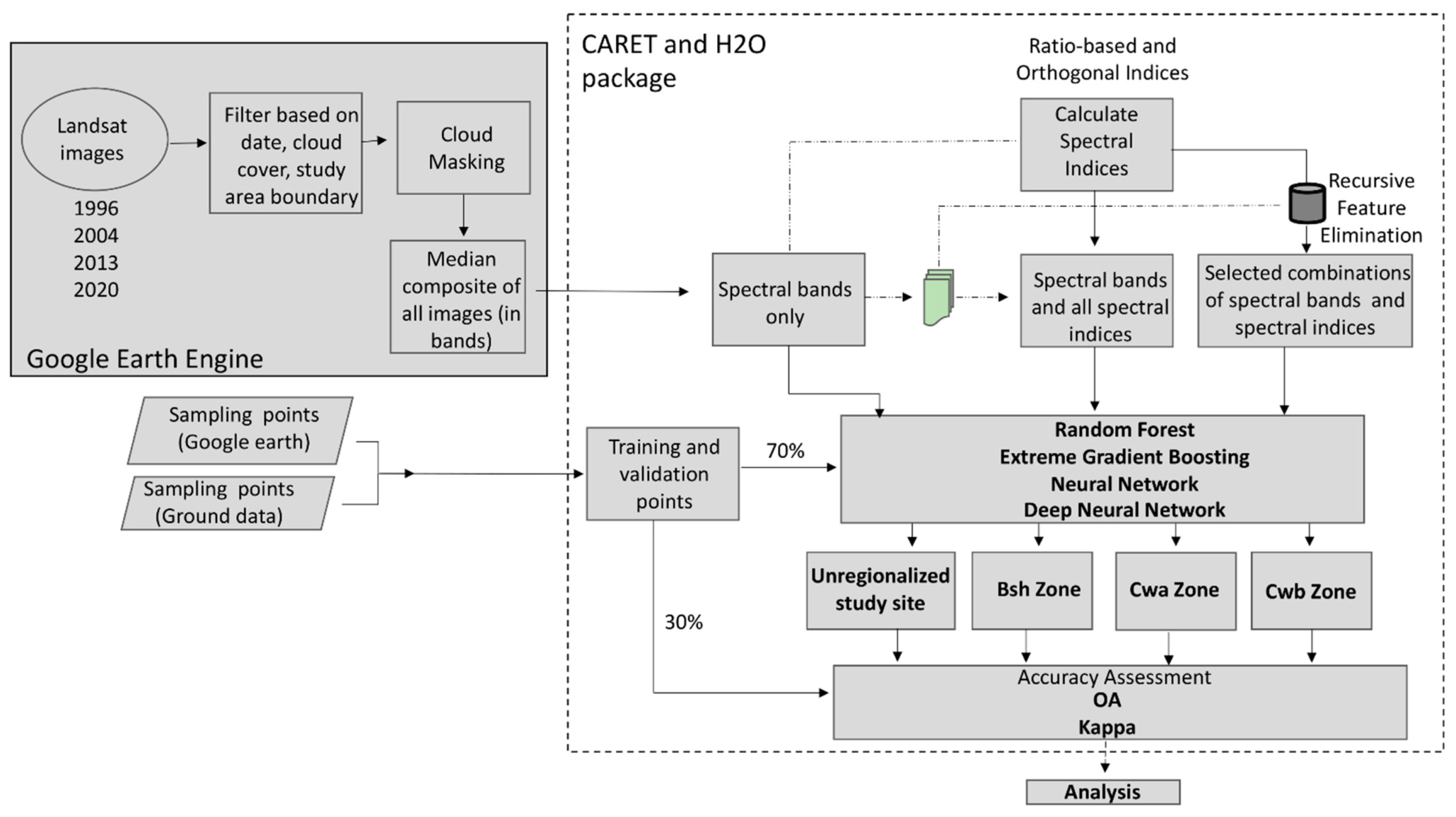
The study was designed to assess the value of integrating spectral bands with spectral indices and the significance of climate-based regionalization on the accuracy of LULC classification in a complex heterogeneous landscape. Two experiments were set. The first experiment investigated the value of the inclusion of spectral indices and feature selection, and the second assessed the value of climate-based regionalization on the accuracy of LULC classification in the Okavango Basin The study was conducted using R-statistics. The workflow of the study design is depicted in Figure 3.
The following sections give a detailed description of the methods.

2.2.5. Inclusion of Spectral Indices and Feature Selection

The analysis was run using combinations of seven spectral bands, eight RBS indices, and three OS indices. The first analysis was run using spectral bands only, the second using a combination of all spectral bands and spectral indices, and the third using a combination of spectral bands and spectral indices following a feature selection. Random forest-based recursive feature elimination (RF-RFE) was used for feature selection following recommendations by [33]. RF-RFE uses the provided input features and the random forest classifier to select the best combination of features based on feature importance [28,46]. To make the best combination of features, the RF-RFE iterates over various feature combinations through a repeated 10-cross validation and eliminates the least important features until the most parsimonious model is identified [75]. In this study, the RF-RFE is tuned to repeatedly iterate 30 times over 20 features (bands and spectral indices) based on the caret package in R statistical software.

2.2.6. Climate Based Study Area Regionalization

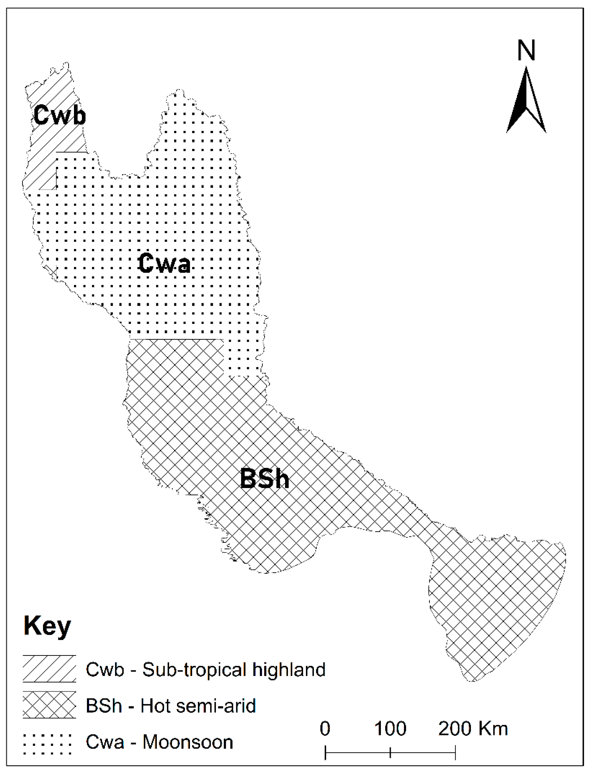
To evaluate the impact of climate-based regionalization on the accuracy of classification methods, the analysis was conducted first using the whole study area and thereafter based on the Koppen climate regions. Studies have reported that the performance of classifiers varies with space and time [76,77]. The Okavango Basin consists of the following climate zones, Cwa, Cwb, and Bsh Koppen zones (Figure 4).

2.2.7. LULC Classification Using Deep Learning and Machine Learning

Non-parametric DL and ML classifiers were used in this study. Two state-of-the-art ML classifiers, namely RF and XGBoost, were implemented using the caret package, and DL classifiers, namely neural network (Nnet) and DNN, were implemented using the caret and H20 packages in R statistics, respectively.

Machine Learning Classifiers

The RF classifier uses tree bagging to form an ensemble of trees by searching random subspaces in the given features and then splitting the nodes by minimizing the correlation between the trees [78]. The RF classifier has been widely used in landcover mapping [79,80,81]. Previous studies reported varying performance of the RF in different landscapes [82]. However, most studies claim that it is robust to overfitting and produces better accuracies with high efficiency when working with high dimensional data [78]. The major input parameters of the RF are the number of trees at each split (ntree) and the number of variables randomly sampled as candidates at each split (mtry).
The Xgboost algorithm is based on the boosting ensemble technique [76]. It builds on decision trees of weak learners that are combined into strong learners through an iterative process of learning from an ensemble of trees built on subsets of data. The models are weighted based on their performance and the ensemble model is built based on the weighted sum of the base layers [77]. Xgboost has been used in LULC mapping of numerous studies, in which it has outperformed the benchmark ML classifiers such as the RF and SVM [79,83]. The major parameters of the Xgboost include the maximum number of iterations (nround), maximum depth of a tree (max_depth), learning rate (eta), the minimum relative improvement in squared error reduction for a split to happen (gamma), and the minimum number of rows to assign to the terminal nodes (nodesize).

Deep Learning Classifiers

DL classifiers are based on neural networks [80]. They are biologically inspired algorithms that make predictions using a concept similar to an animal brain and its interconnections [84,85]. The basic structure of a neural network is a network of input layers that are connected to the output layer through hidden layers. This network of layers is responsible for transforming input data to output data with the help of activations and parameters. The weights on the nodes of each connection modify values at each neuron to determine how the input values are translated to output values. Neural networks require tuning, in which the tuning parameters and the number of layers involved make up the different types of DL models. In this study, the neural network (Nnet) algorithm and DNN are used.
The Nnet mimics a feed-forward neural network that uses the backpropagation algorithm for training coupled with one hidden layer [86]. To calibrate the Nnet algorithm, there are three important parameters required, namely the size, decay, and maxit, which control the number of neurons in the hidden layer, the weight decay, and the maximum number of iterations, respectively. Unlike the Nnet, the DNN uses a multi-layered feedforward neural network which comprises more than three hidden layers [44]. Ideally, increasing the number of hidden layers and neurons increases the potential to make predictions in complex situations [87]. The key parameters for DNN include the activation function (activation), number of hidden layers (hidden), size of each hidden layer (number of neurons per hidden layer), and the number of times to iterate (epoch). DL classifiers have shown good results in previous landcover studies [88,89].

Parameter Tuning of DL and ML Classifiers

In this study, parameter tuning (hyper parameterization) was performed to select the optimal parameters for each classifier. A repeated k-fold cross-validation technique was used based on a randomized sampling of hyperparameters reported in previous studies [90,91]. The optimization procedure was followed based on descriptions provided by Abdi [44]. The RF, Xgboost and Nnet were run using the caret package [75] and the DNN was run using the H2O package [85] in the R statistical software environment version 3.4.2 [92]. All computations were run on a Windows machine with 16 GB RAM and a Core i7 CPU@ 2.40 GHz made by Dell in China. Table 4 summarizes the optimal parameters that were determined for each classifier.

LULC Classification

For classification, sample points were randomly split 50 times into training (70%) and validation (30%) [93,94]. The classification was first run based on the whole study area and thereafter on each Koppen climate region. The classifications were separately run using three different combinations of bands and spectral indices as inputs per study site for the years 1996, 2004, 2013, and 2020. Average accuracy measures (overall accuracy and Kappa) were calculated from the model runs for each year. The results were then summarized for each classifier.

2.2.8. Accuracy Assessments and Validation

From each model run, 30% of the samples were randomly chosen from the overall sample set for validation. The validation samples were used to calculate overall accuracy (OA) and the Kappa statistic (Kappa) evaluations metrices. The OA ranges from 0 to 100, where 0 represents the lowest accuracy and 100 the highest, whereas Kappa ranges from 0 to 1, with 0 representing the lowest accuracy and 1 the highest accuracy [89]. Average OA and Kappa were calculated from model results of the four time-steps, namely 1996, 2004, 2013, and 2020. This was repeated for different combinations of spectral bands and indices under different study sites. The classification outputs were visually validated with high-resolution images (See Supplementary Figure S1). The proportions test (χ2 test) described by Agresti [90] was implemented in R software. The χ2 test was used to analyze the statistical difference in the performance of each classifier based on different combinations of spectral bands and spectral indices. A p < 0.05 was used as the critical level of significance.

3. Results

3.1. Integration of Spectral Indices to Spectral Bands

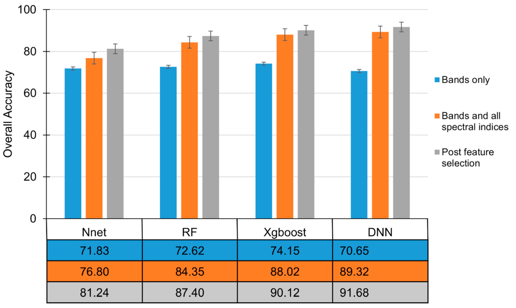
The results for the inclusion of spectral indices are given in Figure 5. Integrating spectral indices to bands increases the accuracy of LULC classification. Feature selection from combinations of bands and spectral indices further improves accuracy.
DNN recorded the highest OA, followed by Xgboost, RF, and Nnet (Figure 5). The average OA for inclusion of all spectral indices was 76.80, 84.35, 88.02, and 89.32 for Nnet, RF, Xgboost, and DNN, respectively. Regarding combinations of spectral bands and indices determined by feature selection (post-feature selection), the average OA was 81.24, 87.40, 90.12, and 91.68 for the Nnet, RF, Xgboost, and DNN, respectively. Improvement in accuracy based on post-feature selection combinations was significant for the DNN, RF, and Xgboost (p < 0.05); however, it was not significant for the Nnet. OA based on the post-feature selection combinations was not significantly different from that based on combinations of bands and all spectral indices (p > 0.05) for all the classifiers (see Supplementary Table S2).
Overall, the highest OA of 91.68 (Kappa = 0.90) was from the DNN based on the post-feature selection combination, which comprises an average of 13 features (See Supplementary Table S6). The lowest OA of 70.65 (Kappa = 0.68) was also for the DNN based on the bands only combination.
Overall, integration of bands and spectral indices appear to improve the accuracy of LULC classification in the unregionalized study site and the improvement further increases when implementing a feature selection. Although the integration with spectral indices and feature selection improves the accuracy, the improvement was not significant for all the classifiers. DL classifiers (DNN) generally yielded higher classification accuracies in comparison to ML classifiers (RF and Xgboost).

3.2. Climate Based Regionalization

3.2.1. Bsh-Hot Semi-Arid Zone

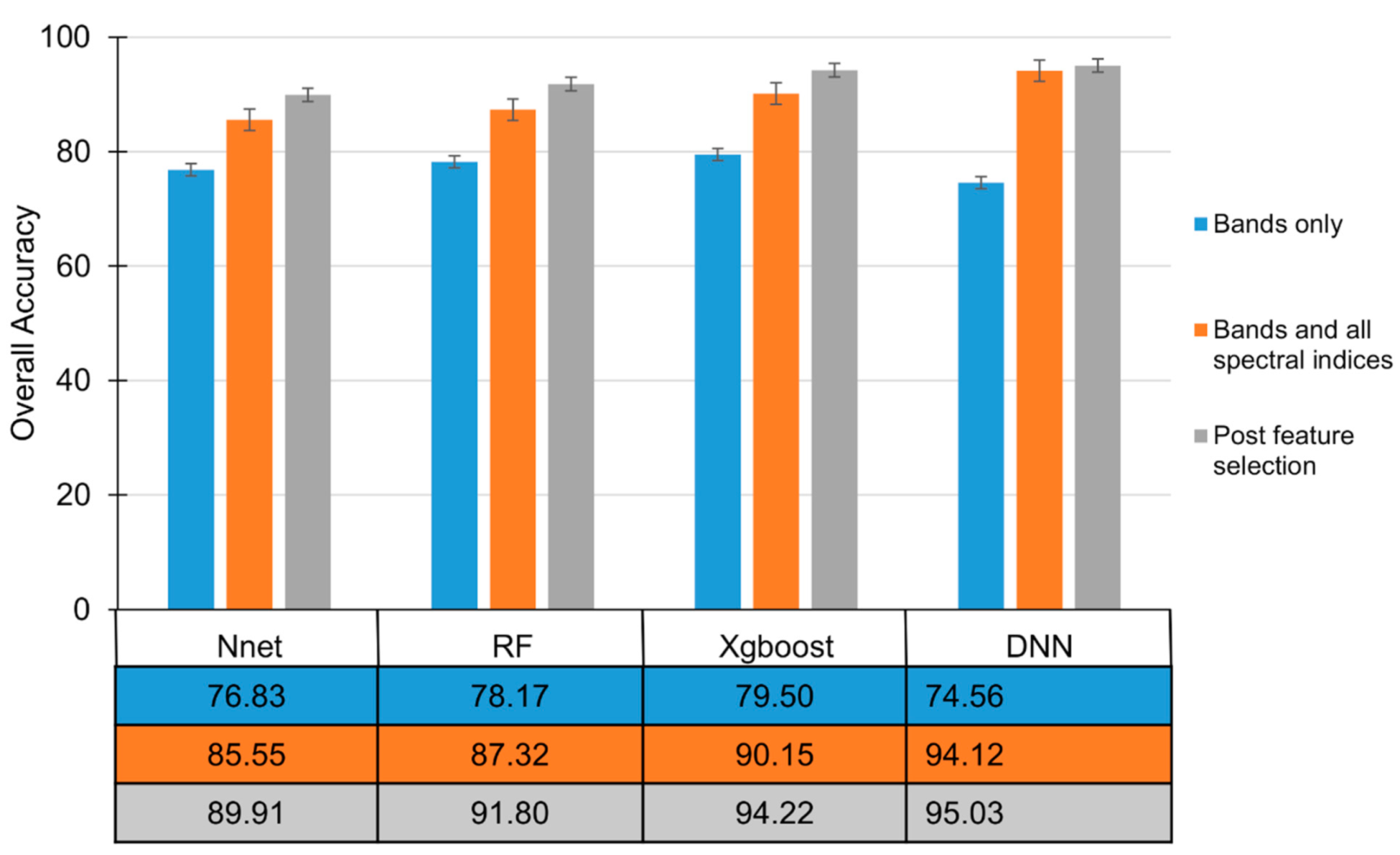
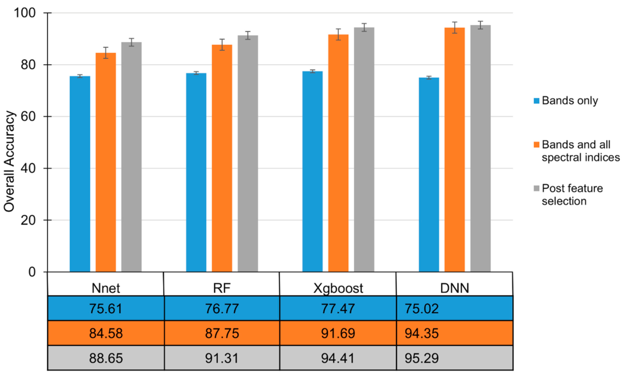
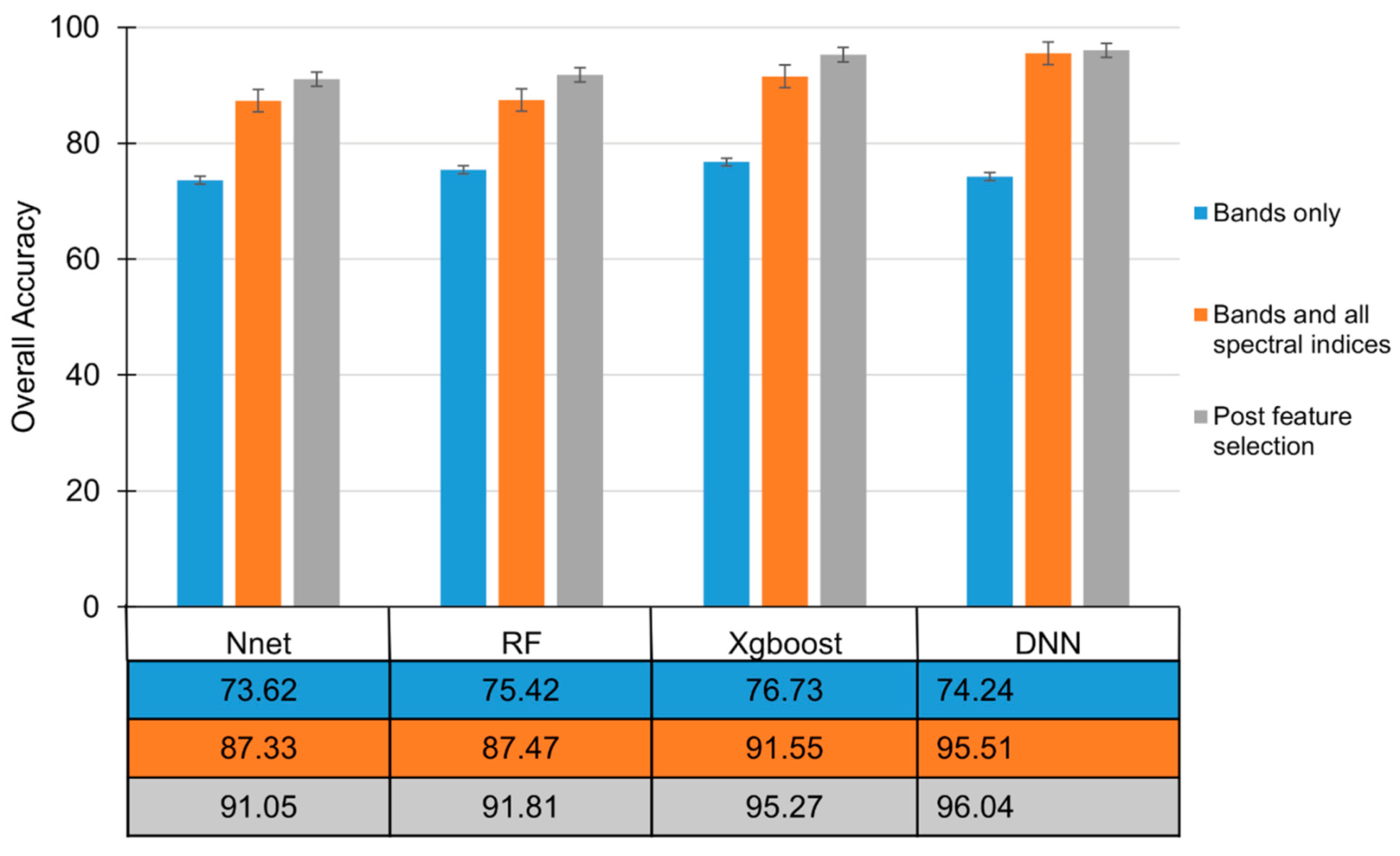
Results for climate-based regionalization based on Koppen–Geiger climate zones are depicted in Figure 6, Figure 7 and Figure 8.
For the Bsh hot semi-arid zone, the inclusion of spectral indices increased OA values to 85.55, 87.32, 90.15, and 94.12 for Nnet, RF, Xgboost and DNN, respectively (Figure 7). The kappa values were 0.84, 0.86, 0.88, and 0.92 for Nnet, RF, Xgboost, and DNN, respectively. DNN recorded the highest OA, followed by Xgboost, RF, and Nnet. Integration of bands with all spectral indices improved landcover classification significantly for the DNN classifier in the Bsh climate zone (p < 0.05). However, the OA did not improve significantly for the RF, Xgboost, and Nnet (p > 0.05). It can be seen that DL classifiers (DNN) benefited more from the inclusion of all spectral indices (improvement in OA > 20) compared to ML classifiers (Xgboost and RF); however, DL classifiers did not benefit as much from feature selection as ML classifiers did.
Concerning combinations of spectral bands and indices following a feature selection (post-feature selection) for the Bsh zone, OA values for Nnet, RF, Xgboost, and DNN increased from 76.83 to 89.91, 78.17 to 91.80, 79.50 to 94.22, and 74.56 to 95.03, respectively (Figure 8). DNN yielded the highest OA of 95.03 (Kappa = 0.93) using an average of 11 features (see Supplementary Table S7). Although post-feature selection combinations significantly improved accuracy for all the classifiers (p < 0.05), their OA is not significantly different from those using combinations of bands and all spectral indices (p > 0.05).

3.2.2. Cwa-Monsoon

As in the Bsh zone, the inclusion of spectral indices improved classification accuracy under the Cwa Koppen zone (Figure 7). Based on the inclusion of all spectral indices for the Cwa zone, OA accuracies increased from 75.61 to 84.58, 76.77 to 87.75, 77.47 to 91.69, and 75.02 to 94.35 for the Nnet, RF, Xgboost, and DNN, respectively. Integrating bands with spectral indices significantly improved the performance of the DNN and Xgboost (p > 0.05); however, it did not significantly improve the accuracy of Nnet and RF.
With regards to post-feature selection combinations for the Cwa zone, OA values increased to 88.65, 91.31, 94.41, and 95.29 for Nnet, RF, Xgboost, and DNN, respectively. The highest improvement was recorded based on the DNN from a combination of 10 features. In comparison to OA values from the bands only combination, the post-feature selection combinations yielded significantly higher accuracy for all classifiers (p < 0.05). However, OA values for post-feature selection combinations (based on 10 features) were not significantly different from OA values for combinations of bands and all spectral indices (p > 0.05). It can be seen that DL (DNN) classifiers did not benefit much from feature selection (improvement in OA < 2).

3.2.3. Cwb-Sub-Tropical Highland

As with the Bsh and Cwa zones, the inclusion of all spectral indices for the Cwb Koppen zone improved the accuracy (Figure 8). Integration of spectral indices with bands increased OA from 73.62 to 87.33, 75.42 to 87.47, 76.73 to 91.55, and 74.24 to 95.51 for Nnet, RF, Xgboost, and DNN, respectively. A similar pattern was observed when incorporating post-feature selection combinations, in which the DNN recorded the highest accuracy (OA = 96.04, Kappa = 0.95), followed by Xgboost (OA = 95.27, Kappa = 0.94), RF (OA = 91.81, Kappa = 0.90), and Nnet (OA = 91.05, Kappa = 0.89). Although improvements in accuracy following the inclusion of all spectral indices significantly improved the accuracy of most classifiers (Nnet, Xgboost, and DNN), the improvement was not significant for the RF classifier (p > 0.05). Unlike with the bands and all indices combination, incorporation of the post-feature selection combination (based on 15 features) significantly improved the accuracy of all the classifiers in the Cwb zone (p < 0.05). However, the OA values based on the post-feature selection combination were not significantly different from that of the bands and all indices combination for all the classifiers (p > 0.05).
In general, a combined inclusion of spectral indices and regionalization using climatic zones increase the accuracy of LULC classification using DL and ML classifiers. Climate-based regionalization and inclusion of spectral indices with bands did not statistically improve the accuracy of LULC consistently for all the ML and DL classifiers investigated in this study. However, climate-based regionalization and incorporation of post-feature selection combinations significantly improved the accuracy of LULC consistently for all the DL and ML classifiers used in this study. However, it was observed that the OA based on incorporating bands and all spectral indices was not significantly different from that based on the incorporation of post-feature selection combinations. This suggests that, although there are benefits of feature selection to accuracy when compared to mere incorporation of all features, the margin of benefit is slight. However, it appears that incorporating an average of about 15 features (based on feature selection) is sufficient to dramatically improve the accuracy of LULC more than what is achieved with a set of 20 features (bands and all indices). Overall, DNN consistently outperformed Xgboost, RF, and Nnet.

4. Discussion

Results show that climate-based regionalization and integration of spectral bands with indices improve the accuracy of LULC in the Okavango Basin. Additionally, incorporation of feature selection to combinations of bands and indices further enhances the accuracy. Statistical results show that the integration of indices and feature selection for unregionalized study areas does not significantly improve the performance of all the classifiers consistently. However, regionalization based on Koppen zones significantly improves LULC accuracy for all the classifiers. This is attributable to a reduction in spatiotemporal variability as a result of climate regionalization. This observation is in line with previous studies, which reported that spatiotemporal variability due to atmospheric conditions, soil moisture, sun elevation, view angle, and topography causes the similarity of spectral signatures of landcover types that are spectrally different [95,96].
Regionalization creates zones that have uniform ecological and spectral characteristics, thereby controlling the sensitivity of spectral signatures to LULC variation in heterogeneous landscapes and enhancing the efficiency of classifiers [12]. Noormets [97] and Richardson et al. [93], concurred that climate influences the phenology of vegetation cover and other ecosystem processes by driving the seasonality of albedo, surface roughness length, canopy conductance, and fluxes of water. Since optical remote sensing depends on reflectance, which is mainly influenced by phenology, regionalization based on climate systems could enhance the distinguishing of LULC classes [12,98]. While regionalization based on climate zones shows great potential in enhancing accuracy, intra-climate zone heterogeneity could potentially compromise LULC accuracy. In this study, spectral indices and feature selection in Koppen–Geiger regionalized study sites were integrated to further refine the LULC classification. The effects of including spectral indices to enhance accuracy when mapping LULC have been reported before. Mushore et al. [23] evaluated the inclusion of RBS indices when using the SVM on an urban landscape and found that the inclusion of indices yielded an increase in OA from 82.65 to 89.33. Results for the current study yielded higher accuracy values as compared to previous studies. OA values for the DNN based on bands and all spectral indices in this study improved from 74.24 to 96.04. This could be due to variation in the classifiers used, the number of training samples, and the scale at which the study was conducted. Mushore et al. [23] used 840 training samples on a study site with an extent of 94,000 ha. In this study, 5140 samples were used and the extent of the study area was 22,489,464 ha based on the Nnet, RF, Xgboost, and DNN classifiers. Notwithstanding that, their findings concurred with our findings that spectral indices improve the definition of LULC classes by enhancing the separability of one class against another. That said, Zeng et al. [99] assert that when spectral indices are used together with spectral bands in LULC classification, they have little effect on accuracy, as the addition of spectral indices only yielded a slight increase in OA, from 76.43 to 76.55. Their study only used RBS indices without incorporating feature selection on an unregionalized local study site using only the RF classifier. In this study, RF yielded higher accuracies, with OA ranging between 72.62 and 87.75. The strength of this study rests in that it incorporated regionalization, OS indices, and feature selection on a highly heterogeneous transboundary basin. Although previous studies have separately reported the effect of regionalization and incorporation of spectral indices in enhancing LULC maps [53,100], the combined effect of regionalization based on climate zones, the inclusion of spectral indices, and feature selection in a heterogeneous TDB is novel. This study is amongst the first to provide evidence for the combined influence of climate-based regionalization and integration of spectral bands with indices to enhance the accuracy of LULC maps in a TDB setting.
This research reveals that incorporation of feature selection improves accuracy more than the mere inclusion of all indices in all study sites and classifiers investigated. This finding agrees with previous studies, which reported that using feature selection has a crucial impact on the improvement of LULC accuracy [101,102]. Unlike simply including all features, feature selection helps to remove redundant features that tend to introduce the problems of dimensionality and uncertainty in model performance [103,104]. Feature selection creates parsimonious models that have high predictive power even with fewer variables. Although feature selection improves OA, in this study, OA of the post-feature selection combinations was not statistically significant from that of bands and all indices. This finding is in line with that of Georganos et al. [83], who observed that the increase in accuracy (OA from 77.7 to 78.9) based on feature selection (using the RFE) for the RF classifier was not significant. This is likely a result of RF having high predictive accuracy and effectively deducing patterns from data owing to its bagging and random algorithms [102,105,106]. Our findings for Xgboost are, however, contrary to those of Georganos et al. [83], who reported a significant increase in accuracy following the incorporation of post-feature selection combinations. This could be because of the variation in the number and type of features that they incorporated in their analysis as compared to those of the current study. Their study used a total of 169 features that include band descriptive statistics, gray level co-occurrence matrix (GLCM) for each spectral band, object compactness, perimeter, area, fractal dimension, and spectral indices as the initial input to the classification, whereas the current study only used 20 features of raw bands and spectral indices. A wide array of features could provide a large pool from which feature selection algorithms can draw, resulting in a larger improvement in accuracy. Although their study observed significant improvements in accuracy, their peak OA (79.8) was achieved using more features (23). The current study used fewer features (15), but achieved better peak OA (95.27).The strength of this study lies in the incorporation of combinations of RBS and OS indices together with climate-based regionalization, which aids in distinguishing land cover classes [21].
This study determined that DL classifiers (DNN) consistently yield more accurate results than ML classifiers (Xgboost, RF). Furthermore, DNN outperformed its fellow DL classifier (Nnet). This is likely as a result of the DNN having an effective way of deducing patterns from data owing to its structured neural networks, which allow the hierarchical flow of information from the input layers to output layers through hidden layers and activation functions. This structure, coupled with the backpropagation of errors, allows refinement of predictions before they are finally incorporated into the output [100]. Unlike the Nnet classifier, DNN has an increased number of hidden layers and activation functions that boosts model approximations through iterating various learning parameter values when making predictions [102]. Unlike ML classifiers (Xgboost, RF), the DNN requires intensive parameterization, which refines its performance [103]. The results of this study are in line with those of Li et al. [46], who reported DNN to be superior in LULC accuracy when compared to other ML classifiers (RF, SVM, and MLC). Abdi [44], however, reported that the DNN was outperformed by the Xgboost and RF when evaluating the LULC of the boreal landscape based on Sentinel 2 imagery. Abdi [44] tuned the DNN using the tanh activator, which easily saturates and slows the DNN when input values are large [104]. This study has strength in that it used the rectifier activation, which can hold incremental gradient descent because of its non-saturating function, thereby yielding higher accuracies even with complex data [105].
With regards to ML classifiers, results of this study show the superiority of Xgboost over the RF classifier. This is confirmed by previous literature, which reported that Xgboost outperformed the RF classifier [107,108]. According to Georganoes et al. [107], Xgboost performed 5% better than RF. Saini and Ghosh [108] reported that Xgboost outperformed RF by 1%. The current study observed that Xgboost performed better in OA by 4%. Although the level of difference in accuracy varies, most studies attribute the improved performance of Xgboost to its use of a large number of tuning parameters as compared to that of RF [108]. This is further enhanced by its use of an ensemble of trees, which incorporate weaker learners to make final predictions [76]. Despite the fact that the findings of this study are in line with previous work, the maximum accuracy values reported for Xgboost in this study are better than those of previous studies (OA = 95.27). The results of the present work demonstrate the superiority and strength of climate-based regionalization coupled with rigorous integration of bands and indices in complex landscapes.

5. Conclusions

This study aimed to evaluate the significance of the integration of spectral indices with bands and of climate-based regionalization for enhance the accuracy of LULC based on Landsat imagery using ML and DL. The specific objectives of this study were, firstly, to assess the value of integrating spectral bands with spectral indices on the accuracy of land cover classification using ML and DL classifiers, secondly, to investigate the value of climate-based regionalization to improve the accuracy of LULC classification within the Okavango Basin, and thirdly, to assess the performance of ML and DL classifiers for climate-based regionalization and inclusion of spectral indices. Inclusion of all indices and combinations of post-feature selection were separately used for each analysis to assess their performance in enhancing LULC mapping in a TDB. The DNN, Xgboost, Nnet, and RF classifiers were used for LULC classification. Combinations of bands and all indices and post-feature selection were then separately implemented for each climate zone to assess the value of climate-based regionalization on LULC classification. The results show that:
(1)
Inclusion of spectral indices improves the accuracy of LULC mapping for both ML and DL (with increase in OA > 5%);
(2)
Conducting a feature selection when evaluating LULC classification further improves accuracy as compared to mere inclusion of all spectral indices (with increase in OA > 10%); however, the increase was not consistently significant for all the classifiers;
(3)
Combined incorporation of post-feature selection combinations and climate-based regionalization significantly improves LULC accuracy based on all DL and ML classifiers (p < 0.05);
(4)
DL classifiers performed better than ML classifiers in all study sites and combinations of bands and spectral indices.
Based on findings from this study, it is concluded that spectral indices, feature selection, and climate-based regionalization result in statistically more reliable results. Those who wish to perform multitemporal analysis in heterogeneous landscapes using ML and DL classifiers should also consider combining climate-based regionalization, the inclusion of spectral indices, and feature selection based on RF-RFE. Additionally, preference should be given to DL classifiers when analyzing LULC in complex environments.
Although this study answered an important question on the integration of spectral indices and the influence of climate-based regionalization on the accuracy of LULC classification in a heterogeneous transboundary basin, there are some limitations associated with it. The study could not test the effect of climate-based regionalization on other climate zones outside of the Okavango Basin or the role of socioeconomic variables in delineating regions. Future research should test the effect of climate-based regionalization on other TDBs that have a different mix of climate zones using combinations, while at the same time incorporating socioeconomic factors for the delineation of regions. Pixel-based supervised classification based on the ML and DL classifiers was used in this study; further studies should investigate the use of object-based and unsupervised classification. The use of higher-resolution images and fusing data from different sensors is also advocated for future investigations.

Supplementary Materials

The following are available online at https://www.mdpi.com/article/10.3390/rs13245054/s1, Figure S1: Land use/cover classification outputs during the years 1996, 2004, 2013, and 2020 together with corresponding very-high-resolution satellite images for validation. Classification results are derived from the top performing results; Table S1: Details of sources and acquisition dates of satellite images used in this study; Table S2: p-values of proportional test (X2) results for pairwise comparison of the performance of different combinations of spectral bands with spectral indices and post-feature selection combinations based on the unregionalized study site; Table S3: p-values of proportional test (X2) results for pairwise comparison of the performance of different combinations of spectral bands with spectral indices and post-feature selection combinations based on the Bsh Koppen climate zone; Table S4: p-values of proportional test (X2) results for pairwise comparison of the performance of different combinations of spectral bands with spectral indices and post-feature selection combinations based on the Cwa Koppen climate zone; Table S5: p-values of proportional test (X2) results for pairwise comparison of the performance of different combinations of spectral bands with spectral indices and post-feature selection combinations based on the Cwb Koppen climate zone; Table S6: List of important features determined for the different study years using the random forest-based recursive feature elimination (RF-RFE) technique in an unregionalized study site; Table S7: List of important features determined for the different study years using the random forest-based recursive feature elimination (RF-RFE) technique in the Bsh Koppen climate zone; Table S8: List of important features determined for the different study years using the random forest-based recursive feature elimination (RF-RFE) technique in the Cwa Koppen climate zone; Table S9: List of important features determined for the different study years using the random forest-based recursive feature elimination (RF-RFE) technique in the Cwb Koppen climate zone.

Author Contributions

Conceptualization: B.K., Z.E.M. and L.L.; Methodology: B.K., Z.E.M. and L.L.; Writing—original draft: B.K., Z.E.M. and L.L.; Writing—review and editing: B.K., Z.E.M. and L.L. All authors have read and agreed to the published version of the manuscript.

Funding

The authors received funding from the USAID Resilient Waters Project for this research under prime contract number 72067418C00007.

Institutional Review Board Statement

Not applicable.

Informed Consent Statement

Not applicable.

Data Availability Statement

Training data which was used in this study are available upon request from the authors.

Acknowledgments

We thank USAID Resilient Waters for funding this project, implemented under prime contract number 72067418C00007. Our appreciation goes to the OKACOM and Okavango Wildland Trust for supplying us with some ground data which was used in this study. We express our gratitude to Sally Kuiper for editing the manuscript for English. We also thank the Stellenbosch University Language Centre for reviewing the language and flow of the manuscript.

Conflicts of Interest

The authors declare that there exists no competing financial interests or personal relationship that could appear to influence the work reported in this study.

Abbreviations

BshMonsoon
BTCAPTasseled Cap Brightness Index
CARTClassification and Regression Tree
CwaSubtropical Highland
CwbHot Semi-Arid
DEMDigital Elevation Model
DNNDeep Neural Network
DTsDecision Tree
ESEcosysytem Services
EVIEnhanced Vegetation Index
FAOFood and Agriculture Organization
GEEGoogle Earth Engine
GTCAPTasseled Cap Greeness Index
k-NNk-Nearest Neighbors
LCCSLandcover Classification System
LULCLand Use/Cover
MLMachine Learning
MNDWIModified Normalised Difference Water Index
NDBalNormalised Difference Bareness Index
NDBINormalised Difference Builtup Index
NDTINormalised Difference Tillage Index
NDVINormalised Difference Vegetation Index
NDWINormalised Difference Water Index
NGOWPNational Geographic Okavango and Wilderness Project
NnetNeural Network Algorithm
NTCAPTasseled Cap Noise Index
OKACOMOkavango River Basin Water Commission
OSOrthogonal Spectral Indices
RBSRatio-Based Spectral Indices
RFRandom Forest
SADCSouthern African Development Community
SAVISoil-Adjusted Vegetation Index
SVMSupport Vector Machine
TDBsTransboundary Drainage Basins
WTCAPTasseled Cap Wetness Index
XgboostExtreme Gradient Boosting

References

  1. Rai, P.K.; Chandel, R.S.; Mishra, V.N.; Singh, P. Hydrological inferences through morphometric analysis of lower Kosi river basin of India for water resource management based on remote sensing data. Appl. Water Sci. 2018, 8, 15. [Google Scholar] [CrossRef] [Green Version]
  2. Bhattarai, K.K.; Pant, L.P.; FitzGibbon, J. Contested governance of drinking water provisioning services in Nepal’s transboundary river basins. Ecosyst. Serv. 2020, 45, 101184. [Google Scholar] [CrossRef]
  3. Haefner, A. Negotiating for Water Resources: Bridging Transboundary River Basins; Taylor & Francis: Oxfordshire, UK, 2016. [Google Scholar]
  4. Just, R.E.; Netanyahu, S. International water resource conflicts: Experience and potential. In Conflict and Cooperation on Trans-Boundary Water Resources; Just, R.E., Netanyahu, S., Eds.; Springer: Boston, MA, USA, 1998; pp. 1–26. [Google Scholar] [CrossRef]
  5. Iyob, B. Resilience and Adaptability of Transboundary Rivers: The Principle of Equitable Distribution of Benefits and the Institutional Capacity of the Nile Basin; Oregon State University: Corvallis, OR, USA, 2010. [Google Scholar]
  6. Dessu, S.B.; Melesse, A.M.; Bhat, M.G.; McClain, M.E. Assessment of water resources availability and demand in the Mara River Basin. CATENA 2014, 115, 104–114. [Google Scholar] [CrossRef]
  7. Barraqué, B.; Mostert, E. Transboundary River Basin Management in Europe. Human Development Report Office (HDRO), United Nations Development Programme (UNDP), HDOCPA-2006-21. October 2006. Available online: https://ideas.repec.org/p/hdr/hdocpa/hdocpa-2006-21.html (accessed on 6 October 2020).
  8. Draper, S.E. Administration and institutional provisions of water sharing agreements. J. Water Resour. Plan. Manag. 2007, 133, 446–455. [Google Scholar] [CrossRef]
  9. Azgin, S.T.; Celik, F.D. Evaluating surface runoff responses to land use changes in a data scarce basin: A case study in Palas basin, Turkey. Water Resour. 2020, 47, 828–834. [Google Scholar] [CrossRef]
  10. Yang, Y.; Guan, H.; Batelaan, O.; McVicar, T.R.; Long, D.; Piao, S.; Liang, W.; Liu, B.; Jin, Z.; Simmons, C.T. Contrasting responses of water use efficiency to drought across global terrestrial ecosystems. Sci. Rep. 2016, 6, 23284. [Google Scholar] [CrossRef] [Green Version]
  11. Manandhar, R.; Odeh, I.O.; Ancev, T. Improving the accuracy of land use and land cover classification of Landsat data using post-classification enhancement. Remote Sens. 2009, 1, 330–344. [Google Scholar] [CrossRef] [Green Version]
  12. Kassawmar, T.; Eckert, S.; Hurni, K.; Zeleke, G.; Hurni, H. Reducing landscape heterogeneity for improved land use and land cover (LULC) classification across the large and complex Ethiopian highlands. Geocarto Int. 2018, 33, 53–69. [Google Scholar] [CrossRef] [Green Version]
  13. Dhanaraj, K.; Angadi, D.P. Land use land cover mapping and monitoring urban growth using remote sensing and GIS techniques in Mangaluru, India. GeoJournal 2020, 1–27. [Google Scholar] [CrossRef]
  14. Coskun, H.G.; Tanik, A.; Alganci, U.; Cigizoglu, H.K. Determination of environmental quality of a drinking water reservoir by remote sensing, GIS and regression analysis. Water Air Soil Pollut. 2008, 194, 275–285. [Google Scholar] [CrossRef]
  15. Johnson, B.A.; Iizuka, K. Integrating OpenStreetMap crowdsourced data and Landsat time-series imagery for rapid land use/land cover (LULC) mapping: Case study of the Laguna de Bay area of the Philippines. Appl. Geogr. 2016, 67, 140–149. [Google Scholar] [CrossRef]
  16. Mohajane, M.; Essahlaoui, A.; Oudija, F.; Hafyani, M.E.; Hmaidi, A.E.; Ouali, A.E.; Randazzo, G.; Teodoro, A.C. Land use/land cover (LULC) using Landsat data series (MSS, TM, ETM+ and OLI) in Azrou Forest, in the Central Middle Atlas of Morocco. Environments 2018, 5, 131. [Google Scholar] [CrossRef] [Green Version]
  17. Evrendilek, F.; Gulbeyaz, O. Boosted decision tree classifications of land cover over Turkey integrating MODIS, climate and topographic data. Int. J. Remote Sens. 2011, 32, 3461–3483. [Google Scholar] [CrossRef]
  18. Piyoosh, A.K.; Ghosh, S.K. Analysis of land use land cover change using a new and existing spectral indices and its impact on normalized land surface temperature. Geocarto Int. 2020, 1–23. [Google Scholar] [CrossRef]
  19. Tucker, C.J. Red and photographic infrared linear combinations for monitoring vegetation. Remote Sens. Environ. 1979, 8, 127–150. [Google Scholar] [CrossRef] [Green Version]
  20. Elvidge, C.D.; Lyon, R.J. Influence of rock-soil spectral variation on the assessment of green biomass. Remote Sens. Environ. 1985, 17, 265–279. [Google Scholar] [CrossRef]
  21. Lawrence, R.L.; Ripple, W.J. Comparisons among vegetation indices and bandwise regression in a highly disturbed, heterogeneous landscape: Mount St. Helens, Washington. Remote Sens. Environ. 1998, 64, 91–102. [Google Scholar] [CrossRef]
  22. Huete, A.R.; Jackson, R.D. Soil and atmosphere influences on the spectra of partial canopies. Remote Sens. Environ. 1988, 25, 89–105. [Google Scholar] [CrossRef]
  23. Mushore, T.D.; Mutanga, O.; Odindi, J.; Dube, T. Assessing the potential of integrated Landsat 8 thermal bands, with the traditional reflective bands and derived vegetation indices in classifying urban landscapes. Geocarto Int. 2017, 32, 886–899. [Google Scholar] [CrossRef]
  24. Guyon, I.; Elisseeff, A. An introduction to feature extraction. In Feature Extraction; Springer: Berlin/Heildelberg, Germany, 2006; pp. 1–25. [Google Scholar]
  25. Gilbertson, J.K.; Kemp, J.; van Niekerk, A. Effect of pan-sharpening multi-temporal Landsat 8 imagery for crop type differentiation using different classification techniques. Comput. Electron. Agric. 2017, 134, 151–159. [Google Scholar] [CrossRef] [Green Version]
  26. Rodriguez-Galiano, V.F.; Ghimire, B.; Rogan, J.; Chica-Olmo, M.; Rigol-Sanchez, J.P. An assessment of the effectiveness of a random forest classifier for land-cover classification. ISPRS J. Photogramm. Remote Sens. 2012, 67, 93–104. [Google Scholar] [CrossRef]
  27. Shahi, K.; Shafri, H.Z.M.; Hamedianfar, A. Road condition assessment by OBIA and feature selection techniques using very high-resolution WorldView-2 imagery. Geocarto Int. 2017, 32, 1389–1406. [Google Scholar] [CrossRef]
  28. Poona, N.K.; van Niekerk, A.; Nadel, R.L.; Ismail, R. Random forest (RF) wrappers for waveband selection and classification of hyperspectral data. Appl. Spectrosc. 2016, 70, 322–333. [Google Scholar] [CrossRef]
  29. Das, H.; Naik, B.; Behera, H.S. A Jaya algorithm based wrapper method for optimal feature selection in supervised classification. J. King Saud Univ. Comput. Inf. Sci. 2020. [Google Scholar] [CrossRef]
  30. Saeys, Y.; Inza, I.; Larranaga, P. A review of feature selection techniques in bioinformatics. Bioinformatics 2007, 23, 2507–2517. [Google Scholar] [CrossRef] [PubMed] [Green Version]
  31. Fourie, C. A One-Class Object-Based System for Sparse Geographic Feature Identification; University of Stellenbosch: Stellenbosch, South Africa, 2011. [Google Scholar]
  32. Elmannai, H.; Al-Garni, A.D. Classification using semantic feature and machine learning: Land-use case application. Telkomnika 2021, 19, 1242–1250. [Google Scholar] [CrossRef]
  33. Ismail, R.; Mutanga, O. Discriminating the early stages of Sirex noctilio infestation using classification tree ensembles and shortwave infrared bands. Int. J. Remote Sens. 2011, 32, 4249–4266. [Google Scholar] [CrossRef]
  34. Narumalani, S.; Zhou, Y.; Jelinski, D.E. Utilizing geometric attributes of spatial information to improve digital image classification. Remote Sens. Rev. 1998, 16, 233–253. [Google Scholar] [CrossRef]
  35. Homer, C.; Huang, C.; Yang, L.; Wylie, B.; Coan, M. Development of a 2001 national land-cover database for the United States. Photogramm. Eng. Remote Sens. 2004, 70, 829–840. [Google Scholar] [CrossRef] [Green Version]
  36. Manis, G.; Homer, C.; Ramsey, R.D.; Lowry, J.; Sajwaj, T.; Graves, S. The development of mapping zones to assist in land cover mapping over large geographic areas: A case study of the Southwest ReGAP Project. GAP Anal. Bull. 2000, 9, 13–16. [Google Scholar]
  37. Langrange, A.; Fauvel, M.; Grizonnet, M. Large-scale feature selection with Gaussian mixture models for the classification of high dimensional remote sensing images. IEEE Trans. Comput. Imaging 2017, 3, 230–242. [Google Scholar] [CrossRef] [Green Version]
  38. Tuia, D.; Persello, C.; Bruzzone, L. Domain adaptation for the classification of remote sensing data: An overview of recent advances. IEEE Geosci. Remote Sens. Mag. Int. J. Remote Sens. 2016, 4, 41–57. [Google Scholar]
  39. Beck, H.E.; Zimmermann, N.E.; McVicar, T.R.; Vergopolan, N.; Berg, A.; Wood, E.F. Present and future Köppen-Geiger climate classification maps at 1-km resolution. Sci. Data 2018, 5, 180214. [Google Scholar] [CrossRef] [PubMed] [Green Version]
  40. Weber, T. Okavango basin–Climate. Biodivers Ecol. 2013, 5, 15–17. [Google Scholar] [CrossRef] [Green Version]
  41. Aburas, M.M.; Ahamad, M.S.S.; Omar, N.Q. Spatio-temporal simulation and prediction of land-use change using conventional and machine learning models: A review. Environ. Monit. Assess. 2019, 191, 205. [Google Scholar] [CrossRef]
  42. Litjens, G.; Kooi, T.; Bejnordi, B.E.; Setio, A.A.A.; Ciompi, F.; Ghafoorian, M.; Van Der Laak, J.A.; Van Ginneken, B.; Sánchez, C.I. A survey on deep learning in medical image analysis. Med. Image Anal. 2017, 42, 60–88. [Google Scholar] [CrossRef] [Green Version]
  43. El Bouchefry, K.; de Souza, R.S. Learning in big data: Introduction to machine learning. In Knowledge Discovery in Big Data from Astronomy and Earth Observation; Elsevier: Amsterdam, The Netherlands, 2020; pp. 225–249. [Google Scholar]
  44. Abdi, A.M. Land cover and land use classification performance of machine learning algorithms in a boreal landscape using Sentinel-2 data. GIScience Remote Sens. 2020, 57, 1–20. [Google Scholar] [CrossRef] [Green Version]
  45. Li, W.; Fu, H.; Yu, L.; Gong, P.; Feng, D.; Li, C.; Clinton, N. Stacked autoencoder-based deep learning for remote-sensing image classification: A case study of African land-cover mapping. Int. J. Remote Sens. 2016, 37, 5632–5646. [Google Scholar] [CrossRef]
  46. Ligate, E.J.; Chen, C.; Wu, C. Evaluation of tropical coastal land cover and land use changes and their impacts on ecosystem service values. Ecosyst. Health Sustain. 2018, 4, 188–204. [Google Scholar] [CrossRef] [Green Version]
  47. Talukdar, N.R.; Ahmed, R.; Choudhury, P.; Barbhuiya, N.A. Assessment of forest health status using a forest fragmentation approach: A study in Patharia Hills Reserve Forest, northeast India. Model. Earth Syst. Environ. 2020, 6, 27–37. [Google Scholar] [CrossRef]
  48. Tsai, C.-F.; Hsiao, Y.-C. Combining multiple feature selection methods for stock prediction: Union, intersection, and multi-intersection approaches. Decis. Support. Syst. 2010, 50, 258–269. [Google Scholar] [CrossRef]
  49. Mendelsohn, J.; El Obeid, S. Okavango River: The Flow of a Lifeline; Struik Publishers: Cape Town, South Africa, 2004. [Google Scholar]
  50. Revermann, R.; Finckh, M.; Stellmes, M.; Strohbach, B.J.; Frantz, D.; Oldeland, J. Linking land surface phenology and vegetation-plot databases to model terrestrial plant α-diversity of the Okavango Basin. Remote Sens. 2016, 8, 370. [Google Scholar] [CrossRef] [Green Version]
  51. Mianabadi, A.; Davary, K.; Mianabadi, H.; Karimi, P. International environmental conflict management in transboundary river basins. Water Resour. Manag. 2020, 34, 3445–3464. [Google Scholar] [CrossRef]
  52. Porto, J.G.; Clover, J. The peace dividend in Angola: Strategic implications for Okavango basin cooperation. In Transboundary Rivers, Sovereignty and Development: Hydropolitical Drivers in the Okavango River Basin; African Water Issues Research Unit: Pretoria, South Africa, 2003. [Google Scholar]
  53. Steudel, T.; Göhmann, H.; Flügel, W.A.; Helmschrot, J. Assessment of hydrological dynamics in the upper Okavango river basins. Biodivers. Ecol. 2013, 5, 247–262. [Google Scholar] [CrossRef] [Green Version]
  54. Ge, Y.; Hu, S.; Ren, Z.; Jia, Y.; Wang, J.; Liu, M.; Zhang, D.; Zhao, W.; Luo, Y.; Fu, Y.; et al. Mapping annual land use changes in China’s poverty-stricken areas from 2013 to 2018. Remote Sens. Environ. 2019, 232, 111285. [Google Scholar] [CrossRef]
  55. Wingate, V.R.; Phinn, S.R.; Kuhn, N.; Bloemertz, L.; Dhanjal-Adams, K.L. Mapping decadal land cover changes in the woodlands of north eastern Namibia from 1975 to 2014 using the Landsat satellite archived data. Remote Sens. 2016, 8, 681. [Google Scholar] [CrossRef] [Green Version]
  56. Xiong, J.; Thenkabail, P.S.; Tilton, J.C.; Gumma, M.K.; Teluguntla, P.; Oliphant, A.; Congalton, R.G.; Yadav, K.; Gorelick, N. Nominal 30-m cropland extent map of continental Africa by integrating pixel-based and object-based algorithms using Sentinel-2 and Landsat-8 data on Google Earth Engine. Remote Sens. 2017, 9, 1065. [Google Scholar] [CrossRef] [Green Version]
  57. Avogo, W.; Agadjanian, V. Childbearing in crisis: War, migration and fertility in Angola. J. Biosoc. Sci. 2008, 40, 725. [Google Scholar] [CrossRef]
  58. Chaves, M.E.D.; Picoli, M.C.A.; Sanches, I.D. Recent applications of Landsat 8/OLI and Sentinel-2/MSI for land use and land cover mapping: A systematic review. Remote Sens. 2020, 12, 3062. [Google Scholar] [CrossRef]
  59. Zha, Y.; Gao, J.; Ni, S. Use of normalized difference built-up index in automatically mapping urban areas from TM imagery. Int. J. Remote Sens. 2003, 24, 583–594. [Google Scholar] [CrossRef]
  60. Chen, X.; Vierling, L.; Rowell, E.; DeFelice, T. Using lidar and effective LAI data to evaluate IKONOS and Landsat 7 ETM+ vegetation cover estimates in a ponderosa pine forest. Remote Sens. Environ. 2004, 91, 14–26. [Google Scholar] [CrossRef]
  61. Xu, H. Modification of normalised difference water index (NDWI) to enhance open water features in remotely sensed imagery. Int. J. Remote Sens. 2006, 27, 3025–3033. [Google Scholar] [CrossRef]
  62. Sturari, M.; Frontoni, E.; Pierdicca, R.; Mancini, A.; Malinverni, E.S.; Tassetti, A.N.; Zingaretti, P. Integrating elevation data and multispectral high-resolution images for an improved hybrid land use/land cover mapping. Eur. J. Remote Sens. 2017, 50, 1–17. [Google Scholar] [CrossRef]
  63. Farr, T.G.; Rosen, P.A.; Caro, E.; Crippen, R.; Duren, R.; Hensley, S.; Kobrick, M.; Paller, M.; Rodriguez, E.; Roth, L.; et al. The shuttle radar topography mission. Rev. Geophys. 2007, 45. [Google Scholar] [CrossRef] [Green Version]
  64. Rouse, J.W.; Haas, R.H.; Schell, J.A.; Deering, D.W. Monitoring vegetation systems in the greant plains with ERTS. In Proceedings of the Third Earth Resources Technology Satellite-1 Symposium, Washington, WA, USA, 10–14 December 1973; Nasa Special Publication; NASA: Washington, WA, USA, 1974; Volume 351, pp. 309–317. [Google Scholar]
  65. Van Deventer, A.P.; Ward, A.D.; Gowda, P.H.; Lyon, J.G. Using thematic mapper data to identify contrasting soil plains and tillage practices. Photogramm. Eng. Remote Sens. 1997, 63, 87–93. [Google Scholar]
  66. Zhao, H.; Chen, X. Use of normalized difference bareness index in quickly mapping bare areas from TM/ETM+. In Proceedings of the International Geoscience and remote Sensing Symposium, Seoul, Korea, 29 July 2005; Volume 3, p. 1666. [Google Scholar]
  67. Huete, A.; Didan, K.; Miura, T.; Rodriguez, E.P.; Gao, X.; Ferreira, L.G. Overview of the radiometric and biophysical performance of the MODIS vegetation indices. Remote Sens. Environ. 2002, 83, 195–213. [Google Scholar] [CrossRef]
  68. Huete, A.R. A soil-adjusted vegetation index (SAVI). Remote Sens. Environ. 1988, 25, 295–309. [Google Scholar] [CrossRef]
  69. Crist, E.P.; Cicone, R.C. A physically-based transformation of thematic mapper data—The TM tasseled cap. IEEE Trans. Geosci. Remote Sens. 1984, 3, 256–263. [Google Scholar] [CrossRef]
  70. Baig, M.H.A.; Zhang, L.; Shuai, T.; Tong, Q. Derivation of a tasselled cap transformation based on Landsat 8 at-satellite reflectance. Remote Sens. Lett. 2014, 5, 423–431. [Google Scholar] [CrossRef]
  71. De Sousa, C.; Fatoyinbo, L.; Neigh, C.; Boucka, F.; Angoue, V.; Larsen, T. Cloud-computing and machine learning in support of country-level land cover and ecosystem extent mapping in Liberia and Gabon. PLoS ONE 2020, 15, e0227438. [Google Scholar]
  72. Arino, O.; Ramos, J.; Kalogirou, V.; Defourny, P.; Achard, F. GlobCover 2009. In Proceedings of the ESA Living Planet Symposium, Bergen, Norway, 27 June–2 July 2010. [Google Scholar]
  73. Foody, G.M.; Mathur, A. Toward intelligent training of supervised image classifications: Directing training data acquisition for SVM classification. Remote Sens. Environ. 2004, 93, 107–117. [Google Scholar] [CrossRef]
  74. Di Gregorio, A. Land Cover Classification System: Classification Concepts and User Manual: LCCS; Food & Agriculture Org.: Rome, Italy, 2005; Volume 2. [Google Scholar]
  75. Kuhn, M. Caret: Classification and Regression Training; Astrophysics Source Code Library: Houghton, MI, USA, 2015; p. ascl-1505. [Google Scholar]
  76. Chen, T.; Guestrin, C. Xgboost: A scalable tree boosting system. In Proceedings of the 22nd ACM SIGKDD International Conference on Knowledge Discovery and Data Mining, San Francisco, CA, USA, 13–17 August 2016; pp. 785–794. [Google Scholar]
  77. Rousset, G.; Despinoy, M.; Schindler, K.; Mangeas, M. Assessment of deep learning techniques for land use land cover classification in southern New Caledonia. Remote Sens. 2021, 13, 2257. [Google Scholar] [CrossRef]
  78. Breiman, L.; Friedman, J.; Stone, C.J.; Olshen, R.A. Classification and Regression Trees; CRC Press: Boca Raton, FL, USA, 1984. [Google Scholar]
  79. Saini, R.; Ghosh, S.K. Ensemble classifiers in remote sensing: A review. In Proceedings of the 2017 International Conference on Computing, Communication and Automation (ICCCA), Greater Noida, India, 5–6 May 2017; pp. 1148–1152. [Google Scholar]
  80. Schmidhuber, J. Deep learning in neural networks: An overview. Neural Netw. 2015, 61, 85–117. [Google Scholar] [CrossRef] [Green Version]
  81. Atkinson, P.M.; Tatnall, A.R. Introduction neural networks in remote sensing. Int. J. Remote Sens. 1997, 18, 699–709. [Google Scholar] [CrossRef]
  82. Talukdar, S.; Singha, P.; Mahato, S.; Pal, S.; Liou, Y.-A.; Rahman, A. Land-use land-cover classification by machine learning classifiers for satellite observations—A review. Remote Sens. 2020, 12, 1135. [Google Scholar] [CrossRef] [Green Version]
  83. Georganos, S.; Grippa, T.; Vanhuysse, S.; Lennert, M.; Shimoni, M.; Wolff, E. Optimizing classification performance in an object-based very-high-resolution land use-land cover urban application. In Remote Sensing Technologies and Applications in Urban Environments II; SPIE: Bellingham, WA, USA, 2017; Volume 10431, p. 104310I. [Google Scholar]
  84. Kuhn, M.; Johnson, K. Applied Predictive Modeling; Springer: Berlin/Heildelberg, Germany, 2013; Volume 26. [Google Scholar]
  85. Cook, D. Practical Machine Learning with H2O: Powerful, Scalable Techniques for Deep Learning and AI; O’Reilly Media, Inc.: Newton, MA, USA, 2016. [Google Scholar]
  86. Werbos, P.J. Supervised learning: Can it escape its local minimum? In Theoretical Advances in Neural Computation and Learning; Springer: Berlin/Heildelberg, Germany, 1994; pp. 449–461. [Google Scholar]
  87. Singh, C.; Murdoch, W.J.; Yu, B. Hierarchical interpretations for neural network predictions. arXiv 2018, arXiv:180605337. [Google Scholar]
  88. Omer, G.; Mutanga, O.; Abdel-Rahman, E.M.; Adam, E. Exploring the utility of the additional WorldView-2 bands and support vector machines in mapping land use/land cover in a fragmented ecosystem, South Africa. S. Afr. J. Geomat. 2015, 4, 414–433. [Google Scholar] [CrossRef] [Green Version]
  89. Congalton, R.G. A review of assessing the accuracy of classifications of remotely sensed data. Remote Sens. Environ. 1991, 37, 35–46. [Google Scholar] [CrossRef]
  90. Agresti, A. Categorical Data Analysis; John Wiley & Sons: Hoboken, NJ, USA, 2003; Volume 482. [Google Scholar]
  91. Mongus, D.; Žalik, B. Segmentation schema for enhancing land cover identification: A case study using Sentinel 2 data. Int. J. Appl. Earth Obs. Geoinf. 2018, 66, 56–68. [Google Scholar] [CrossRef]
  92. R Development Core Team. R Foundation for statistical Computing; R Development Core Team: Vienna, Austria, 2014. [Google Scholar]
  93. Richardson, A.D.; Keenan, T.F.; Migliavacca, M.; Ryu, Y.; Sonnentag, O.; Toomey, M. Climate change, phenology, and phenological control of vegetation feedbacks to the climate system. Agric. For. Meteorol. 2013, 169, 156–173. [Google Scholar] [CrossRef]
  94. Reed, B.C.; Schwartz, M.D.; Xiao, X. Remote sensing phenology. In Phenology of Ecosystem Processes; Springer: Berlin/Heildelberg, Germany, 2009; pp. 231–246. [Google Scholar]
  95. Abdullah, A.Y.M.; Masrur, A.; Adnan, M.S.G.; Baky, M.; Al, A.; Hassan, Q.K.; Dewan, A. Spatio-temporal patterns of land use/land cover change in the heterogeneous coastal region of Bangladesh between 1990 and 2017. Remote Sens. 2019, 11, 790. [Google Scholar] [CrossRef] [Green Version]
  96. Löw, F.; Michel, U.; Dech, S.; Conrad, C. Impact of feature selection on the accuracy and spatial uncertainty of per-field crop classification using support vector machines. ISPRS J. Photogramm. Remote Sens. 2013, 85, 102–119. [Google Scholar] [CrossRef]
  97. Noormets, A. Phenology of Ecosystem Processes: Applications in Global Change Research; Springer: Berlin/Heildelberg, Germany, 2009. [Google Scholar]
  98. Belgiu, M.; Drăguţ, L. Random forest in remote sensing: A review of applications and future directions. ISPRS J. Photogramm. Remote Sens. 2016, 114, 24–31. [Google Scholar] [CrossRef]
  99. Zeng, H.; Wu, B.; Wang, S.; Musakwa, W.; Tian, F.; Mashimbye, Z.E.; Poona, N.; Syndey, M. A synthesizing land-cover classification method based on Google Earth engine: A case study in Nzhelele and Levhuvu Catchments, South Africa. Chin. Geogr. Sci. 2020, 30, 397–409. [Google Scholar] [CrossRef]
  100. Candel, A.; Parmar, V.; LeDell, E.; Arora, A. Deep learning with H2O; H2O Ai Inc.: Mountain View, CA, USA, 2016; pp. 1–21. [Google Scholar]
  101. Ma, L.; Li, M.; Ma, X.; Cheng, L.; Du, P.; Liu, Y. A review of supervised object-based land-cover image classification. ISPRS J. Photogramm. Remote Sens. 2017, 130, 277–293. [Google Scholar] [CrossRef]
  102. Beysolow, T., II. Introduction to Deep Learning Using R: A Step-by-Step Guide to Learning and Implementing Deep Learning Models Using R; Apress: New York, NY, USA, 2017. [Google Scholar]
  103. Goodfellow, I.; Bengio, Y.; Courville, A. Deep Learning; MIT Press: Cambridge, MA, USA, 2016. [Google Scholar]
  104. Shi, W.; Gong, Y.; Ding, C.; Tao, Z.M.; Zheng, N. Transductive semi-supervised deep learning using min-max features. In Proceedings of the European Conference on Computer Vision (ECCV), Munich, Germany, 8–14 September 2018; pp. 299–315. [Google Scholar]
  105. Nair, V.; Hinton, G.E. Rectified Linear Units Improve Restricted Boltzmann Machines; University of Toronto: Toronto, ON, Canada, 2010. [Google Scholar]
  106. Mustapha, I.B.; Saeed, F. Bioactive molecule prediction using extreme gradient boosting. Molecules 2016, 21, 983. [Google Scholar] [CrossRef] [Green Version]
  107. Georganos, S.; Grippa, T.; Vanhuysse, S.; Lennert, M.; Shimoni, M.; Wolff, E. Very high resolution object-based land use–land cover urban classification using extreme gradient boosting. IEEE Geosci. Remote Sens. Lett. 2018, 15, 607–611. [Google Scholar] [CrossRef] [Green Version]
  108. Saini, R.; Ghosh, S.K. Analyzing the impact of red-edge band on land use land cover classification using multispectral RapidEye imagery and machine learning techniques. J. Appl. Remote Sens. 2019, 13, 044511. [Google Scholar] [CrossRef]
Figure 1. Study area map showing the location of the Okavango Basin in relation to countries that belong to the Southern African Development Community (SADC) region.
Remotesensing 13 05054 g001
Figure 2. Map showing training and validation points that were used in this study. The zoom-outs show training points overlaid on high-resolution imagery.
Remotesensing 13 05054 g002
Figure 3. Study workflow.
Remotesensing 13 05054 g003
Figure 4. Map showing the Koppen–Geiger climate regions in the Okavango Basin.
Remotesensing 13 05054 g004
Figure 5. Comparison of the performance of the neural network (Nnet), random forest (RF), extreme gradient boosting (Xgboost), and deep neural network (DNN) classifiers for the integration of spectral bands with different spectral indices and post-feature selection combinations based on an unregionalized study site.
Remotesensing 13 05054 g005
Figure 6. Comparison of the performance of the neural network (Nnet), random Forest (RF), extreme gradient boosting (Xgboost), and deep neural network (DNN) classifiers for the integration of spectral bands with different spectral indices and post-feature selection combinations based on the Bsh Koppen zone.
Remotesensing 13 05054 g006
Figure 7. Comparison of the performance of the neural network (Nnet), random forest (RF), extreme gradient boosting (Xgboost), and deep neural network (DNN) classifiers for the integration of spectral bands with different spectral indices and post-feature selection combinations based on the Cwa Koppen zone.
Remotesensing 13 05054 g007
Figure 8. Comparison of the performance of the neural network (Nnet), random forest (RF), extreme gradient boosting (Xgboost), and deep neural network (DNN) classifiers for the integration of spectral bands with different spectral indices and post-feature selection combinations based on the Cwb Koppen zone.
Remotesensing 13 05054 g008
Table 1. Ratio based spectral indices used in this study.
Name of Spectral IndicesFormulaeReferences
NDVI N I R R E D N I R + R E D [64]
NDBI S W I R 1 N I R S W I R 1 + N I R [59]
NDWI G R E E N N I R G R E E N + N I R [60]
MNDWI G R E E N S W I R 1 G R E E N + S W I R 1 [61]
NDTI S W I R 1 S W I R 2 S W I R 1 + S W I R 2 [65]
NDBal S W I R 1 T I R S 1 S W I R 1 + T I R S 1 [66]
EVI 2.5 ( N I R R E D N I R + 6 × R E D 7.5 × R E D + 1 ) [67]
SAVI 1.5 ( N I R R E D N I R + R E D ) [68]
Table 2. Orthogonal spectral indices used in this study.
Landsat 5
Name of Spectral IndicesTransformation CoefficientsReferences
(Blue)
Band 1
(Green)
Band 2
(Red)
Band 3
(NIR)
Band 4
(SWIR1)
Band 5
(SWIR2)
Band 7


[69]
BTCAP0.20430.41580.55240.57410.31240.2303
GTCAP−0.16030.2819−0.49340.79400.00020.1446
WTCAP0.03150.20210.31020.15940.68060.6109
NTCAP−0.8242−0.08490.4392−0.05800.2012−0.2768
Landsat 8
Name of Spectral IndicesTransformation CoefficientsReferences
(Blue)
Band 2
(Green)
Band 3
(Red)
Band 4
(NIR)
Band 5
(SWIR1)
Band 6
(SWIR2)
Band 7


[70]
BTCAP0.30290.27860.47330.55990.50800.1872
GTCAP0.29410.24300.54240.72760.07130.1608
WTCAP0.15110.19730.32830.3407−0.71170.4559
NTCAP−0.8239−0.08490.4396−0.0580.2013−0.2773
Table 3. A summary of the number of training and validation samples that were used in this study.
Number of Sample Points
LULC ClassGround SamplesPhoto-Interpreted SamplesClass Total
bareland420242662
builtup612116728
water524156680
cultivated513114627
woodland63163694
shrubland212482694
grassland194321515
wetland314226540
Overall Total342017205140
Table 4. A summary of optimal parameters for ML and DL classifiers as determined from hyper-parameterization.
ModelParametersHyper-Parameter Values
RFmtry100
ntree2
Xgboostnrounds500
maxdepth7
eta0.01
gamma0.1
nodesize2
NnetSize70
learning rate0.005
maxit500
DNNactivationRectifier
hidden layers5
neurons per layer200
epochs300
Publisher’s Note: MDPI stays neutral with regard to jurisdictional claims in published maps and institutional affiliations.