Abstract
The Rohingya refugee influx to Bangladesh in 2017 was a historical incident; the number of refugees was so massive that significant impacts to local communities was inevitable. The Bangladesh government provided land in a preserved area for constructing makeshift camps for the refugees. Previous studies have revealed the land cover changes and impacts of the refugee influx around campsites, especially with regard to local forest resources. Our aim is to establish a convenient approach of providing up-to-date information to monitor holistic local situations. We employed a classic unsupervised technique—a combination of k-means clustering and maximum likelihood estimation—with the latest rich time-series satellite images of Sentinal-1 and Sentinal-2. A combination of VV and normalized difference water index (NDWI) images was successful in identifying built-up/disturbed areas, and a combination of VH and NDWI images was successful in differentiating wetland/saltpan, agriculture /open field, degraded forest/bush, and forest areas. By doing this, we provided annual land cover classification maps for the entire Teknaf peninsula for the pre- and post-influx periods with both fair quality and without prior training data. Our analyses revealed that on-going impacts were still observed by May 2021. As a simple estimation of the intervention consequence, the built-up/disturbed areas increased 6825 ha (compared with the 2015–17 period). However, while the impacts on the original forest were not found to be significant, the degraded forest/bush areas were largely degraded by 4606 ha. These cultivated lands would be used for agricultural activities. This is in line with the reported farmers’ increased income, despite local people with other occupations that are all equally facing the decreases in income. The convenience of our unsupervised classification approach would help keep accumulating a time-series land cover classification, which is important in monitoring impacts on local communities.
1. Introduction
In August 2017, the massive Rohingya refugee influx to Cox’s Bazar, Bangladesh from Rakhine state, Myanmar shocked the world. The Bangladesh government provided the land for constructing makeshift camps for the estimated 671,500 refugees at that time [1]. Because of the sheer number of refugees pouring in, as well as the country itself already having a highly dense population, the government needed to clear the preserved forest area in Cox’s Bazar. So far, several studies were conducted in order to evaluate the impacts on the local forest resources. Hassan et al. (2018) [2] estimated that 2283 ha of forestland were either lost or degraded, due to the campsite’s construction and expansion by December 2017. Hassan et al. (2020) [3] estimated that 1600 to 2200 ha of forestland was initially cleared, and 3200 ha of forest were either gone or degraded between 2017 and 2019. Hassan et al. (2018) [2], as well as Barun et al. (2019) [4], report the campsite specific estimation. Their findings reveal that the Kutupalong–Balukhali campsite showed the greatest camp expansion, which reached a net increase of 1219 ha by December 2017 and 1313 ha by February 2018, respectively. Barun et al. (2019) [4] reported that the camp areas further expanded, resulting in an area loss of 1800 ha of forest by March 2019.
In recent years, land cover classification has faced a turning point owing to the availability of high-quality remote sensing archives, as well as the advancements seen in machine learning technologies. Random forest and support vector machine have gained popularity as land cover classification approaches. These techniques are categorized as supervised classifications, which require training data as an information input. This assumes that an analyst has complete knowledge on local land cover classes; therefore, if any class is missed in the input information, the class will not be identified and will be treated as if it did not exist. In any cases, acquiring sufficient training samples is always challenging [4,5]. Unsupervised classification techniques use only the information in remote sensing images and do not require other prior information to obtain classification results. Because remote sensing images are susceptible to noise, classification results from unsupervised classifications are often inferior to supervised classification results. On the contrary, however, the non-requirement of a prior training input data is advantageous for when analysts want to know land cover changes that are caused by unordinary external disturbances, such as disasters, climate change, and human intervention.
When land cover classification includes vegetation covers, the strong impact of phenology is underlined; therefore, the use of limited number images has potentially caused a phenological bias that can lead to false land cover classification [4]. Dense time series data can efficiently capture the phenological stages that sometimes change extensively within a short period, as well as contributing to a better quality of vegetation classification [6]. The Land Remote Sensing Satellite (Landsat) images, as well as the recently available Sentinel-2 (S2) images, have both been commonly used in land cover classification due to their high availability [7]. However, because these are optical images, which are influenced by atmospheric conditions, good quality images can be limited in certain areas during certain seasons; for instance, tropical regions during monsoon season. In such conditions, the areas are often covered by clouds and the ground surface reflectance cannot be acquired by satellite sensors. The Sentinel-1 (S1) satellite is equipped with a synthetic aperture radar (SAR), which is primarily independent from cloud cover; therefore, it can acquire imagery—regardless of the weather—over the whole year and at regular intervals. Recently, many attempts of using both SAR images and optical images for crop classification have been widely undertaken [3,4,8,9] and has recognized the S1 SAR data as a promising alternative to optical remote sensing data for both land cover and crop classification in cloudy and rainy areas [10].
In this article, we annually analyze the land cover changes around the Rohingya refugee campsites in Cox’s Bazar District in Bangladesh from 2015 to 2021. We employ an unsupervised classification technique in contrast to the aforementioned studies related to the Rohingya refugee case, most of which employed supervised machine learning classification approaches with a small number of images. We demonstrate that the larger number of input images can compensate for prior training data by using all available free S1 and S2 images throughout the study period (about 45 images for each year). The classification technique employed in this study is a classic unsupervised method: a combination of the k-means clustering and maximum likelihood estimation. We attempt to establish a systematic way to find the most suitable parameter settings for the unsupervised classification. By doing so, we verify how the advanced development of both the sensors and internet environment improved the usability of the technique. We applied our approach to elucidate how the study area that is adjacent to the refugee camps has been exposed to the ever-changing interventions due to the massive influx of Rohingya refugees; a historical incident of which the impact it has had on local communities is yet to be fully realized. The aim of this study is to monitor these impacts in a convenient, transparent, and reproducible way.
2. Materials and Methods
2.1. Study Area
The Rohingya refugee campsites are located in two upazilas, Ukhia and Teknaf, of the Cox’s Bazar district in Chittagong division, Bangladesh, which is situated in the Teknaf peninsula. An upazila is an administrative unit that is under the district’s administration. After August 25, 2017—with the massive influx of refugees pouring in—they were placed in a total of 34 camps. The average population density was estimated at nearly 40,000 people per km2, with a total of 855,000 Rohingya refugees in December 2019 [11]. According to the 2010 national census, the local population was 207,379 and 264,389 in the Ukhia and Teknaf upazilas, respectively [12]. The Rohingya populations outnumbered the local population. Figure 1 shows the camp site locations; they are situated inside of and adjacent to the preserved areas Inani National Park (INP) and Teknaf Wild Sanctuary (TWS).
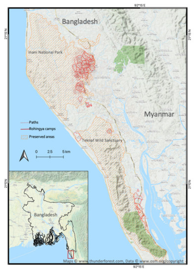
Figure 1.
Map of the study area. The map information of the campsites, Inani National Park, and Teknaf Wild Sanctuary (TWS) were obtained from [13], [3], and [14], respectively.
2.2. Remote Sensing Images
Satellite images were collected for both the pre-influx and post-influx period. Figure 2 shows the dataset overviews. Right after the Sentinel-1 and Sentinel-2 missions started the operation in 2014 and 2015, respectively, the number of downloadable images were limited. Therefore, we grouped the images available for the period when the first product was available in this area until 25 August 2017; we then used them as an input dataset for the pre-influx period. Regarding the images for the post-influx period, our aim was for a yearly classification, so about one year after 25 August 2017 was excluded from the analysis; this is because the campsite construction was on-going and the land cover was assumed unstable. Thus, we collected the images while also considering the local major irrigation practice for Aman rice cultivation (from 1 June 2018, until 31 May 2021); the images were grouped annually.
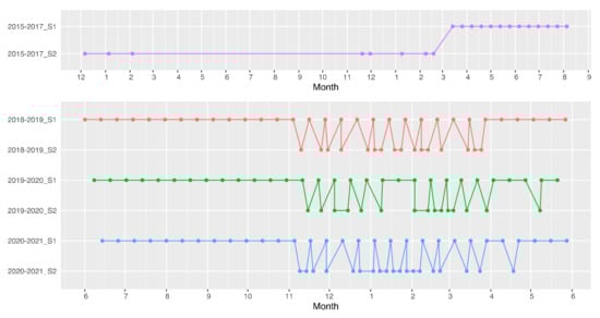
Figure 2.
Data acquisition dates chart. For the data visualization, the R [15] and the R package “ggplot2” [16] were used.
2.2.1. Sentinel-1 Dataset
Sentinel-1 (S1) products (10 m resolution) were acquired from the Alaska Satellite Facility (ASF). All the available Level-1 interferometric wide (IW) swath mode, ground range detected (GRD), high resolution (HR) products in dual polarization (VH and VV) in the study area (Path 41 and Frame 65) during the study period were downloaded from the Sentinel-1A and Sentinel-1B archives. The images were processed with the S1 toolbox in the Sentinel Application Platform (SNAP) and applied the ordinary steps: orbit correction, radiometric calibration, geometric correction, and conversion to decibel units. The detailed process is described elsewhere, such as in the work of Chakhar et al. (2021) [9]. The only difference here is the omission of the Speckle filtering application in our study. Speckle is random “salt-and-pepper” noise that deteriorates the image quality. Speckle filtering intends to mitigate the effect; however, it reduces image resolution appreciably and, as a result, the obtained image is blurred. Because the land covers are spatially fragmented in the study area, this could affect the visibility of the land cover classification results. Furthermore, Inglada et al. (2019) [17] reported that when both SAR and optical data are used together, Speckle filtering introduces a small improvement towards the end of the season. Van Ticht et al. (2018) [18] also suggested that by considering 12-day backscatter mosaics, as well as using time series as input features instead of single-date images, the impact of radar speckle could be minimized. We intended a yearly analysis, and not a data point (date)-wise analysis, so that as many images could be included; therefore, the random noise should be effectively mitigated. Thus, we decided not to apply Speckle filtering.
2.2.2. Sentinel-2 Dataset
Sentinel-2 (S2) products were acquired from the European Space Agency (ESA) Copernicus Open Access Hub. All the available images of less than 1% of cloud coverage in the study area covered by the Sentile-2 tile “46QDJ” during the study period were downloaded from both Sentinel-2A and Sentinel-2B archives. The obtained Level-1C products were atmospherically corrected using the Sen2cor algorithm and were then converted to the bottom-of-atmosphere (BOA) reflectance images and projected with Universal Transverse Mercator (UTM) Zone 46N. Both the normalized difference vegetation index (NDVI) and normalized difference water index (NDWI) were calculated. NDWI is calculated with Band 8 and Band 11. The Band 11 images, of which resolution are 20 m, were resampled to 10 m resolution by the nearest neighbor resampling method. The above procedures were conducted by the R [15] and the R package “Sen2r” [19]. The prepared images were visibly checked; furthermore, images that had no cloud cover were adopted for the successive land cover classification analysis. The final datasets are shown in Table 1.

Table 1.
The number of the images used for land cover classification.
2.3. Classification Procedures
2.3.1. Classification Technique
The VV and VH images from the S1 stack, as well as the NDVI and NDWI images from the S2 stack, were used in land cover classification. The ratio of VH/VV was often found to be significantly contributing to better crop classification results [6]. However, in our study, the target objects are not only limited to vegetation; in addition, the hilly steep areas are included, so that the backscatter coefficients can range from the negative values to the positive values. In such a case, the divided values sometimes take extreme numbers due to the very small denominators; this may potentially cause over-evaluation. Thus, we decided not to include the VH/VV ratio index in our analysis.
The Geographic Resources Analysis Support System (GRASS) platform in the QGIS 3.16.9 [20] was used in order to conduct the land cover classification. QGIS is an open-source geographic information system (GIS) application. Prior to the classification, all images (projected in UTM Zone 46N and WGS 1984 Datum) were clipped to the extent of Cox’s Bazar–Teknaf peninsula within the Bangladesh boundary. In the QGIS, the classification process was conducted by a successive operation with two functions. First, “i.cluster” was applied, which was considered a modified k-means clustering algorithm [21]; second, the maximum likelihood estimation was applied by “i.maxlik,” with the exported signature file from the “i.cluster” application. In the “i.cluster” algorithm, the sampling interval was set to 63 pixels for column and 31 pixels for row; the minimum pixel in a class was set to 17; the calculation convergence was judged if the assigned classes were stable for 98% of sample pixels (the above settings are the default of the software); the initial class number was set to 50; the maximum iteration was set to 500; and the minimum class separation distances (hereafter, called the class separation parameter) were set from 0.5 to 2.0, by 0.1 increases. The optimal class separation parameter is an image-specific number and requires experimentation. Commonly used minimum class separations range from 0.5 to 1.5 [22].
K-means clustering results are sensitive to the differences in variances of variables; therefore, we standardized each pixel value of an image by the mean and standard deviation calculated with the entire pixel values of the image. In doing this, the image would then have a mean of 0 and a variance of 1. Next, we also considered the differences in the numbers of images for each image type (such as VV and NDVI) by incorporating weights on variances. For example, when we use the 30 VV images and the 19 NDVI images, we multiplied the standardized pixel values of the NDVI images with 30/19 to make the contribution of each type of image to classification equal. The image preparation was conducted by the R [15] and the R package “raster” [23] and “rgdal” [24].
2.3.2. Classification Steps
The major challenge was being able to distinguish the campsites from paddy fields, which somehow tended to be classified as the same class. Therefore, the first step was dedicated to identifying the campsites. After trials with several combinations of the images, we succeeded in separating the campsites from paddy fields into the class “Built-up/Disturbed area” by using the VV images and NDWI images together. These were occupied with artificial objects, such as settlements, agricultural tents, and brickfields. Furthermore, they were exposed to unusual disturbance by artificial or natural events, such as construction, logging, and landslides. In the second step, we classified the remaining areas except for the built-up/disturbed areas by using the VH and NDWI images. We also tried several combinations of images (including NDVI); we came to the conclusion that the combination of the VH and NDWI images could most accurately separate wetland and paddy fields, as well as succeeding in consistently identifying the forest areas that have been preserved (according to our knowledge). The influences of the input imagery on the classification results will be discussed further in the discussion section.
2.3.3. Accuracy Assessment
The above two-step classification results were combined: the built-up/disturbed area is from the step 1 classification result, and other land covers are from the step 2 classification result. An accuracy assessment was conducted using the AcATaMa Plugin [25] within QGIS, which is based on the sampling design proposed by Olofsson et al. (2014) [26]. A stratified random sampling was applied, so that the number of samples were distributed according to the spatial share of each class in the combined classification image. A standard error was set to 0.01, which provided about 100 assessment points in each year group classification result. The Google Earth images for the corresponding years were used as the ground truth information; the images acquired on 1/27/2016, 11/23/2018, 1/20/2020, and 2/1/2021 were primarily referred for the year groups 2015–17, 2018–19, 2019–20, and 2020–21, respectively. In addition, the accuracy was also checked by comparing the previous studies conducted in the area.
3. Results
3.1. Parameter Selection
Figure 3 and Figure 4 show the relations between the class separation parameter values and corresponding resulted class numbers. Figure 3 shows the first step results for identifying the built-up/disturbed area with the VV and NDWI images; Figure 4 shows the second step results for classifying the land covers, except for the built-up/disturbed area with the VH and NDWI images. “Class separation” on the x-axis means the parameter value set for the class separation in “i.cluster” algorithm, and “Class numbers” on the left y-axis shows the resulting class numbers from the corresponding parameter value setting. “Rejection threshold” on the right y-axis represents the average of indexed results of a chi-square test conducted in “i.maxlik.” A total of 16 confidence intervals are predefined to determine the confidence level for each classified cell in the classified image, where the indexes are interpreted as 1 = keep and 16 = reject [27].
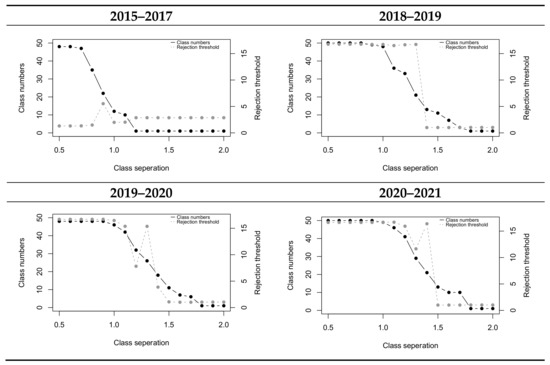
Figure 3.
Relations between class separation values and classification results from the VV and NDWI datasets (first step).
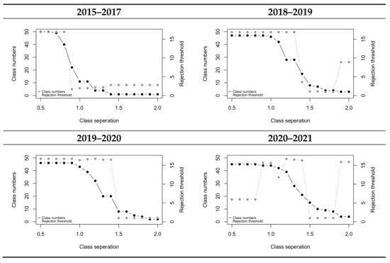
Figure 4.
Relations between class separation values and classification results from the VH and NDWI datasets (second step).
We adopted the class separation parameters at which the classification results started to be stable—namely at the knee of a curve according to the Elbow method—with regard to both the class number and rejection threshold value. This criterion provides the maximum class numbers among the acceptable results. Then, we interpreted the results and merged some of the classes if we identified them as the same land cover. The adopted parameters and resulting class numbers are shown in Table 2.
Table 2.
The adopted parameters and resulting class numbers.
3.2. Yearly Land Covers
Figure 5 shows the resulting land cover classification maps for each year group.
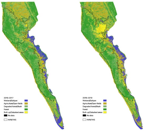
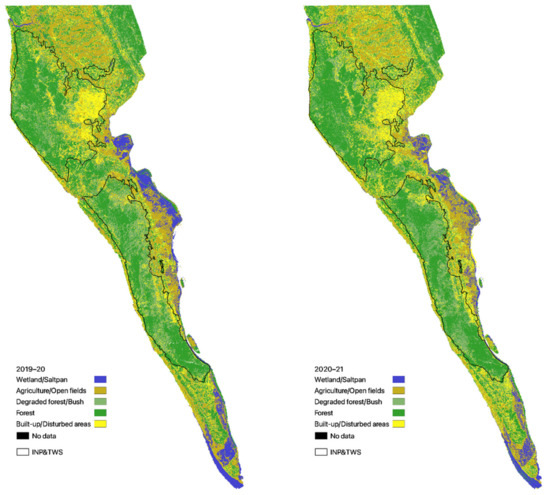
Figure 5.
Land cover classification results for each year group.
In order to make the land cover classification maps with the above parameter settings, the classes were interpreted according to the Google Earth images, our experiences in the study area, and consultation with a local collaborator. We merged the classes that were considered the same land cover. With that, we finally ended up with five classes; namely Wetland/Saltpan, Agriculture /Open fields, Degraded forest/Bush, Forest, and Built-up/Disturbed areas.
The class “Wetland/Saltpan” is significant in the eastern and southern directions of the study area. This area is famous for salt production, wherein the saltpans are distributed. The production is repeatedly conducted from November to May, which is almost the same period when the S2 images are available in the area. During this period, the saltpan is on and off with the sea water; thus, these areas were classified as the same class as the wetland in our analysis. Figure 6 shows the appearance of the saltpans.
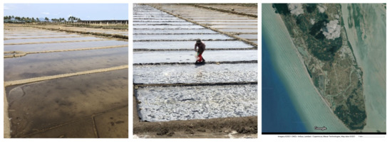
Figure 6.
Salt production. The left and center photos were taken by our local collaborator, Delwar Hossain. The Google Earth image shows the south part of the study area, the tip of the Teknaf peninsula.
The wetland was found at the hill ridges and sinks. This is due to the topographical complexity at these places, and the S1 images are sensitive to it. The wetland cannot be located in steep places, in principle; therefore, we reclassified the misclassified pixels as “No data.” We identified the “No data” class by the ratio of “Degraded forest/Bush” and “Forest” that surround the wetland pixels. In the area, the wetland is usually adjacent to agriculture/open fields; so when the ratio is high, such pixels were identified as non-wetland and subsequently reclassified as “No data.” Table 3 summarizes the class meanings.
Table 3.
Land cover classes and their definitions.
The accuracy was assessed with the Google Earth images from each year group; the results are shown in Table 4. The accuracy for 2015–17 was lower than those for other year groups. This is probably due to the 2015–17 classification using multiple year images. Furthermore, the accuracy judgement may not be consistent with what the classification result represented; this is because the classification was implemented for year(s) datasets, whereas the accuracy was assessed with one single day Google Earth image for each year group.
Table 4.
Accuracy assessment results.
To complement the accuracy assessment, we compared the present results with the previous literature. In the literature, the area information for the area size was, often times, not provided or the classes were not compatible to ours; therefore, the referenceable studies were limited. Figure 7 shows a comparison of the classification results in the Kutupalong–Balukhali expansion area with Braun et al. (2019) [4]. The result showed a similar tendency, although the “Open” class had a different meaning in the two studies. In our analysis, we have two kinds of open field classes: one is the same class as agriculture, and the other is recognized as disturbed areas. The open fields classified as disturbed areas have not been stable through the year and are exposed to any kind of significant disturbances. Therefore, for example, paths in the hills were classified as “Agriculture/Open fields” in the present analysis, and not as “Built-up/Disturbed areas,” because the paths tend to be stable. This classification characteristics are owed to the yearly set of S1 image attributes. As another reference, we compared the results with Hasan et al. (2020) [3]. They provided minute classifications. Considering their classes of homestead vegetation, mixed forest, plantation forest, canopy forest, and casurina as our class of “Forest;” as well as shrubs and degraded forest as our class of “Degraded Forest/Bush;” the estimated area size was 19,309.29 ha for forest and 10,664.24 ha for degraded forest/bush in 2017; and 17,465.95 ha for forest and 11,098.36 ha for degraded forest/bush in 2019. Our results were 17,657 ha for forest and 14,307 ha for degraded forest/bush in 2015–17; and 17,620 ha for forest and 11,080 ha for degraded forest/bush in 2018–19. The estimations for 2018–19 were quite close, and the difference in the 2017 classification might be caused from the differences in the considered years; we used a longer duration, rather than a single year for the 2015–17 classification due to the limitation of the available images.
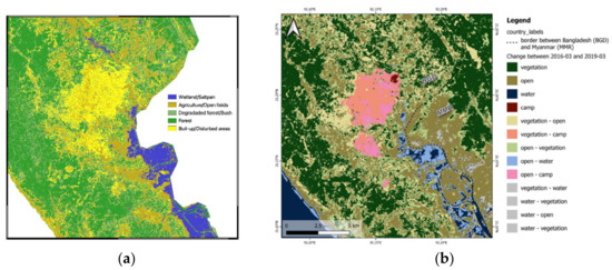
Figure 7.
A comparison of the identified campsite areas with the previous literature. (a) Results for the 2018–19 year group. (b) Adopted from Braun et al. (2019) (2016.03–2019.03) [4].
3.3. Land Cover Changes
Table 5 shows the land cover area for each class and each year group. The built-up/disturbed area significantly increased since the Rohingya refugee influx. The area 1 km from the camps was still being developed; however, the forest degradation has not been promoted in recent years according to the forest area changes in total area, INP, and TWS, 1 km from camps. In the TWS area, the forest has not been exposed to significant degradation.
Table 5.
Land cover area (in both ha and percentages) for each year group. The total area was the whole Teknaf peninsula, below the latitude 21°18′48.312″.
Table 6 shows the initial (2015 to 2017) classes of the built-up/disturbed areas in each year group. The row summation corresponds to the built-up/disturbed areas appeared in “Total” that were seen in Table 5. The deforestation, due to the intervention expansion, reached 1569 ha in 2020–21; furthermore, together with the degraded forest/bush clearance, it reached 6510 ha.
Table 6.
Changes from 2015–17 classes to built-up/disturbed areas (in ha) in each year group.
According to Table 5, the total forest area was 415 ha smaller in 2020–21 than in 2015–17; however, 1569 ha of forest was changed to the built-up/disturbed areas in 2020–21, as shown in Table 6. Therefore, 1154 ha of forest was regained in the non-built-up/disturbed areas. Table 7 shows the cross tabular between the 2015–17 and 2020–21 classes. The most significant contribution to afforestation is a shift from the degraded forest/bush to forest; however, the change from forest to degraded forest/bush was also salient. As a whole, the change from the degraded forest/bush to forest exceeded 999 ha, which mostly explained the 1154 ha difference.
Table 7.
Cross tabular of 2015–17 and 2020–21 classes (in ha).
Figure 8 shows the annual land cover changes associated with forest and the changes between 2015–17 and 2020–21. The land cover change from 2015–17 to 2018–19 (top left of Figure 8) reveals that the crucial impact on forest (pink pixels) occurred due to campsite construction. This impact was not significantly expanded afterward. In the same period, the forest degradation (red pixels) was salient in TWS; however, the afforestation (purple pixels) is observed in the subsequent years. Likewise, significant forest degradation can be observed in INP between 2018–19 and 2019–20 (top right of Figure 8); however, this loss was recovered in the next period. Overall, in the north-to-center area, the deforestation and the afforestation tended to appear as a cluster; whereas in the center-to-south area, these pixels are seen to be rather scattered.
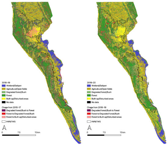
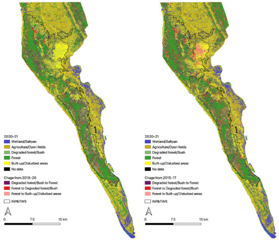
Figure 8.
Geographical distribution of forest-associated changes to land cover.
4. Discussion
4.1. Peculiarity of the Classification Approach
We found the result with VV and NDWI produced a more reasonable classification than other combinations with VH, VV, NDVI, and NDWI. The increase of the included image types, such as VH + VV + NDWI, did not outperform the present combination. Our assumption is that when each image type has independent information to each other, the result provides the most reasonable result; however, when each image type contains similar information, the information may be redundant and land cover classifications, therefore, do not perform well. Chakhar et al. (2020) [9] reported that the combination of S1 (VV + VH) + S2 (NDVI) performed the best in crop classifications by random forest; although the performances were only slightly different when VH and VV were combined with NDVI individually, and the combinations of VV + NDVI and VH + NDVI provided the tie F1 score. Veloso et al. (2017) [6] found the correlation between VH and NDVI for summer crops; however, VV and NDVI had associations for winter crops. Filgueiras et al. [28] stated that VV and VH were highly correlated with a higher range of NDVI larger than 0.25, which would eliminate the pixels where the soil reflectance is dominant. Singha et al. (2016) [29] and Nguyễn et al. (2016) [30] reported that the VH was more sensitive than the VV to capture rice growth stages when only the S1 images were used for classification. As was suggested by the previous studies, VV, VH, and NDVI are likely to contain similar information; according to our assumption, if we use any combination of these images for our unsupervised classification approach, the information will both be redundant and not able to provide a satisfactory result. Because of this, it did not work well in our case according to our assumption.
We had a relatively-good number of S2 images (10 to 15 images), and—in order to fully utilize the S1 and S2 image sets—we considered the NDWI to be included for an analysis. This was because the previous studies reported that the short wavelength infra-red (SWIR) band contained important information for crop classification [31,32]; in addition, one of the challenges we faced was classifying the paddy fields and wetland into different classes. The NDWI uses the SWIR band for calculation and is useful for identifying water contents. Then, we succeeded in separating the built-up/disturbed area in the first step with the VV + NDWI images and in the second step to separate wetland and paddy fields, as well as forest and degraded forest/bush areas with the VH + NDWI images. This approach worked, likely owing to the S1 backscatter characteristics. The VV backscatter is dominated by direct contributions from the ground and canopies, while the ground backscatter at the S1 C-band is affected by soil moisture, surface roughness, and terrain topography [33]; therefore, it was effective to identify the built-up/disturbed areas. The VH backscatter is dominated by the volume scattering mechanisms at the canopy of lower or sparse vegetation types [6,34]; this is so that it was effective at identifying paddy fields and degraded forest/bush areas. However, which combination of images is the best may be dependent on the area characteristics and target land covers.
Our unsupervised classification approach is useful when rich training data is not readily available due to limited physical and/or legitimate access to local fields and when the aim is to discover general land cover classifications. Trobik et al. [35] studied rice production practices in Myanmar with Landsat-8 OLI, PALSAR-2, and time series S1 data throughout 2015. They conducted this study from the perspective of food security by employing the satellite images because little data was available due to political factors. They first classified land cover for the entire country into the five classes—crop, water, forest, shrub, developed, like ours—with 1367 ground truth points obtained through field visits and 459 created polygons corresponding through random forest classification. Then, they extrapolated several indicators for monitoring rice cultivation with the time series S1 information of the classified crop areas. This is one of the cases where our unsupervised approach would be most effectively utilized. Moreover, land cover maps that are updated year by year could be produced by our method in a consistent manner.
Our unsupervised method requires prior information to confirm class meanings and to check our judgement with merging classes. Therefore, prior local knowledge is less crucial than with ordinary supervised methods which dictate the classification outcome based on the information from arbitrarily selected training areas. We have merged the resulted classes into five land cover categorizations, which is sufficient for our purpose. However, if we had different goals, we may have merged the resultant classes into the larger number of classes. In such a case, a single-date satellite image may not be sufficient in determining the class meanings, and thus, richer local information might be required. Still, the required information is less than what is needed for supervised classification because what is asked here is simply about the particularity of the land use in the focused class area compared with other classes areas. Therefore, one single question to a local expert is sufficient.
4.2. Impacts on Local Landscape
The result demonstrated that the built-up/disturbed areas are still being expanded after the campsite construction was completed a couple years ago. The largest impact was found in the degraded forest/bush class, whereas forest was once degraded but has since been regained. Figure 8 shows that the deforestation and afforestation are more likely to appear dispersed but coexist in close proximity to each other. This probably implies that local people circulate the locations of acquiring forest resources, and that some areas are either not intervened for preservation or simply because access to them is physically difficult. On the other hand, the deforested areas (the red pixels in Figure 8) that are adjacent to the built-up/disturbed areas will be unlikely to regain, which is often observed in INP; these areas would be converted to built-up/disturbed areas sooner or later. Built-up/disturbed areas are expanded around the built-up/disturbed areas and agriculture/open fields; this expansion was realized by clearing the degraded forest/bush areas. The expansion of built-up/disturbed areas was most probably for agriculture field development, owed mostly to the cheap labor that was supplied by Rohingya refuges. This assumption is in line with the finding by Ullah et al. (2021) [36]; the income was increased only for farmers and not for other occupations, such as business workers, fishermen, and laborers among local community dwellers, even though the significant wage depression after the influx was observed [37]. It is evident that the wage decreased due to the abundant labor supply by the Rohingya refugees; however, the demand for the agriculture increased because the land for cultivation expanded. Agriculture/open fields expansion was also found in the saltpan areas located in the east coast of the peninsula. This could be because either the water balance changed [37] or the cultivation practice changed. Local information and further investigation are both needed to determine the reason. Overall, our assessment elucidated that the impacts of the Rohingya refugees’ influx on the forest in the preserved areas were—so far—minimum. However, the pre-existing degraded forest/bush areas were largely lost, totaling 4606 ha in the entire study area and 1698 ha loss was found in INP. Most of this area was originally supposed to be forest, but due to the failure of the preservation activities in the past [38], the area has been degraded forest/bush. If these areas will be used for the agriculture, it will help increase the agricultural production and income of both the local people and the Rohingya refugees. It is undoubtedly a challenge to balance these consequences for the government, as well as the practitioners working in the area.
5. Conclusions
The Rohingya refugee influx to Bangladesh in 2017 was a historical incident, and the number of refugees was so massive that it was inevitable that local communities would be exposed to the significant impacts of this event. In principle, the refugees are not allowed to go outside of the camps legitimately and are also physically surrounded by barbed-wire fences. If the refugees stayed inside of the camps, as they were regulated, the interactions with the local landscape would have been minimum. However, this has not seemed to be the case thus far [39], and our time-series land cover classification analyses revealed that the impacts are still ongoing. As a simple estimation of the intervention consequence, the built-up/disturbed areas increased 6825 ha in the entire Teknaf peninsula by May 2021, compared to the 2015–17 period. We applied the unsupervised classification technique with a rich set of S1 and S2 images in order to investigate the impacts on the local landscape. The accuracy assessment, as well as a comparison with the previous studies, demonstrated that our classification results provided a fair quality to our purpose. Furthermore, the time-series land cover maps showed that the technique provided consistent results in terms of given classes and accuracy. However, we classified the land covers into five classes, and due to the small number of classes, we could not provide the further details of the impacts; such as detailed scenarios happening in the built-up/disturbed areas and agriculture/open fields. Applying the same technique within each class area may help provide more detailed hints about what is going on in local communities; however, minute classification may require more complete ground truth information to understand the class meanings. In such a case, local information collection and supervised classification can be a more essential approach. Depending on the conditions, the ability to effectively use supervised classification or unsupervised classification methods—or a combination of both—with a vast set of recently available remote sensing images requires further experimental study. Our unsupervised classification approach is convenient, which only utilizes the freely available resources: S1 and S2 images, SNAP, R, and QGIS. It may need some effort to prepare a data set; however, both SNAP and QGIS are equipped with a user-friendly interface and an intuitive batch process function, so the effort should be minimal. Once the procedure is established, it does not require a significant effort to keep accumulating a time-series land cover classification, which is important in monitoring impacts on local communities.
Author Contributions
Conceptualization, M.S.; methodology, M.S.; validation, M.S., S.M.A.U. and M.T.; formal analysis, M.S.; investigation, M.S. and S.M.A.U.; data curation, M.S.; writing—original draft preparation, M.S.; writing—review and editing, M.S.; visualization, M.S.; project administration, S.M.A.U. and M.T.; funding acquisition, M.T. All authors have read and agreed to the published version of the manuscript.
Funding
This work was supported by JSPS KAKENHI Grant Number 19H00561.
Institutional Review Board Statement
Not applicable.
Informed Consent Statement
Not applicable.
Data Availability Statement
Publicly available data sets were analyzed in this study. Sentinel-1 and Sentinel-2 data can be found here: https://scihub.copernicus.eu/ and https://asf.alaska.edu/ (accessed on 13 December 2021).
Acknowledgments
The authors would like to express their deepest appreciation to Md. Abiar Rahman and Delwar Hossain for their support in acquiring local information.
Conflicts of Interest
The authors declare no conflict of interest. The funders had no role in the design of the study; in the collection, analyses, or interpretation of data; in the writing of the manuscript; or in the decision to publish the results.
References
- ISCG. Situation Report: Rohingya Refugee Crisis: Cox’s Bazar. 25 March 2018. Available online: https://reliefweb.int/report/bangladesh/iscg-situation-report-rohingya-refugee-crisis-cox-s-bazar-25-march-2018 (accessed on 7 November 2021).
- Hassan, M.M.; Smith, A.C.; Walker, K.; Rahman, M.K.; Southworth, J. Rohingya refugee crisis and forest cover change in Teknaf, Bangladesh. Remote Sens. 2018, 10, 1–20. [Google Scholar] [CrossRef] [Green Version]
- Hasan, M.E.; Zhang, L.; Dewan, A.; Guo, H.; Mahmood, R. Spatiotemporal Pattern of Forest Degradation and Loss of Eco-system Function Associated with Rohingya Influx: A Geospatial Approach. L. Degrad. Dev. 2020, 1–18. [Google Scholar]
- Braun, A.; Fakhri, F.; Hochschild, V. Refugee camp monitoring and environmental change assessment of Kutupalong, Bangladesh, based on radar imagery of Sentinel-1 and ALOS-2. Remote Sens. 2019, 11, 1–34. [Google Scholar] [CrossRef] [Green Version]
- Khosravi, I.; Safari, A.; Homayouni, S. Multiple Classifier Systems for Classification of Multifrequency PolSAR Images with Limited Training Samples. Int. J. Remote Sens. 2018, 39, 7547–7567. [Google Scholar] [CrossRef]
- Veloso, A.; Mermoz, S.; Bouvet, A.; Toan, T.L.; Planells, M.; Dejoux, J.; Ceschia, E. Understanding the temporal behavior of crops using Sentinel-1 and Sentinel-2-like data for agricultural applications. Remote Sens. Environ. 2017, 199, 415–426. [Google Scholar] [CrossRef]
- Liu, C.A.; Chen, Z.X.; Shao, Y.; Chen, J.S.; Hasi, T.; Pan, H.Z. Research advances of SAR remote sensing for agriculture applications: A review. J. Integr. Agric. 2019, 18, 506–525. [Google Scholar] [CrossRef] [Green Version]
- He, Y.; Dong, J.; Liao, X.; Sun, L.; Wang, Z.; You, N.; Li, Z.; Fu, P. Examining Rice Distribution and Cropping Intensity in a Mixed Single- and Double-Cropping Region in South China Using All Available Sentinel 1/2 Images. Int. J. Appl. Earth Obs. Geoinf. 2021, 101, 102351. [Google Scholar] [CrossRef]
- Chakhar, A.; Hernández-López, D.; Ballesteros, R.; Moreno, M.A. Improving the Accuracy of Multiple Algorithms for Crop Classification by Integrating Sentinel-1 Observations with Sentinel-2 Data. Remote Sens. 2021, 13, 1–21. [Google Scholar] [CrossRef]
- Phiri, D.; Simwanda, M.; Salekin, S.; Ryirenda, V.R.; Murayama, Y.; Ranagalage, M.; Oktaviani, N.; Kusuma, H.A.; Zhang, T.; Su, J.; et al. Remote Sensing Sentinel-2 Data for Land Cover / Use Mapping: A Review. Remote Sens. 2019, 42, 14. [Google Scholar]
- ACAPS. COVID-19: Rohingya Response Risk Report—19 March 2020. Available online: https://reliefweb.int/sites/reliefweb.int/files/resources/20200319_acaps_covid19_risk_report_rohingya_response.pdf (accessed on 7 November 2021).
- Bangladesh Bureau of Statistics (BBS). Bangladesh Population and Housing Census 2011; Community Report: Cox’s Bazar; Statistics and Informatics Division, Ministry of Planning, Government of Bangladesh: Dhaka, Bangladesh, 2014. Available online: www.bbs.gov.bd (accessed on 13 December 2021).
- ISCG. Bangladesh—Outline of Camps of Rohingya Refugees in Cox’s Bazar. 2021. Available online: https://data.humdata.org/dataset/outline-of-camps-sites-of-rohingya-refugees-in-cox-s-bazar-bangladesh (accessed on 7 November 2021).
- Nishorogo. Available online: http://nishorgo.org/project/teknaf-wildlife-sanctuary/ (accessed on 7 November 2021).
- R Core Team. R: A Language and Environment for Statistical Computing. R Foundation for Statistical Computing, Vienna, Austria. Available online: https://www.R-project.org/ (accessed on 7 November 2021).
- Wickham, H. Ggplot2: Elegant Graphics for Data Analysis; Springer-Verlag: New York, NY, USA, 2016. [Google Scholar]
- Inglada, J.; Vincent, A.; Arias, M.; Marais-Sicre, C. Improved Early Crop Type Identification by Joint Use of High Temporal Resolution Sar and Optical Image Time Series. Remote Sens. 2016, 8, 12356–12379. [Google Scholar] [CrossRef] [Green Version]
- Van Tricht, K.; Gobin, A.; Gilliams, S.; Piccard, I. Synergistic use of radar sentinel-1 and optical sentinel-2 imagery for crop mapping: A case study for Belgium. Remote Sens. 2018, 10, 7547–7567. [Google Scholar] [CrossRef] [Green Version]
- Ranghetti, L.; Boschetti, M.; Nutini, F.; Busetto, L. sen2r: An R toolbox for automatically downloading and preprocessing Sentinel-2 satellite data. Comput. Geosci. 2020, 139, 104473. [Google Scholar] [CrossRef]
- QGIS.org. QGIS Geographic Information System. QGIS Association. Available online: http://www.qgis.org (accessed on 7 November 2021).
- Shaprio, M.; Tao, W. i.cluster in GRASS GIS 8.0.dev Reference Manual. Available online: https://grass.osgeo.org/grass80/manuals/i.cluster.html (accessed on 26 November 2021).
- Harmon, V.; Shaprio, M. GRASS Tutorial: Image Processing. Available online: https://grass.osgeo.org/gdp/imagery/grass4_image_processing.pdf (accessed on 26 November 2021).
- Hijmans, R.J. raster: Geographic Data Analysis and Modeling. R Package Version 3.4-5. 2020. Available online: https://CRAN.R-project.org/package=raster (accessed on 26 November 2021).
- Bivand, R.; Keitt, T.; Rowlingson, B. rgdal: Bindings for the ‘Geospatial’ Data Abstraction Library. R Package Version 1.5-23. 2021. Available online: https://CRAN.R-project.org/package=rgdal (accessed on 26 November 2021).
- Llano, X.C. AcATaMa—QGIS Plugin for Accuracy Assessment of Thematic Maps, Version 19.11.21. Available online: https://plugins.qgis.org/plugins/AcATaMa/ (accessed on 7 November 2021).
- Olofsson, P.; Foody, G.M.; Herold, M.; Stehman, S.V.; Woodcock, C.E.; Wulder, M.A. Good practices for estimating area and assessing accuracy of land change. Remote Sens. Environ. 2014, 148, 42–57. [Google Scholar] [CrossRef]
- Shaprio, M.; Tao, W. i.maxlik in GRASS GIS 8.0.dev Reference Manual. Available online: https://grass.osgeo.org/grass80/manuals/i.maxlik.html (accessed on 26 November 2021).
- Filgueiras, R.; Mantovani, E.C.; Althoff, D.; Fernandes Filho, E.I.; da Cunha, F.F. Crop NDVI Monitoring Based on Sentinel 1. Remote Sens. 2019, 11, 1441. [Google Scholar] [CrossRef] [Green Version]
- Singha, M.; Dong, J.; Zhang, G.; Xiao, X. High Resolution Paddy Rice Maps in Cloud-Prone Bangladesh and Northeast India Using Sentinel-1 Data. Sci. Data 2019, 6, 1–10. [Google Scholar] [CrossRef] [PubMed]
- Nguyen, D.B.; Gruber, A.; Wagner, W. Mapping rice extent and cropping scheme in the Mekong Delta using Sentinel-1A data. Remote. Sens. Lett. 2016, 7, 1209–1218. [Google Scholar] [CrossRef]
- Orynbaikyzy, A.; Gessner, U.; Mack, B.; Conrad, C. Crop type classification using fusion of sentinel-1 and sentinel-2 data: Assessing the impact of feature selection, optical data availability, and parcel sizes on the accuracies. Remote Sens. 2020, 12, 2779. [Google Scholar] [CrossRef]
- Immitzer, M.; Vuolo, F.; Atzberger, C. First experience with Sentinel-2 data for crop and tree species classifications in central Europe. Remote Sens. 2016, 8, 166. [Google Scholar] [CrossRef]
- Schmugge, T.J. Remote sensing of soil moisture: Recent advances. IEEE Trans. Geosci. Remote Sens. 1983, 3, 336–344. [Google Scholar] [CrossRef]
- Brown, S.C.M.; Quegan, S.; Morrison, K.; Bennett, J.C.; Cookmartin, G. High- resolution measurements of scattering in wheat canopies—Implications for crop parameter retrieval. IEEE Trans. Geosci. Remote Sens. 2003, 41, 1602–1610. [Google Scholar] [CrossRef] [Green Version]
- Torbick, N.; Chowdhury, D.; Salas, W.; Qi, J. Monitoring Rice Agriculture across Myanmar Using Time Series Sentinel-1 Assisted by Landsat-8 and PALSAR-2. Remote Sens. 2017, 9, 119. [Google Scholar] [CrossRef] [Green Version]
- Ullah, S.M.A.; Asahiro, K.; Moriyama, M.; Tani, M. Socioeconomic Status Changes of the Host Communities after the Rohingya Refugee Influx in the Southern Coastal Area of Bangladesh. Sustainability 2021, 13, 4240. [Google Scholar] [CrossRef]
- UNDP. Impacts of the Rohingya Refugee Influx on Host Communities—Bangladesh | ReliefWeb. 2018. Available online: https://reliefweb.int/report/bangladesh/impacts-rohingya-refugee-influx-host-communities (accessed on 7 November 2021).
- Tani, M.; Rahman, M.A. (Eds.) Deforestation in the Teknaf Peninsula of Bangladesh: A Study of Political Ecology; Springer: Singapore, 2018. [Google Scholar]
- Roy, P.; Jinnat, M.A. Just vanished! 12 September 2020. Available online: https://www.thedailystar.net/frontpage/news/just-vanished-1959761 (accessed on 7 November 2021).
Publisher’s Note: MDPI stays neutral with regard to jurisdictional claims in published maps and institutional affiliations. |
© 2021 by the authors. Licensee MDPI, Basel, Switzerland. This article is an open access article distributed under the terms and conditions of the Creative Commons Attribution (CC BY) license (https://creativecommons.org/licenses/by/4.0/).