Article

Linking Land Cover Change with Landscape Pattern Dynamics Induced by Damming in a Small Watershed

1
Fujian Key Laboratory of Coastal Pollution Prevention and Control, Xiamen University, Xiamen 361005, China
2
Department of Geography, National University of Singapore, Singapore 117570, Singapore
3
Fujian Academy of Environmental Sciences, Fuzhou 350003, China
*
Author to whom correspondence should be addressed.
Remote Sens. 2022, 14(15), 3580; https://doi.org/10.3390/rs14153580
Submission received: 14 June 2022 / Revised: 17 July 2022 / Accepted: 21 July 2022 / Published: 26 July 2022

Abstract

:
Cascade damming can shape land surfaces; however, little is known about the specific impacts of dam construction on watershed land cover changes. Therefore, we developed a framework in which remote sensing, transition patterns, and landscape metrics were coupled to measure the impact of dam construction on watershed land cover changes and landscape patterns in the Longmen–Su (L–S) Creek, a small headwater watershed in Southeast China. During the transition and post-impact periods of dam construction, the land cover in the L–S Creek watershed underwent dynamic changes within the affected area. Changes in land cover were dominated by a surge in water and buildup and a decrease in woodland and cropland areas; bareland also increased steadily during construction. Woodlands and croplands were mainly flooded into water areas, although some were converted to bareland and built-up areas owing to the combined impact of dam construction and urbanization. By linking land cover changes with landscape patterns, we found that land use changes in water were significantly associated with landscape fragmentation and heterogeneity in the impacted zone. Our research demonstrates how damming can change land cover locally and may provide a basis for sustainable land management within the context of the extensive development of cascade hydropower dams.

Graphical Abstract

1. Introduction

Since the 1970s, China has become a hotspot for dam construction to address rising energy demands, provide water, and facilitate flood management [1,2]. The construction of dams can benefit humans, but also has negative impacts [3,4]. It is well documented that large dams may reduce the connectivity of different sub-basins within a watershed and cause runoff loss [5,6,7,8,9]. However, the World Wildlife Fund (WWF) has sought to closely monitor the cumulative effects of China’s small dams on the environments of various river basins in China. These effects are likely due to the important roles of small- and medium-sized dams in the local watershed ecosystem health [6,10]. Therefore, it is essential to explore the direct impact of cascade dam construction on land cover changes [7,11].
Land change measurements can detail coupled human-environmental systems [12,13]. Spatiotemporal patterns of land change can reflect underlying human activities as well as their interactions with nature over time [14,15,16]. Land use plays a vital role in the evolution of the environment and information on it can be obtained through field surveys and interpretation of remote sensing images. The latter method has become increasingly common in recent years because of its high efficiency and precision. It has also been applied to explore the impact of dam construction on land use within impacted areas [17,18,19]. Using remote sensing interpretation, studies have found that dam construction significantly changes land use. Chen et al. (2010) found that the Three Gorges Area (TGA) along the Yangtze River has experienced drastic land use and land cover (LU/LC) changes since the commencement of construction of the Three Gorges Dam in 1994. Rodrigues et al. (2012) indicated, through many years of land use interpretation, that dams removed the geological diversity of a watershed [20]. Cho and Qi (2021) revealed the spatial and temporal effects of dams on LU/LC change at different construction stages in the Lower Mekong River Basin [21]. Therefore, the construction of large dams significantly and clearly impacts land use within a basin. Although land use potentially affected by a small dam alone is limited within a small-scale watershed, cascading dams may have a cumulative effect on land use, generating more than a simple pooling of individual dam impacts [17,22]. Therefore, there is a need to examine how damming impacts land cover changes during the pre-impact, transition, and post-impact periods of cascade dam construction.
A method of extracting water change data, aided by remote sensing, has been developed in recent years, which is the first step in determining the spatial location of a dam and the impacted area of dam construction. McFeeters (1996) first proposed the normalized difference water index (NDWI) model [23]. A modified normalized difference water index was proposed based on the NDWI of McFeeters (1996), which uses MIR(TM5) instead of NIR(TM4) to construct a modified NDWI (MNDWI) [24]. The MNDWI can enhance water features and efficiently suppress and even remove built-up land, vegetation, and soil noise. In addition to the use of index methods to extract a water body from an image, more complex and accurate methods have been proposed. Luo et al. (2009) used a step-by-step iterative algorithm to perform image water extraction [25], and Yang et al. (2010) used a morphological expansion filter algorithm to improve extraction efficiency, especially for small watersheds [26]. In addition to high-efficiency and high-precision interpretation methods, the interpretation of land use in small-scale watersheds has led to an inevitable demand for images with a high spatial resolution. Through the acquisition of high spatial resolution data, such as SPOT images, relevant research has accordingly improved, and based on the water spectrum characteristics of high spatial resolution SPOT images, Du et al. (2001) used decision tree classification methods to extract small watershed water pixels [27]. Deng et al. (2005) developed a set of automatic extraction algorithms for small and medium watersheds using SPOT images [28], and Zheng et al. (2008) developed a set of automatic extraction methods for paddy fields based on SPOT images [29]. Images with high spatial resolution can help extract the land use of small watersheds more effectively. Efficient land extraction methods combined with high spatial resolution image patterns are essential for exploring land cover changes induced by cascading dam construction in small watersheds [30].
Intensity analysis, which has been applied worldwide [31,32,33,34], is a quantitative framework that reveals signals of change at three levels of detail: interval, category, and transition [35]. Huang et al. (2012) and Zhou et al. (2014) applied intensity analysis to the temporal and spatial dynamic change patterns and change processes in the Jiulong River Basin, and the results revealed information that linked patterns to processes of LU/LC changes common in many other urbanizing areas in China [36,37]. Xie et al. (2020) used enhanced intensity analysis to characterize land use changes [16]. They proposed a cross-connected table of land conversion patterns named a “Transition pattern” which was used to identify the intensity of land cover change and area change quickly and visually at three time intervals in Nanchang City.
Landscape pattern indices can be used to document the ecological consequences of dam construction [38,39]. Researchers have shown that spatiotemporal changes in land use and landscapes are associated with both natural and anthropogenic factors [40,41,42]. However, few attempts have been made to link the magnitude and intensity of land use changes with landscape pattern dynamics. The Jiulong River watershed (JRW), situated in southeast China, covers an area of approximately 14,700 km2 and supplies water to approximately ten million residents [43]. Hundreds of small- and medium-sized dams exist in the basin. Existing studies have shown that hydropower development has a significant impact on streamflow regimes and negatively affects ecosystem services in the JRW [44,45,46].
The objectives of this study were to (1) measure the changes in land cover and landscape patterns during different dam construction stages, and (2) link land cover change with landscape pattern dynamics induced by damming. Given the scale of space and time in this study, we assumed that the entire study area, including inside and outside the impacted areas, shares the same driving force, including damming. This analysis can detail the relationship between dam construction and land cover change, thereby potentially providing information on sustainable land management.

2. Materials and Methods
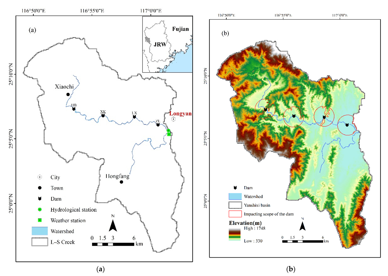
2.1. Study Area

The Longmen–Su (L–S) Creek represents the headwaters of the JRW, which is a combination of the Longmen Creek and Suxi Creek watersheds, with a drainage area of 132 km2 (Zhang et al., 2020) (Figure 1). The four cascaded small dams considered in this study were constructed in 2002; the basic information for these four dams is presented in Table 1. To measure the impact of damming on land cover and landscape patterns, we defined impact and non-impact areas in this study. The impacted area is defined as a 1.5 km buffer zone below 500 m elevation surrounding the dam reservoir zone, and the non-impacted area is classified as other areas in the L–S Creek.

2.2. Data Collection and Processing

The remote sensing image interpretation data included a 2.5 m resolution SPOT panchromatic image from 2004 and four phases of Landsat TM images from 2001, 2002, 2003, and 2004. Cloud cover was less than 1%. SPOT images were retrieved from the National Remote News World (http://www.ev-image.com/, accessed on 31 August 2017) and Landsat TM images were acquired from the Geospatial Data Cloud (http://www.gscloud.cn/, accessed on 31 August 2017). The image information used for land use classification is presented in Table S1.
After image preprocessing, including radiometric and atmospheric correction, we fused SPOT panchromatic images and Landsat TM images from 2004 to obtain multispectral and high-resolution data within the study area. Furthermore, the MNDWI index was used to extract the water body information. The water body image and the remaining image were extracted using a mask, and the remaining image land use change data were obtained through unsupervised classification and combined with visual interpretation. A complete land use classification result was obtained by mosaicking the two parts of the interpreted images. We assigned every cluster to one of five land categories and then compared the 2004 classification with the high-resolution image (8 m) from 2004, available on Google Earth. We collected 1250 purely random reference samples to assess accuracy and generated a confusion matrix, both in 2004 (Table S2); the accuracy between reference points and validation points in 2004 was 90.0%. There are five types of land use: water, woodlands, bareland, croplands, and built-up areas. Table S3 shows the land use classification system used in this study. Subsequently, we used the 2004 map to classify each preceding year in sequence. The process consisted of overlaying the map of 2004 on the 2003 image so that we could use visual interpretation to group pixels with the same characteristics. We repeated this procedure for 2002 and 2001 to produce a sequence of land cover maps for 2001, 2002, 2003, and 2004. The classification accuracy test used the overall accuracy and kappa coefficient to determine the classification accuracy. The interpretation accuracy of the interpretation results in the four years was higher than 90%, and the kappa coefficient was higher than 0.85. Having obtained high-precision watershed land use data, we delineated the spatial scope of the impact of the dam on the surrounding valley area below 1500 m above sea level based on the overall shape of the river and other factors (Figure 1). After obtaining the land use data, we conducted an enhanced intensity analysis and obtained landscape metrics to reveal the intensity changes and landscape patterns during the pre-impact, transition, and post-impact periods throughout the cascade dam construction. Finally, we explored and understood the relationship between changes in land use and landscape patterns and detailed implications for sustainability and planning. A methodological roadmap is shown in Figure 2.

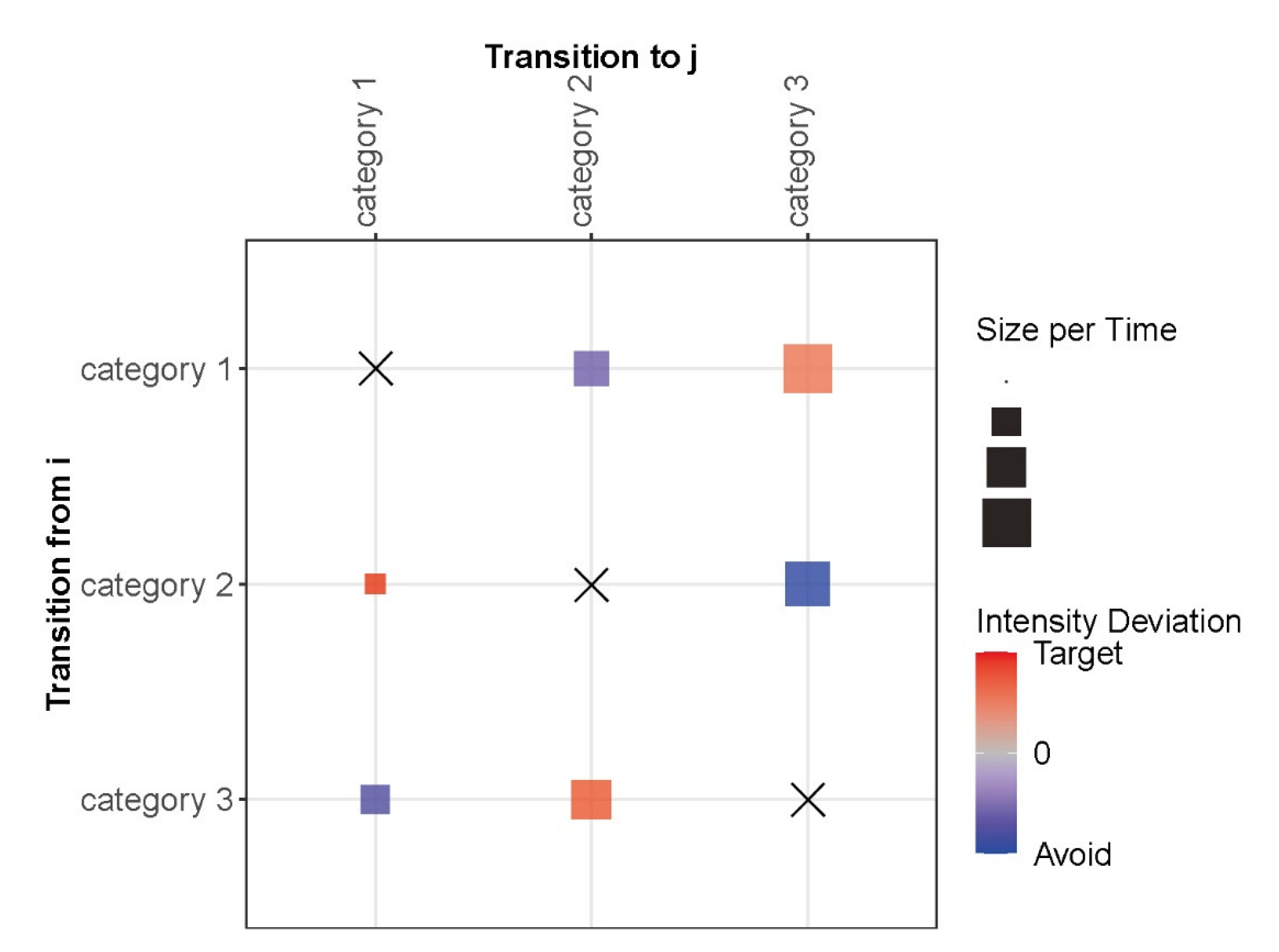
2.3. Enhanced Intensity Analysis

Intensity analysis is a hierarchical framework that compares uniform intensity to the observed intensities of temporal changes among categories [47,48]. Aldwaik and Pontius Jr. (2012) created an intensity analysis to dissect the transition matrices at three levels of detail: time interval, category, and transition. Supplementary Text S1 and Table S4 provide equations and notations for the three levels of detail [49].
An improved version of the intensity analysis method has been used to characterize land cover changes, mainly referring to the transition level. A cross-connected table of land conversion patterns named the “Transition pattern” was also used, as it can quickly and visually identify the intensity and area of land cover changes (Figure 3) [16].

2.4. Landscape Pattern Index
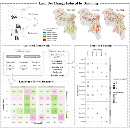
Landscape patterns in the impacted and non-impacted zones of the L–S Creek watershed were analyzed using two level-landscape and class-through landscape metrics, including Edge Density (ED), Area Mean (AREA_MN), Contagion Index (CONTAG), Shannon’s Diversity Index (SHDI), Landscape Shape Index (LSI), Largest Patch Index (LPI), and Interspersion Juxtaposition Index (IJI), for the years 2001–2004. Table S5 defines the mathematical symbols used in the equations and the descriptions of landscape metrics.

3. Results

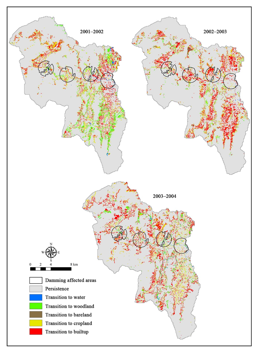
3.1. Overall Land Cover Changes

Figure 4 and Table S6 show the land use interpretation results for watershed land use from 2001–2004. Figure 5 presents maps of the five land categories at the four time points. During 2001–2004, 19.4% and 21.8% of the water area transitioned to woodland and built-up areas, respectively. Before and during the dam construction period (2001–2003), the built-up areas mostly transitioned to water. The gain in the woodland area mainly came from croplands, with a small part coming from bareland. The area of bareland in the watershed was relatively small; thus, the change in other land types to bareland was also relatively minor. In the three intervals, the 36% gain in cropland area mainly came from woodland; the rate of change from 24.3% of woodland area and 33.7% of cropland area to built-up area occupied the largest proportion of all land cover changes. In terms of the changing area affected by dams (Figure 5), water, bareland, and built-up areas increased from 2001–2004, while the woodland and cropland areas continued to decline. The cropland area showed the largest decrease, with transitions to water, woodland, and built-up areas. In the impacted area, the land cover change was mainly caused by the substantial increase in water (0.24 km2) and built-up areas (4.26 km2) and the decrease in woodlands (1.92 km2) and croplands (2.74 km2). A 0.17 km2 area of bareland steadily increased during construction. Comparing the changes in water bodies in the impacted areas during the two time periods, the water area increased, and the water capacity accumulated substantially in the upstream dams. It is noteworthy that the area of the water body increased by 0.18 ha (HB), 2.3 ha (XK), 0.27 ha (LX), and 3.2 ha (ZL) during the transition period. In the post-impact period, the water area increased by 6.55 ha (HB), 8.10 ha (XK), 6.35 ha (LX), and 9.79 ha (ZL).

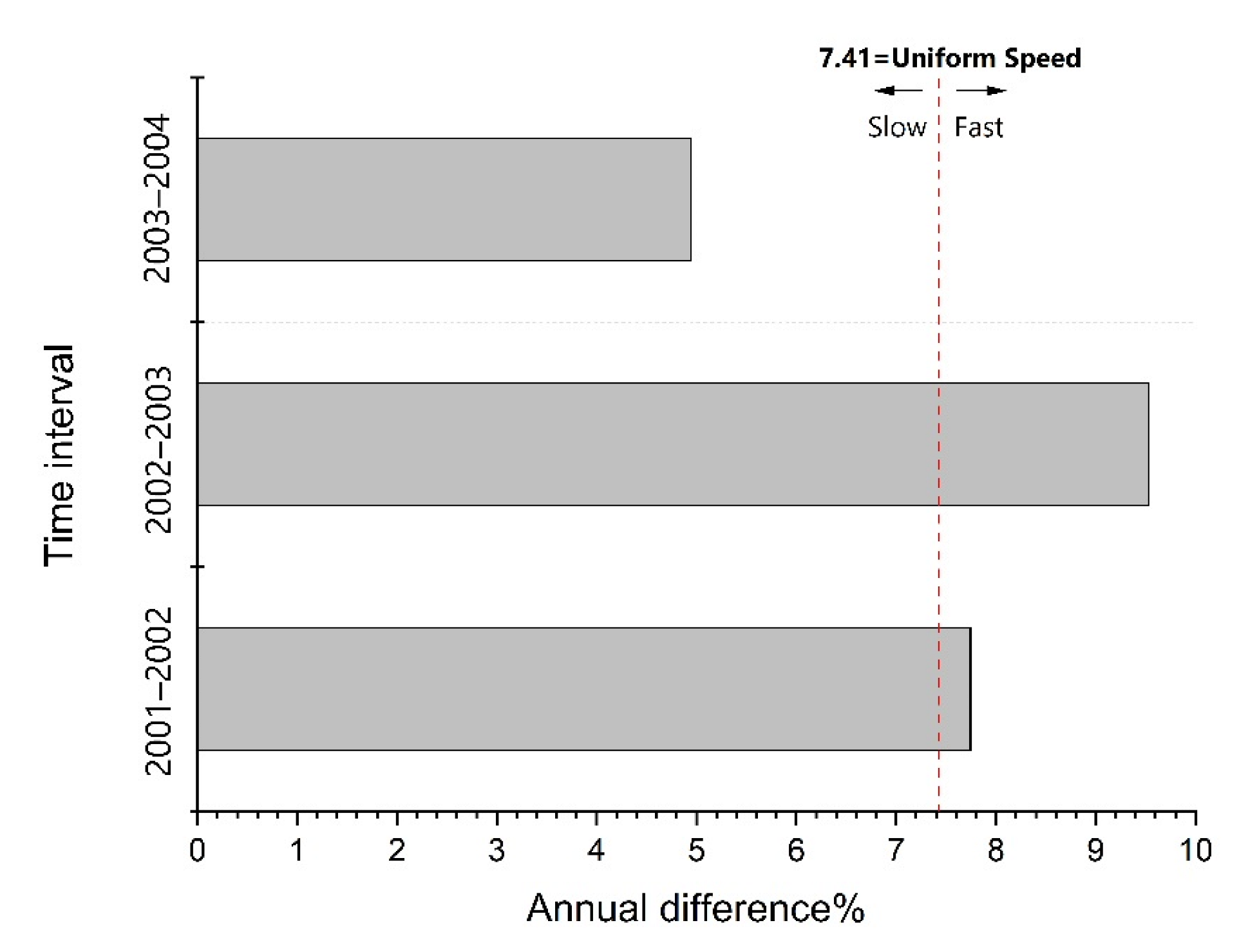
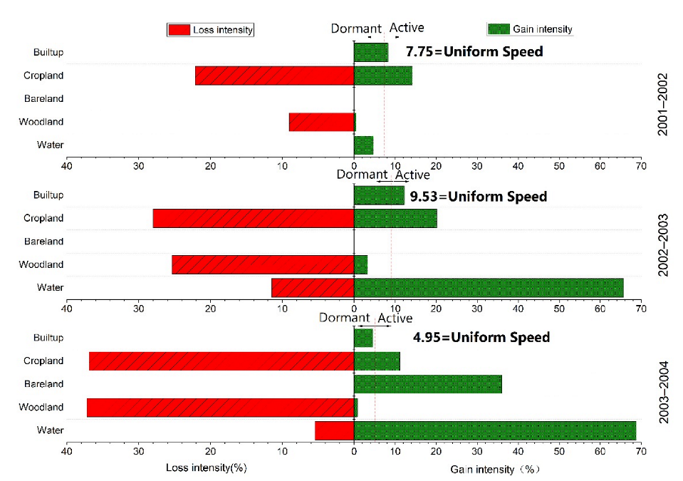
3.2. Change Analysis

Figure 6 and Figure S1 present maps of intensity changes during the three periods and LU/LC at the four time points in the impacted area of the L–S Creek watershed. The intensity of the land cover change during dam construction was greater than that of the other two intervals during 2002–2003.
Figure 7 shows the annual intensity of loss and gain as a percentage of the size of each category during the dam construction period. The annual differences were 4.95%, 9.53%, and 7.75% for the L–S Creek area during the three time intervals, respectively, which are identical to the annual differences in Figure 6. Figure 7 shows that the gains and losses of cropland and woodland were active, whereas the woodland gains and losses were dormant for all time intervals. The intensity of built-up gains increased during 2001–2003 owing to urbanization and dam construction. The intensities of water gains and losses increased during 2002–2003; however, the gain intensity of water was much higher than the loss intensity, indicating that dam construction can increase water accumulation in a river. Land cover changes within the range of cascade dam construction from 2002–2003 and 2003–2004 were visible, thus indicating that the dam construction period had a greater impact on the land use of small watersheds from the start to the end (Figure 7).
Figure 8 demonstrates the “transition pattern” during the three periods affected by dam construction in the L–S Creek watershed, thereby revealing the intensity and area changes at the transition level of intensity analysis. The increase in built-up areas mainly came at the expense of croplands, woodlands, and water. The conversion of croplands to built-up areas was the largest during 2002–2003 (during dam construction), although the gain in built-up areas was at the cost of croplands during all three time intervals. However, in 2001–2003, the gain in built-up areas did not come at the expense of woodlands, rather, in 2002–2004, this gain came from water. The increase in croplands was mainly derived from woodlands and the intensity change and area of croplands were the largest during 2002–2003. The area of bareland affected by dam construction was relatively small, and there were few changes. The increase in woodland area mainly came from croplands, with the highest area change and transition intensity occurring during 2002–2003. The increase in water was mainly at the expense of croplands, particularly during 2001–2003 (before and during dam construction). At the transition level, 0.7%, 4.5%, and 21.7% of woodlands were converted to croplands, water, and built-up areas, respectively. A proportion of croplands (8.1 %) was mainly converted to built-up areas, although 1.3% of croplands were converted to water. The increase in built-up land was the result of urbanization and the requirement for dam construction. Croplands are flooded or converted into built-up areas; however, these croplands have also been reclaimed and their area has increased. Owing to the dual effects of urbanization and dam construction, woodland loss was the most intensive.

3.3. Landscape Analysis

Landscape patterns in the impacted and non-impacted zones of the L–S Creek watershed were analyzed using two level-landscape and class-through landscape metrics, including ED, LSI, LPI, CONTAG, and SHDI, for 2001–2004. At the landscape level (Table 2), the landscape pattern changes in both zones showed the following characteristics. First, the overall ED was generally higher in impacted areas than in non-impacted areas because the construction-impacted area comprises four divided areas. In 2003, owing to the construction period of the dam, various types of patches underwent extraordinary transformation and integration; therefore, the ED value was low. The increase in the ED metric suggests that human disturbance resulted in a more fragmented landscape. Second, the decline in SHDI metrics in the impacted area suggests that the landscape has become less diverse. The landscape metric differences of ED, LSI, LPI, CONTAG, and SHDI between the two zones can be described as follows. First, the landscape patterns in the impacted zone were more fragmented and diverse with less connectivity. Second, the change rate of each metric was more intensive in the impacted zone.
During dam construction, the increase in built-up areas mainly occurred at the expense of croplands and woodlands. Therefore, the landscape pattern changes related to the land use classes of woodlands and croplands in the L–S Creek during 2001–2004 were further analyzed at the class level (Table 3), and the fragmentation of woodlands and croplands was explored using the ED metric. The similarity between the impacted and non-impacted zones was that the landscape of croplands became more fragmented owing to an increase in the ED value. The differences between the two zones were as follows. First, the LSI value of each category in the non-impacted zone was generally higher than that in the impacted zone. The LSI of bareland changed significantly before and after the dam’s construction. Second, AREA_MN in the non-dammed area was dominated by woodlands, peaked in 2003, and dropped sharply in 2004. Built-up areas dominated AREA_MN in the dam area, and its area increased sharply from 2002–2003. Third, from the perspective of connectivity, the non-impacted zone was dominated by natural landscapes and the connectivity of each category was generally high. The IJI of the water body before and after the impacted zone in the dam-building area dropped significantly, especially during the dam-building period in 2003, when it reached its lowest value.

3.4. Relationship between the Intensity of Land Use Changes and Landscape Pattern Dynamics Induced by Damming

Based on the observations of the four dam construction areas, the overall change intensity and area of land use, the change rate of landscape pattern metrics at three time intervals, and the relationship between the changing intensity of land use and landscape pattern change are shown in Figure 9. The results show that the water land use area change rate is strongly negatively correlated with LPI (−0.55 *), IJI (−0.57 *), and ED (−0.55 *), and the water land use intensity change rate is strongly negatively correlated with LPI (−0.58 *) and ED (−0.63 *), thereby implying that a faster gain in water is associated with a more fragmented water landscape. The woodland intensity change rate of land use was strongly positively correlated with AREA_MN (0.57 *) in the impacted zone, whereas it was associated with greater heterogeneity of the overall landscape pattern.

4. Discussion

4.1. Effectiveness of the Proposed Framework in a Small Headwater Watershed

It is well documented that LU/LC changes can be caused by cascade dam construction [17,50,51]. However, specific impacts on land cover change during different periods of dam construction have seldom been reported. Our framework offers insights into how to measure damming impacts on land cover and landscape patterns in small watersheds. Our proposed framework is a collection of tools that can help scientists consider whether dam construction can explain rapid changes in land use and landscape patterns. Specifically, Figure 8 shows the “transition pattern” during the three construction periods, which can be used to reveal the results quickly and to visually identify the intensity and area of land cover change. Xie et al. (2020) found similar results of land change by “transition pattern” caused by rapid urbanization in Nanchang, China. Table 2 and Table 3 show the different changes in landscape and class between impacted and non-impacted areas in this study [16]. Tang et al. (2020) showed that the change rate of each metric is more intensive in the estuary zone [52]. This finding is consistent with the results of the present study.
Although it was found that China’s land consolidation project and afforestation programs could convert some land from built to cropland and from cropland to woodland [53], we admit that data errors might account for some of the apparent anomalous transitions, that is, from built-up areas to croplands or from croplands to forests in a short time, as shown in Figure S1. We have seen this same transition in other datasets, specifically GlobeLand30 [48]. It may be difficult for classifiers of remotely sensed images to differentiate between built and cropland, cropland, and woodland, especially when the two categories exist close to each other as they frequently do in Asia.

4.2. Linking Land Cover Change with Landscape Pattern Dynamics Induced by Damming

Intensity analysis is a viable method for linking patterns to land change processes [35,37,54,55]. In this case, the land cover change pattern reflects the impact of dam construction on the land cover in the region. At the transition level, the largest transitions to built-up areas are derived from croplands and woodlands, whereas water gains are mostly from croplands (Figure 8). As croplands have been flooded or converted into built-up areas, reclamation has also increased. Owing to urbanization and dam construction, the loss of woodlands and increase in water areas are remarkable, and these results are similar to those of other observations [6,11]. In terms of the changing area during the post-impact period, the upstream water area increased significantly, whereas the downstream water area decreased. These changes may have led to soil loss and increased river sediment and nutrient levels [20]. According to the analysis of the intensity of land cover change in this study, the intensity change of bareland is not very active, which is likely caused by woodland spread during dam construction [51].
Our intensity analysis for land cover change revealed that the transition from cropland to water area was intensive in the L–S Creek watershed. Figure 9 shows that greater water loss is associated with increased fragmentation in the impact zone. This is consistent with previous studies that argue that the degree of hydrologic alteration is significantly correlated with landscape metric changes, especially for forested and water areas in and surrounding the Lancang River in Yunnan Province, China [4,56]. Furthermore, Figure 9 also shows that a faster gain in cropland is associated with a more heterogeneous landscape in the impacted zone. Su et al. (2014) argued that increases in fragmentation and isolation were identified for all vegetated landscape types disturbed by anthropogenic activities in the Tiaoxi watershed of Zhejiang Province, China, which is similar to our results for the impacted area [57]. In addition, the degree of land use change intensity was strongly correlated with the degree of landscape fragmentation and heterogeneity in the impacted zone, which is consistent with the results in the state of Selangor on the west coast of peninsular Malaysia [58].

4.3. Implications for Land Management

Environmental impacts stemming from dam construction extend to the entire river basin, including changes from altered sediment and water flows as well as losses of aquatic fauna and losses or disturbances of vast areas of forests, floodplains, and other ecosystems [21,59,60,61]. Our research has used efficient methods to reveal land cover changes in small watersheds before and after dam construction and analyzed the transition pattern between land use types through intensity analysis, thereby providing ideas for monitoring land cover changes caused by dam construction. Land cover change during the dam construction period was visible in the impacted area, and there were notable reductions in croplands and woodlands. Encroachment into croplands by dam construction affects the interests of residents, farmers, and local agricultural activities which underscores the need to compensate farmers for their economic losses and maintain regional food production by other means [62,63]. A substantial portion of the gain in built-up areas was derived from woodlands, which increased the risk of soil erosion in this small watershed. A change in the subsurface properties also leads to a change in the surface water storage capacity, with a decrease in infiltration during heavy rainfall and an increase in surface runoff. This increases the water level of the rivers after damming and increases the area of water bodies but also aggravates the problem of non-point source pollution [21,60]. In other words, during and following dam construction, land use on both sides of the riverbank requires monitoring to avoid excessive woodland loss, which reduces soil erosion in small watersheds. If the dam construction time is too concentrated, the land use area will change enormously, making the small watershed ecosystem vulnerable to external disturbances and damage within the impacted area [59]. Therefore, concentrated dam construction activities over a short period should be avoided as much as possible.
Mega construction projects have a great capacity to change landscapes and socio-ecological systems, which are potentially damaging in developing regions [9]. The impact of damming activities on the overall landscape pattern of a small watershed can be illustrated macroscopically [64]. Damming affects the fragmentation, heterogeneity, and connectivity of land use within the impacted area, which places specific requirements on the scale and structure of dam construction [52]. Foremost, dam construction should minimize the impact of human activities on nature by not destroying natural patches and ensuring the connectivity of land types. Conversely, an appropriate amount of damming can regulate the hydrological conditions of a small watershed, increase the heterogeneity of land use within the impacted area, and promote overall landscape diversity. More in-depth studies are required to investigate how to coordinate the scale and location of dam construction sites to achieve the best landscape pattern optimization.

5. Conclusions

We developed a framework to reveal changes in LU/LC and landscapes induced by dam construction in a small watershed. Land use in the L–S Creek watershed changed vigorously during the transition and post-impact periods of dam construction. The intensity of land cover change within the damming construction was the highest among the three periods, indicating that dam construction caused the land cover change. This change was mainly caused by the substantial increase in water and built-up areas and a decrease in woodlands and croplands. The amount of bBareland steadily increased during construction. Driven by damming, 21.7% of woodlands and 8.1% of croplands were converted to built-up areas, and 0.7% of woodlands and 1.3% of croplands were flooded or transformed into water bodies. By linking land cover change with landscape patterns, land use change in water was significantly associated with landscape fragmentation and heterogeneity in the impacted area. Therefore, monitoring of land cover change should be strengthened during and after dam construction to prevent soil erosion and non-point source pollution.

Supplementary Materials

The following supporting information can be downloaded at https://www.mdpi.com/article/10.3390/rs14153580/s1, Text S1: Three levels of intensity analysis; Table S1: Image information used for land use classification; Table S2: Error matrix of the land cover classification accuracy assessment in 2004; Table S3: Land use classification system; Table S4: Mathematical notation; Table S5: Equations and descriptions of landscape metrics; Table S6: Land use area during 2001–2004; Figure S1: Land use/land cover in the impacted area.

Author Contributions

Conceptualization, Z.X. and J.H.; Data curation, J.L. and Z.C.; Investigation, Z.C.; Methodology, J.H.; Visualization, Z.X.; Writing—original draft, Z.X.; Writing—review and editing, J.H. and X.L. All authors have read and agreed to the published version of the manuscript.

Funding

This research was funded by the National Natural Science Foundation of China (grant numbers 41971231 and 41471154) and China Scholarship Council (grant number 202106310078).

Data Availability Statement

Not applicable.

Conflicts of Interest

The authors declare no conflict of interest.

References

  1. Grill, G.; Lehner, B.; Thieme, M.; Geenen, B.; Tickner, D.; Antonelli, F.; Babu, S.; Borrelli, P.; Cheng, L.; Crochetiere, H.; et al. Mapping the world’s free-flowing rivers. Nature 2019, 569, 215–221. [Google Scholar] [CrossRef] [PubMed]
  2. Barbarossa, V.; Schmitt, R.J.P.; Huijbregts, M.A.J.; Zarfl, C.; King, H.; Schipper, A.M. Impacts of current and future large dams on the geographic range connectivity of freshwater fish worldwide. Proc. Natl. Acad. Sci. USA 2020, 117, 3648–3655. [Google Scholar] [CrossRef] [PubMed] [Green Version]
  3. Maavara, T.; Akbarzadeh, Z.; Van Cappellen, P. Global dam-driven changes to riverine N:P:si ratios delivered to the coastal ocean. Geophys. Res. Lett. 2020, 47, e2020. [Google Scholar] [CrossRef]
  4. Zhang, Z.; Liu, J.; Huang, J. Hydrologic impacts of cascade dams in a small headwater watershed under climate variability. J. Hydrol. 2020, 590, 125426. [Google Scholar] [CrossRef]
  5. Ouyang, W.; Hao, F.; Song, K.; Zhang, X. Cascade dam-induced hydrological disturbance and environmental impact in the upper stream of the Yellow River. Water Resour. Manag. 2011, 25, 913–927. [Google Scholar] [CrossRef]
  6. Li, K.; Zhu, C.; Wu, L.; Huang, L. Problems caused by the Three Gorges Dam construction in the Yangtze River basin: A review. Environ. Rev. 2013, 21, 127–135. [Google Scholar] [CrossRef]
  7. Li, Y.; Hu, J.; Han, X.; Li, Y.; Li, Y.; He, B.; Duan, X. Effects of past land use on soil organic carbon changes after dam construction. Sci. Total Environ. 2019, 686, 838–846. [Google Scholar] [CrossRef]
  8. Yang, J.; Shi, F.; Sun, Y.; Zhu, J. A cellular automata model constrained by spatiotemporal heterogeneity of the urban development strategy for simulating land use change: A Case study in Nanjing City, China. Sustainability 2019, 11, 4012. [Google Scholar] [CrossRef] [Green Version]
  9. Calvi, M.F.; Moran, E.F.; da Silva, R.F.B.; Batistella, M. The construction of the Belo Monte dam in the Brazilian Amazon and its consequences on regional rural labor. Land Use Policy 2020, 90, 104327. [Google Scholar] [CrossRef]
  10. Liu, Y.; Yang, W.; Yu, Z.; Lung, I.; Yarotski, J.; Elliott, J.; Tiessen, K. Assessing effects of small dams on stream flow and water quality in an agricultural watershed. J. Hydrol. Eng. 2014, 19, 5014015. [Google Scholar] [CrossRef]
  11. Bhatti, N.B.; Siyal, A.A.; Qureshi, A.L.; Bhatti, I.A. Land covers change assessment after small Dam’s construction based on the satellite data. Civ. Eng. J. 2019, 5, 810–818. [Google Scholar] [CrossRef] [Green Version]
  12. Turner, B.L.; Robbins, P. Land-change science and political ecology: Similarities, differences, and implications for sustainability science. Annu. Rev. Environ. Resour. 2008, 33, 295–316. [Google Scholar] [CrossRef]
  13. Alturk, B.; Konukcu, F. Modeling land use/land cover change and mapping morphological fragmentation of agricultural lands in Thrace Region/Turkey. Environ. Dev. Sustain. 2020, 22, 6379–6404. [Google Scholar] [CrossRef]
  14. Lambin, E.F.; Meyfroidt, P. Global land use change, economic globalization, and the looming land scarcity. Proc. Natl. Acad. Sci. USA 2011, 108, 3465–3472. [Google Scholar] [CrossRef] [Green Version]
  15. IPCC. Climate Change, Desertification, Land Degradation, Sustainable Land Management, Food Security, and Greenhouse Gas Fluxes in Terrestrial Ecosystems; Cambridge University Press: London, UK, 2019. [Google Scholar]
  16. Xie, Z.; Pontius, R.G., Jr.; Huang, J.; Nitivattananon, V. Enhanced intensity analysis to quantify categorical change and to identify suspicious land transitions: A Case study of Nanchang, China. Remote Sens. 2020, 12, 3323. [Google Scholar] [CrossRef]
  17. Jiang, X.; Lu, D.; Moran, E.; Calvi, M.F.; Dutra, L.V.; Li, G. Examining impacts of the Belo Monte hydroelectric dam construction on land cover changes using multitemporal Landsat imagery. Appl. Geogr. 2018, 97, 35–47. [Google Scholar] [CrossRef]
  18. Eekhout, J.P.C.; Boix-Fayos, C.; Pérez-Cutillas, P.; de Vente, J. The impact of reservoir construction and changes in land use and climate on ecosystem services in a large Mediterranean catchment. J. Hydrol. 2020, 590, 125208. [Google Scholar] [CrossRef]
  19. Nnaji, C.C.; Ogarekpe, N.M.; Nwankwo, E.J. Temporal and spatial dynamics of land use and land cover changes in derived savannah hydrological basin of Enugu State, Nigeria. Environ. Dev. Sustain. 2022, 24, 9598–9622. [Google Scholar] [CrossRef]
  20. Rodrigues, L.N.; Sano, E.E.; Steenhuis, T.S.; Passo, D.P. Estimation of small reservoir storage capacities with remote sensing in the Brazilian savannah region. Water Resour. Manag. 2012, 26, 873–882. [Google Scholar] [CrossRef]
  21. Cho, M.S.; Qi, J. Quantifying spatiotemporal impacts of hydro-dams on land use/land cover changes in the Lower Mekong River Basin. Appl. Geogr. 2021, 136, 102588. [Google Scholar] [CrossRef]
  22. Chen, X.; Wang, Y.; Cai, Z.; Zhang, M.; Ye, C. Response of the nitrogen load and its driving forces in estuarine water to dam construction in Taihu Lake, China. Environ. Sci. Pollut. Res. Int. 2020, 27, 31458–31467. [Google Scholar] [CrossRef]
  23. McFeeters, S.K. The use of the Normalized Difference Water Index (NDWI) in the delineation of open water features. Int. J. Remote Sens. 1996, 17, 1425–1432. [Google Scholar] [CrossRef]
  24. Xu, H. Modification of normalised difference water index (NDWI) to enhance open water features in remotely sensed imagery. Int. J. Remote Sens. 2006, 27, 3025–3033. [Google Scholar] [CrossRef]
  25. Luo, J.; Sheng, Y.; Shen, Z.; Li, J.; Gao, L. Automatic and high-precise extraction for water information from multispectral images with the step-by-step iterative transformation mechanism Automatic and high-precise extraction for water information from multispectral images with the step-by-step iterative transformation mechanism. J. Remote Sens. 2009, 13, 610–615. [Google Scholar]
  26. Yang, S.; Xue, C.; Liu, T.; Li, Y. A method of small water information automatic extraction from TM remote sensing images. Acta Geod. Cartogr. Sin. 2010, 39, 611–617. [Google Scholar]
  27. Du, J.; Huang, Y.; Feng, X.; Wang, Z. Study on water bodies extraction and classification from SPOT image. J. Remote Sens. 2001, 5, 214–219. [Google Scholar]
  28. Deng, J.; Wang, K.; Li, J.; Dong, Y. Study on the automatic extraction of water body informat ion from SPOT-5 images using decision tree algorithm. J. Zhejiang Univ. (Agric. Life Sci.) 2005, 31, 171–174. [Google Scholar]
  29. Zheng, C.; Wang, X.; Huang, J. Decision tree algorithm of automatically extracting paddy rice Information 5from SPOT-5 Images Based on Characteristic Bands. Remote Sens. Technol. Appl. 2008, 23, 294–299. [Google Scholar]
  30. Wei, X.; Sauvage, S.; Ouillon, S.; Le, T.P.Q.; Orange, D.; Herrmann, M.; Sanchez-Perez, J.-M. A modelling-based assessment of suspended sediment transport related to new damming in the Red River basin from 2000 to 2013. CATENA 2021, 197, 104958. [Google Scholar] [CrossRef]
  31. Versace, V.L.; Ierodiaconou, D.; Stagnitti, F.; Hamilton, A.J. Appraisal of random and systematic land cover transitions for regional water balance and revegetation strategies. Agric. Ecosyst. Environ. 2008, 123, 328–336. [Google Scholar] [CrossRef]
  32. Shoyama, K.; Braimoh, A.K. Analyzing about sixty years of land cover change and associated landscape fragmentation in Shiretoko Peninsula, Northern Japan. Landsc. Urban Plan. 2011, 101, 22–29. [Google Scholar] [CrossRef]
  33. Romero-Ruiz, M.H.; Flantua, S.G.A.; Tansey, K.; Berrio, J.C. Landscape transformations in savannas of northern South America: Land use/cover changes since 1987 in the Llanos Orientales of Colombia. Appl. Geogr. 2012, 32, 766–776. [Google Scholar] [CrossRef]
  34. Quan, B.; Pontius, R.G., Jr.; Song, H. Intensity Analysis to communicate land change during three time intervals in two regions of Quanzhou City, China. Remote Sens. 2020, 57, 21–36. [Google Scholar] [CrossRef]
  35. Pontius, R.G., Jr.; Gao, Y.; Giner, N.M.; Kohyama, T.; Osaki, M.; Hirose, K. Design and interpretation of intensity analysis illustrated by land change in Central Kalimantan, Indonesia. Land 2013, 2, 351–369. [Google Scholar] [CrossRef]
  36. Zhou, P.; Huang, J.; Pontius, R.G., Jr.; Hong, H. Land classification and change intensity analysis in a coastal watershed of Southeast China. Sensors 2014, 14, 11640–11658. [Google Scholar] [CrossRef] [Green Version]
  37. Huang, J.; Pontius, R.G., Jr.; Li, Q.; Zhang, Y. Use of intensity analysis to link patterns with processes of land change from 1986 to 2007 in a coastal watershed of southeast China. Appl. Geogr. 2012, 34, 371–384. [Google Scholar] [CrossRef]
  38. Renetzeder, C.; Schindler, S.; Peterseil, J.; Prinz, M.A.; Mücher, S.; Wrbka, T. Can we measure ecological sustainability? Landscape pattern as an indicator for naturalness and land use intensity at regional, national and European level. Ecol. Indic. 2010, 10, 39–48. [Google Scholar] [CrossRef]
  39. Estoque, R.C.; Murayama, Y. Quantifying landscape pattern and ecosystem service value changes in four rapidly urbanizing hill stations of Southeast Asia. Landsc. Ecol. 2016, 31, 1481–1507. [Google Scholar] [CrossRef]
  40. Kienast, F.; Frick, J.; van Strien, M.J.; Hunziker, M. The Swiss Landscape Monitoring Program—A comprehensive indicator set to measure landscape change. Ecol. Modell. 2015, 295, 136–150. [Google Scholar] [CrossRef]
  41. Wan, L.; Zhang, Y.; Zhang, X.; Qi, S.; Na, X. Comparison of land use/land cover change and landscape patterns in Honghe National Nature Reserve and the surrounding Jiansanjiang Region, China. Ecol. Indic. 2015, 51, 205–214. [Google Scholar] [CrossRef]
  42. Cao, K. Spatial-temporal dynamics analysis of coastal landscape pattern on driving force of human activities: A case in south Yingkou, China. Appl. Ecol. Environ. Res. 2017, 15, 923–937. [Google Scholar] [CrossRef]
  43. Huang, J.; Huang, Y.; Pontius, R.G.; Zhang, Z. Geographically weighted regression to measure spatial variations in correlations between water pollution versus land use in a coastal watershed. Ocean Coast. Manag. 2015, 103, 14–24. [Google Scholar] [CrossRef]
  44. Huang, J.; Zhang, Z.; Feng, Y.; Hong, H. Hydrologic response to climate change and human activities in a subtropical coastal watershed of southeast China. Reg. Environ. Chang. 2013, 13, 1195–1210. [Google Scholar] [CrossRef]
  45. Zhang, Z.; Huang, J.; Huang, Y.; Hong, H. Streamflow variability response to climate change and cascade dams development in a coastal China watershed. Coast. Shelf Sci. 2015, 166, 209–217. [Google Scholar] [CrossRef]
  46. Lu, W.; Lei, H.; Yang, D.; Tang, L.; Miao, Q. Quantifying the impacts of small dam construction on hydrological alterations in the Jiulong River basin of Southeast China. J. Hydrol. 2018, 567, 382–392. [Google Scholar] [CrossRef]
  47. Teixeira, Z.; Marques, J.C.; Pontius, R.G. Evidence for deviations from uniform changes in a Portuguese watershed illustrated by CORINE maps: An Intensity Analysis approach. Ecol. Indic. 2016, 66, 382–390. [Google Scholar] [CrossRef] [Green Version]
  48. Shafizadeh-Moghadam, H.; Minaei, M.; Feng, Y.; Pontius, R.G., Jr. GlobeLand30 maps show four times larger gross than net land change from 2000 to 2010 in Asia. Int. J. Appl. Earth Obs. Geoinf. 2019, 78, 240–248. [Google Scholar] [CrossRef]
  49. Aldwaik, S.Z.; Pontius, R.G., Jr. Intensity analysis to unify measurements of size and stationarity of land changes by interval, category, and transition. Landsc. Urban Plan. 2012, 106, 103–114. [Google Scholar] [CrossRef]
  50. Chen, Z.; Wang, J. Land use and land cover change detection using satellite remote sensing techniques in the mountainous Three Gorges Area, China. Int. J. Remote Sens. 2010, 31, 1519–1542. [Google Scholar] [CrossRef]
  51. Iwuji, M.C.; Iheanyichukwu, C.P.; Njoku, J.D.; Okpiliya, F.I.; Anyanwu, S.O.; Amangabara, G.T.; Ukaegbu, K.O.E. Assessment of land use changes and impacts of dam construction on the Mbaa River, Ikeduru, Nigeria. JGEESI 2017, 13, 1–10. [Google Scholar] [CrossRef]
  52. Tang, J.; Li, Y.; Cui, S.; Xu, L.; Ding, S.; Nie, W. Linking land use change, landscape patterns, and ecosystem services in a coastal watershed of southeastern China. Glob. Ecol. Conserv. 2020, 23, e01177. [Google Scholar] [CrossRef]
  53. Yu, Q.; Hu, Q.; van Vliet, J.; Verburg, P.H.; Wu, W. GlobeLand30 shows little cropland area loss but greater fragmentation in China. Int. J. Appl. Earth Obs. Geoinf. ITC J. 2018, 66, 37–45. [Google Scholar] [CrossRef]
  54. Huang, B.; Huang, J.; Gilmore Pontius, R.G., Jr.; Tu, Z. Comparison of Intensity Analysis and the land use dynamic degrees to measure land changes outside versus inside the coastal zone of Longhai, China. Ecol. Indic. 2018, 89, 336–347. [Google Scholar] [CrossRef]
  55. Pontius, R.G., Jr. Component intensities to relate difference by category with difference overall. Int. J. Appl. Earth Obs. Geoinf. 2019, 77, 94–99. [Google Scholar] [CrossRef]
  56. Zhao, Q.; Liu, S.; Deng, L.; Dong, S.; Cong, W.; Wang, Z.; Yang, Z.; Yang, J. Landscape change and hydrologic alteration associated with dam construction. Int. J. Appl. Earth Obs. Geoinf. 2012, 16, 17–26. [Google Scholar] [CrossRef]
  57. Su, S.; Ma, X.; Xiao, R. Agricultural landscape pattern changes in response to urbanization at ecoregional scale. Ecol. Indic. 2014, 40, 10–18. [Google Scholar] [CrossRef]
  58. Abdullah, A.Y.M.; Masrur, A.; Adnan, M.S.G.; Baky, M.A.A.; Hassan, Q.K.; Dewan, A. Spatio-temporal patterns of land use/land cover change in the heterogeneous coastal region of Bangladesh between 1990 and 2017. Remote Sens. 2019, 11, 790. [Google Scholar] [CrossRef] [Green Version]
  59. Fearnside, P.M. Environmental and social impacts of hydroelectric dams in Brazilian Amazonia: Implications for the aluminum industry. World Dev. 2016, 77, 48–65. [Google Scholar] [CrossRef]
  60. Lupinacci, C.M.; da Conceição, F.T.; Heck Simon, A.L.; Perez Filho, A. Land use changes due to energy policy as a determining factor for morphological processes in fluvial systems in São Paulo State, Brazil. Earth Surf. Process. Landforms 2017, 42, 2402–2413. [Google Scholar] [CrossRef]
  61. Tao, Y.; Wang, H.; Ou, W.; Guo, J. A land cover-based approach to assessing ecosystem services supply and demand dynamics in the rapidly urbanizing Yangtze River Delta region. Land Use Policy 2018, 72, 250–258. [Google Scholar] [CrossRef]
  62. Cheng, L.; Brown, G.; Liu, Y.; Searle, G. An evaluation of contemporary China’s land use policy—The Link Policy: A case study from Ezhou, Hubei Province. Land Use Policy 2020, 91, 104423. [Google Scholar] [CrossRef]
  63. Liu, Y.; Fang, F.; Li, Y. Key issues of land use in China and implications for policy making. Land Use Policy 2014, 40, 6–12. [Google Scholar] [CrossRef]
  64. Castello, L.; Macedo, M.N. Large-scale degradation of Amazonian freshwater ecosystems. Glob. Chang. Biol. 2016, 22, 990–1007. [Google Scholar] [CrossRef]
Figure 1. Location of the study area (a) and impacted area of dam construction in the L–S Creek (b).
Remotesensing 14 03580 g001
Figure 2. Methodological road map.
Remotesensing 14 03580 g002
Figure 3. Structure of transition pattern. The intensity deviation refers to the deviation between the transition intensity Rtij of a specific off-diagonal entry and the column’s uniform transition intensity Wtj. The supplementary materials section provides the equations for Rtij and Wtj. Readers should compare the colors within a column to see how each column gains category targets or avoids each row’s losing category. “×” means no transition between the same land use types during two periods.
Remotesensing 14 03580 g003
Figure 4. Maps of land categories in the L–S Creek watershed during 2001–2004.
Remotesensing 14 03580 g004
Figure 5. Land cover change analysis during three time intervals.
Remotesensing 14 03580 g005
Figure 6. Intensity changes during three time intervals in L–S Creek watershed.
Remotesensing 14 03580 g006
Figure 7. Category-level intensity analysis for the three time intervals.
Remotesensing 14 03580 g007
Figure 8. Transition patterns for three time intervals. The gradient of colors indicates the deviation between the intensity of the gain of each column category and the uniform transition intensity. Intensity Deviation = Rtij − Wtj. “×” means no transition between the same land use types during two periods.
Remotesensing 14 03580 g008
Figure 9. Correlation between the change intensity of land use and landscape patterns. Significant different (*) means p < 0.05.
Remotesensing 14 03580 g009
Table 1. Small dam information in the L–S Creek watershed [4].
NameCapacity (103 m3)Drainage Area (km2)TypeConstruction Year
Hejiabi (HB)195.50.8Flood Dam2003
Xikengkou (XK)820.4Hydropower Dam2003
Longmenxi (LX)27.40.2Hydropower Dam2003
Zhaolong (ZL)820.5Hydropower Dam2003
Table 2. Landscape pattern change in the L–S Creek watershed.
EDLSILPICONTAGSHDI
OutsideInsideOutsideInsideOutsideInsideOutsideInsideOutsideInside
200161.23119.3531.1318.2454.9420.0470.2559.310.761.10
200263.31103.4232.1016.2754.5122.5771.0748.170.741.11
200355.5992.2328.5214.8852.4023.3570.4362.220.770.94
200465.42122.6633.0818.6547.6021.4071.5662.220.810.99
Outside and inside represent non-impacted and impacted areas, respectively.
Table 3. Landscape pattern changes of various land use types in the L–S Creek watershed.
EDLSILPIAREA_MNIJI
LIDTYPEOutsideInsideOutsideInsideOutsideInsideOutsideInsideOutsideInside
2001Water2.3916.3525.1718.960.080.362.003.4664.9552.28
Woodland30.0243.1018.6412.5554.9411.62173.0216.8561.1855.61
Bareland0.820.379.582.140.020.021.390.5410.8836.03
Cropland43.6484.8660.6324.901.743.225.682.8850.1243.01
Builtup45.5994.0357.6819.067.1420.048.5914.0055.1853.50
2002Water2.7619.2521.7314.830.110.882.554.0974.0876.77
Woodland32.3640.9619.7312.1154.518.87114.0217.1952.6669.87
Bareland0.02-1.39-0.01-1.82-66.56-
Cropland50.4276.8677.5824.820.463.212.973.0653.6878.45
Builtup41.0569.7750.4214.146.2522.5710.5422.9051.7481.84
2003Water2.6417.2223.4518.530.080.462.222.3351.8731.29
Woodland27.7235.3117.6411.4452.409.04218.0222.4758.5555.30
Bareland1.19-9.82-0.15-3.35-76.23-
Cropland40.8959.0978.3527.180.130.271.621.0752.9351.31
Builtup38.7472.8639.5713.247.9523.3521.5154.2761.7471.86
2004Water2.8516.4119.7714.200.150.663.015.6852.3046.33
Woodland38.4054.9323.7816.2247.604.4283.616.5648.2648.54
Bareland2.954.7321.817.180.010.100.710.8660.5061.66
Cropland30.4560.5867.7226.990.090.351.160.9436.7326.38
Builtup55.73108.6850.9119.008.0321.4020.4339.4455.8762.89
Outside and inside represent non-impacted and impacted areas, respectively.
Publisher’s Note: MDPI stays neutral with regard to jurisdictional claims in published maps and institutional affiliations.

