Abstract
To ensure future food security, improved agricultural management approaches are required. For many of those applications, precise knowledge of the distribution of crop types is essential. Various machine and deep learning models have been used for automated crop classification using microwave remote sensing time series. However, the application of these approaches on a large spatial and temporal scale is barely investigated. In this study, the performance of two frequently used algorithms, Long Short-Term Memory (LSTM) networks and Random Forest (RF), for crop classification based on Sentinel-1 time series and meteorological data on a large spatial and temporal scale is assessed. For data from Austria, the Netherlands, and France and the years 2015–2019, scenarios with different spatial and temporal scales were defined. To quantify the complexity of these scenarios, the Fisher Discriminant measurement F1 (FDR1) was used. The results demonstrate that both classifiers achieve similar results for simple classification tasks with low FDR1 values. With increasing FDR1 values, however, LSTM networks outperform RF. This suggests that the ability of LSTM networks to learn long-term dependencies and identify the relation between radar time series and meteorological data becomes increasingly important for more complex applications. Thus, the study underlines the importance of deep learning models, including LSTM networks, for large-scale applications.
1. Introduction
Food supply is one of the biggest challenges of the 21st century. Presently, there are already 820 million people suffering from malnutrition [1]. Two driving forces are expected to aggravate this trend in the next decades. First, the world population is growing profusely, with potentially 9.7 billion people in 2050 [2]. The populace of sub-Saharan Africa, a region often threatened by hunger, is expected to double by 2050 [2]. Second, due to global warming, precipitation patterns will change in many regions, and the average temperatures will increase. As a result, seasonal crop failures and permanent loss of arable land due to desertification are expected to occur more often [3]. To counteract these factors, more advanced agricultural monitoring applications are needed. Remote sensing applications developed in this context include yield prediction, irrigation models, and forecasts of production loss [4,5,6]. However, to deliver accurate results, these applications require precise knowledge about the distribution and location of crop types. For time and cost reasons, it is also important that the applied models not only work locally and for a limited time scale, but on a country level or even several countries. Moreover, the model must be applicable to upcoming years. Remote sensing provides a timely and large-scale overview of conditions on the ground and is therefore suitable for this purpose. New satellite generations provide data of both a high temporal and a large spatial scale. An example is the Copernicus Sentinel-1 mission with currently two identical synthetic aperture radar (SAR) satellites that offer seamless, dense time series thanks to the sensor and mission-specific properties. In addition, the C-band SAR instrument is sensitive to vegetation properties and thus able to derive information on the growing stage and plant structure which can be used for crop classification [7,8,9,10]. The availability of large amounts of data has also led to the increasing popularity of automated evaluation procedures. In particular, the field of machine learning (ML) opened up new possibilities for automated discrimination of crop types.
1.1. Machine Learning Based Crop Classification
A large number of studies exist that evaluate different classifiers for SAR time series based crop classification. A wide range of classifiers have already been evaluated: Xu et al. [11] used K-Mean clustering and spectral similarity values for crop classification. Tan et al. [12] used an entropy decomposition and a Support Vector Machine for crop classification in the Netherlands. Kenduiywoa et al. [13] employed an ensemble of Random Forest (RF) classifiers on SAR time series. Ustuner et al. [14] analyzed different Gradient Boosting approaches with C-band data to classify crops in Turkey. All studies achieved overall accuracies around 90% and demonstrated the general suitability of machine learning and C-band radar time series for crop classification. Nitze et al. [15] compared multiple common ML classifiers and concluded that they achieve comparable results if applied on multiple images (a time series). However, all cited studies only focused on a single year and country. Orynbaikyzy et al. [16] reviewed 75 publications using optical and radar sensor fusion for crop classification and identified only one study that focused on an area larger than 500,000 km2. Yet, this particular study from Torbick et al. [17] only focused on a single crop type (rice) and did not distinguish various crop types.
1.2. Applying Crop Classification Models on a Large Scale
Performing crop classifications on large temporal and spatial scales comes with several challenges. These affect all steps from data collection to preparation and classification: (1) Deriving Sentinel-1 time series from agricultural parcels on a large scale requires (semi-) automated workflows and high-performance computing to complete this step within reasonable time spans. To solve this, Shelestov et al. [18] suggest the use of cloud-based approaches. (2) The reference data and the cultivation of crops highly differ between countries. Although reference data exist for some countries, they vary considerably in their accuracy and naming conventions. Thus, a lot of effort is required to harmonize them. A first step in this direction has been taken by d’Andrimaul et al. [19] by deriving a European crop map using the LUCAS Copernicus module. (3) In addition to those data-related challenges, a third aspect occurs concerning the classification. While time series of crops on a small scale show little variance, this proposition is no longer valid on a larger scale: Crop sowing, growth, and harvest highly depend on weather conditions. The presence of snow and frost can delay sowing and kill seedlings. Moreover, hail or droughts can destroy or slow down plant growth. These impacts are also reflected in the SAR time series. This makes a classification over several years or countries challenging and impacts the choice of a classification algorithm [20]:
- The model must be able to learn the discriminative characteristics of each crop time series instead of making a decision based on single time steps.
- The classifier needs to be able to learn the dependency of plant growth visible in SAR backscatter and weather conditions.
- The model requires the ability to deal with large data sets in terms of dimensionality and sample size.
Thus, while a wide range of classifiers show similar performances on small scales, these factors lead to the question if common classifiers still have the same performance on a large spatiotemporal scale or if specific classifiers are advantageous over others on a larger spatiotemporal scale.
1.3. Recurrent Neural Networks (RNNs)
RNNs have become increasingly popular for time series applications in recent years [21]. RNNs differ from standard Feed Forward Neural Networks as they use the current input and the previous input via feedback loops to make predictions. This allows the network to learn dependencies between the input data, or, in terms of time series, between the individual time steps. In addition, they support the usage of high-dimensional input data. This results from the general advantage of all Neural Networks to incrementally learn more complex features with every layer. Additionally, this also makes a prior feature selection dispensable [22].
Long Short-Term Memory (LSTM) networks and Gated Recurrent Units (GRUs), which both overcome the downsides of basic RNNs in the training process (see details in Section 3.1), are also widely used in the field of microwave remote sensing. Schwalbert et al. [23] compared the performance of LSTM models with linear regression and RF for yield forecast on a large scale. They concluded that LSTMs perform better, especially in years with adverse weather conditions. Jiang et al. [24] who investigated least absolute shrinkage and selection operator, RF, and LSTMs for corn yield estimations obtained similar results. Their results indicate the ability of the LSTM network to consider the cumulative impact of meteorological impacts, which leads to the better suitability of LSTM models for large scale applications. Crisóstomo de Castro Filho et al. [25] compared a Bi-LSTM network with traditional ML models for rice crop detection. In addition to higher accuracies, the higher computational performance due to GPU support was outlined. Several studies also compared traditional ML models with RNNs in the field of crop classification on a small scale. Ndikumana et al. [26] compared LSTM networks and GRUs with classical ML approaches for Sentinel-1 time series-based crop classification but did not achieve significantly better results with RNNS. The main advantage of RNNs was seen in distinguishing crops with similar temporal patterns. Zhao et al. [27] tested in a similar set-up the suitability of different classifiers for early crop classification and achieved very similar results with GRUs, LSTMs, and RF. Pelletier et al. [28] classified different crop types among other land uses with a GRU and achieved lower results compared to RF. He et al. [29] used a RNN and RF for winter wheat identification with Sentinel-1 time series and concluded that both classifiers achieve similar results. Thus, these studies indicate that on a smaller scale RNNs seem to show no benefits over traditional ML classifiers.
In summary, literature outlined the general suitability of RNNS and especially LSTMs for crop classification by learning long-term dependencies in the time series. Moreover, studies highlighted the capability to deal with various weather conditions and understand the dependency between crop growth and meteorological impact. Due to these findings, they appear to be particularly suitable for an application on a large scale. However, to the best of our knowledge, no studies compared the performance of these algorithms on a large scale with data from different countries and years with varying weather conditions.
1.4. Scope of This Study
In this study, we investigated whether a LSTM network is advantageous (in terms of accuracy) over traditional ML classifiers for large-scale crop classifications by carrying out classifications in three countries (Netherlands, Austria, France) for the years 2016–2020. These countries and years were selected as parcel-based crop information is freely available. The hypothesis will be evaluated based on a comparison of the accuracy with another state-of-the-art ML classifier, namely RF. To gain a comprehensive overview of the performance of these two algorithms, they will be applied to classification scenarios with different spatial and temporal scales and complexity. The results will be analyzed in terms of classification accuracies and the importance of meteorological data. To understand and evaluate these two classifiers’ performance further, we (a) analyze the impact of added meteorological data on their performance, (b) compare their performance on different spatial and temporal scales, and (c) evaluate performance differences for the investigated crop types. In doing so, we aim to outline new pathways towards an accurate crop classification on large spatial and temporal scales and provide new findings on the suitability of these classifiers for different applications. The manuscript is structured as follows: The second section gives an overview of the study sites, the used data sets, crop dynamics in C-Band Radar, and the data preparation. The subsequent section describes the two algorithms, the accuracy metrics as well as the experimental set-ups. Section 4 presents the classification results for the two algorithms, the importance of meteorological data, and quantifies the complexity of the experiments. In the next section, the results are discussed before the manuscript closes with the conclusion and outlook in Section 6. This study uses in the following the term large spatiotemporal scale to refer to a large scale on both the spatial and the temporal domain.
2. Materials
2.1. Study Sites
To fulfill the aim of a large scale analysis, several requirements were defined. (1) The study area should be different from previous studies in terms of size. Based on previous publications, the minimal target extent was set to 100,000 km2. (2) The study area should cover several countries or regions with different climatic conditions. (3) Reference data and Sentinel-1 data must be available for several years to allow a classification also on a larger temporal scale.
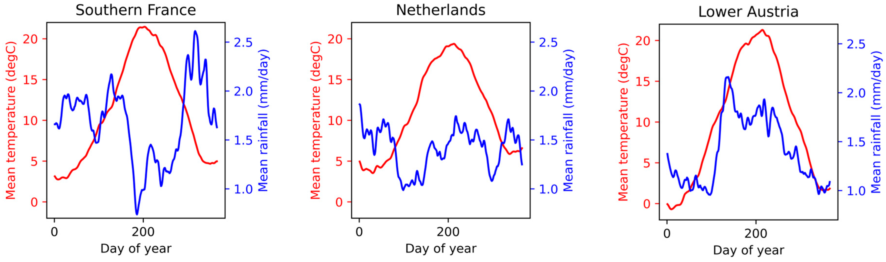
The Netherlands, Lower Austria, and southern France were chosen as study sites based on these criteria. The total area of the study covers an area of approximately 250,000 km2. Figure 1 shows the resulting three regions with the used crop parcels. Average temperatures and precipitation rates in these regions are displayed in Figure 2. While the mean annual temperatures are similar in the three regions, their seasonal behavior differs. The Netherlands is characterized by a maritime climate with winter temperatures above 0 °C and the lowest temperature in summer among the test sites. Lower Austria has the coldest winter with temperatures below 0 °C leading to frozen soil and warmer summer months than the Netherlands. Southern France, with its maritime climate, is very similar to Lower Austria but has slightly higher winter temperatures. Rainfall in the Netherlands is relatively high throughout the year. In Austria, most rainfall occurs during the summer months, whereas in southern France, these months are commonly the driest, and most rain falls in autumn.
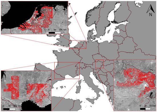
Figure 1.
Locations of the study sites in Europe. The field boundaries of the used parcels are outlined in red. (© EuroGeographics for the administrative boundaries).
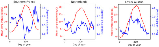
Figure 2.
Mean temperature and rainfall for the three study regions Netherlands, Lower Austria, and Southern France, derived from ERA5-Land [28].
2.2. Land Parcel Information System Data
Many countries collect information on field extents and planted crops in so-called Land Parcel Identification Systems (LPIS). For this study, freely available LPIS data for the study regions for all available years we obtained: for the Netherlands, this was the years 2016–2018, for Austria 2016–2019, and for France 2016–2017.
The selected crop types and number of sample parcels used in this study are summarized in Table 1. The selection of crops was based primarily on the cultivation in the individual countries. Crop types commonly grown in one country but not in the others (e.g., sunflowers in France) were excluded, as the used classification algorithms require a sufficiently large number of sample parcels per class for training. Moreover, the classes were chosen to cover crops with very similar phenology, such as wheat and barley, and crops with a very different plant structure, such as beet. In this way, the selected crops represent a large diversity of crop types.

Table 1.
Number of sample parcels per country and crop type accumulated over all years.
To create a harmonized dataset, several processing steps were applied to the LPIS data:
As the level of detail in the crop types in the LPIS data differs from country to country, classes needed to be merged to obtain a common classification key. Austria, for instance, provides information on the exact grassland type and the number of cuts per year, resulting in several different grassland classes. All these subclasses were merged into a single class grassland assuming that differences between sub-species can be neglected.
Since the Sentinel-1 time series derivation is computationally expensive, not all sample parcels in the LPIS data set for each crop type were used but only a subset of approximately at least 1500 sample parcels per year. For the season 2016 in France, this number could not be reached for SW with only 623 samples being available in the study site. The consequences for this on the experiments are outlined in Section 3.5.
A negative buffer of 10 m was applied to all field boundaries to ensure that the extracted Sentinel-1 pixels did not include land cover information from outside the field such as roads, forests, etc.
Small fields (<400 m2) were excluded from the reference database as these may not cover enough pixels to provide robust field statistics.
In this way, a total of 204,910 sample parcels were created. Some fields may have been selected in several consecutive years, so the total number of fields (parcels) can be smaller.
2.3. Sentinel-1
Sentinel-1 is a radar satellite mission operated by ESA that currently consists of two identical satellites with a C-band (5.4 GHz/5.6 cm) image sensor. The two satellites Sentinel-1A (launch April 2014) and Sentinel-1B (launch April 2016) each have a 12-day repeat cycle. As both satellites follow the same orbit plane with a 180° orbital phasing difference, the repeat cycle is six days or even less over Europe [30]. In this study, Ground Range Detected (GRD) high-resolution interferometric wide-swath (IW) data at a 10 m spatial sampling from the TU Wien Sentinel-1 data cube projected in the Equi7 Grid was used [31]. In IW mode, data is available for vertically polarized transmitted waves and vertically polarized received waves (VV) and for vertically transmitted but horizontally received (VH) polarized waves.
The pre-processing of Sentinel-1 IW GRD scenes was performed with the ESA SNAP (Sentinel Application Platform) software (version 6.0) and included the following steps [32]:
- Apply orbit file: the application of an orbit file is necessary to allow a precise orbit determination and the accurate satellite position and satellite velocity.
- Thermal noise removal: thermal noise removal is applied to remove atmospheric artifacts in the image.
- Radiometric calibration: radiometric calibration converts the backscatter intensity to a specified reference area. In this case, the backscatter coefficient sigma naught σ0.
- Range Doppler Terrain Correction: the Range Doppler Terrain Correction was performed with the SRTM 90 m DEM to reduce geometric impacts caused by the topography and to geocode the SAR scene.
2.4. Crop Dynamics in C-Band Radar
In contrast to the near-infrared band (~0.8–1.2 µm) of optical sensors, which is sensitive to the chlorophyll content of the vegetation canopy, the SAR backscatter signal reflects the geometric and dielectric properties of a surface. To simulate vegetation backscattering characteristics, models like the water-cloud model are commonly used [33]. They regard vegetation as a cloud of randomly oriented and distributed water droplets, which act as volume scatterers. Yet, the absolute backscatter from the vegetated layer not only includes the component backscattered from the vegetation but also from a second layer, the soil surface. The contribution of each layer for a constant incidence angle and wavelength mainly depends on the polarization. To monitor crop dynamics, the polarizations thus provide different information:
Cross-polarized VH waves are mainly sensitive to volume scattering that causes the depolarization of the emitted wave [34]. In terms of crop cultivation, VH thus reflects the plant water content, structure, and growth. This includes the process of stem extension, ears development, and cutting. Veloso et al. [9] outline that ground-stem-bounces and the rough surface also contribute to the signal. The degree of this contribution depends on the density of the vegetation layer. Satalino et al. [35] distinguish between crops with attenuated surface scattering such as wheat, and crops with mostly volume scattering such as rapeseed.
Co-polarized VV waves, in contrast, mainly reflect the soil contribution and ground-stem-bounces. Hence, VV is highly sensitive to the soil moisture (SM) content and the roughness of the soil [34]. As these properties do not reflect plant growth, they are usually not of interest for crop classification. However, previous studies have demonstrated the importance of VV polarized backscatter for discriminating tuber vegetables such as potatoes [8].
To reduce undesired SM influences, the cross-ratio (CR) of VH and VV polarization is commonly used for vegetation analysis. It is given by the equation CR = VH/VV and can also be expressed as decibels. Although more indices can be calculated from VH and VV backscatter, the CR has been tested extensively in recent studies [36]. Results from Khabbazan et al. [8] show that CR depicts the increase in biomass during the vegetative stages and the decrease in water content during senescence. Additionally, Vreugdenhil et al. [7] outline the suitability of the CR for monitoring crop dynamics. In another study, Vreugdenhil et al. [37] analyzed CR on a large scale over Europe and concluded that CR is highly correlated with vegetation optical depth over cropland. Thus, CR appears to be useful for monitoring vegetation dynamics over crop- and grassland.
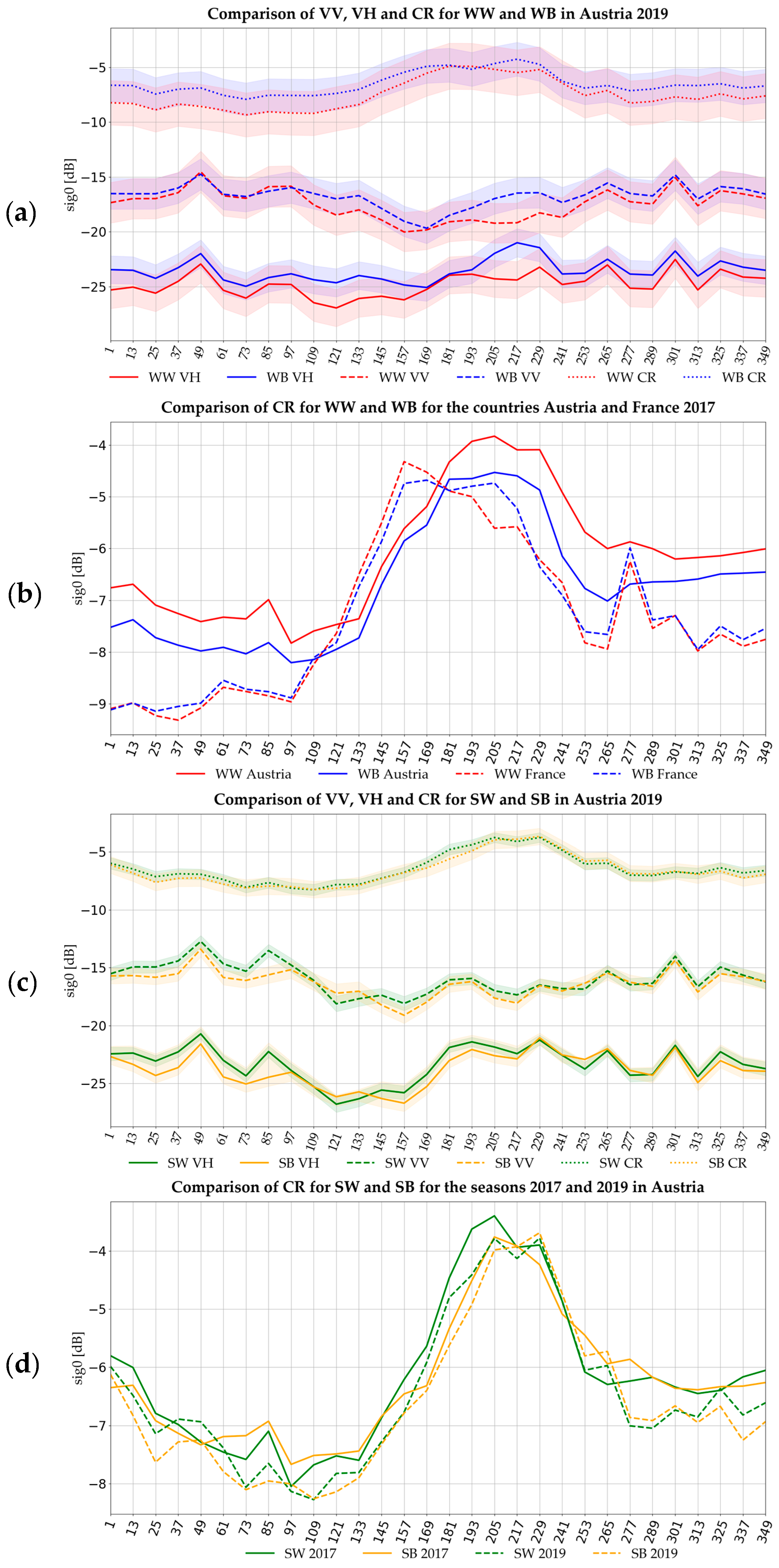
Figure 3 illustrates average time series for WW, WB, and SW, and SB for different polarizations, countries, and years. The timestamps are expressed as days since the beginning of the growing season (DOS), which is set here to November 1st of the year before the harvest. The first figure, Figure 3a, shows VH, VV polarization, and their CR for WW and WB in the season 2018/19 in Austria. In addition to the mean value, +/−1 standard deviations are added here (downscaled by the factor 0.2 to prevent a too large overlap between the polarizations). As the figure illustrates, the time series of both crops are very similar. Their main difference is the higher VH value in spring (around DOS 109–193) and the lower VV value in spring and summer (DOS 193–301) for WB. Consequently, the CR values for WB in this period are higher than those of WW. The latter also has a slightly higher variance compared to WB. For both crops, the variance in spring during the plant onset is higher compared to the end of the seasons. Figure 3b illustrates a comparison of WW and WB for Austria and France in the seasons 2016/17 for CR. Section 2.1 has stressed the different climate conditions in these countries. These changes are also reflected in the time series, as they significantly impact plant growth. Due to higher temperatures, the plant onset is earlier in France, which is reflected in the earlier increase of the WW and WB time series for France. In contrast, the CR value in Austria exceeds the one from France around DOS 172, presumably due to higher rainfall favoring the plant growth.
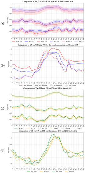
Figure 3.
Comparison of winter and summer wheat and barley time series in different polarizations, countries, and seasons. All figures show the mean over all available samples, Figure (a,c) show in addition +/− one-fifth standard deviation. The time axis shows the days since the beginning of the growing season (DOS).
Figure 3c, similar to Figure 3b, shows VV, VH, and CR time series in Austria 2018/19, but for SW and SB. For these crops, all time series are almost identical from DOS 253 to the end. Minor differences can be observed for SW with higher VV and VH values at the beginning of the season until DOS 138. The most characteristic difference is the earlier onset of SB in spring which is reflected in the earlier increase in VV polarization and the CR. Later, in early summer (around DOS 181), SW exceeds the development of SB and has higher VH and CR values. The figure also illustrates that the standard deviation of the SW and SB is significantly lower compared to WW and WB which might relate to the fact that the plant growth of winter crops is more influenced by the varying conditions in the winter month.
Finally, Figure 3d shows a comparison of the CR time series of the two seasons 2016/17 and 2018/19 in Austria. In both seasons SW has the earlier onset around DOS 155. However, presumably different weather conditions lead to different growing patterns in the summer month. Here, the peak of SB 2016/17 is much earlier than in 2018/19 and identical to the peak of SW 2018/19. At the same time, the decrease of SB 2018/19 (around DOS 229) is later than the one in 2016/17. It is also more similar to the SW than to the SB 2016/17 time series at this point.
These overlaps show that a distinction on a large spatiotemporal scale is challenging and stress the need to consider the entire time series for a class allocation, especially for crops with very similar plant development. Moreover, this discussion has shown that weather conditions (especially rainfall) impact time series indirectly by influencing crop growth and directly by changing the dielectric properties of the sensed area, and become increasingly important with increasing spatiotemporal scale. Therefore, meteorological data can be seen as an important input for crop classification.
2.5. Meteorological Data
To account for variable weather conditions, several atmospheric and land surface variables from ERA5-Land were extracted. ERA5-Land provides global climate reanalysis data with a grid spacing of approx. 9 km and 3-hourly timestamps [38]. Here, air temperature, rainfall, and soil water content of the upper two layers (0–7, 7–28 cm) were used. To allocate this data with the extracted Sentinel-1 time series, the data was resampled to 12 day interval time steps. Thereby, each given value corresponds to the average of the day of interest and the following 11 days. Based on these time steps, rolling averages over five consecutive timestamps were calculated for rainfall and soil water content. In doing so, not only the current weather conditions but also the conditions of the previous time steps are taken into account. In addition, growing degree days (GDD) were calculated from the daily temperature time series. GDD are a cumulative measure of days with expected plant growth based on air temperature [39]. These were calculated based on the equation
The base temperature Tbase is a constant value and describes the temperature which has to be exceeded to allow plant growth and was set to 5 °C based on average values found in the literature [40,41,42]. is the maximum temperature and is the minimum temperature recorded for every day.
2.6. Data Preparation
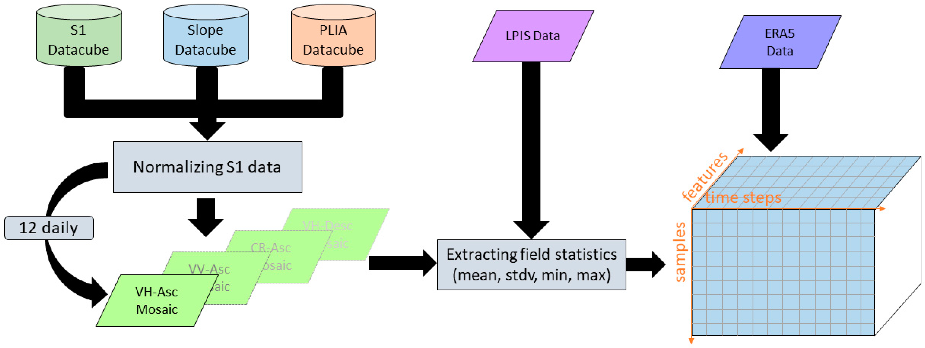
The crop classification in this study is based on time series per growing season, averaged on a field level. For every parcel, statistics were extracted for every polarization (VH and VV), CR, and ascending and descending orbit directions. These features are in the following referenced as SAR features. Per SAR feature several zonal statistics were calculated on field level: Mean, standard deviation, minimum value, and maximum value. Together with the four weather features, this sums up to a total of 28 features. For every time series, the start and end of every season were defined as the 1st of November and the end of October. This way, they cover the typical planting and harvesting dates of the included winter and summer crops. The detailed data preparation workflow is illustrated in Figure 4 and consisted of the following steps.
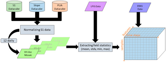
Figure 4.
Illustration of the data preparation workflow to extract time series on field level.
- Data cube initialization: Individual data cubes are initialized for Sentinel-1 data, projected local incidence angle (PLIA) files, and slope files. The data cubes include all available files for a defined spatial and temporal extent and required metadata for a filtering per orbit direction, polarization, and temporal information.
- Temporal data cube filtering: Starting from the 1st of November for every season, the data cubes were split into 12-day interval time steps to create a new data cube containing only files in the period. The 12-day interval time difference was chosen with respect to the 12-day repeat cycle of each Sentinel-1 satellite to guarantee a consistent amount of data for each time step. Due to the 180° orbit shift of Sentinel-1A and Sentinel-1B, six days would have also been possible. However, the advantage of averaging over 12 days is that high variability in SM is smoothed out, whereas changes in crop growth are expected to be slower. In addition, the processing time is decreased with a 12-day interval.
- Feature data cube: a separate data cube was created for every SAR feature, consisting of only the respective data (e.g., VV-ascending).
- S1 incidence angle normalization: All Sentinel-1 files were normalized to the same reference incidence angle of 38° degree, the mean incidence angle in IW mode. This was done to reduce the impact of the incidence angle on the backscatter signal caused by different acquisition geometries of the orbits. The normalization was performed using the formula:where the slope β describes the dependency of the backscatter on the incidence angle and is derived via linear regression of all available orbits per Equi7Grid tile. PLIA is defined as the local incidence angle projected into the range plane [43].
- 12-day interval mean images: Subsequently, the normalized Sentinel-1 files of every filtered data cube were used to create a “mean image” for the specific time step and all SAR features. This approach fulfills two purposes: temporal averaging reduces speckle effects, and short-term influences like SM on the backscatter signal are reduced.
- Extracting field stats: for every 12-day interval time step, zonal field statistics were calculated using the shapefiles from the LPIS data and written to a 3D array with a Field ID as the primary key.
- Adding ERA5-Land meteorological data: In a final step, the meteorological data was added to every field. As the ERA5-Land data has a coarse spatial resolution for each parcel, the data from the ERA5-land grid point closest to its centroid was used.
The outlined workflow was implemented in python using the “yeoda” Python package, which offers earth observation data cubes in python together with operations for their efficient filtering [44]. To ensure time-efficient processing, computing nodes from the Austrian supercomputer Vienna Scientific Cluster 3 were used to extract the time series. With this set-up, the total processing time for all countries and seasons amounted to 312 h on a single computing node.
3. Methods
Section 3 provides information on the two used algorithms LSTM network and RF and their training. In addition, it presents the used accuracy metrics and outlines the experimental scenarios.
3.1. LSTM Network
RNNs are Neural Networks for sequential data, where the input information is not flowing linearly but in feedback loops [45]. In this way, the previous output is used as an additional input next to the current input. However, the implemented feedback loops complicate the training process as the gradients are updated linearly and through a third temporal dimension. This is referred to as backpropagation through time. Thereby, the remaining error portions, especially for deep RNNs, can get so small that the weights in the front part of the network are barely adjusted. These circumstances make the training of RNNs very difficult and is referred to as the vanishing gradient problem. To overcome this disadvantage, LSTM networks use an additional state vector and multiple gates to control the flow of information throughout the network [46,47]. An illustration of a LSTM cell is presented in Figure 5. As illustrated, in addition to a current time step xt, two state vectors are forwarded as an input to the cell:
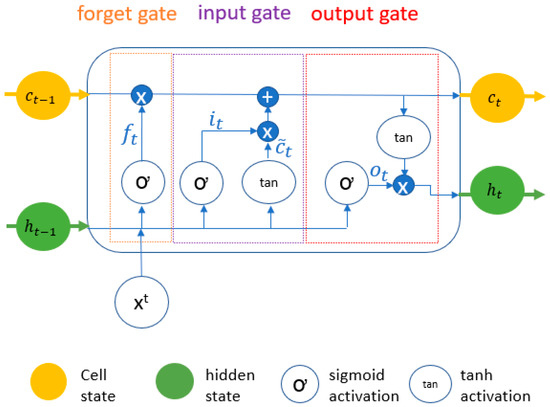
Figure 5.
Illustration of a LSTM cell.
- Hidden state: The hidden state ht has the same function as in a simple RNN. It carries information from a previous event to the next unit and is overwritten at every step.
- Cell state (memory cell): The cell state Ct is the main difference to a simple RNN. In combination with the gates, information can be written or removed from the cell state. This provides the LSTM network with the capability to store and load information of not only previous events but also of any point of the input sequence. This allows the network to learn long-term dependencies.
In addition to the two states, the LSTM network uses three gates to control the transmission of information to the state vectors by defining what is written or removed from the cell state or written to the hidden state:
- The input gate: the input gate It indicates the extent to which a new value flows into the cell.
- The output gate: the output gate Ot is the extent to which the value in the cell is used for the calculation of the next module in the chain.
- The forget gate: the forget gate Ft is the extent to which a value remains in the cell or is forgotten.
3.2. Random Forest
In this study, RF served as a baseline classifier, as it is widely used and proven to achieve high accuracies in a wide range of applications [48]. RF is a supervised learning approach that uses the bootstrap aggregating (short bagging) method that combines the predictions of several independent classification- or regression trees to determine the class allocation or prediction value. As in bagging, these predictions are made by randomly generated uncorrelated decision trees. These are built by choosing a random sample with replacement from the training data. RF expands this process by selecting a randomly selected subset of the data at the candidate splits during the bagging process. Each element is then assigned to a class based on the majority vote [49,50].
3.3. Model Training
The LSTM model in this study was implemented using the Python library “Keras” [51]. For all experiments, a bi-directional LSTM model with two layers and 321,032 trainable parameters was used. All models were trained from scratch using the Adam optimizer with a learning rate of 0.0007. The maximal number of training epochs was set to 120 with an early-stopping-monitor with a patience of eight. Early stopping ensures that the training process is stopped when the validation loss did not decrease over eight epochs. For all experiments, the dataset was split into 3/5 training, 1/5 validation, and 1/5 test data. The training and validation data was fed to the network with a batch size of 16 samples to fit and evaluate the model. After the training, model predictions were made for the test data to perform an unbiased accuracy assessment.
The RF classifier was implemented using the “sklearn” Python library [52]. To identify the best parameters for RF, a random search was carried out testing a wide range of values for the number of estimators, the max depth, and additional parameters. Using the best parameters from the random search, RF was then trained using 2/3 of the data and afterward tested using the remaining 1/3 of the data.
3.4. Accuracy Assessment
A classification report and a confusion matrix were calculated based on the model predictions for the test data. Precision, Recall, F1 score, and Overall Accuracy (OA) were chosen to measure the model performance as accuracy metrics to take both false positives and false negatives into account. Precision thereby is defined as the fraction of relevant instances among the retrieved instances and calculated using Equation (3). Recall (also known as Sensitivity) on the other hand is the fraction of relevant instances that were retrieved and can be derived using Formula (4). With known Precision and Recall values, the F1 score can be retrieved as their harmonic mean calculated via Equation (5) [53]. OA is calculated as the fraction of correctly classified samples among all samples.
3.5. Experimental Scenario Definition
In order to compare the performance of the LSTM and RF models, different scenarios with different degrees of spatiotemporal scale were defined. The scenario with the smallest spatiotemporal scale is one crop season in one country. In the second scenario, the temporal scale is increased to all seasons in one country. In the third, and most complex scenario, all seasons and all countries are used.
To ensure comparable results, we used the entire data set in all scenarios. As a consequence, scenarios 1 and 2 consists of several sub-scenarios which are listed in Table 2. For all scenarios, the model training and testing were carried out on the sub-scenario level. Thus, for the “single seasons/single country scenario”, a total of nine models were trained, for the “all seasons/single country” scenario three models, and for scenario 3 a single model. To ensure the highest possible accuracies can be achieved, hyperparameter tuning and parameter grid searches were performed on a sub-scenario level. The obtained confusion matrices of all sub-scenarios were afterward combined to a single matrix to retrieve, Precision, Recall, F1 scores, and OA for the entire scenario. For the sub-scenario France 2016, the sample size for SW was too small to properly train and evaluate the accuracy for this crop type. Therefore, this class was not considered for the accuracy metrics in this sub-scenario.
Table 2.
Overview of the three scenarios and their associated sub-scenarios used for the classification experiments in Section 4.
To increase the reliability of the results, all experiments were repeated at least five times, and the accuracy metrics were calculated as the average of those runs.
4. Results
The following section presents the results of this study. First, the classification results for the two algorithms are compared. Later they are related to the complexity of the experimental scenarios and their run time is evaluated. Finally, the importance of meteorological data is assessed.
4.1. Performance Comparison of the LSTM and RF Models
In a first step, the LSTM model was compared to the RF model for the in Section 3.5 introduced scenarios. Table 3 illustrates the obtained accuracies for the three scenarios. For scenario 1, both classifiers achieved a high accuracy of 87%. Accuracies for distinct crops are very similar except for SW and grassland. For the latter, the LSTM model achieved a five percentage point higher accuracy, whereas, for SW, RF shows a significantly higher accuracy with 79%.
Table 3.
Comparison of F1 scores and OA of the LSTM model with RF for different classification cases. Higher values for all scenarios and crop types are marked in bold.
Looking at the metrics for scenario 2, a significant decrease in accuracy for the RF model can be observed compared to scenario 1. In contrast, the overall accuracy remains at 87% for the LSTM model. For individual crop types, the most significant change can again be observed for wheat and barley. RF shows here a significant decrease for all cereals except for SB. In contrast, the LSTM model’s accuracies decreased slightly for the winter cereals but increased for the summer cereals. For potatoes, both classifiers show a significant decrease of around five percentage points.
For scenario 3, RF achieved an overall accuracy of 81%, the LSTM model again achieved an accuracy of 87%. In this case, accuracies differ between the models for a high number of crop types. Wheat and barley crops together with corn show higher accuracies in the LSTM model of around five percentage points. The highest differences occur for the class grassland with a ten percentage points higher value for the LSTM model. In contrast to RF, almost no differences between scenario 2 and scenario 3 are observed for the LSTM model.
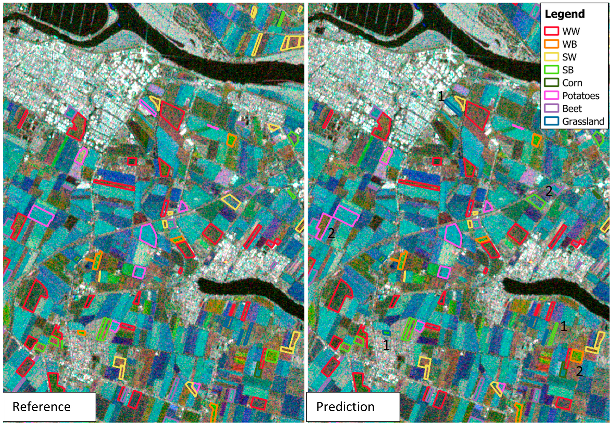
Figure 6 illustrates predicted crop classes for the sub-scenario Netherlands 2018 overlayed on a multi-temporal composite of three time steps. The misclassified fields indicate two major sources of classification errors: A lot of the misclassified fields a small or have narrow shapes (fields labeled with 1). Moreover, a lot of misclassifications occur among the winter and summer wheat and barley classes (fields labeled with 2).
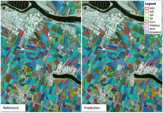
Figure 6.
Visualization of the reference LPIS data set (left) and predicted crop types (right) for a subset of the crop seasons 2018 in the Netherlands. The results are overlayed on a multitemporal composite of time steps at the beginning of May 2018 (red channel), mid of June 2018 (green channel), and mid of July 2018 (blue channel).
4.2. Relation of Classification Accuracy and Classification Complexity
The previous section indicates that with increasing scale, the LSTM network performs increasingly better than RF. To understand this effect, we refer to Section 1 and Section 2.4 that outlined that the variance of the crop time series increases with an increasing spatiotemporal scale. This leads to more complex class discrimination as the time series and feature spaces increasingly overlap, especially for crops with similar growth patterns. In this section, we quantify this increase in complexity and relate it to the performance differences of the LSTM and RF models.
As a basis for this quantification, we used a descriptor for classification complexity, the Fisher Discriminant Ratio F1 (FDR1) [54]. The FDR1 value describes how well the classes in each set-up can be discriminated by using linear discriminant analysis. A low value hereby indicates that there is at least one feature by which the classes can be separated from each other by a plane. In contrast, a high FDR1 value means that there is a (large) overlap between the classes and that a discrimination via a plane is not explicitly possible. Section 2.4 has shown that climate and weather conditions impact crop cultivation and the time series. As these factors highly vary between the investigated years and countries, we have a closer look at the sub-scenarios outlined in Table 4: As the complexity values for the investigated seasons in every country a very similar, we only included one season for each country.
Table 4.
Comparison of different classification cases with their corresponding Maximum Fisher’s Discriminant Ratio and the obtained OA for the LSTM model and Random Forest.
When comparing the accuracies with the FDR1 values, we can see a correlation for RF. In the single-season sub-scenarios for the Netherlands and France, the classifier performs well, in some cases even better than the LSTM model. For the scenarios with higher FDR1 values, however, the accuracies of the LSTM model exceed the corresponding accuracies of RF. The highest difference with 0.06 is observed for the scenario with the highest FDR1 value, the “all seasons/all countries scenario”.
4.3. Differences in Run Time
Table 4 also shows a comparison of the run-time of the two models. Both were run on a local machine with an Intel Core i7-6700k 4 core CPU with 4.00 GHz and 32 GB RAM. Despite having access to a GPU, we made the run time comparison on a local machine without GPU as most users do not have access to a GPU. Moreover, we assume RF to benefit from a GPU in a similar degree as the LSTM model well when using a RF library with GPU support such as “CuML”. Table 4 illustrates the expected differences in run time between the RF and the LSTM model. The latter shows much longer run times due to the need to adjust the parameters over several epochs. In addition to the sample size, a second factor that influences the run time is the early stopping monitor. In the countries Netherlands and France, which have a less complex feature space, early stopping monitor ends the training process earlier leading to a shorter run time. For RF, the run time mainly depends on the number of samples and increases almost linearly with the spatiotemporal scale.
4.4. Importance of Meteorological Data
Section 2.4. stressed that meteorological data can be considered as a valuable input for crop classification on a large spatiotemporal scale. In this section, we test the hypothesis, if model accuracies increase when the data from Section 2.5 is used as an additional input. To evaluate the hypothesis, we used the concept of permutation feature importance [55]. Hereby, one after the other, each input feature was randomized by shuffling the dataset among all samples. Afterward, both the LSTM and RF models were trained and tested as usual. The bigger the decrease of the accuracy, the higher the importance of the respective feature.
Table 5 illustrates the differences in accuracy when the meteorological data was not randomized. Green cells with positive values indicate an accuracy increase, whereas red cells with negative values represent a decrease in accuracy. The table shows that for the LSTM model, the meteorological data causes an increase in the OA and for the majority of the crops. Especially the winter and summer cereals benefit from the data. The biggest increase (0.06) in the F1 score is observed for grassland. RF on the other hand shows only an increase for winter and summer barley. Yet, the OA is not increasing as other crops show a decrease in accuracy. Computing the feature importance for the single weather features (GDD, rainfall, two layers of soil water content) shows that only GDD cause a measurable increase in the model performance (two percentage points), while other features increase the accuracy by less than one percentage point.
Table 5.
Differences with added meteorological data compared to when no meteorological data is used. An increase in accuracy is colored in green, decrease in red.
To determine if the obtained differences are statistically significant, we performed a paired t-test between the results from the experiments using meteorological data and no meteorological data for the LSTM model [56]. The calculated p-value is a measure identifying the significance of the difference between the compared cases. More precisely it gives the chance of observing the obtained differences even if the two compared means are identical. Based on this measurement, the differences for OA, grassland, and the summer and winter cereals are statistically significant (p-values ≤ 0.05).
5. Discussion
When comparing the performance for the individual crop types for scenario 3 in Table 3, the highest differences are observed for grassland, followed by barley, wheat, and corn. Potatoes and beets show the lowest differences in accuracy. As outlined in Section 2.4, barley and wheat have very similar growing seasons and profit from the LSTM model’s ability to learn long-term dependencies. This confirms findings from Ndikumana et al. [26] who observed advantages of LSTM networks for crops with similar growth patterns. Potatoes and beets have a high accuracy in general and the LSTM model shows no real improvement compared to RF. Beet has the latest harvest among the investigated crops and therefore a distinct growing pattern. Potatoes on the other hand have a discriminative peak in VV backscatter in early spring due to their cultivation in staggered rows. Therefore, these crops have unique features which explain the high accuracies.
The largest difference in accuracy between LSTM and RF is observed in grasslands. Bear in mind that the grassland class differs from the other classes in that it is not a cereal crop in the strict sense and, depending on the type of land use, can undergo no or several cuts per season. Therefore, there is a large variability in phenology between different grassland sample parcels. To understand the reason for this difference in accuracy between LSTM and RF, we calculated the Precision and Recall value for this class for the LSTM model and RF for the scenario 3. As Table 6 shows, the Recall value, in particular, differs significantly. This shows that in the case of the LSTM network significantly fewer samples were wrongly classified as grassland than in the case of RF. The reason for this most likely lies in the high variance of the class itself. Depending on the netting and cutting, the values of certain time periods fall into the feature space of other crop types. To separate the class reliably, it is thus necessary to consider several time steps and to learn their dependencies, which is one of the strengths of the LSTM model, as mentioned at the beginning.
Table 6.
Comparison of Precision, Recall, and F1 score for the class grassland with the LSTM model and RF for scenario 3.
The capability to learn long-term dependencies is also relevant with respect to the results in Section 4.2. Here it is important to remember that with increasing spatiotemporal scale, the variance in the time series increases as plant growth and harvest is shifted due to varying weather conditions. This leads to an increase in complexity and a decrease in the performance of RF. On the other hand, the model-specific characteristic to learn long-term dependencies become increasingly relevant here. This can be seen in the accuracies for the LSTM network, as they do not decrease significantly with increasing complexity.
As can be seen in Table 4, the main factor for increasing complexity is not an increase in spatial or temporal extent. Instead, the study region itself mainly defines the complexity: The classification tasks in the Netherlands show the lowest complexity values and for both classifiers the highest accuracies. France shows medium complexity and Austria the highest complexity values, only marginally lower than the values for the set-up with all countries and all seasons.
The reasons for country-specific differences in complexity are probably to be found in the different conditions there. As mentioned initially, frost has a tremendous influence on plant growth and therefore also on the time series of the crops [57]. Of the countries studied, Lower Austria has by far the highest number of frost days among the study sites with an average of 88 frost days (min. temperature below 0°) for all weather stations [58,59]. In addition, altitude has a significant impact on the number of frost days and thus on plant growth. Lower Austria also has the highest altitude and the highest difference in height among the test sites. Presumably, these circumstances lead to a high variance in cultivation and plant growth which is reflected in the SAR time series. Another factor to consider is the parcel size. Figure 6 has illustrated several of the misclassified fields are small or narrow. This corresponds to results from Orynbaikyzy et al. [16] who observed increasing classification accuracy with increasing field size, as the influence of speckle and adjacent classes on the field mean becomes smaller. With an average parcel size of 3.1 ha, fields in Lower Austria have the smallest field size among all study regions (Southern France 3.9 ha, Netherlands 5.6 ha).
The results from Section 4.4 allow us two conclusions: First, GDD are a valuable input that increases the LSTM model accuracy. Second, the LSTM model is capable to learn a certain dependency between meteorological data and other SAR features, as meteorological data alone does not allow a discrimination of different crop types. Based on Table 5 we can also conclude that foremost the class grassland benefits from the usage of meteorological data when considering multiple seasons and/or countries. Looking at the performance metrics Recall and Precision for the “all seasons/all countries” scenario with and without meteorological data in Table 7, we can see a comparable behavior as observed in the comparison between RF and the LSTM models for this class. Again, mainly the Recall values drop for the case that we do not use meteorological data. This leads to a similar conclusion as we have drawn with respect to Table 6: Without meteorological data, the class grassland is more difficult to discriminate from other classes as it has the highest in-class variance on average per time step. On the other hand, no notable drop in accuracy is obtained if we leave out meteorological data in the RF model. Thus, we conclude that the LSTM model in contrast to RF is capable of learning the relation between different input features and can extract high-level features, which results in higher accuracies for the LSTM model. In this way, we confirm findings from Schwalbert et al. [23] who observed similar behaviors for yield estimation.
Table 7.
Comparison of Precision, Recall, and F1 score for the class grassland when using meteorological data or no meteorological data as an input to the LSTM model for scenario 3.
6. Conclusions
This study found that LSTM networks show significant performance advantages over RF for a crop classification on a large spatiotemporal scale due to their capability to learn long-term dependencies and utilize meteorological data as an additional valuable input. However, this does not mean that a LSTM model is always the better choice. As the Free Lunch Theorem states, there is nothing like an overall best classifier as every advantage also comes with a disadvantage [60]. In the case of the LSTM model, we have to stress here the higher computation effort that comes along with requirements for GPUs or a longer computation time. Thus, for less complex classification tasks on a smaller spatiotemporal scale, a traditional ML classier can be preferable as both classifiers achieved comparable accuracies in our test scenarios. As an indicator of complexity, we used here the Fisher Discrimination Ratio. While this study focuses only on the architecture of LSTM due to its popularity, we assume our findings to be also valid for the very similar GRU model. The latter only differs in the gating function but has the same ability to learn long-term dependencies and extract high-level features. Moreover, we assume that our observations are not only valid for time series-based crop classification but also for similar time series applications. Future research will focus on the transferability of the model to regions with different climate conditions and the better utilization of meteorological data.
Author Contributions
Funding acquisition, M.V.; conceptualization, F.R., I.G.-P. and W.W.; methodology, F.R. and I.G.-P.; software, F.R.; validation, F.R. and I.G.-P.; formal analysis, F.R. and I.G.-P.; investigation, F.R. and I.G.-P.; resources, F.R. and I.G.-P.; data curation, F.R. and I.G.-P.; writing—original draft preparation, F.R.; writing—review and editing, F.R., I.G.-P., M.V. and W.W.; visualization, F.R. and I.G.-P.; supervision, W.W.; project administration, I.G.-P. and M.V. All authors have read and agreed to the published version of the manuscript.
Funding
This research was funded by the Austrian Space Application Program 15 (ASAP15) of the Austrian Research Promotion Agency (FFG) (FFG grant number 873721).
Institutional Review Board Statement
Not applicable.
Informed Consent Statement
Not applicable.
Data Availability Statement
The data presented in this study are available on request from the corresponding author.
Acknowledgments
The computational results presented have been achieved in part using the VSC. The authors acknowledge Open Access Funding by Vienna University of Technology Bibliothek.
Conflicts of Interest
The authors declare no conflict of interest.
Abbreviations
The following specific abbreviations are used in this manuscript:
| CR | Cross-ratio |
| DOS | Day of the Season |
| FDR1 | Fisher Discriminant Ratio F1 |
| GDD | Growing Degree Days |
| GRD | Ground Rage Detected |
| GRU | Gated Recurrent Unit |
| IW | Interferometric Wide Swath |
| LPIS | Land Parcel Information System |
| LSTM | Long Short-Term Memory |
| ML | Machine Learning |
| OA | Overall Accuracy |
| PLIA | Projected Local Incidence Angle |
| RF | Random Forest |
| RNN | Recurrent Neural Network |
| SAR | Synthetic Aperture Radar |
| SB | Summer Barley |
| SM | Soil Moisture |
| SW | Summer Wheat |
| VH | Vertical-Horizontal |
| VV | Vertical-Vertical |
| WB | Winter Barley |
| WW | Winter Wheat |
References
- FAO; IFAD; UNICEF; WFP; WHO. The State of Food Security and Nutrition in the World 2020; FAO: Rome, Italy; IFAD: Rome, Italy; UNICEF: Rome, Italy; WFP: Rome, Italy; WHO: Rome, Italy, 2020; ISBN 978-92-5-132901-6. [Google Scholar]
- United Nations, Department of Economic and Social Affairs. Population Division World Population Prospects 2019: Highlights 2019; United Nations, Department of Economic and Social Affairs: New York, NY, USA, 2019. [Google Scholar]
- World Meteorological Organization (WMO) State of the Climate in Africa 2019; World Meteorological Organization (WMO): Geneva, Switzerland, 2019.
- Benami, E.; Jin, Z.; Carter, M.R.; Ghosh, A.; Hijmans, R.J.; Hobbs, A.; Kenduiywo, B.; Lobell, D.B. Uniting Remote Sensing, Crop Modelling and Economics for Agricultural Risk Management. Nat. Rev. Earth Environ. 2021, 2, 140–159. [Google Scholar] [CrossRef]
- Navarro, A.; Rolim, J.; Miguel, I.; Catalão, J.; Silva, J.; Painho, M.; Vekerdy, Z. Crop Monitoring Based on SPOT-5 Take-5 and Sentinel-1A Data for the Estimation of Crop Water Requirements. Remote Sens. 2016, 8, 525. [Google Scholar] [CrossRef] [Green Version]
- Setiyono, T.; Quicho, E.; Gatti, L.; Campos-Taberner, M.; Busetto, L.; Collivignarelli, F.; García-Haro, F.; Boschetti, M.; Khan, N.; Holecz, F. Spatial Rice Yield Estimation Based on MODIS and Sentinel-1 SAR Data and ORYZA Crop Growth Model. Remote Sens. 2018, 10, 293. [Google Scholar] [CrossRef] [Green Version]
- Vreugdenhil, M.; Wagner, W.; Bauer-Marschallinger, B.; Pfeil, I.; Teubner, I.; Rüdiger, C.; Strauss, P. Sensitivity of Sentinel-1 Backscatter to Vegetation Dynamics: An Austrian Case Study. Remote Sens. 2018, 10, 1396. [Google Scholar] [CrossRef] [Green Version]
- Khabbazan, S.; Vermunt, P.; Steele-Dunne, S.; Ratering Arntz, L.; Marinetti, C.; van der Valk, D.; Iannini, L.; Molijn, R.; Westerdijk, K.; van der Sande, C. Crop Monitoring Using Sentinel-1 Data: A Case Study from The Netherlands. Remote Sens. 2019, 11, 1887. [Google Scholar] [CrossRef] [Green Version]
- Veloso, A.; Mermoz, S.; Bouvet, A.; Le Toan, T.; Planells, M.; Dejoux, J.-F.; Ceschia, E. Understanding the Temporal Behavior of Crops Using Sentinel-1 and Sentinel-2-like Data for Agricultural Applications. Remote Sens. Environ. 2017, 199, 415–426. [Google Scholar] [CrossRef]
- Chakhar, A.; Hernández-López, D.; Ballesteros, R.; Moreno, M.A. Improving the Accuracy of Multiple Algorithms for Crop Classification by Integrating Sentinel-1 Observations with Sentinel-2 Data. Remote Sens. 2021, 13, 243. [Google Scholar] [CrossRef]
- Xu, L.; Zhang, H.; Wang, C.; Zhang, B.; Liu, M. Crop Classification Based on Temporal Information Using Sentinel-1 SAR Time-Series Data. Remote Sens. 2019, 11, 53. [Google Scholar] [CrossRef] [Green Version]
- Tan, C.P.; Ewe, H.T.; Chuah, H.T. Agricultural Crop-Type Classification of Multi-Polarization SAR Images Using a Hybrid Entropy Decomposition and Support Vector Machine Technique. Int. J. Remote Sens. 2011, 32, 7057–7071. [Google Scholar] [CrossRef]
- Kenduiywo, B.K.; Bargiel, D.; Soergel, U. Crop-Type Mapping from a Sequence of Sentinel 1 Images. Int. J. Remote Sens. 2018, 39, 6383–6404. [Google Scholar] [CrossRef]
- Ustuner, M.; Sanli, F.B.; Abdikan, S.; Bilgin, G.; Goksel, C. A booster analysis of extreme gradient boosting for crop classification using PolSAR imagery. In Proceedings of the 2019 8th International Conference on Agro-Geoinformatics (Agro-Geoinformatics), Istanbul, Turkey, 16–19 July 2019; pp. 1–4. [Google Scholar]
- Nitze, I.; Schulthess, U.; Asche, H. Comparison of Machine Learning Algorithms Random Forest, Artificial Neural Network and Support Vector Machine to Maximum Likelihood for Supervised Crop Type Classification. In Proceedings of the 4th GEOBIA, Rio de Janeiro, Brazil, 7–9 May 2012; Volume 35. [Google Scholar]
- Orynbaikyzy, A.; Gessner, U.; Conrad, C. Crop Type Classification Using a Combination of Optical and Radar Remote Sensing Data: A Review. Int. J. Remote Sens. 2019, 40, 6553–6595. [Google Scholar] [CrossRef]
- Torbick, N.; Chowdhury, D.; Salas, W.; Qi, J. Monitoring Rice Agriculture across Myanmar Using Time Series Sentinel-1 Assisted by Landsat-8 and PALSAR-2. Remote Sens. 2017, 9, 119. [Google Scholar] [CrossRef] [Green Version]
- Shelestov, A.; Lavreniuk, M.; Vasiliev, V.; Shumilo, L.; Kolotii, A.; Yailymov, B.; Kussul, N.; Yailymova, H. Cloud Approach to Automated Crop Classification Using Sentinel-1 Imagery. IEEE Trans. Big Data 2020, 6, 572–582. [Google Scholar] [CrossRef]
- D’Andrimont, R.; Verhegghen, A.; Lemoine, G.; Kempeneers, P.; Meroni, M.; van der Velde, M. From Parcel to Continental Scale—A First European Crop Type Map Based on Sentinel-1 and LUCAS Copernicus in-Situ Observations. arXiv 2021, arXiv:210509261. [Google Scholar] [CrossRef]
- Zhong, L.; Hu, L.; Zhou, H. Deep Learning Based Multi-Temporal Crop Classification. Remote Sens. Environ. 2019, 221, 430–443. [Google Scholar] [CrossRef]
- Ebrahim, S.A.; Poshtan, J.; Jamali, S.M.; Ebrahim, N.A. Quantitative and Qualitative Analysis of Time-Series Classification Using Deep Learning. IEEE Access 2020, 8, 90202–90215. [Google Scholar] [CrossRef]
- Rusk, N. Deep Learning. Nat. Methods 2016, 13, 35. [Google Scholar] [CrossRef]
- Schwalbert, R.A.; Amado, T.; Corassa, G.; Pott, L.P.; Prasad, P.V.V.; Ciampitti, I.A. Satellite-Based Soybean Yield Forecast: Integrating Machine Learning and Weather Data for Improving Crop Yield Prediction in Southern Brazil. Agric. For. Meteorol. 2020, 284, 107886. [Google Scholar] [CrossRef]
- Jiang, H.; Hu, H.; Zhong, R.; Xu, J.; Xu, J.; Huang, J.; Wang, S.; Ying, Y.; Lin, T. A Deep Learning Approach to Conflating Heterogeneous Geospatial Data for Corn Yield Estimation: A Case Study of the US Corn Belt at the County Level. Glob. Chang. Biol. 2020, 26, 1754–1766. [Google Scholar] [CrossRef]
- Crisóstomo de Castro Filho, H.; Abílio de Carvalho Júnior, O.; Ferreira de Carvalho, O.L.; Pozzobon de Bem, P.; dos Santos de Moura, R.; Olino de Albuquerque, A.; Rosa Silva, C.; Guimarães Ferreira, P.H.; Fontes Guimarães, R.; Trancoso Gomes, R.A. Rice Crop Detection Using LSTM, Bi-LSTM, and Machine Learning Models from Sentinel-1 Time Series. Remote Sens. 2020, 12, 2655. [Google Scholar] [CrossRef]
- Ndikumana, E.; Ho Tong Minh, D.; Baghdadi, N.; Courault, D.; Hossard, L. Deep Recurrent Neural Network for Agricultural Classification Using Multitemporal SAR Sentinel-1 for Camargue, France. Remote Sens. 2018, 10, 1217. [Google Scholar] [CrossRef] [Green Version]
- Zhao, H.; Chen, Z.; Jiang, H.; Jing, W.; Sun, L.; Feng, M. Evaluation of Three Deep Learning Models for Early Crop Classification Using Sentinel-1A Imagery Time Series—A Case Study in Zhanjiang, China. Remote Sens. 2019, 11, 2673. [Google Scholar] [CrossRef] [Green Version]
- Pelletier, C.; Webb, G.I.; Petitjean, F. Deep learning for the classification of sentinel-2 image time series. In Proceedings of the IGARSS 2019—2019 IEEE International Geoscience and Remote Sensing Symposium, Yokohama, Japan, 28 July–2 August 2019; pp. 461–464. [Google Scholar]
- He, T.; Xie, C.; Liu, Q.; Guan, S.; Liu, G. Evaluation and Comparison of Random Forest and A-LSTM Networks for Large-Scale Winter Wheat Identification. Remote Sens. 2019, 11, 1665. [Google Scholar] [CrossRef] [Green Version]
- Torres, R.; Snoeij, P.; Geudtner, D.; Bibby, D.; Davidson, M.; Attema, E.; Potin, P.; Rommen, B.; Floury, N.; Brown, M.; et al. GMES Sentinel-1 Mission. Remote Sens. Environ. 2012, 120, 9–24. [Google Scholar] [CrossRef]
- Bauer-Marschallinger, B.; Sabel, D.; Wagner, W. Optimisation of Global Grids for High-Resolution Remote Sensing Data. Comput. Geosci. 2014, 72, 84–93. [Google Scholar] [CrossRef]
- SkyWatch; German Aerospace Center (DLR); Brockmann Consult; OceanDataLab. Sentinel-1 Toolbox. 2021. Available online: https://step.esa.int/main/toolboxes/sentinel-1-toolbox/ (accessed on 29 January 2021).
- Attema, E.P.W.; Ulaby, F.T. Vegetation Modeled as a Water Cloud. Radio Sci. 1978, 13, 357–364. [Google Scholar] [CrossRef]
- Woodhouse, I.H. Introduction to Microwave Remote Sensing; Taylor & Francis: Boca Raton, FL, USA, 2006; ISBN 978-0-415-27123-3. [Google Scholar]
- Satalino, G.; Balenzano, A.; Mattia, F.; Davidson, M.W.J. C-Band SAR Data for Mapping Crops Dominated by Surface or Volume Scattering. IEEE Geosci. Remote Sens. Lett. 2014, 11, 384–388. [Google Scholar] [CrossRef]
- Holtgrave, A.-K.; Röder, N.; Ackermann, A.; Erasmi, S.; Kleinschmit, B. Comparing Sentinel-1 and -2 Data and Indices for Agricultural Land Use Monitoring. Remote Sens. 2020, 12, 2919. [Google Scholar] [CrossRef]
- Vreugdenhil, M.; Navacchi, C.; Bauer-Marschallinger, B.; Hahn, S.; Steele-Dunne, S.; Pfeil, I.; Dorigo, W.; Wagner, W. Sentinel-1 Cross Ratio and Vegetation Optical Depth: A Comparison over Europe. Remote Sens. 2020, 12, 3404. [Google Scholar] [CrossRef]
- Copernicus Climate Change Service ERA5-Land Hourly Data from 2001 to Present 2019. Available online: https://cds.climate.copernicus.eu/doi/10.24381/cds.e2161bac (accessed on 24 May 2021).
- McMaster, G.S.; Wilhelm, W.W. Growing Degree-Days: One Equation, Two Interpretations. Agric. For. Meteorol. 1997, 87, 291–300. [Google Scholar] [CrossRef] [Green Version]
- Skaggs, K.E.; Irmak, S. Long-Term Trends in Air Temperature Distribution and Extremes, Growing Degree-Days, and Spring and Fall Frosts for Climate Impact Assessments on Agricultural Practices in Nebraska. J. Appl. Meteorol. Climatol. 2012, 51, 2060–2073. [Google Scholar] [CrossRef] [Green Version]
- Skakun, S.; Franch, B.; Vermote, E.; Roger, J.-C.; Becker-Reshef, I.; Justice, C.; Kussul, N. Early Season Large-Area Winter Crop Mapping Using MODIS NDVI Data, Growing Degree Days Information and a Gaussian Mixture Model. Remote Sens. Environ. 2017, 195, 244–258. [Google Scholar] [CrossRef]
- Wypych, A.; Sulikowska, A.; Ustrnul, Z.; Czekierda, D. Variability of Growing Degree Days in Poland in Response to Ongoing Climate Changes in Europe. Int. J. Biometeorol. 2017, 61, 49–59. [Google Scholar] [CrossRef] [Green Version]
- Bauer-Marschallinger, B.; Cao, S.; Navacchi, C.; Freeman, V.; Reuß, F.; Geudtner, D.; Rommen, B.; Vega, F.C.; Snoeij, P.; Attema, E.; et al. The Normalised Sentinel-1 Global Backscatter Model, Mapping Earth’s Land Surface with C-Band Microwaves. Sci. Data 2021, 8, 277. [Google Scholar] [CrossRef] [PubMed]
- TU Wien GEO Department. yeoda–GitHub. Available online: https://github.com/TUW-GEO/yeoda (accessed on 3 April 2021).
- Rumelhart, D.E.; Smolensky, P.; McClelland, J.L.; Hinton, G.E. Schemata and sequential thought processes in PDP models. In Parallel Distributed Processing: Explorations in the Microstructure, Vol. 2: Psychological and Biological Models; MIT Press: Cambridge, MA, USA, 1986; pp. 7–57. ISBN 0-262-63110-5. [Google Scholar]
- Hochreiter, S.; Schmidhuber, J. LSTM can solve hard long time lag problems. In Proceedings of the 9th International Conference on Neural Information Processing Systems, Denver, CO, USA, 3–5 December 1996; MIT Press: Cambridge, MA, USA, 1996; pp. 473–479. [Google Scholar]
- Hochreiter, S.; Schmidhuber, J. Long Short-Term Memory. Neural Comput. 1997, 9, 1735–1780. [Google Scholar] [CrossRef]
- Fernández-Delgado, M.; Cernadas, E.; Barro, S.; Amorim, D. Do We Need Hundreds of Classifiers to Solve Real World Classification Problems? J. Mach. Learn. Res. 2014, 15, 3133–3181. [Google Scholar]
- Breiman, L. Bagging Predictors. Mach. Learn. 1996, 24, 123–140. [Google Scholar] [CrossRef] [Green Version]
- Breiman, L. Random Forests. Mach. Learn. 2001, 45, 5–32. [Google Scholar] [CrossRef] [Green Version]
- Chollet, F. Keras—GitHub. Available online: https://github.com/keras-team/keras (accessed on 2 February 2021).
- Pedregosa, F.; Varoquaux, G.; Gramfort, A.; Michel, V.; Thirion, B.; Grisel, O.; Blondel, M.; Prettenhofer, P.; Weiss, R.; Dubourg, V.; et al. Scikit-Learn: Machine Learning in Python. J. Mach. Learn. Res. 2011, 12, 2825–2830. [Google Scholar]
- Zeugmann, T.; Poupart, P.; Kennedy, J.; Jin, X.; Han, J.; Saitta, L.; Sebag, M.; Peters, J.; Bagnell, J.A.; Daelemans, W.; et al. Precision and recall. In Encyclopedia of Machine Learning; Sammut, C., Webb, G.I., Eds.; Springer US: Boston, MA, USA, 2011; p. 781. ISBN 978-0-387-30768-8. [Google Scholar]
- Lorena, A.C.; Garcia, L.P.; Lehmann, J.; Souto, M.C.; Ho, T.K. How Complex Is Your Classification Problem? A Survey on Measuring Classification Complexity. ACM Comput. Surv. CSUR 2019, 52, 1–34. [Google Scholar] [CrossRef] [Green Version]
- Fisher, A.; Rudin, C.; Dominici, F. All Models Are Wrong, but Many Are Useful: Learning a Variable’s Importance by Studying an Entire Class of Prediction Models Simultaneously. arXiv 2019, arXiv:180101489. [Google Scholar]
- Student The Probable Error of a Mean. Biometrika 1908, 6, 1. [CrossRef]
- Wang, S.; Chen, J.; Rao, Y.; Liu, L.; Wang, W.; Dong, Q. Response of Winter Wheat to Spring Frost from a Remote Sensing Perspective: Damage Estimation and Influential Factors. ISPRS J. Photogramm. Remote Sens. 2020, 168, 221–235. [Google Scholar] [CrossRef]
- Amt der Niederösterr, Landesregierung, Abt, Raumordnung und Regionalpolitik, Sachgebiet Statistik. Statistisches Handbuch des Landes Niederösterreich. 41.2017; NÖ Schriften; Amt der Niederösterr, Landesregierung, Abt, Raumordnung und Regionalpolitik, Sachgebiet Statistik: St. Pölten, Austria, 2017; ISBN 978-3-85006-215-2. [Google Scholar]
- CBS; PBL; RIVM; WUR. Meteorologische Gegevens, 1990–2020. Available online: https://www.clo.nl/indicatoren/nl000423 (accessed on 12 September 2021).
- Wolpert, D.H.; Macready, W.G. No Free Lunch Theorems for Optimization. IEEE Trans. Evol. Comput. 1997, 1, 67–82. [Google Scholar] [CrossRef] [Green Version]


Publisher’s Note: MDPI stays neutral with regard to jurisdictional claims in published maps and institutional affiliations. |
© 2021 by the authors. Licensee MDPI, Basel, Switzerland. This article is an open access article distributed under the terms and conditions of the Creative Commons Attribution (CC BY) license (https://creativecommons.org/licenses/by/4.0/).