Article

Improvement of the Soil Moisture Retrieval Procedure Based on the Integration of UAV Photogrammetry and Satellite Remote Sensing Information

by
Amal Chakhar
*,
David Hernández-López
,
Rocío Ballesteros
and
Miguel A. Moreno
Institute of Regional Development, University of Castilla-La Mancha, 02071 Albacete, Spain
*
Author to whom correspondence should be addressed.
Remote Sens. 2021, 13(24), 4968; https://doi.org/10.3390/rs13244968
Submission received: 27 October 2021 / Revised: 30 November 2021 / Accepted: 1 December 2021 / Published: 7 December 2021
(This article belongs to the Special Issue Satellite Soil Moisture Validation and Applications)

Abstract

:
In countries characterized by arid and semi-arid climates, a precise determination of soil moisture conditions on the field scale is critically important, especially in the first crop growth stages, to schedule irrigation and to avoid wasting water. The objective of this study was to apply the operative methodology that allowed surface soil moisture (SSM) content in a semi-arid environment to be estimated. SSM retrieval was carried out by combining two scattering models (IEM and WCM), supplied by backscattering coefficients at the VV polarization obtained from the C-band Synthetic Aperture Radar (SAR), a vegetation descriptor NDVI obtained from the optical sensor, among other essential parameters. The inversion of these models was performed by Neural Networks (NN). The combined models were calibrated by the Sentinel 1 and Sentinel 2 data collected on bare soil, and in cereal, pea and onion crop fields. To retrieve SSM, these scattering models need accurate measurements of the roughness surface parameters, standard deviation of the surface height (hrms) and correlation length (L). This work used a photogrammetric acquisition system carried on Unmanned Aerial Vehicles (UAV) to reconstruct digital surface models (DSM), which allowed these soil roughness parameters to be acquired in a large portion of the studied fields. The obtained results showed that the applied improved methodology effectively estimated SSM on bare and cultivated soils in the principal early growth stages. The bare soil experimentation yielded an R2 = 0.74 between the estimated and observed SSMs. For the cereal field, the relation between the estimated and measured SSMs yielded R2 = 0.71. In the experimental pea fields, the relation between the estimated and measured SSMs revealed R2 = 0.72 and 0.78, respectively, for peas 1 and peas 2. For the onion experimentation, the highest R2 equaled 0.5 in the principal growth stage (leaf development), but the crop R2 drastically decreased to 0.08 in the completed growth phase. The acquired results showed that the applied improved methodology proves to be an effective tool for estimating the SSM on bare and cultivated soils in the principal early growth stages.

Graphical Abstract

1. Introduction

Soil surface moisture (SSM) is the main factor of water and heat fluxes in the soil-plant-atmosphere continuum that plays a key role in determining crop water supply, which is crucial for the vegetation health [1]. Many applications [2], such as agricultural, environmental and socio-economic ones, need precise determinations of SSM dynamics.
The sensitivity of the radar backscattering coefficient, σ 0 , to SSM leads to significant interest in exploiting radar remote sensing data to retrieve SSM information. Nevertheless, radar measurements are associated with moisture and roughness characteristics of soil surface [3]. Many electromagnetic models, such as the Kirchoff Approximations [4], the small perturbation model (SPM) [5] and the integral equation model (IEM) [6], have been created to study backscattering and to simulate radar backscattering coefficient, σ 0 , data on bare soils as a function of roughness and moisture. As the Kirchoff and SPM models are applicable to limited conditions (particularly roughness conditions) [3], many attempts have been made to extend their validity domain, which has resulted in the development of the IEM. This developed model (IEM) combines Kirchhoff and SPM models to create a method that can be used for a more extensive range of roughness conditions and applied to any location [7]. The challenge of these soil scattering models’ calibration lies in the soil surface description [8]. Thus, the hardest point of developing soil moisture retrieval models is to determine the surface roughness parameters: the standard deviation of the surface height variation (hrms) and the correlation length (L). These parameters significantly affect the relations between radar backscatter and soil moisture [9].
Quite a high degree of uncertainty exists in the parameterization of soil surface roughness, which leads to major soil moisture retrieval errors [10]. Baghdadi et al. [11] reviewed the difficulties of accurately measuring those parameters. One of them is the difficulty to measure the correlation length, L, because of the substantial instability of agricultural soil. According to several studies, the backscattering coefficient varies considerably depending on the correlation function shape [12]. L is calculated from the correlation function and is always extremely variable, even on plots with homogenous soil [13]. This variability can lead to significant errors in the simulated radar signal [11]. It is reported in [14] that when the IEM fails to provide good results when applied to natural soil, this can be attributed to an inadequate description of this surface rather than a malfunction of the model.
As reported in [15], there are several methods for soil roughness assessment techniques that involve different soil height sampling techniques and data analysis strategies. Classic roughness sampling techniques are pin and mesh-board profilers, which collect individual soil roughness profiles with a length ranging from 0.5 to 4 m, and a regular sampling distance ranging from 5 to 10 mm along the profile direction [16]. Laser profilers are a non-destructive alternative. An example of this category is a laser profiler constructed by the CESBIO (the Center of the study of the Biosphere from Space, Toulouse, France) and the ESA (European Space Agency, Paris, France). This profiler can regularly sample heights at every 5 mm and collect up to 25 m long profiles [9]. In the bibliography, the description of soil surface roughness patterns includes soil surface roughness measurements taken by photogrammetric acquisition systems [3,17,18], and recently by terrestrial laser scanners (TLS) [15].
Roughness measurements are usually taken with a pin profiler [19,20,21,22,23,24]. In most cases, this tool is restrained to a one-dimension profile that can hardly lead to a 3D soil structure characterization. However, to obtain precise statistical parameters, it is crucial to consider many profiles for each studied field [17]. Consequently, new technologies based on photogrammetric techniques can produce a 3D model of any surface from digital photographs to make more precise estimations of roughness indices. The studies achieved in [14,18] reported an efficient general methodology of the photogrammetric process to acquire an estimation of roughness indices. Thus, terrestrial laser scanners (TLS) were used. The study performed in [15] demonstrated that TLS are an effective tool for modeling soil roughness on low scales. On the other hand, given the number of required stand points, the application of the TLS tool to large areas is not practical. This is why unmanned aerial vehicles’ (UAV) acquisition, followed by the photogrammetric process of the acquired images, can provide a better solution [19]. Additionally, the authors of [20] investigated the potential of the C-band at VV polarization obtained by Sentinel 1 for estimating the soil roughness parameter hrms on bare soil. Nevertheless, they found that the obtained accuracy of the soil roughness estimates did not meet the requirement of the operational users of soil roughness products.
The authors of [10,21] stated that it is complicated to measure the required roughness parameters, particularly L. Therefore, given the difficulty to determine soil roughness parameters and, at the same time, their primordial necessity in soil moisture retrieval models, some studies suggest methodologies that avoid the direct measurement of these parameters. For example, the authors of [22] did not measure roughness parameters, but only collected information about the roughness class for each reference plot during the field campaigns according to three classes: smooth, medium and rough. In another study [23], the authors suggested a semi-empirical calibration of IEM backscattering to reduce the incompatibilities between simulated and measured backscattering values. This calibration consists in substituting the measured L in the field by a fitting parameter called Lopt, which depends on hrms, incidence angle, polarization and radar wavelength.
According to the bibliographic review, practically all the works have retrieved SSM using backscatter models employing in situ measurements limited to small areas to estimate soil roughness parameters or indirect methods. As photogrammetric acquisition systems have already been used to describe soil surface roughness patterns, their combination with remote sensing techniques, such as UAV, can cover larger areas [24]. The present study aimed to apply an operational methodology that has been previously tested for soil moisture estimates to agricultural fields [22]. To further improve these results, roughness parameters were measured by a photogrammetric acquisition system carried on a UAV to reconstruct digital surface models (DSM). The acquisition of DSM allowed the procurement of these parameters over a large portion of our experimental agricultural fields. Our improved methodology started by accurately measuring the roughness parameters of these fields. This step required meticulous fieldwork (preparing the flight and equipment, choice of flight period to coincide with plowing dates, among others), as well as a photogrammetry process to obtain DSM and an efficient approach to acquire both L and hrms. After determining soil roughness parameters, their implications on the σ 0 estimation were studied. To retrieve soil moisture, backscattering models were applied (the IEM and the Water Cloud Model (WCM)). Then, the main study objective was to retrieve SSM using Sentinel 1 and 2 data and to follow an operative approach, improved by integrating the accurate roughness parameters measured by photogrammetric processes.

2. Materials and Methods

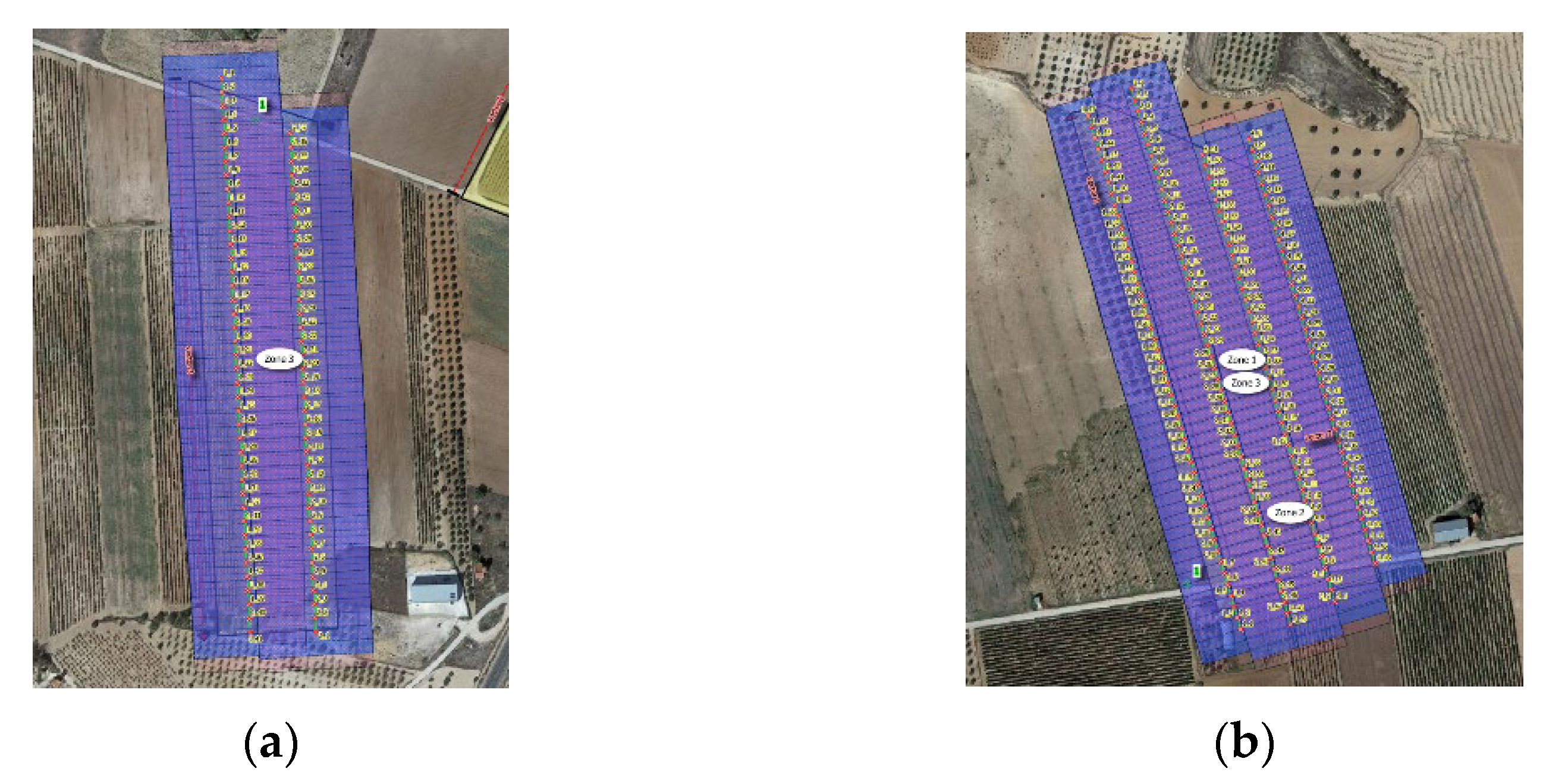
2.1. Test Site 1: Bare Soil Plot

Research was carried out at two experimental sites (Figure 1): the first on a small bare soil plot located at the experimental farm of the University of Castilla-La Mancha in Albacete province, Spain (27.5 m wide, 32 m long). Its soil has a silty-clay texture (21.2% clay, 52.3% sand and 26.5% silt). The soil depth of the soil particle analysis was between 5 and 10 cm deep. The soil roughness parameters were taken when soil had been recently plowed.

2.2. Test Site 2: Open Field Crops

The second test site was an irrigable area in Tarazona de La Mancha, Spain (Figure 1). Experimentation was carried out on four different crop fields: one cereal plot with an area equal to 2 ha, two pea plots (peas 1 and peas 2) covering 2.2 and 2.28 ha, respectively, and one onion plot whose area covered 2.8 ha (Figure 1). Tarazona de la Mancha (39.7 N–38.6 N and 2.53 W–0.9 W) is located in the Castilla-La Mancha region of Spain. Its climate is semi-arid with annual precipitation below 350 mm. The spatial distribution of the reference evapotranspiration (ETo) varies from 1151 mm year-1 to more than 1300 mm year-1 in the northwest and southeast portions of the aquifer, respectively. The average temperatures range from 3.97 °C in January, the coldest month, to 24.37° in July, the warmest month. The dominant crops are wheat, barley, vine, alfalfa, onion, garlic, poppy and legumes. The soil analysis results for each plot show that soil has a silty-clay texture (Table 1).

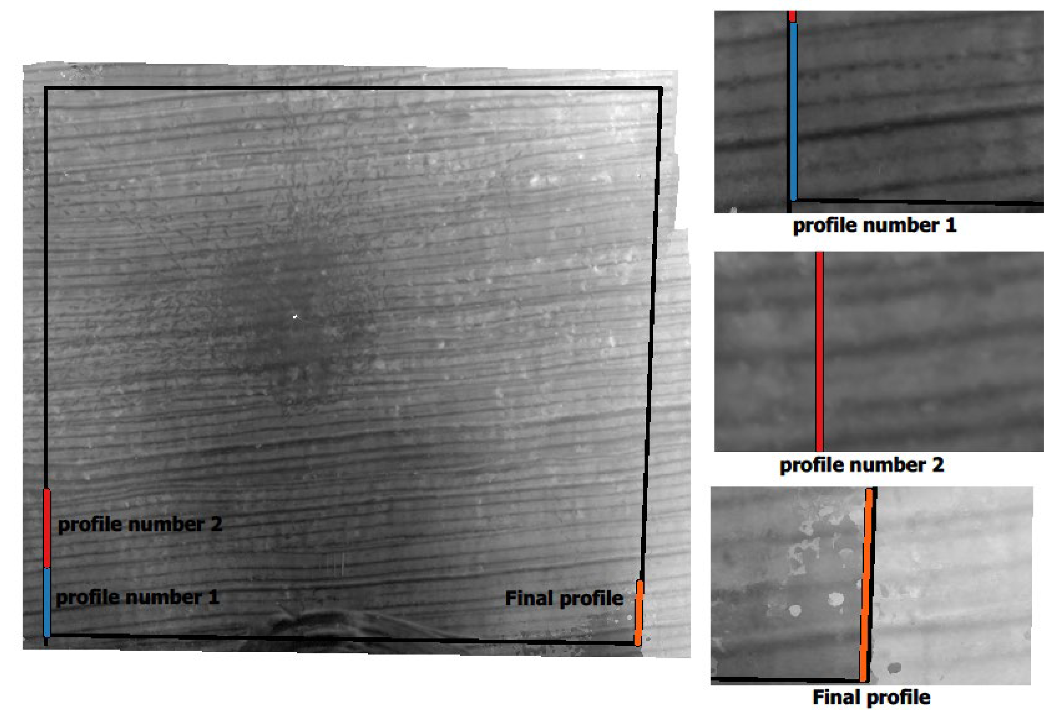
2.3. Soil Roughness Characterization and the Photogrammetry Process

For modeling objectives, a given surface is defined statistically by two variables, determined from the surface height profiles: L and hrms [25]. Information was obtained using a conventional SONY ILCE-5100 RGB digital camera (Sony Corporation, Tokyo, Japan) mounted on a drone to determine soil surface roughness. Flights were planned at 20 m above the ground level, with a 40% side overlap and an 80% front overlap, which resulted in a ground sample distance (GSD) of 4 mm. For all the flight events (Table 2), illumination was optimal with no clouds.
In this study, an Icom3D–Carabo S3 drone was utilized. It is a vertical take-off and landing (VTOL) quadcopter aircraft with a high payload/MTOW rate (up to 1 kg of payload in 2.6 kg of MTOW). It offers multiple customizable payload options with a compact design. UAV can follow a pre-programmed flight plan to determine the route and camera shooting events (Figure 2). In addition, six ground control points (GCP), measured with a GNSS-RTK device (accuracy over 0.02 m in altitude), were placed for each flight to geo-reference the final geomatic product and to perform camera calibration.
DSM were obtained using the structure from motion (SfM) software, the Agisoft Metashape Professional version 1.6.1 software (Agisoft LLC, St. Petersburg, Russia), to determine soil surface roughness parameters. The photogrammetric process steps are summarized below.
The first step extracts features from each single image that can be matched to their corresponding feature in other images, followed by an approximate alignment of the images with a sufficient number of features.
The second step determines the camera’s intrinsic (focal length, principal point and lens distortion) and extrinsic (projection center location and the six exterior orientation parameters defining the image) orientation parameters by determining optimal camera positions, and later ameliorating their positions with a bundle-adjustment algorithm. A sparse point cloud with the location and position of every supplied image is the result of following the first two steps.
The third step exploits the previously determined intrinsic and extrinsic camera locations, a dense Multi-View Stereo (MVS) reconstruction and every pixel of the provided images to produce a dense point cloud.
The resulting dense point cloud is generated in an arbitrary coordinate system. However, Agisoft Photoscancan transforms the model into the absolute coordinate system provided by a minimum of three ground control points (GCP) or camera coordinates that have been recorded. This is why GCP are introduced in this step to enable the processing software to know the real-world coordinates of a number of visibly identifiable locations on the imagery [26].

2.4. Acquisition Methodology Considering the Spatial Variability of Soil Roughness

One of the main constraints for determining roughness parameters is that they show little or no spatial dependency [27]. Alternatively, the surface measurements and L taken at one position often do not, or only poorly, represent their surrounding area, which makes this information physically meaningless. Therefore, we propose following a methodology based on obtaining massive 2 m long profiles to calculate these surface roughness indices, and to then perform a statistical analysis with the set of indices calculated for each profile. For this purpose, the DSM of the experimental field was converted into an XYZ matrix. The surface roughness indices were estimated using virtual profiles of a 2 m length, which moved all over the DSM from the lower left corner to the lower right corner (Figure 3), and always maintained the azimuth direction perpendicular to the row. Next, and as in [27], the hrms values were obtained as the arithmetic mean of all the individual hrms values. The average L values were derived from the average autocorrelation function (ACF), calculated using the ACFs of the individual profiles.
In agricultural fields, soil roughness is affected by tillage characteristics [9,28]. According to [18], roughness should be measured in perpendicular and parallel directions to seedbed rows because the soil surface can be considered anisotropic [29]. However, the authors of [30,31] revealed a significant impact on the backscattered signal scale from the periodical roughness component. Hence, we focused only on the perpendicular measurements to row directions, which are mainly influenced by the periodical component. The authors of [18] found that the roughness measurement taken perpendicularly to row directions indicated two significant issues: first, the studied surface showed a clear trend that had to be corrected; second, the perpendicular profiles to the row direction showed a two-scale process that had to be separately quantified. Therefore, in this work, we applied the two major corrections proposed in [27]: detrending and decomposing data into two scales.
The tillage induced a roughness deviation compared to the curved reference surface, described by a single-scale process [21]. Therefore, to parameterize these single-scale roughness deviations, it was necessary to filter out the curved reference surface. The authors of [10,21] stated that different methodologies can be applied, such as detrending using piecewise linear regressions, applying a high-pass filter or a moving average filter and detrending with a higher-order polynomial. However, removing the overall first-order trend is generally sufficient [10], although such a detrending technique may not be sufficient for long profiles because roughness parameters increase with growing transect length (to reveal a multiscale effect). This assumption is only valid when short profiles are measured [21]. Based on the literature review and the characteristics of the analyzed plots, only the removal of the first-order trend was applied. Indeed, detrending was performed by subtracting a trend surface ( Z m o d ) from the original surface (Z). The detrended surface ( Z r e s ) was defined as:
Z r e s = Z Z m o d
Z m o d   ~   m   X + b
where m and b represent the regression coefficients of slope and intercept, while X is the x-coordinate of the sampled profile retrieved from DSM (this operation was repeated for all the n profiles extracted from the DSM).

2.5. Roughness Parameters

The standard deviation of the hrms of the discrete one-dimensional case was:
hrms = i = 1 n ( Z i Z ¯ ) 2 n 1
where n is the number of samples and Zi is the altitude of the point at position xi.
Z ¯   =   1 n i = 1 n Z i  
The ACF provides some information about the distribution of hills and valleys across the surface [32] because it represents the correlation of paired-sample measurements according to the distance between samples [14], defined as:
C ^ ( h ) = 1 N ( h ) i = 1 N ( h ) Z ( x i + h ) Z ( x i )
where N(h) is the number of pairs of points separated by a distance h.
L determination can be experimentally estimated by fitting an exponential function ( γ ~ ) to the experimental variogram ( γ ^ ) [12], defined as:
γ ^   ( h ) = 1 2 N ( h ) i = 1 N ( h ) [ Z ( x i + h ) Z ( x i ) ] 2
After fitting the ACF to the experimental variogram ( γ ^ ) (Equation (6)), L can be concluded or determined as the distance, h, at which the correlation corresponds to e 1 . This implies an exponential fit of the theoretical variogram and, therefore, of the ACF.
The fitted correlation function ( C ^ ) is retrieved from the fitted variogram ( γ ~ ) using the following:
C ~ ( h ) = 1 γ ~ ( h ) γ ~   ( )
where γ ~ ( ) , which is the value of the fitted variogram for an infinite distance, is an estimator of variance. It corresponds to the sill of the fitted variogram. For an exponential fitting model, which asymptotically approaches the sill, the range is the distance at which the function reaches approximately 95% of the maximum.

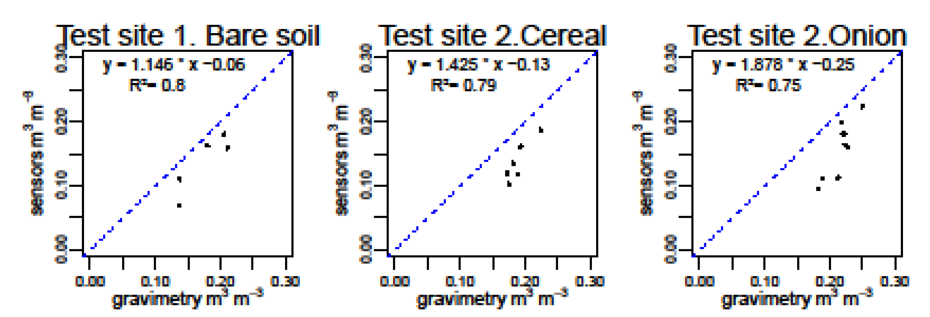
2.6. Soil Moisture Ground Measurements

At the center of each experimental field, an SSM station was installed on 8 October 2020, for Test site 1: Bare soil, on 10 December 2020, for Test site 2: Cereal plot, and on 2 March 2021, for Test site 2: Onion plot. SSM was continuously measured every 15 min using six sensors, TEROS 10, capacitive type, connected to METERS’ ZL6 six-channel loggers with integrated GPS and ZENTRA application, which can be accessed from computers or smartphones (Figure 4). The sensors and data logger came from the METER Group manufacturer (METER Group AG, München, Germany). Five sensors were set up at 5 cm and only one sensor at 25 cm at Test site 1. For the comparisons to the Sentinel 1 data, only the in situ measurements of topsoil (5 cm) moisture content were used in this study. Data were extracted whenever the C-SAR Sentinel 1 images were available. In the study region, these images were taken only at the ascendant of the satellite flying over the study area at 18:00 UTC. Therefore, only the average of the SSM values recorded at 18:00 UTC by the five sensors installed at 5 cm was used.
At Test site 2: Cereal, SSM was continuously measured every 15 min and the six sensors were placed at 5 cm. At Test site 2: Onion, four sensors were installed at 5 cm, one at 15 cm and the last at 20 cm. No soil moisture sensors were set up at Test site 2: Peas 1 and Peas 2.
For Test site 2: Cereal, Peas 1, Peas 2 and Onion, Sentinel 1 images were acquired whenever the satellite flew over the study area at 18:00 UTC. Hence, the average of the SSM values recorded at 18:00 UTC was used.
In addition to the SSM stations installed in the cereal and onion experimental fields, other in situ soil measurements were taken by the classic gravimetric method. The acquisition time of the gravimetric samples always fell within a 2 h range during the radar overpass event. Five, seven, six and seven gravimetric samples were taken in the cereal field, the peas 1 field, the peas 2 field and the onion field, respectively. These gravimetric soil samples were always taken at the same location to mitigate the effects of any variation from sampling errors and to enhance the measured SSM precision. A handheld GPS (Leica, Zeno, Wetzlar, Germany) was used, with an average accuracy of 2 cm, to obtain the exact coordinate of each sample point.
Every sample was transferred to a metal recipient and placed in a stove at 105 °C until dry weight stabilized and stopped changing. The following formula was applied to estimate gravimetric SSM:
V 0 = V w V d   V d   g / g
where V 0 is the gravimetric soil water content, V w   is   wet   weight   and   V d is dry weight.
Volumetric SSM was expressed as:
V V = V 0 ρ H 2 O   B D     unit   of   volume unit   of   volume
where V V is volumetric soil water content, ρ H 2 O is water density and BD is the bulk density of the soil sample.
TEROS 10 sensors were calibrated with gravimetric acquisition. Calibration was performed using the samples taken from Test site 1 and Test site 2: Cereal and Test site 2: Onion. In each field, many samples were collected on different days, which were chosen with various SSM conditions to cover a wide range of SSM values. The linear regression established between the volumetric water content obtained by the gravimetric method, and the volumetric water content acquired by TEROS 10 at the Test site 1 and Test site 2: Cereal and Onion fields, are presented in Figure 5.
During the 2020–2021 SSM measurement field campaign, at Test site 2, the phenological growth stage according to the BBCH (Biologische Bundesanstalt, Bundessortenamt und CHemische Industrie) [33] scale was recorded.

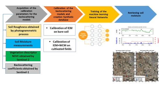
2.7. Retrieving Soil Moisture

In order to invert the backscattering values obtained by the backscatter model (or models) and to retrieve SSM, many algorithms have been used, such as NN [21,23], support vector machine (SVM) [34] and Look-up Tables [35]. In the present study, the approach applied to retrieve SSM was based on the methodology described in [22]. We applied the multilayer NN algorithm to invert the VV SAR signal. We decided to use only VV polarization because the authors of [22] confirmed that VV alone provides more accurate SSM estimates. NN were trained using a synthetic database of the C-band backscattering coefficients and SSM. The synthetic database was built using only the IEM for the Test site 1 experimental field, and the WCM combined with IEM for the Test site 2 experimental fields (Figure 6). The main steps of the methodology with the retrieving process were: (1) simulation of radar backscattering coefficients of VV using only the IEM for Test site 1, and both the IEM and WCM for Test site 2, respectively, (2) training and validation of NN with the synthetic trained and validated sub-databases, respectively, and (3) application of the trained NN to the actual database with only VV to estimate SSM. Soil texture characteristics (sand fraction, clay fraction, BD, soil temperature) are necessary to transform SSM values into dielectric constants.
In order to retrieve SSM, NN were employed. The structure of NN was composed of an input and output. NN had a two-dimensional input vector. The one-dimensional output vector contained SSM. Data were subdivided into a training and a validation dataset, always with 70% for the training dataset and the remaining 30% for the accuracy estimation to run the NN algorithm. These subgroups were obtained by following an iterative random process, which ensured that the training and validation datasets had the most similar mean and standard deviation. NN were trained with the backscattering coefficient data generated from the backscattering models, and were validated using the radar data. In an NN, a hidden layer is considered to be a layer in between the input and output layers. In this study, the number of neurons utilized in the hidden layer was generally between 6 and 8.

2.7.1. IEM (Integral Equation Model)

The IEM is a mathematically sophisticated computational algorithm that was developed in [36] as a theoretical backscatter model. It computes the backscattering or the bistatic scattering of a wide range of roughness scales (from smooth to rough surfaces), and for any combination of receiver or transmitter wave polarization [37]. Therefore, given its mathematical background and solid theoretical physical basis, it is considered the most critical backscatter model for bare soil surfaces. It is used in inversion procedures to retrieve SSM and/or roughness parameters [11]. The IEM takes soil status into account with input parameters, such as soil moisture, hrms, L and the L shape or function [36]. Several studies have been performed by applying the IEM. The authors of [38] retrieved SSM from ASAR C-band data at several incidence angles.
The backscattering coefficient of the surface contribution is expressed on bare soils in agricultural areas at VV or HH polarization, as in [6]:
σ p p 0 = k 2 2 | f p p | 2 e 4 r m s 2   k 2   c o s 2 θ n = 1 + ( 4 h r m s 2   k 2 c o s 2   θ ) n n ! W ( n ) ( 2 k s i n θ ,   0 ) + k 2 2 R e ( f p p * F p p ) e 3 r m s 2   k 2   c o s 2 θ n = 1 + ( 4 h r m s 2   k 2 c o s 2   θ ) n n ! W ( n ) ( 2 k s i n θ ,   0 ) + k 2 8 | F p p | 2 e 2 r m s 2   k 2   c o s 2 θ n = 1 + ( h r m s 2   k 2 c o s 2   θ ) n n ! W ( n ) ( 2 k s i n θ ,   0 )
where:
f V V = 2 R v c o s θ
F v v = 2 s i n 2 θ c o s θ [ ( 1 ε r c o s 2 θ μ r ε r s i n 2 θ ) ( 1 R v ) 2 + ( 1 1 ε r ) ( 1 + R v ) 2 ]
R v = ε r c o s θ μ r ε r s i n 2 θ ε r c o s θ + μ r ε r s i n 2 θ   Fresnel   coefficient   at   vertical   polarization
where   W ( n ) is the Fourier transform of the nth power of the surface correlation coefficient, ε r = dielectric constant, which is obtained based on volumetric water content using the empirical model of [39], μ r = relative permitivity, θ = incidence angle, hrms = standard deviation of surface height, L = correlation length, polarization (pp with p = V), Re = real part of the complex number, f * pp = conjugate of the complex number fpp and ρ (x, y) = surface correlation function.
In this study, the employed correlation functions were defined as follows [11]:
ρ ( x ) = e ( x L )

2.7.2. WCM (Water Cloud Model)

The WCM was developed by Attema and Ulaby in 1978 as an approach to characterize the scattering contribution of the canopy volume [40]. This model simplifies the complex scattering effect between the vegetation layer and the soil layer [41], and is appropriate for different vegetation layer types. The WCM assumes that the vegetation layer is a uniform medium, and the canopy can be represented with one vegetation parameter or two [42]. The WCM has been widely used in different studies with various frequencies and incidence angles [43,44].
The polarization applied in this study was VV. The WCM defined the backscattered radar signal on a linear scale ( σ t o t 0 ) as the sum of the contribution from vegetation ( σ v e g 0 ), oil ( σ s o i l 0 ) attenuated by vegetation ( T 2 σ s o i l 0 ) and multiple soil-vegetation scatterings:
σ t o t . v v 0 = σ v e g . v v 0 + T 2 σ s o i l 0
σ v e g . p q 0 = A v v V 1 c o s θ ( 1 T V V 2 )
T p q 2 = e 2 B v v V 2 s e c θ
where V 1 and V 2 are vegetation descriptors. In this study, V 1 = V 2 = NDVI, as in [43], θ is the radar incidence angle, parameters A V V and B V V were estimated for VV by minimizing the sum of the squares of the differences between the simulated and measured radar signals, T V V 2 is two-way attenuation and σ s o i l 0 was estimated in a previous step by the IEM.

2.8. Remote Sensing Data: Sentinel 1 and Sentinel 2 Dataset

2.8.1. Sentinel 2 Dataset

Sentinel 2 products were acquired on different dates during the 2020–2021 period. For each acquisition date, we downloaded a different Sentinel 2 tile, SWJ. The Sentinel 2 products at level 2A Bottom Of Atmosphere (BOA) were downloaded from the ESA, Copernicus Open Access Hub. The NDVI at the Bottom Of the Atmosphere (NDVIBOA) was calculated by the following equation:
N D V I B O A = Band   8 Band   4   Band   8 + Band   4
In order to obtain the vegetation condition of each experimental field, the NDVI pixel values in each reference plot were averaged.

2.8.2. Sentinel 1 Dataset

Sentinel 1 images were acquired during the 2020–2021 period. The incidence angle of Sentinel 1 over the study site was about 38.5°. The Sentinel 1 dataset comprised the level 1 Ground Range Detected (GRD) data in the interferometric wide (IW) swath mode, which was projected to the ground range by the WGS84 Earth ellipsoid model. The dimensions of the resulting images in dual-polarization (VH and VV) were 270 × 270 km, with a resolution of 10 m and a temporal resolution of 6 days. All the images were processed by SNAP using the Sentinel 1 toolbox. The main performed corrections were: (1) radiometric calibration, (2) speckle filtering and (3) geometric correction. Finally, conversion into decibel units was performed: backscatter coefficient, σ 0 , on a linear scale, was converted into the decibel (dB) scale, σ 0 ( d b ) = 10   log 10   σ 0 , where σ 0 ( d b ) represents the backscatter coefficient value.

2.9. Statistical Evaluation of Models

The root mean square error (RMSE) was considered to estimate models’ precision, as:
R M S E = i = 1 n ( A t F t ) 2 n
The RMSE is the square of the sum of squared errors, divided by the number of observations, where n is the number of data samples, F t is the forecasted value of sample I and A t is the observed or actual value of sample i.

3. Results

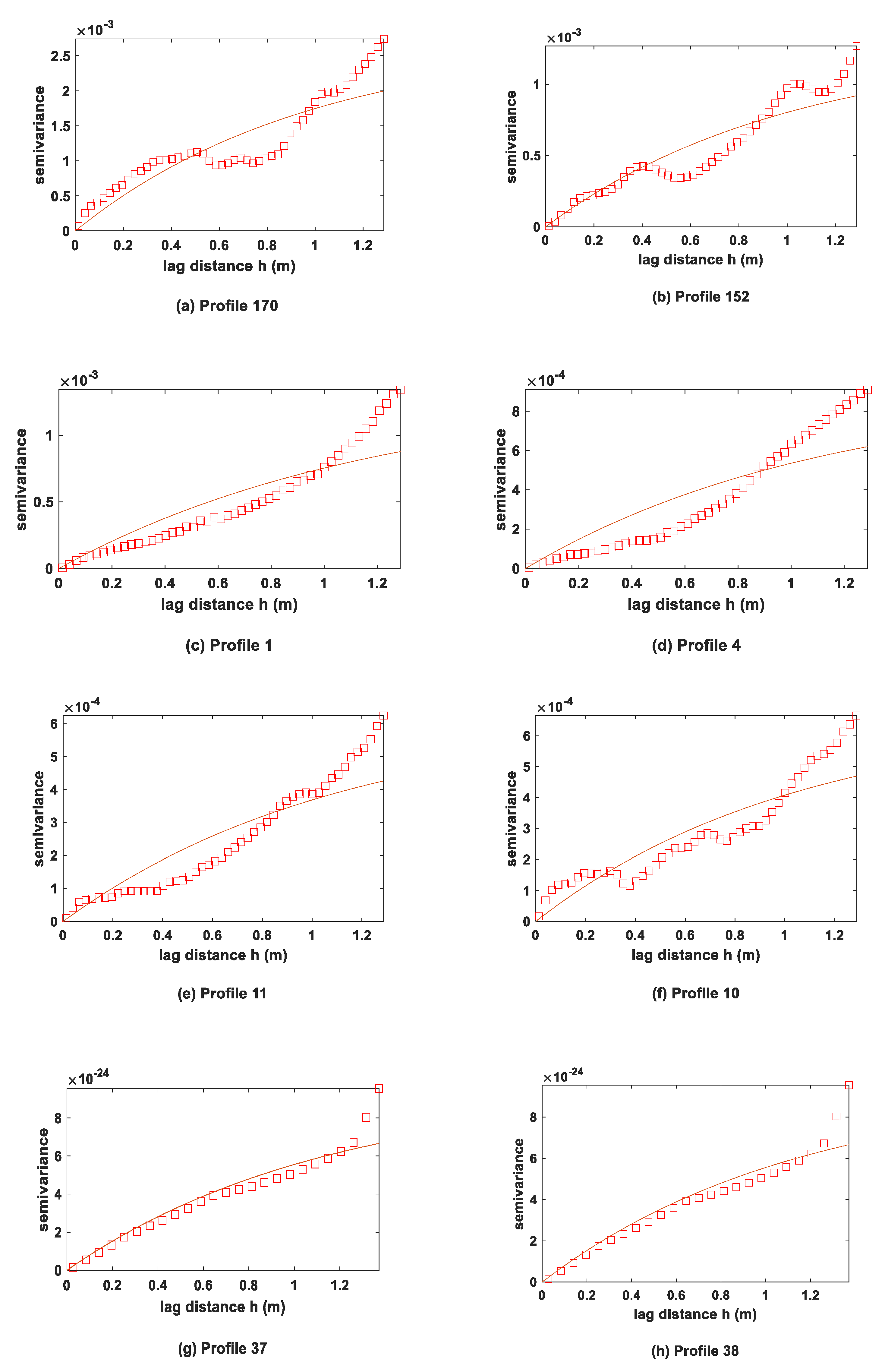
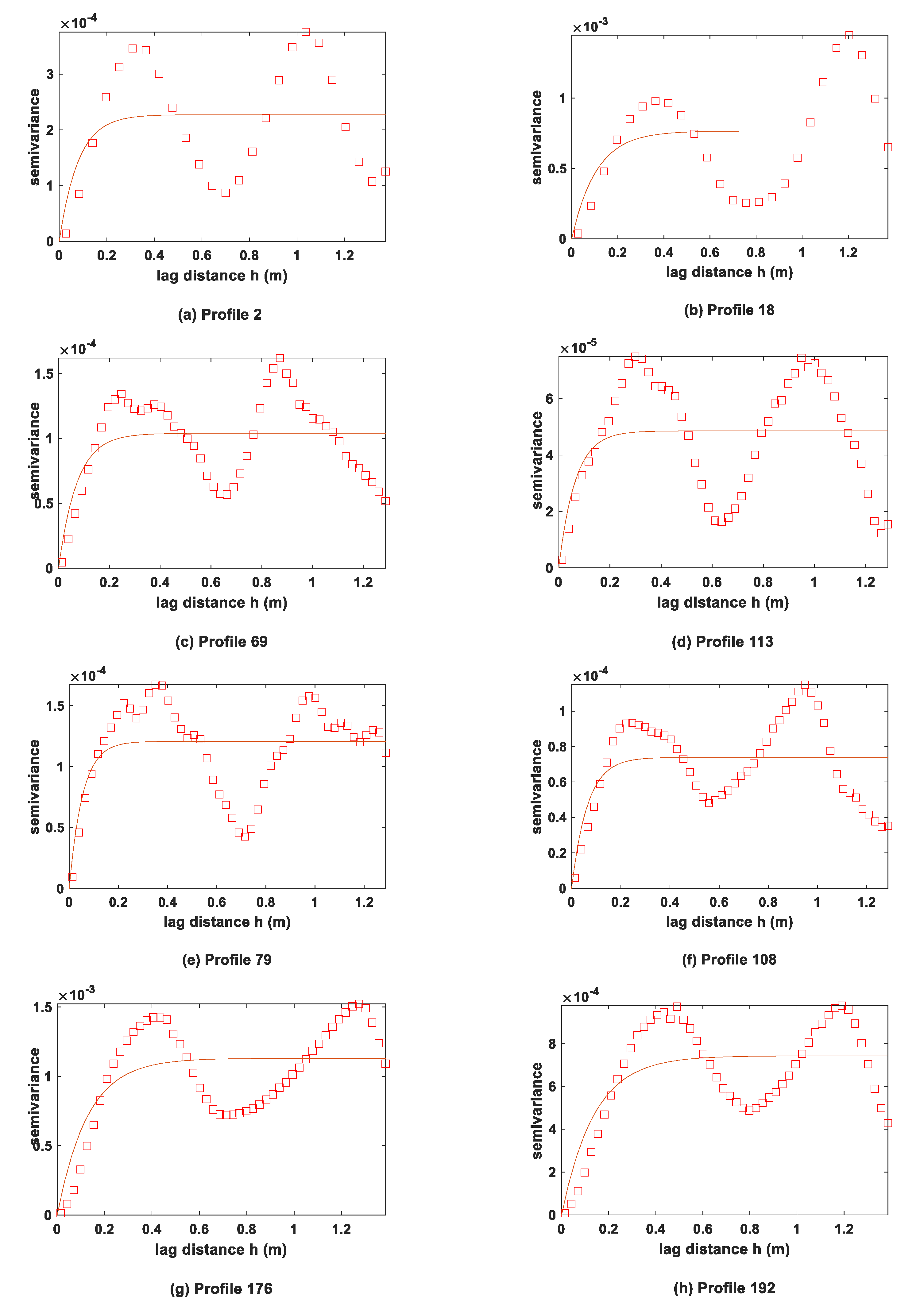
3.1. Example of Variograms of Roughness Showing a Spatial Trend and a Significant Two-Scale Roughness Pattern

Figure 7 depicts an example of the variograms obtained from the profiles showing a spatial trend: profiles (a) and (b) taken from the Test site 1 experimental field, profiles (c) and (d) taken from Test site 2: Peas 1, profiles (e) and (f) taken from Test site 2: Cereal and profiles (g) and (h) taken from Test site 2: Onion. The natural soil surface was assumed in most cases to be isotropic, and described to be a single-scale process [14]. In the agricultural field, tillage practices induced a systematic pattern known as oriented roughness. This anisotropic roughness pattern can be statistically described as the sum of two phenomena [45]: a small-scale roughness pattern (e.g., seedbed rows, soil clod distribution) and a large scale component (e.g., wheel tracks).
Figure 8 illustrates examples of the variograms extracted from Test sites 1 and 2 that, in turn, illustrate the two-scale roughness pattern observed in the tilled agricultural field. In the study conducted in [18], the authors used a variogram to decompose and characterize the soil surface on different scales. From the variogram, they determined the distance within a range corresponding to wheel tracks, and they defined the distance threshold that allowed to mask out wheel tracks. In our work, we applied the same methodology. As Figure 8 shows, we defined these different variograms, and their corresponding surfaces displayed a repetitive behavior for distances within a range from 0.6 to 0.7 m, which corresponded to wheel tracks. We intended to comprise the random appearance of soil with the seedbed rows (as a general range, the row spacing for cereal and peas is about 10 cm, and for onion varies between 11 and 15 cm) in one class separate from the wheel tracks.

3.2. Roughness Parameters’ Values

The application of the described methodology allowed us to obtain Table 3. For each experimental field, the mean of both L ¯ and h r m s ¯ was computed by averaging the individual L and hrms of the obtained profiles. For Test site 1 and Test site 2: Onion, the hrms values were higher than 2 cm. These roughness values can be explained by the Test site 1 field having well-plowed soil, and the onion field being prepared in flat planks of about 50 cm wide, separated by channels to allow circulation and irrigation. For the cereal and peas 1 fields, the hrms values were lower than 1 cm because the roughness parameters were measured immediately after sowing, and fields were smooth areas. It is worth mentioning that no soil work was carried out after sowing. Therefore, we assumed that there were no significant changes in hrms and L, and the roughness effect on the radar signal did not change during the measurement campaign, but was considered the same for all the experiment periods.

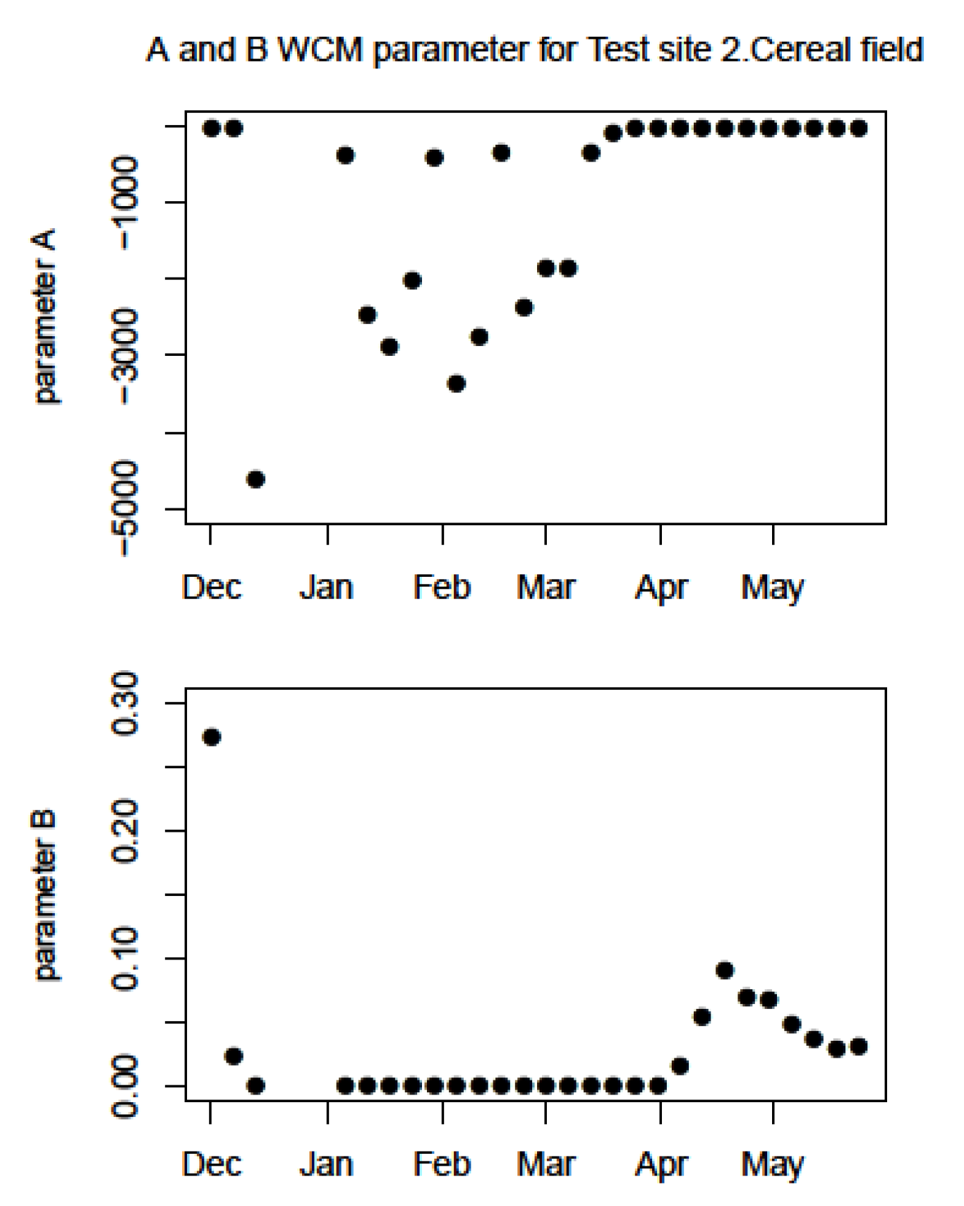
3.3. WCM Optimizations Parameters

As previously mentioned, parameterization consisted of fitting the model to the ground measurements (Equations (14) and (15)). We processed the data weekly from when the experimentation began, and we evaluated evolution on a weekly basis. For example, the WCM optimization parameters (A and B) throughout the experimentation period of Test site 2: Cereal are presented in Figure 9, respectively. Table 4 presents the A and B values when modeling the relation between the simulated and observed backscatter coefficients at VV polarization was optimal.

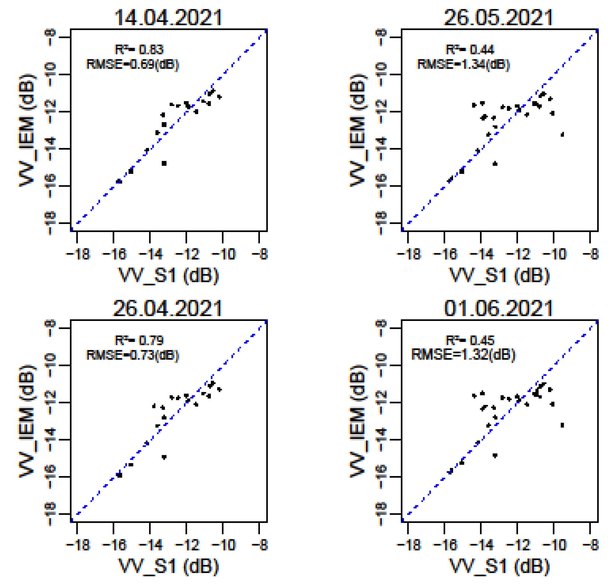
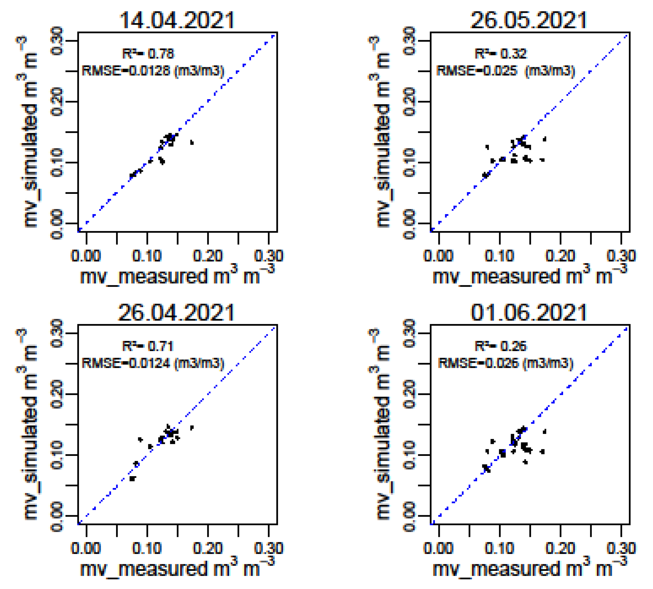
3.4. Results of Test Site 1: The Bare Soil Case

In this section, we present the simulation results of the backscatter coefficients of the IEM scattering model at VV polarization at the agricultural bare soil Test site 1 by applying the methodology described in the previous section and using the measured roughness parameters L ¯ and h r m s ¯ and the exponential distribution of the correlation function. This experimentation lasted 8 months, from October to May, and we used 35 Sentinel 1 images, as presented in Figure 10, which also presents the meteorological conditions during this experiment (precipitation and temperature).
Figure 11 shows the relation between the backscatter coefficients at VV polarization deriving from Sentinel 1 and simulated by the IEM for two different dates: 26 April and 26 May 2021. The objective of presenting the relation for these two dates was to demonstrate that the relation between the observed VV_S1 and the simulated VV_IEM did not change in the last experimentation month because we processed data weekly from the time when experiments began, and we took note of any evolution in the relation weekly. We observed no notable variation in the last month. R2 was equal to 0.76 on 26 April and 0.75 on 26 May, both in 2021.
.
The relation between the simulated and observed VV was statistically evaluated with RMSE. According to these results, we noted only a slight difference between the compared indicator on these two dates, which confirmed that the relation had become stable in the last experimentation month to a certain extent. Likewise, based on this analysis, we can clearly see that the IEM with the measured roughness parameters correctly simulated the radar signal at VV polarization because the RMSE between VV_S1 (Sentinel 1) and VV_IEM (simulated by the IEM) was equal to 0.52 dB on 26 April and 0.54 dB on 26 May, both in 2021.
Figure 12 compares the retrieved moisture with the measurement obtained from the sensor from Test site 1 for both dates (26 April and 26 May 2021). We can see that R2 on 26 April was slightly higher than on 26 May, with 0.74 and 0.72, respectively. RMSE was equal to 0.024 and 0.023 m3/m3 on 26 April and 26 May, respectively.

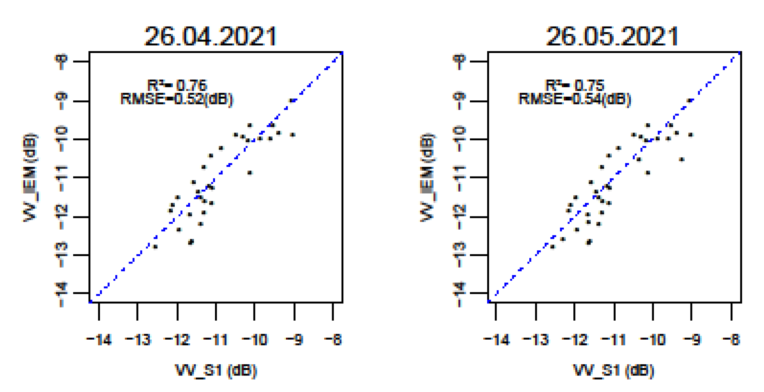
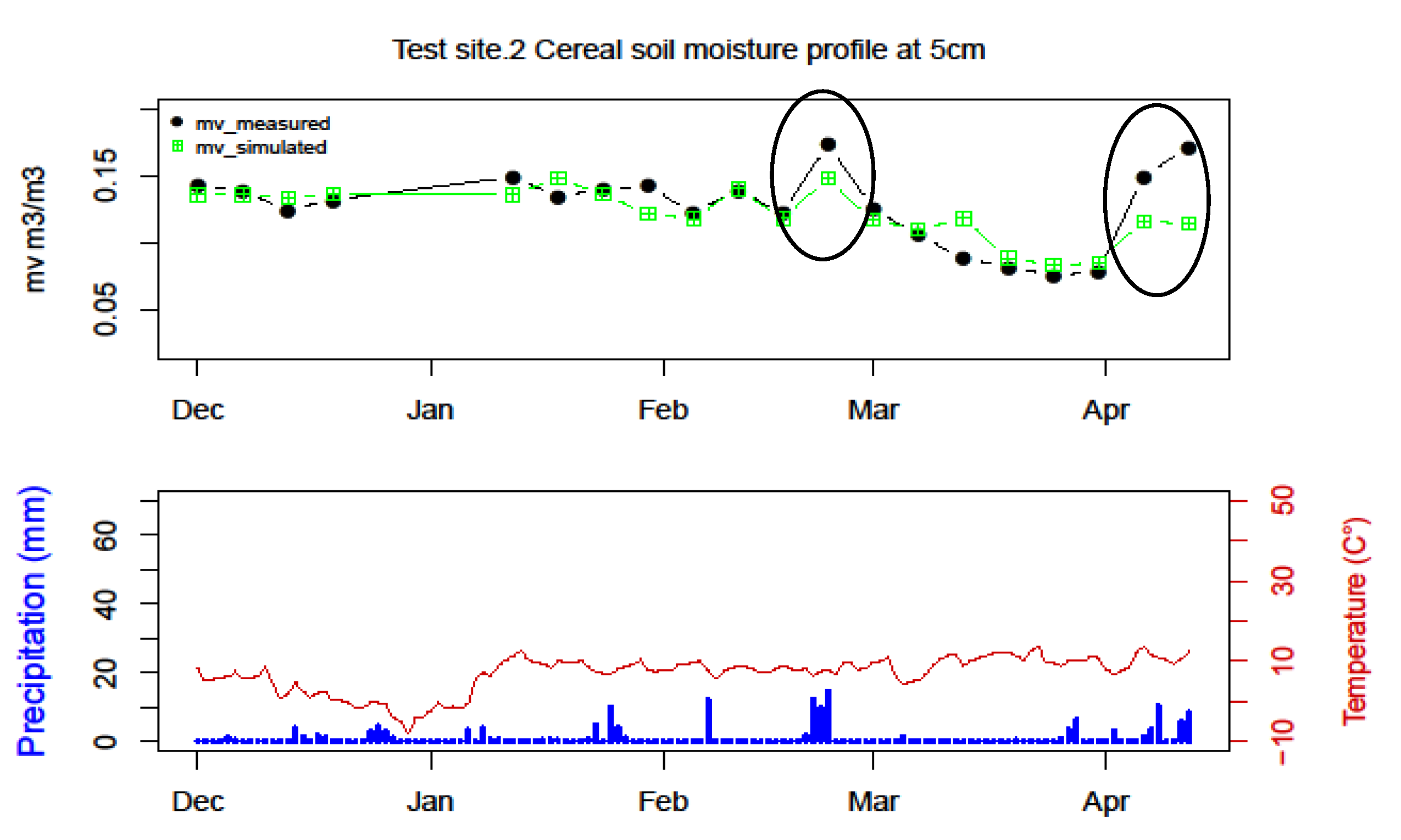
3.5. Cereal Crop Results

We now present the simulation results of the backscatter coefficients of the IEM combined with the WCM scattering models at VV polarization on the experimental barley field after applying the methodology described in Figure 6 and using the measured roughness parameters L ¯ and h r m s ¯ . This experimentation lasted 6 months, from 15 December to 1 June. We used 26 Sentinel 1 images to extract the observed VV and 26 Sentinel 2 images to extract the NDVI, as presented in Figure 13.
Due to bad weather conditions, Sentinel 2 acquisition was sometimes covered by cloud, which led to missing data. In January, a snowstorm named “Filomena” arrived and lasted more than one week. Due to the cold weather, snow lasted two more weeks and we were unable to use the Sentinel 1 data because the observed backscattering value at VV polarization was affected by snow. As recommended in [46], snow data should be removed from the dataset because frozen conditions, wet snow and intercepted rain can disturb σ 0 observations.
Figure 14 displays the relation between the simulated backscatter coefficient at VV polarization using the combined models IEM and WCM and the observed Sentinel 1 data on four dates during the experimental period (14 April, 26 April, 26 May, 1 June). These dates were chosen to show that backscattering coefficient modeling evolution was also related to phenological crop cycle evolution. The optimums, which corresponded to the highest R2 (between 0.83 and 0.79) (Figure 14) and the lowest RMSE (between 0.69 and 0.73 dB), were obtained between mid-April and the end of April, which corresponded to the crop heading stage (around 45 on the BBCH scale). After reaching the optimum, the modeling results started to deteriorate. The explanation for this observed deterioration could be due to changes in the canopy structure [47,48]. Since then, crop development has created a kind of top layer that obstructed radar signals from passing to soil. Consequently, the Sentinel 1 radar signal penetrated only this layer, resulting in increasing volume scattering, while attenuation became lower [49,50]. Therefore, the difference between the observed backscattering coefficient provided by Sentinel 1 and the simulated one provided by the IEM combined with the WCM commenced from this stage.
Figure 15 compares the moisture retrieved with the measurement taken from the sensor in the experimental field on four dates: 14 April, 26 April, 26 May and 1 June. Overall, the results showed that R2 decreased slightly from 14 to 26 April, and went from 0.78 to 0.71, respectively, but drastically dropped on 1 June, with R2 being 0.26. Furthermore, the RMSE indicated no significant difference between 14 and 26 April, nor between 26 May and 1 June.

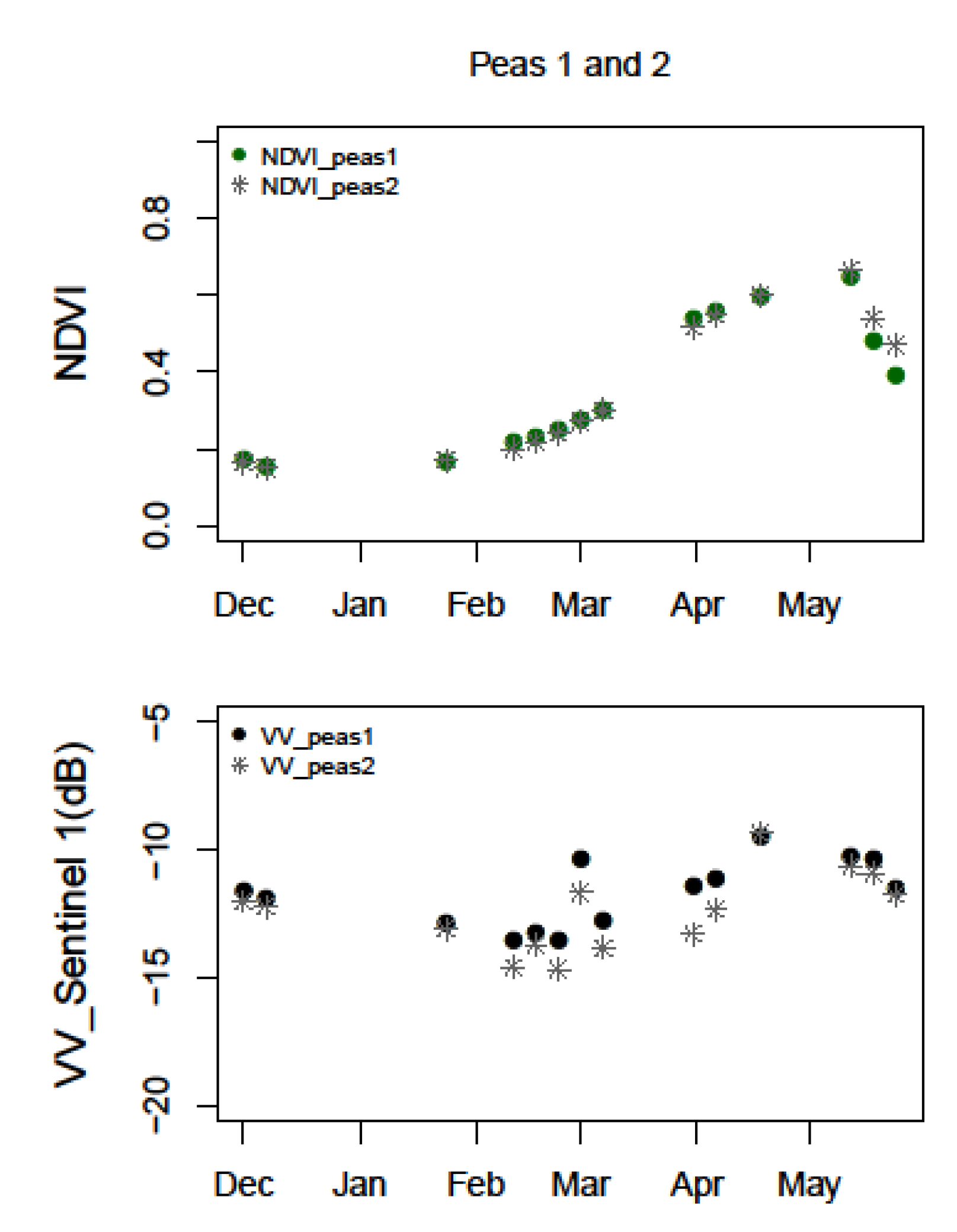
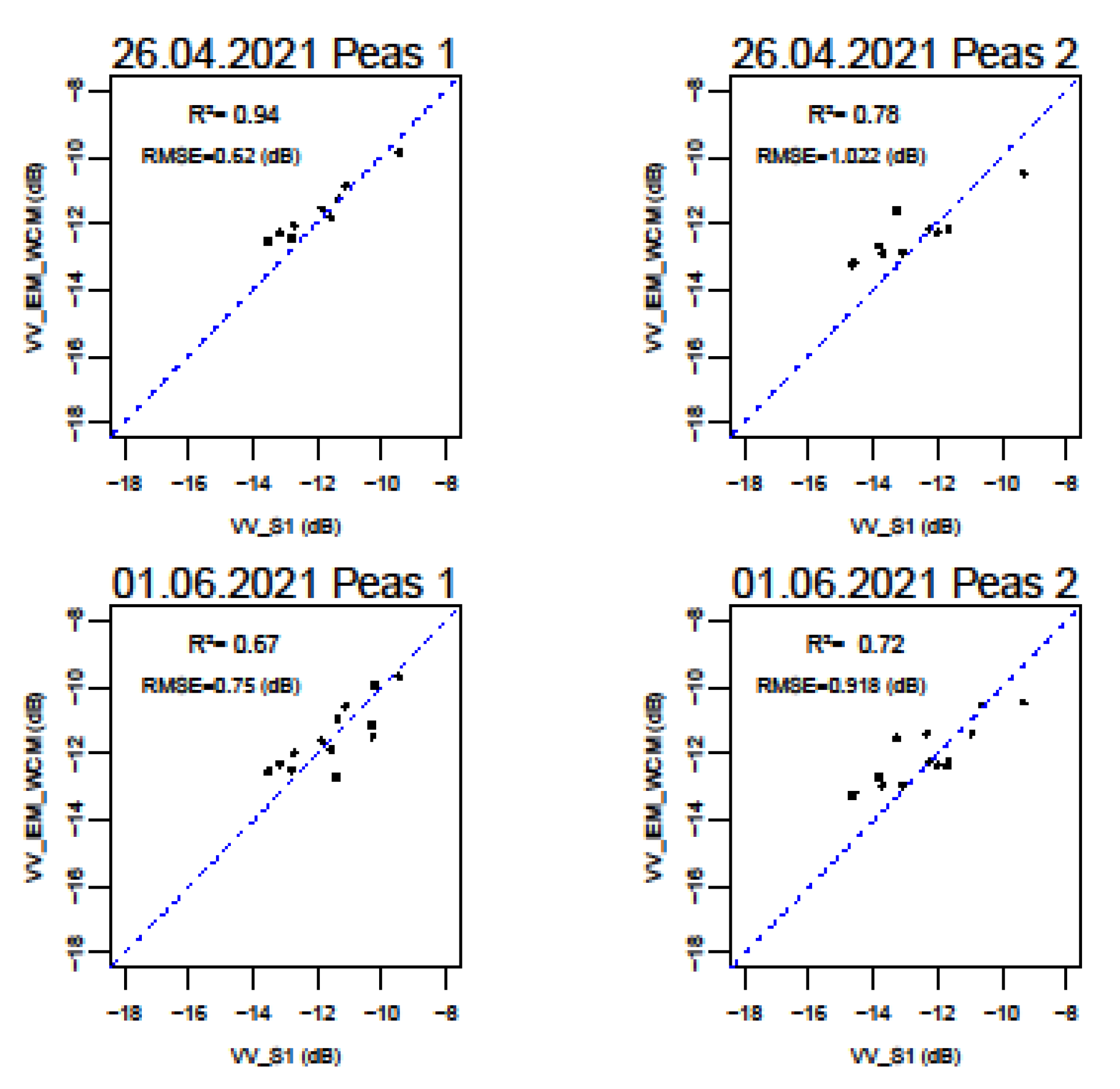
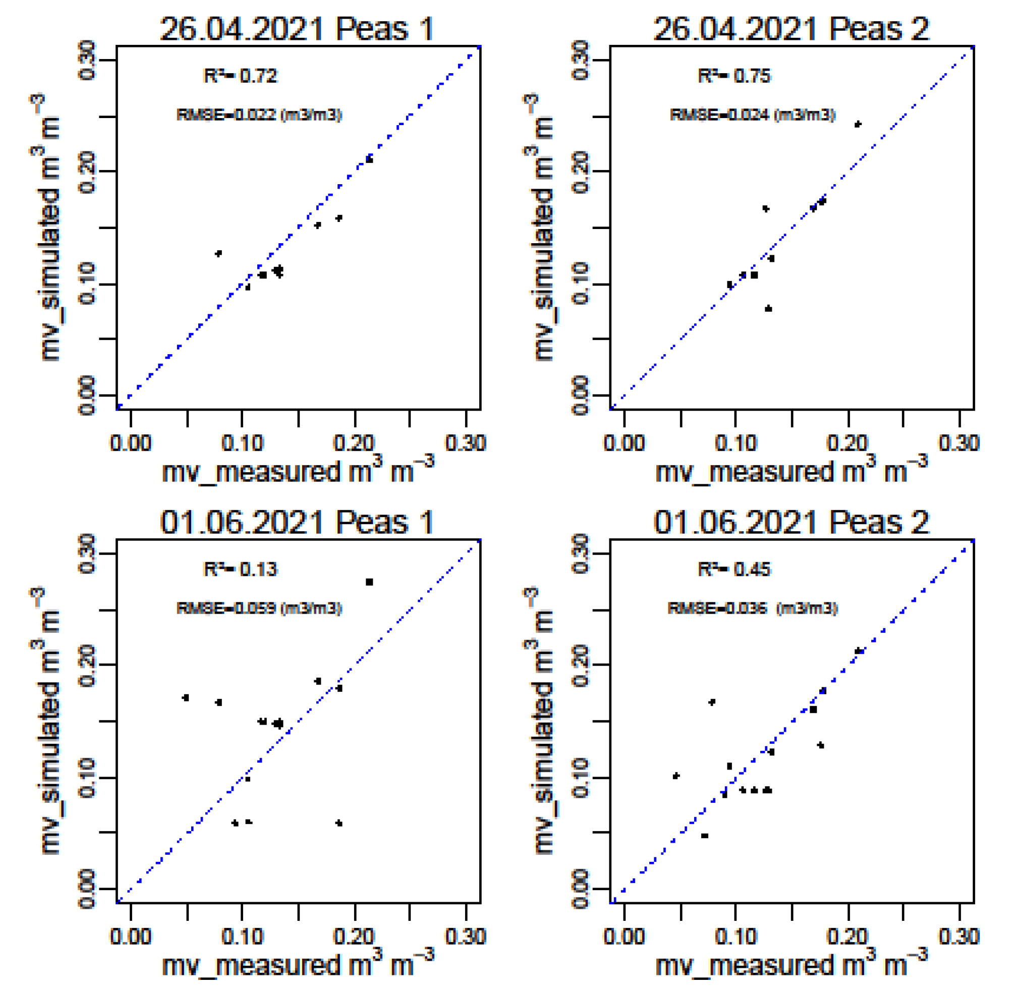
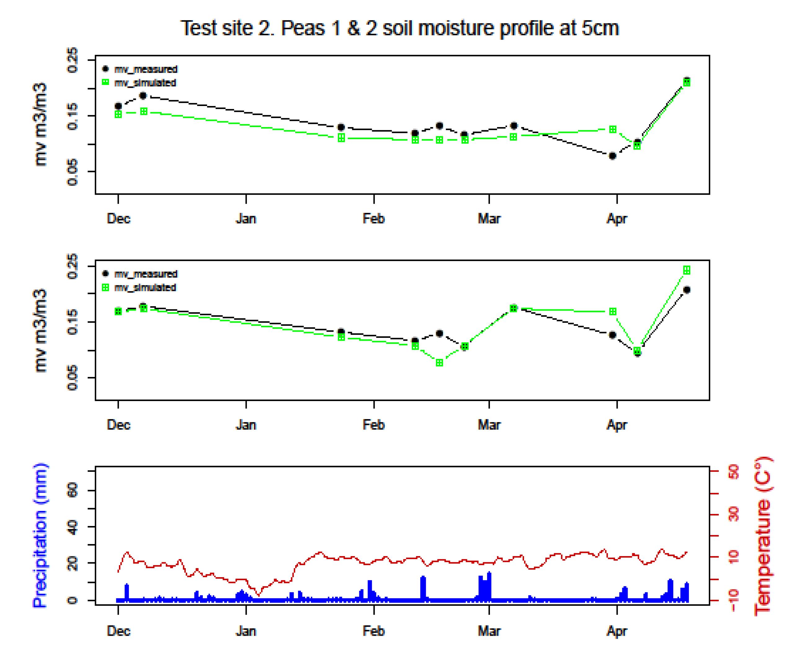
3.6. Peas Crop Results

In this section, we present the simulation results of the backscatter coefficients of the IEM combined with the WCM scattering models at VV polarization over Test site 2: Peas 1 and Peas 2. Over peas 1, we measured roughness parameters L ¯ and h r m s ¯ . In peas 2, we applied the same parameters obtained in peas 1. This experimentation lasted 6 months, from 15 December to 1 June. We used 14 Sentinel 1 images to extract the observed VV (shown in Figure 16), and 9 Sentinel 2 images to extract the NDVI. Only gravimetric samples were taken, which explains the gap period in the VV Sentinel 1 and NDVI dataset because data were acquired only on working days.
Figure 17 displays the relation between the simulated backscatter coefficient at VV polarization using the combined IEM and WCM and Sentinel 1 observed on two dates during the experimental period (26 April and 1 June) for the two experimental fields peas 1 and 2. Over the experimental field peas 2, we applied the same roughness parameters L ¯ and h r m s ¯ that were measured over peas 1. The same number of Sentinel 1 and 2 data were used for peas 1 and the same number of gravimetric measurements were performed. The same observation as with the cereal field was made. For peas 1, we stress that backscattering coefficient modeling evolution was also related to phenological crop cycle evolution: the optimum corresponded to the highest R2 = 0.94, and the lowest RMSE at 0.62 dB was obtained on 26 April, which corresponded to phase 6 of the BBCH scale. After reaching the optimum, the modeling results representing the relation between the observed and simulated backscattering coefficient started to deteriorate until 1 June with an R2 of 0.67 and an RMSE of 0.75. For peas 2, and according to the results in Figure 17, the application of the same roughness parameters as in peas 1 allowed us to obtain similar results. This observation can be explained by both plots having sustained the same tillage work.
Figure 18 compares the moisture retrieved to the measurement obtained with the gravimetry measurements taken in experimental fields peas 1 and 2 on two dates: 26 April and 1 June. For peas 1, despite the relation between the simulated backscatter coefficient at VV on 1 June being R2 = 0.67, the inversion of the model resulted in a poor relation as R2 was 0.13. Unlike the model inversion of peas 1 on 1 June, peas 2 had a relatively high R2 of 0.45.

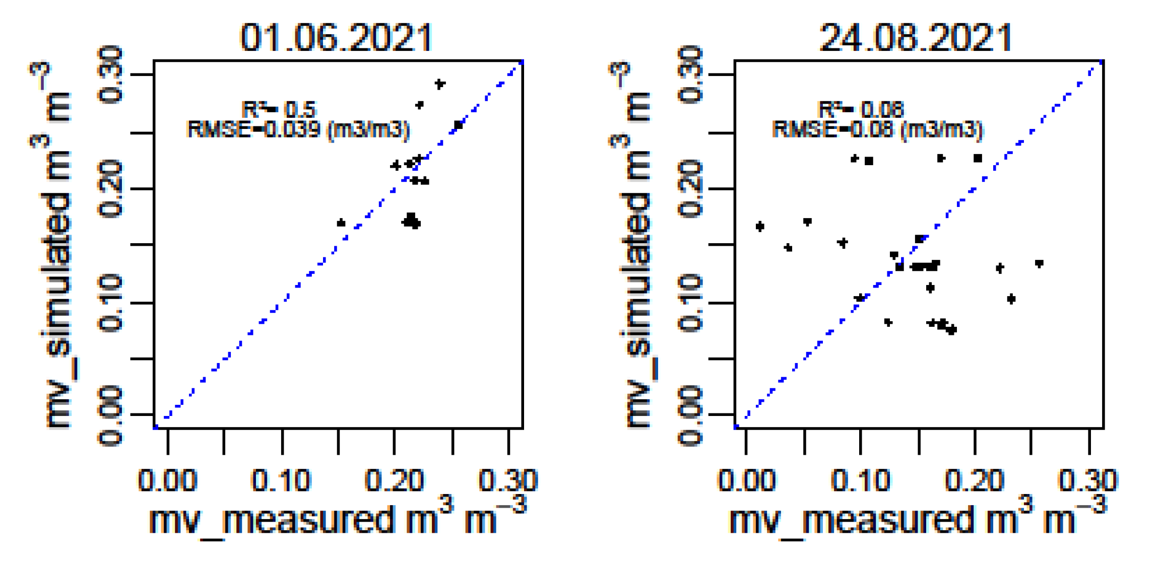
3.7. Onion Crop Results

As in the barley and peas 1 and 2 experimental fields, we simulated the VV backscatter coefficient by integrating both the IEM with WCM, and by applying the same methodology and using the measured roughness parameters L ¯ and h r m s ¯ . This experimentation lasted 6 months, from 9 March to 24 August. We used 29 Sentinel 1 and Sentinel 2 images to extract the observed VV and the NDVI, as presented in Figure 19.
Figure 20 exhibits the relation between the observed and forecasted backscatter coefficient at VV polarization for two dates: 1 June and 24 August. We noted that backscattering coefficient modeling evolution reached the optimum, which corresponded to the highest R2 = 0.54 with RMSE = 0.8 dB and reached the minimum at the end of the growing cycle, with R2 = 0.14 and RMSE = 1.98 dB. 2 June corresponded to the leaf development stage and the sixth leaf was clearly visible, while 23 August coincided with complete crop growth.
Figure 21 compares the moisture retrieved with the measurement obtained from the sensor in the experimental field for two dates, 1 June and 24 August. According to the results, R2 drastically dropped from 0.5 to 0.08, and RMSE increased from 1 June to 24 August from 0.039 to 0.08, respectively.

4. Discussion

4.1. Analysis of the New Procedure to Obtain hrms and L

The study conducted in [51] was performed over experimental cereal (wheat) fields for three years. Measurements were taken with a pin profiler. According to that work, the range of h r m s ¯ measurements lay between 0.83 and 1.35, with L ¯ between 5 and 7.4 cm. In another study [52] performed over cereal plots, the h r m s ¯ measurements were between 0.46 and 6.46, and L ¯ went from 2.8 to 10.11 cm. Therefore, when we compared the values of our cereal experimental field to those of the aforementioned studies, we found that our calculated h r m s ¯ fell within the value range, but L ¯ was slightly higher than the obtained range. This small difference could be due to many factors, such as how measurements were taken, the calculation methodology, tillage work, the tilling field used and the soil type. We believe that all these elements could have resulted in this small difference.
Based on their 20-year experience in collecting roughness measurements values, the authors of [22] classified roughness values into three main classes: smooth areas (sowing) with an hrms below 1 cm, medium roughness areas (slightly plowed soil) with an hrms between 1 and 2 cm and rough areas (well-plowed soil) with an hrms above 2 cm. Hence, it seems that this classification well-matches our obtained h r m s ¯ because the h r m s ¯ for the pea and barley plots was lower than 1, field soil was well-plowed in the Test site 1 with h r m s ¯ = 2.1 and the onion field was considered a rough area because it was prepared on very flat planks (about 50 cm wide) separated by channels to allow circulation and irrigation.
The proposed methodology facilitates the procedure to obtain accurate L and hrms values. This helps the applicability of this procedure to obtain SSM from SAR information. It can also lead to new works being conducted, whose aim is the standardization of these required values depending on tillage and soil type, among many other factors.

4.2. Bare Soil Results

We can generally confirm that simulating the IEM over bare agricultural plots using the roughness parameters measured by photogrammetric techniques provided very promising results compared to previous works, which have also used the IEM [34,53,54,55]. In fact, in our case study, the RMSE and R2 obtained between the simulated and Sentinel 1 backscattering coefficients at VV polarization on 26 May were about 0.54 and 0.75 dB, respectively. This agrees with previous studies that have reported statistical indicators within the same range. For instance, the authors of [34] found that RMSE was 1.7 dB and R2 was 0.7. Similarly, the authors of [55] employed the calibrated IEM [56,57,58] by replacing L with Lopt. That calibration consisted of replacing the measured correlation length with a fitting parameter Lopt, which depends on hrms, θ , radar wavelength and polarization [23]. Those authors reported results for the comparison between the σ 0 values extracted from the Sentinel 1 and estimated data, and found that RMSE was 0.78 and R2 was 0.9. For the IEM’s potential for the measured roughness parameters to forecast SSM from the Sentinel 1 backscattering coefficient, we obtained satisfactory results, with RMSE of 0.023 m3/m3 and R2 of 0.72 on 26 May. In addition, these results could be further improved if L and hrms were calculated throughout experimentation to capture all variations (rain, wind, etc.) on bare soil and to know their influence on the roughness parameters. However, calculating these parameters throughout experimentation would reduce the methodology’s applicability.

4.3. Field Crop Results

The observations made in [58] also confirmed that backscattering coefficient modelling evolution was related to crop cycle evolution. They showed that the sensitivity of σ 0 to SSM decreased with the NDVI between 0.45 and 0.90. This effect appeared as vegetation (cereal and peas) started to increase at the beginning of February, which corresponded to not only the tillering stage until mid-April, but also to the stem elongation period. As a result of such vegetation development, the VV backscatter signals decreased due to the rising attenuation from the predominantly vertical structure of barley stems [59], and decreasing the soil contribution was similar to increasing the vegetation contribution σ 0 , with slight decreases with increases in the NDVI until a minimum was obtained [60]. Until the end of April, the Test site 2 cereal results showed that the IEM-WCM combination adequately simulated SAR observations (RMSE = 0.73 dB).
As the main objective of retrieving SSM over agricultural fields is essentially precise irrigation management, this approach should be implemented regularly throughout the growing season. Plants are very susceptible to damage caused by water deficiency in vegetative and reproductive growth stages [1,60]. In [61], the authors exhibited modeling results in the most important growth stages of cereal fields. The soil water content retrieval results upon the harvest of winter wheat showed the best accuracy of three field experiments (R2 = 0.66; RMSE = 2.24%), followed by the tillering stage (R2 = 0.56; RMSE = 2.56%) and jointing stage (R2 = 0.36; RMSE = 2.74%). According to our results, the best accuracy was obtained in the stem elongation stage from 14 April to 26 April (R2 = 0.78), but it significantly diminished at harvest, with R2 = 0.26 on 1 June. In [61], the authors calibrated the WCM and found that calibrated parameter A first increased and then decreased, whereas parameter B first decreased and then increased, in the growth cycle. However, in our study, parameter A decreased in the first phases, and then decreased again to finally remain almost constant, and continued to be almost constant until the end of April. Then, it increased and decreased in the final stage. The differences between these two parameters’ evolution behaviors can be explained by the fact that in [61], the vegetation descriptor used to calibrate the WCM was the LAI (Leaf Area Index) simulated by the SAFY (Simple Algorithm For Yield) estimate.
The simplicity of parametrizing the WCM and its ability to model the backscattering coefficient at VV were tested in this study over barley, pea and onion crops. The experimentation conducted in the cereal and pea crops showed good modeling and retrieval results when integrating the WCM with the IEM. However, experimentation of the onion crop showed that modeling reached an optimum (low R2 compared to other crops) in a relatively early phenological cycle stage on around June 1, from which time it drastically dropped until the end of the cycle. This means that either the measured roughness parameters after the 1 June were no longer representative of the plot’s real roughness situation, or the WCM was unable to well-represent the onion crop after reaching the leaf development stage. In fact, for a corn crop, the authors of [42] found that, unlike the WCM assumptions, moisture in the canopy was far from being evenly distributed, and the canopy water content distribution among different scatterers (leaf, stem) also varied during the growing season. They concluded that the WCM assumptions were very simplistic compared to the actual water content distribution and dynamics during the growing season. In addition, it is difficult to validate satellite SSM data with ground SSM measurements, as the satellite measures with pixels and ground measurements with points. In fact, in [62], the obtained results showed that there are different levels of accuracy of the retrieved SSM for different land cover types (corn and soybean in this case study). The differences between the results were explained by the spatial downscaling process that was used to combine the Landsat 8 and MODIS data in order to successfully retrieve daily SSM at 120 m.
As the backscattering modeling optimum was reached at the end of April, we thought it would be interesting to show the soil moisture profile at the 5 cm depth (Figure 22 and Figure 23). In these figures, we can see that SSM is slightly underestimated after the rainfall events at the end of February, in April for the experimental cereal field and at the end of March for the pea experimental fields. These results will improve contributions to crop models, which need SSM in soil layers deeper than 10 cm [2]. Rootzone moisture can be used as an index in early-warning systems (especially for drought) and for predicting crop yields [63]. Regardless of its importance, rootzone moisture is not always available for immediate applications in fields.
Figure 24 shows the soil moisture distribution derived from the VV Sentinel 1 and NDVI Sentinel 2 data on the experimental fields at Test site 2 before and after rain events.

5. Conclusions

The present study first aimed to apply an operational methodology that has been previously tested for SSM estimates. However, for the purpose of further improving the results of this methodology, we measured the roughness parameters by a photogrammetric acquisition system carried on a UAV to reconstruct a DSM that allowed these parameters to be obtained over a large portion of the studied fields. Therefore, our improved methodology started with accurate measurements of the roughness parameters for the experimental fields, which requires intensive fieldwork and a photogrammetry process to obtain the DSM, as well as an efficient approach to extract L and hrms. The proposed methodology facilitates the procedure to obtain accurate L and hrms values, which, in turn, facilitates applying the procedure to obtain SSM from SAR information. It can also lead to new studies being conducted, where the aim would be the standardization of these required values depending on tillage and soil type, among many other factors.
Second, the parametrization of the IEM only for the bare soil case, or the IEM with the WCM for the other covered agricultural fields to generate the synthetic database of the backscattering in VV polarization, was carried out using the obtained roughness parameters, the measured SSM, the Sentinel 1 data and the NDVI determined from the Sentinel 2 reflectance band. Third, the synthetic database was divided into training and validation datasets to perform the training and validation of the NN. As the final step, the trained NN were applied to the actual database to generate the estimated SSM.
The acquired results showed that measuring the roughness parameters with the photogrammetric acquisition system improved the results of the operative approach and provided an effective tool for estimating SSM over bare soil and cultivated soils in the principal early growth stages. Hence, we believe that our results achieved our study objectives in most cases, except for the onion experiment field. The cereal soil experimentation obtained an R2 = 0.74 between the estimated and observed SSMs. For the cereal field, the relation between the estimated and measured SSMs obtained R2 = 0.71. In the pea experimental fields, the relation between the estimated and measured SSM obtained R2 = 0.72 and 0.78, respectively, for peas 1 and peas 2. However, for the onion experimentation, the highest R2 was 0.5, which was obtained in the principal growth stage (leaf development) and then drastically dropped to 0.08.

Author Contributions

Conceptualization, A.C., M.A.M. and D.H.-L.; methodology, A.C., M.A.M. and D.H.-L.; software, A.C. and D.H.-L.; validation, A.C., M.A.M. and D.H.-L.; formal analysis, A.C.; investigation, A.C.; resources, R.B., M.A.M. and D.H.-L.; data curation, A.C.; writing—original draft preparation, A.C.; writing—review and editing, A.C.; visualization, M.A.M., D.H.-L. and R.B.; supervision, M.A.M. and D.H.-L.; project administration, R.B. and M.A.M.; funding acquisition, R.B. and M.A.M. All authors have read and agreed to the published version of the manuscript.

Funding

Spanish Ministry of Science and Innovation (MICIN): PID2020-115998RB-C22; Castilla-La Mancha Regional Government and FEDER funds: SPLY/19/180501/0080.

Institutional Review Board Statement

Not applicable.

Informed Consent Statement

Not applicable.

Data Availability Statement

The data presented in this study are available upon request from the corresponding author.

Acknowledgments

We would like to acknowledge the University of Castilla-La Mancha for funding a Ph.D. grant for Amal Chakhar.

Conflicts of Interest

The authors declare no conflict of interest.

References

  1. Scherer, T.F.; Franzen, D.; Cihacek, L. Soil, Water and Plant Characteristics Important to Irrigation. Available online: www.ksre.ksu.edu/irrigate (accessed on 11 August 2021).
  2. Anguela, T.P.; Zribi, M.; Hasenauer, S.; Habets, F.; Loumagne, C. Analysis of surface and root-zone soil moisture dynamics with ERS scatterometer and the hydrometeorological model SAFRAN-ISBA-MODCOU at Grand Morin watershed (France). Hydrol. Earth Syst. Sci. 2008, 12, 1415–1424. [Google Scholar] [CrossRef] [Green Version]
  3. Zribi, M.; Ciarletti, V.; Taconet, O.; Paillé, J.; Boissard, P. Characterisation of the soil structure and microwave backscattering based on numerical three-dimensional surface representation: Analysis with a fractional Brownian model. Remote Sens. Environ. 2000, 72, 159–169. [Google Scholar] [CrossRef]
  4. Petr Beckmann, A.S. The Scattering of Electromagnetic Waves from Rough Surfaces; Artech House, Inc.: Norwood, MA, USA, 1963. [Google Scholar]
  5. Rice, S.O. Reflection of electromagnetic waves from slightly rough surfaces. Commun. Pure Appl. Math. 1951, 4, 351–378. [Google Scholar] [CrossRef]
  6. Fung, A.K.; Lee, Z.; Chen, K.S. Backscattering from a randomly rough dielectric surface. IEEE Trans. Geosci. Remote Sens. 1992, 30, 356–369. [Google Scholar] [CrossRef]
  7. Petropoulos, G.P. Remote Sensing of Energy Fluxes and Soil Moisture Content; CRC PRESS: Boca Raton, FL, USA, 2017; ISBN 9781138077577. [Google Scholar]
  8. Mattia, F.; Toan, T.L.; Souyris, J.; De Carolis, G.; Floury, N.; Posa, F.; Pasquariello, G. The Effect of Surface Roughness on Multifrequency Polarimetric SAR Data. IEEE Trans. Geosci. Remote. Sens. 1997, 35, 954–966. [Google Scholar] [CrossRef]
  9. Davidson, M.W.J.; Le Toan, T.; Mattia, F.; Satalino, G.; Manninen, T.; Borgeaud, M. On the characterization of agricultural soil roughness for radar remote sensing studies. IEEE Trans. Geosci. Remote Sens. 2000, 38, 630–640. [Google Scholar] [CrossRef] [Green Version]
  10. Verhoest, N.E.C.; Lievens, H.; Wagner, W.; Álvarez-Mozos, J.; Moran, M.S.; Mattia, F. On the soil roughness parameterization problem in soil moisture retrieval of bare surfaces from synthetic aperture radar. Sensors 2008, 8, 4213–4248. [Google Scholar] [CrossRef] [Green Version]
  11. Baghdadi, N.; Gherboudj, I.; Zribi, M.; Sahebi, M.; King, C. Semi-empirical calibration of the IEM backscattering model using radar images and moisture and roughness field measurements. Int. J. Remote Sensing. 2004, 25, 3593–3623. [Google Scholar] [CrossRef]
  12. Altese, E.; Bolognani, O.; Mancini, M. Retrieving soil moisture over bare soil from ERS 1 synthetic aperture radar data: Sensitivity analysis based on a theoretical surface scattering model and field data. Water Resources Res. 1996, 32, 653–661. [Google Scholar] [CrossRef]
  13. Rakotoarivony, L.; Taconet, O.; Vidal-Madjar, D.; Bellemain, P. Radar backscattering over agricultural bare soils. J. Electromagn. Waves Appl. 1996, 10, 187–209. [Google Scholar] [CrossRef]
  14. Blaes, X.; Defourny, P. Characterizing Bidimensional Roughness of Agricultural Soil Surfaces for SAR Modeling. IEEE Trans. Geosci. Remote Sens. 2008, 46, 4050–4061. [Google Scholar] [CrossRef]
  15. Milenkovic, M.; Pfeifer, N.; Glira, P. Applying terrestrial laser scanning for soil surface roughness assessment. Remote Sens. 2015, 7, 2007–2045. [Google Scholar] [CrossRef] [Green Version]
  16. Mattia, F.; Davidson, M.W.J.; Le Toan, T.; D’Haese, C.M.F.; Verhoest, N.E.C.; Gatti, A.M.; Borgeaud, M. A comparison between soil roughness statistics used in surface scattering models derived from mechanical and laser profilers. IEEE Trans. Geosci. Remote Sens. 2003, 41, 1659–1671. [Google Scholar] [CrossRef]
  17. Oh, Y.; Kay, Y.C. Condition for Precise Measurement of Soil Surface Roughness. IEEE Trans. Geosci. Remote Sens. 1998, 36, 691–695. [Google Scholar]
  18. Marzahn, P.; Seidel, M.; Ludwig, R. Decomposing Dual Scale Soil Surface Roughness for Microwave Remote Sensing Applications. Remote Sens. 2012, 4, 2016–2032. [Google Scholar] [CrossRef] [Green Version]
  19. Milenković, M.; Karel, W.; Ressl, C.; Pfeifer, N. A Comparison of Uav and Tls Data for Soil Roughness Assessment. ISPRS Ann. Photogramm. Remote Sens. Spat. Inf. Sci. 2016, III-5, 145–152. [Google Scholar] [CrossRef] [Green Version]
  20. Baghdadi, N.; El Hajj, M.; Choker, M.; Zribi, M.; Bazzi, H.; Vaudour, E.; Gilliot, J.M.; Ebengo, D.M. Potential of Sentinel-1 images for estimating the soil roughness over bare agricultural soils. Water 2018, 10, 131. [Google Scholar] [CrossRef] [Green Version]
  21. Callens, M.; Verhoest, N.E.C.; Davidson, M.W.J. Parameterization of tillage-induced single-scale soil roughness from 4-m profiles. IEEE Trans. Geosci. Remote Sens. 2006, 44, 878–887. [Google Scholar] [CrossRef]
  22. El Hajj, M.; Baghdadi, N.; Zribi, M.; Bazzi, H. Synergic Use of Sentinel-1 and Sentinel-2 Images for Operational Soil Moisture Mapping at High Spatial Resolution over Agricultural Areas. Remote Sens. 2017, 9, 1292. [Google Scholar] [CrossRef] [Green Version]
  23. Choker, M.; Baghdadi, N.; Zribi, M.; El Hajj, M.; Paloscia, S.; Verhoest, N.E.C.; Lievens, H.; Mattia, F. Evaluation of the Oh, Dubois and IEM Backscatter Models Using a Large Dataset of SAR Data and Experimental Soil Measurements. Water 2017, 9, 38. [Google Scholar] [CrossRef]
  24. Loew, A.; Mauser, W. Inverse modeling of soil characteristics from surface soil moisture observations: Potential and limitations. Hydrol. Earth Syst. Sci. Discuss. 2008, 5, 95–145. [Google Scholar]
  25. Bahgdadi, N.; Paillou, P.; Grandjean, G.; Dubois, P.; Davidson, M. Relationship between profile length and roughness variables for natural surfaces. Int. J. Remote Sens. 2000, 21, 3375–3381. [Google Scholar] [CrossRef]
  26. Greenwood, F. How to Make Maps with Drones. In Drones and Aerial Observation: New Technologies for Property Rights, Human Rights, and Global Development; New America: Washington, DC, USA, 2015; pp. 35–47. ISBN 2072-4292. [Google Scholar]
  27. Álvarez-Mozos, J.; Verhoest, N.E.C.; Larrañaga, A.; Casalí, J.; González-Audícana, M. Influence of surface roughness spatial variability and temporal dynamics on the retrieval of soil moisture from SAR observations. Sensors 2009, 9, 463–489. [Google Scholar] [CrossRef] [PubMed] [Green Version]
  28. Mwendera, E.J.; Feyen, J. Effects of tillage and rainfall on soil surface roughness and properties. Soil Technol. 1994, 7, 93–103. [Google Scholar] [CrossRef]
  29. Marzahn, P.; Ludwig, R. On the derivation of soil surface roughness from multi parametric PolSAR data and its potential for hydrological modeling. Hydrol. Earth Syst. Sci. 2009, 13, 381–394. [Google Scholar] [CrossRef] [Green Version]
  30. Wegmüller, U.; Santoro, M.; Mattia, F.; Balenzano, A.; Satalino, G.; Marzahn, P.; Fischer, G.; Ludwig, R.; Floury, N. Progress in the understanding of narrow directional microwave scattering of agricultural fields. Remote Sens. Environ. 2011, 115, 2423–2433. [Google Scholar] [CrossRef]
  31. Mattia, F. Coherent and incoherent scattering from tilled soil surfaces. Waves Random Complex Media 2011, 21, 278–300. [Google Scholar] [CrossRef]
  32. Sahoo, P. Surface Topography; Woodhead Publishing Limited: Sawston, UK, 2011. [Google Scholar]
  33. Lorenz, D.; Eichhorn, K.; Bleiholder, H.; Klose, R.; Meier, U.; Weber, E. Phänologische Entwicklungsstadien der Rebe (Vitis vinifera L. ssp. vinifera). Codierung und Beschreibung nach der erweiterten BBCH-Skala. Vitic. Enol. Sci. 1994, 49, 66–70. [Google Scholar]
  34. Ezzahar, J.; Ouaadi, N.; Zribi, M.; Elfarkh, J.; Aouade, G.; Khabba, S.; Er-Raki, S.; Chehbouni, A.; Jarlan, L. Evaluation of Backscattering Models and Support Vector Machine for the Retrieval of Bare Soil Moisture from Sentinel-1 Data. Remote Sens. 2019, 12, 72. [Google Scholar] [CrossRef] [Green Version]
  35. Rahman, M.M.; Moran, M.S.; Thoma, D.P.; Bryant, R. A derivation of roughness correlation length for parameterizing radar backscatter models. Int. J. Remote Sens. 2007, 28, 3995–4012. [Google Scholar] [CrossRef]
  36. Fung, A.K. Microwave Scattering and Emission Models and their Applications; Artech House, Inc.: Boston, MA, USA; London, UK; Artech House: Norwood, MA, USA, 1994. [Google Scholar]
  37. Ulaby, F.T.; Long, D.G. Microwave Radar and Radiometric Remote Sensing; The University of Michigan Press: Ann Arbor, MI, USA, 2014; ISBN 978-0-472-11935-6. [Google Scholar]
  38. Löw, A.; Mauser, W. Coupled modelling of land surface microwave interactions using ENVISAT ASAR data. In Proceedings of the 2004 Envisat & ERS Sympo Sium, Salzburg, Austria, 6–10 September 2004; pp. 1789–1795. [Google Scholar]
  39. Hallikainen, M.T.; Ulaby, F.T.; Dobson, M.C.; El-Rayes, M.A.; Wu, L.-K. Microwave Dielectric Behavior of Wet Soil-Part I: Empirical Models. IEEE Trans. Geosci. Remote Sens. 1985, GE-23, 25–34. [Google Scholar] [CrossRef]
  40. Attema, E.P.W.; Ulaby, F.T. Vegetation modeled as a water cloud. Radio Sci. 1978, 13, 357–364. [Google Scholar] [CrossRef]
  41. Ulaby, F.T.; Razani, M.; Dobson, M.C. Effects of Vegetation Cover on the Microwave Radiometric Sensitivity to Soil Moisture. IEEE Trans. Geosci. Remote Sens. 1983, GE-21, 51–61. [Google Scholar] [CrossRef]
  42. Steele-Dunne, S.C.; McNairn, H.; Monsivais-Huertero, A.; Judge, J.; Liu, P.W.; Papathanassiou, K. Radar Remote Sensing of Agricultural Canopies: A Review. IEEE J. Sel. Top. Appl. Earth Obs. Remote Sens. 2017, 10, 2249–2273. [Google Scholar] [CrossRef] [Green Version]
  43. Baghdadi, N.; El Hajj, M.; Zribi, M.; Bousbih, S. Calibration of the Water Cloud Model at C-Band for Winter Crop Fields and Grasslands. Remote Sens. 2017, 9, 969. [Google Scholar] [CrossRef] [Green Version]
  44. Li, J.; Wang, S. Using SAR-derived vegetation descriptors in a water cloud model to improve soil moisture retrieval. Remote Sens. 2018, 10, 11. [Google Scholar] [CrossRef] [Green Version]
  45. Michelson, D.B. ERS-I SAR backscattering coefficients from bare fields with different tillage row directions. Int. J. Remote Sens. 1994, 15, 2679–2685. [Google Scholar] [CrossRef]
  46. Benninga, H.J.F.; van der Velde, R.; Su, Z. Sentinel-1 soil moisture content and its uncertainty over sparsely vegetated fields. J. Hydrol. X 2020, 9, 100066. [Google Scholar] [CrossRef]
  47. Brown, S.C.M.; Quegan, S.; Morrison, K.; Bennett, J.C.; Cookmartin, G. High-resolution measurements of scattering in wheat canopies—Implications for crop parameter retrieval. IEEE Trans. Geosci. Remote Sens. 2003, 41, 1602–1610. [Google Scholar] [CrossRef] [Green Version]
  48. Veloso, A.; Mermoz, S.; Bouvet, A.; Le Toan, T.; Planells, M.; Dejoux, J.; Ceschia, E. Remote Sensing of Environment Understanding the temporal behavior of crops using Sentinel-1 and Sentinel-2-like data for agricultural applications. Remote Sens. Environ. 2017, 199, 415–426. [Google Scholar] [CrossRef]
  49. Picard, G.; Le Toan, T.; Mattia, F. Understanding C-band radar backscatter from wheat canopy using a multiple-scattering coherent model. IEEE Trans. Geosci. Remote Sens. 2003, 41, 1583–1591. [Google Scholar] [CrossRef]
  50. Mattia, F.; Le Toan, T.; Picard, G.; Posa, F.I.; Alessio, A.D.; Notarnicola, C.; Gatti, A.M.; Rinaldi, M.; Satalino, G. Multitemporal C-Band Radar Measurements on Wheat Fields. IEEE Trans. Geosci. Remote Sens. 2003, 41, 1551–1560. [Google Scholar] [CrossRef]
  51. Ouaadi, N.; Ezzahar, J.; Khabba, S.; Er-Raki, S.; Chakir, A.; Ait Hssaine, B.; Le Dantec, V.; Rafi, Z.; Beaumont, A.; Kasbani, M.; et al. C-band radar data and in situ measurements for the monitoring of wheat crops in a semi-arid area (center of Morocco). Earth Syst. Sci. Data Discuss. 2021, 13, 3707–3731. [Google Scholar] [CrossRef]
  52. Ayari, E.; Kassouk, Z.; Lili-Chabaane, Z.; Baghdadi, N.; Bousbih, S.; Zribi, M. Cereal crops soil parameters retrieval using L-band ALOS-2 and C-band sentinel-1 sensors. Remote Sens. 2021, 13, 1393. [Google Scholar] [CrossRef]
  53. MirMazloumi, S.M.; Sahebi, M.R. Assessment of different backscattering models for bare soil surface parameters estimation from SAR data in band C, L and P. Eur. J. Remote Sens. 2016, 49, 261–278. [Google Scholar] [CrossRef] [Green Version]
  54. Boisvert, J.B.; Gwyn, Q.H.J.; Chanzy, A.; Major, D.J.; Brisco, B.; Brown, R.J. Effect of surface soil moisture gradients on modelling radar backscattering from bare fields. Int. J. Remote Sens. 1997, 18, 153–170. [Google Scholar] [CrossRef]
  55. Mirsoleimani, H.R.; Sahebi, M.R.; Baghdadi, N.; Hajj, M. El Bare Soil Surface Moisture Retrieval from Sentinel-1 SAR Data Based on the Calibrated IEM and Dubois Models Using Neural Networks. Sensors 2019, 19, 3209. [Google Scholar] [CrossRef] [Green Version]
  56. Baghdadi, N.; Holah, N.; Zribi, M. Calibration of the Integral Equation Model for SAR data in C-band and HH and VV polarizations. Int. J. Remote Sens. 2006, 27, 805–816. [Google Scholar] [CrossRef]
  57. Baghdadi, N.; Saba, E.; Aubert, M.; Zribi, M.; Baup, F. Evaluation of radar backscattering models IEM, Oh, and Dubois for SAR data in X-band over bare soils. IEEE Geosci. Remote Sens. Lett. 2011, 8, 1160–1164. [Google Scholar] [CrossRef]
  58. El Hajj, M.; Baghdadi, N.; Zribi, M.; Belaud, G.; Cheviron, B.; Courault, D.; Charron, F. Soil moisture retrieval over irrigated grassland using X-band SAR data. Remote Sens. Environ. 2016, 176, 202–218. [Google Scholar] [CrossRef] [Green Version]
  59. Vreugdenhil, M.; Wagner, W.; Bauer-marschallinger, B.; Pfeil, I.; Teubner, I.; Rüdiger, C.; Strauss, P. Sensitivity of Sentinel-1 Backscatter to Vegetation Dynamics: An Austrian Case Study. Remote Sens. 2018, 10, 1396. [Google Scholar] [CrossRef] [Green Version]
  60. Nikolaou, G.; Neocleous, D.; Christou, A.; Kitta, E.; Katsoulas, N. Implementing sustainable irrigation in water-scarce regions under the impact of climate change. Agronomy 2020, 10, 1120. [Google Scholar] [CrossRef]
  61. Han, D.; Wang, P.; Tansey, K.; Zhou, X.; Zhang, S.; Tian, H.; Zhang, J.; Li, H. Linking an agro-meteorological model and a water cloud model for estimating soil water content over wheat fields. Comput. Electron. Agric. 2020, 179, 105833. [Google Scholar] [CrossRef]
  62. Xu, C.; Qu, J.J.; Hao, X.; Cosh, M.H.; Prueger, J.H.; Zhu, Z.; Gutenberg, L. Downscaling of surface soil moisture retrieval by combining MODIS/Landsat and in situ measurements. Remote Sens. 2018, 10, 210. [Google Scholar] [CrossRef] [Green Version]
  63. Charoenhirunyingyos, S.; Honda, K.; Kamthonkiat, D.; Ines, A.V.M. Soil moisture estimation from inverse modeling using multiple criteria functions. Comput. Electron. Agric. 2011, 75, 278–287. [Google Scholar] [CrossRef] [Green Version]
Figure 1. Presentation of the two test sites where our two experimental fields are located.
Remotesensing 13 04968 g001
Figure 2. Flight plan for (a) Test site 2: Cereal and Peas 1 and (b) Test site 2: Onion.
Remotesensing 13 04968 g002
Figure 3. The generated DSM of the experimental field Test site 1, and the followed path to extract the first and the second to the last profile (virtual profiles of 2 m length) in the bounding box delimiting the DSM.
Remotesensing 13 04968 g003
Figure 4. Moisture sensors set up at Test site 1.
Remotesensing 13 04968 g004
Figure 5. Calibration equations for the three field sensors.
Remotesensing 13 04968 g005
Figure 6. The retrieval methodology applied at Test site 2. * For Test site 1, the NDVI was not considered as input data during the first step, and we used only the IEM backscattering model.
Remotesensing 13 04968 g006
Figure 7. Examples of the variograms obtained from the profiles showing a spatial trend: profiles (a,b) obtained from the Test site 1 experimental field, profiles (c,d) taken from Test site 2: Peas 1, profiles (e,f) taken from Test site 2: Cereal and profiles (g,h) taken from Test site 2: Onion.
Remotesensing 13 04968 g007
Figure 8. Examples of the variograms of the obtained profiles showing a significant two-scale roughness pattern: profiles (a,b) taken from Test site 1, profiles (c,d) taken from the peas 1 experimental field, profiles (e,f) taken from the experimental cereal field and profiles (g,h) taken from the experimental onion field.
Remotesensing 13 04968 g008
Figure 9. WCM evolution parameters for the cereal field of parameter A and parameter B.
Remotesensing 13 04968 g009
Figure 10. Observed backscatter coefficients at the VV polarization obtained from the Sentinel 1 acquisitions, and the weather conditions during the experimentation period on bare agricultural soil.
Remotesensing 13 04968 g010
Figure 11. Comparison between the Sentinel 1 extracted σ 0 and the IEM estimated σ 0 .
Remotesensing 13 04968 g011
Figure 12. Comparison between the estimated and measured mv soil humidity in the Test site 1 experimental field.
Remotesensing 13 04968 g012
Figure 13. Observed backscatter coefficients at the VV polarization obtained from the Sentinel 1 acquisitions and the extracted Sentinel 2 NDVI on the experimental barley field.
Remotesensing 13 04968 g013
Figure 14. Comparison between the observed Sentinel 1 σ 0 and the estimated σ 0 obtained by combining the IEM with the WCM on four important dates in the experimental barley field.
Remotesensing 13 04968 g014
Figure 15. Comparison between the estimated and measured mv soil humidity in the experimental barley field.
Remotesensing 13 04968 g015
Figure 16. Observed backscatter coefficients at VV polarization obtained from the Sentinel 1 acquisitions, and extracted Sentinel 2 NDVI over the two peas (1 and 2) experimental fields.
Remotesensing 13 04968 g016
Figure 17. Comparison between the Sentinel 1 extracted σ 0 and the IEM combined with WCN model-estimated σ 0 in the peas 1 and 2 experimental fields on two important dates.
Remotesensing 13 04968 g017
Figure 18. Comparison between the estimated and measured mv soil humidity in the peas 1 and 2 experimental fields.
Remotesensing 13 04968 g018
Figure 19. Observed backscatter coefficients at VV polarization obtained from the Sentinel 1 acquisitions, and the extracted Sentinel 2 NDVI over the experimental onion field.
Remotesensing 13 04968 g019
Figure 20. Comparison between the Sentinel 1 extracted σ 0 and the IEM combined with WCN model-estimated σ 0 on four important dates in the onion experimental field.
Remotesensing 13 04968 g020
Figure 21. Comparison between the estimated and measured mv soil humidity in the onion experimental field.
Remotesensing 13 04968 g021
Figure 22. Time series of soil moisture at the 5 cm depth measured over a barley field.
Remotesensing 13 04968 g022
Figure 23. Time series of soil moisture at the 5 cm depth measured over pea fields 1 and 2.
Remotesensing 13 04968 g023
Figure 24. Soil moisture map for the experimental fields at Test site 2 before and after rain events.
Remotesensing 13 04968 g024
Table 1. The soil texture of the experimental fields.
Field or PlotSand (%)Clay (%)
Test site 1: Bare soil52.321.2
Test site 2: Cereal6020
Test site 2: Peas 163.319
Test site 2: Peas 26022.4
Test site 2: Onion5323
Table 2. Tillage class of the experimental fields on the different flight dates.
Experimental FieldsTillage ClassFlight Dates
Test site 1: Bare soilMouldboard Plough19/10/2020
Test site 2: CerealSeedbed17/12/2020
Test site 2: Peas 1 and Peas 2Seedbed17/12/2020
Test site 2: OnionSeedbed: Flat planks separated by channels05/03/2021
Table 3. Results showing the total number of the obtained profiles for each experimental field, and the average of roughness parameters L and hrms after eliminating the trend effect and decomposing the two scales.
Number of Profiles L ¯ h r m s ¯   ( cm )
Test site 118213.52.1
Test site 2: Cereal93510.80.97
Test site 2: Peas 179811.90.88
Test site 2: Onion82315.62.2
Table 4. Fit of the WCM parameters for the Test site 2 experimental fields (optimum dates).
AB
Cereal (26/04/2021)−0.502470.051813
Peas 1 (26/04/2021)0.297680.3772
Peas 2 (26/04/2021)0.123060.69256
Onion (01/06/2021)0.46277−3.4985
Publisher’s Note: MDPI stays neutral with regard to jurisdictional claims in published maps and institutional affiliations.

