Estimating Aboveground Carbon Stock at the Scale of Individual Trees in Subtropical Forests Using UAV LiDAR and Hyperspectral Data

Abstract

Accurate estimation of aboveground carbon stock for individual trees is important for evaluating forest carbon sequestration potential and maintaining ecosystem carbon balance. Airborne light detection and ranging (LiDAR) data has been widely used to estimate tree-level carbon stock. However, few studies have explored the potential of combining LiDAR and hyperspectral data to estimate tree-level carbon stock. The objective of this study is to explore the potential of integrating unmanned aerial vehicle (UAV) LiDAR with hyperspectral data for tree-level aboveground carbon stock estimation. To achieve this goal, we first delineated individual trees by a CHM-based watershed segmentation algorithm. We then extracted structural and spectral features from UAV LiDAR and hyperspectral data respectively. Then, Pearson correlation analysis was conducted to assess the correlation between LiDAR features, hyperspectral features, and tree-level carbon stock, based on which, features were selected for model development. Finally, we developed tree-level carbon stock estimation models based on the Schumacher–Hall formula and stepwise multiple regression. Results showed that both LiDAR and hyperspectral features were strongly correlated to tree-level carbon stock. Both tree height (H, r = 0.75) and Green index (GI, r = 0.83) had the highest correlation coefficients with tree-level carbon stock in LiDAR and hyperspectral features, respectively. The best model using LiDAR features alone includes the metrics of H, the 10th height percentile of points (PH10), and mean height of points (H_mean), and can explain 74% of the variations in tree-level carbon stock. Similarly, the best model using hyperspectral data includes GI and modified normalized differential vegetation index (mNDVI), and has similar explanatory power (r² = 0.75). The model that integrates predictors, namely, GI and the 95th height percentile of points (PH95) from hyperspectral and LiDAR data, substantially improves the explanatory power (r² = 0.89). These results indicated that while either LiDAR data or hyperspectral data alone can estimate tree-level carbon stock with reasonable accuracy, combining LiDAR and hyperspectral features can substantially improve the explanatory power of the model. Such results suggested that tree-level carbon stock estimation can greatly benefit from the complementary nature of LiDAR-detected structural characteristics and hyperspectral-captured spectral information of vegetation.

1. Introduction

With the increase in global warming and Greenhouse Effect, carbon cycle has become a hot topic in global climate change research [1,2,3,4,5,6,7]. Forests have the ability to absorb and fix CO₂ from the atmosphere and are the largest carbon pool in terrestrial ecosystems [8,9]. The United Nations Intergovernmental Panel on Climate Change (IPCC) has repeatedly pointed out that forests play an irreplaceable role in regulating the global carbon cycle and mitigating climate change, and have great potential to reduce carbon emissions and increase carbon sinks [10,11]. Proper estimation of forest carbon stocks can accurately evaluate the carbon sequestration potential of forest ecosystems, which is of great significance for in-depth studies of regional ecological environments and global climate change [12,13]. However, it is still a challenging task to estimate tree-level carbon stocks accurately and rapidly.

Traditional plot-based sampling methods can acquire accurate forest carbon stocks. However, these methods are time-consuming, labor-intensive, and costly, and thereby it is hard to apply over large areas [14,15,16]. Remote sensing can provide vegetation information over large areas accurately and quickly, and has been widely used to estimate forest carbon stocks [17,18]. Vegetation indices that are calculated from passive remote sensing data have been used to estimate forest carbon stocks over large areas [19,20,21]. However, these methods are often limited by the saturation of vegetation indices in dense forests [22,23].

Light detection and ranging (LiDAR) is an active remote sensing technology, which has strong penetration in vegetation [24,25]. Airborne LiDAR can acquire accurate three-dimensional structural information of forest environments, and has been increasingly used to estimate forest carbon stocks [26,27]. Lin et al. [28] delineated individual trees and extracted tree height, crown radius, competition index, and stem diameter from airborne LiDAR-derived canopy height model (CHM), then they accurately modelled aboveground carbon stocks. Gulcin et al. [29] segmented individual trees and estimated diameter at breast height (DBH) using LiDAR height and canopy area, and then they estimated carbon stocks using LiDAR heights, estimated DBH, and an existing empirical model for estimating tree-level above-ground carbon stocks [30]. Coomes et al. [31] delineated trees within the CHM derived from airborne-LiDAR data by a itcSegment algorithm, which works by finding local maxima in the raster CHM and then growing crowns around them by local searching of the raster CHM [32,33,34,35]. Then, they measured tree heights and crown widths, and used them to calculate tree-centric carbon stocks by regression analysis, with an RMSE of 26% and a bias of −20%. These methods can estimate tree-level carbon stocks accurately. However, LiDAR features-based carbon stock estimation methods are often limited by a lack of available spectral information.

Airborne LiDAR data can provide accurate forest structural information, while hyperspectral imagery can offer detailed reflectance information. Therefore, combining airborne LiDAR and hyperspectral data can allow for the acquisition of forest biophysical and biochemical characteristics, which could offer a valuable addition to better estimate forest aboveground biomass or carbon stocks. Previous studies have demonstrated that combining airborne LiDAR and hyperspectral data can improve the accuracy of plot-level forest aboveground biomass or carbon stock estimation [36]. Laurin et al. [37] estimated plot-level aboveground biomass in African tropical forests using LiDAR and hyperspectral features, and results showed that the combination improved the estimation accuracy from 64% to 70%. Several studies have also explored the estimation of tree-level carbon stocks by combining LiDAR and hyperspectral data. Kandare et al. [38] delineated individual trees and extracted a series of LiDAR and hyperspectral variables. They classified tree species using these hyperspectral variables, and finally developed a species-specific volume estimation model by LiDAR metrics, with a RMSE of 25.31%. Dalponte et al. [34] segmented individual trees based on airborne LiDAR data and classified tree species using hyperspectral imagery. They then estimated individual tree biomass from LiDAR metrics. These studies only used hyperspectral information to classify tree species, but not in the development of a tree-level carbon stock estimation model. Therefore, this study suggests a different approach to estimate tree-level carbon stocks by combining unmanned aerial vehicle (UAV) light detection and ranging (LiDAR) and hyperspectral data.

The overall objective of this study is to investigate whether the combination of UAV LiDAR and hyperspectral data can improve the estimation of aboveground carbon stocks at the scale of individual trees. Specifically, we first evaluate the ability of LiDAR structural features and hyperspectral features in estimating aboveground carbon stocks of individual trees separately. We then examine whether combining UAV LiDAR and hyperspectral data can improve the accuracy of tree-level aboveground carbon stock estimation.

2. Study Area and Data

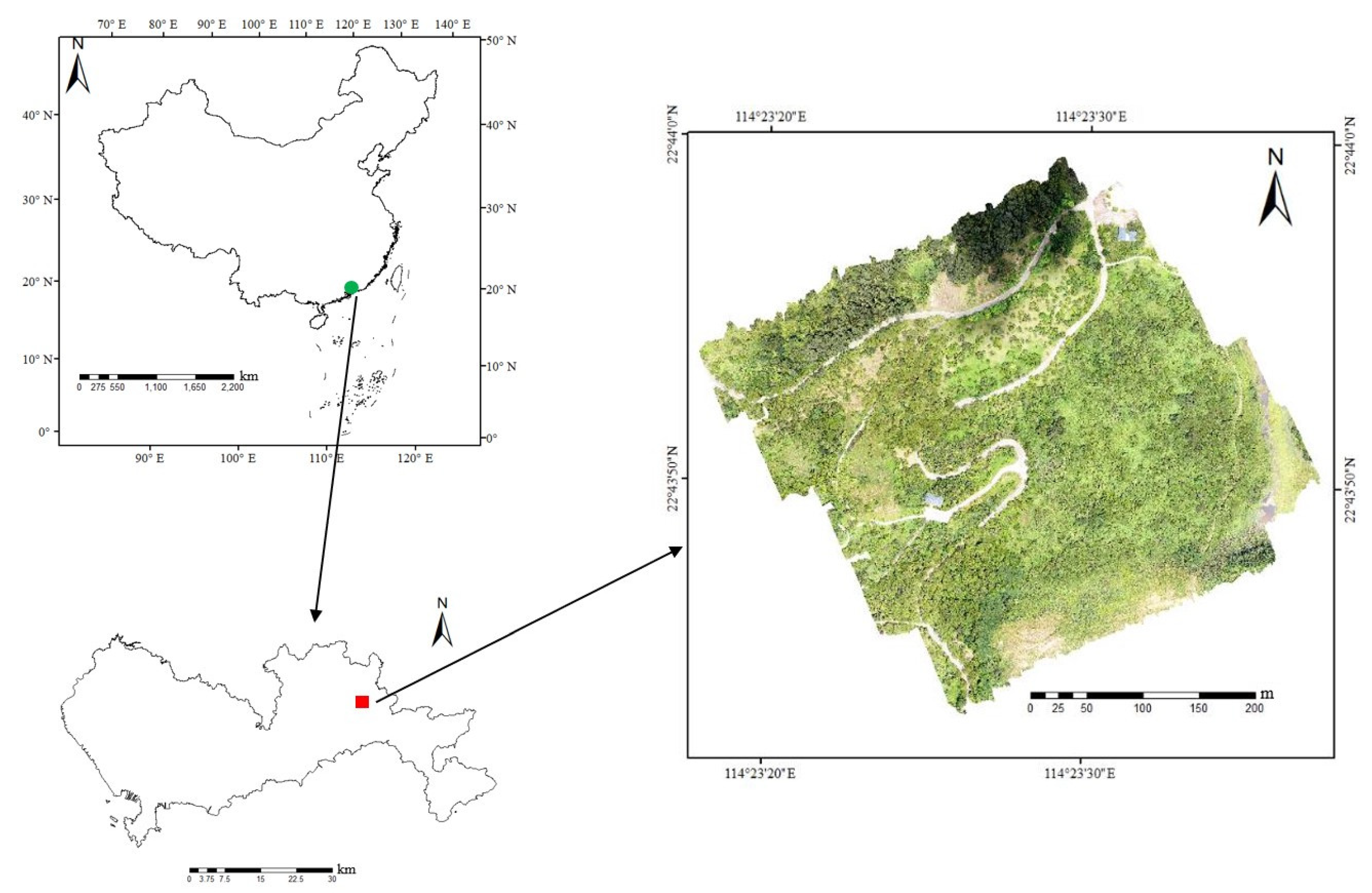
2.1. Study Area

The study area is located on Julongshan Park, a subtropical broadleaf forest situated in Shenzhen in southern China (Figure 1). The center coordinates of the study region are 114°23′28″E and 22°43′50″N. The topography of the study region is plain, with a mean altitude of 64 m. The climate is subtropical maritime, with an annual average temperature of 22.4 °C and an annual rainfall of 1933.3 mm. There are several tree species in the study area, such as Terminalia mantaly, Elaeocarpus grandifloras, Litchi chinensis, Lagerstroemia speciosa, Acacia mangium, and Cinnamomum camphora. Due to the limitations of field accessibility and sample number, this research was only conducted on Terminalia mantaly which accounted for about 50% of total individuals.

2.2. Remote Sensing Data

2.2.1. LiDAR Data

The LiDAR data were acquired on August 2019, by a Velodyne LiDAR PUCK-16 laser mounted on the DJI Matrice 600 Pro six-rotor aircraft (DJI, Shenzhen, China). The laser emitted pulse at a frequency of 5 kHz with a wavelength of 903 nm. The flight altitude was about 70 m above ground and the average flying speed was 3.6 m/s. Two returns were recorded for each pulse, and the average point cloud density was larger than 100 points/m². The point clouds were first filtered into ground points and nonground points by the TerraSolid software (Terrasolid, Helsinki, Finland). The density of the final point cloud containing only ground-level observations was 8 points/m². TerraSolid software uses an adaptive TIN algorithm for filtering, which was first proposed by Axelsson et al. [39] Next, digital terrain model (DTM) and digital surface model (DSM) were produced based on ground points and all points, respectively. Then, a canopy height model (CHM), representing the height of the vegetation above ground surface, was calculated by subtracting DTM values from DSM values. Finally, z-values of points were normalized by subtracting DTM values from the initial, absolute, z-values [40].

2.2.2. Hyperspectral Data

UAV hyperspectral imagery were acquired on August 2019 by the DJI Matrice 600 Pro UAV with a Resonon Pika-L sensor, which is a push-broom hyperspectral sensor. The hyperspectral images had 150 spectral bands between 400 nm and 1000 nm, with a spectral resolution of 2.2 nm. The flight altitude was about 200 m above ground, obtaining the hyperspectral images with a spatial resolution of 0.3 m. The hyperspectral images were first radiometrically corrected according to reference data, then geometrical corrections were carried out based on LiDAR-derived DTM and ground-based GPS data. Finally, atmospheric corrections were applied using the FLAASH module of ENVI software.

2.3. Field Data

A fieldwork campaign was carried out in August 2019. A total number of 60 Terminalia mantaly trees were measured. The tree height (H) and DBH were measured using a laser hypsometer and a tape measure respectively, and the position of each tree was acquired using a real-time kinematic GPS (RTK-GPS). Based on the carbon coefficient (CC) and aboveground biomass (AGB), tree-level carbon stock (CS) was calculated to serve as control data (Equation (1)) [15]. After an in-depth literature analysis, no available carbon coefficient and allometric growth equation for Terminalia mantaly have yet been discovered. Thus, since this species is a subtropical deciduous broad-leaved tree species in China, we decided instead to use the general carbon coefficient and allometric growth equation of subtropical deciduous broad-leaved forest from China. The allometric growth equation and carbon coefficient were obtained by cutting down trees, then drying, burning, and weighing them, and finally, we performed a regression analysis. In this study, the carbon coefficient of Terminalia mantaly was set to 0.4956 according to Li et al. [41] The aboveground biomass of each individual tree was calculated as the sum of different forest components, including stem biomass (stemAGB), branch biomass (branchAGB), and leaf biomass (leafAGB) (Equation (2)) [42]. The biomass of stem, branch, and leaf were calculated based on their DBH and height according to the allometric growth equation as shown in Equations (3)–(5), whose reported r² values are 0.98, 0.97, and 0.96, respectively [42].

$$CS=AGB\times CC$$

(1)

$$AGB=stemAGB+branchAGB+leafAGB$$

(2)

$$stemAGB=0.0263\times {(DB{H}^{2}H)}^{0.9695}$$

(3)

$$branchAGB=0.0232\times {(DB{H}^{2}H)}^{0.8055}$$

(4)

$$leafAGB=0.0075\times {(DB{H}^{2}H)}^{0.8015}$$

(5)

3. Methods

Tree-level carbon stocks were estimated by UAV LiDAR and hyperspectral data. The procedure consisted of three main steps: (1) individual tree segmentation; (2) tree-level structure and spectral features extraction; and (3) tree-level carbon stocks estimation (Figure 2).

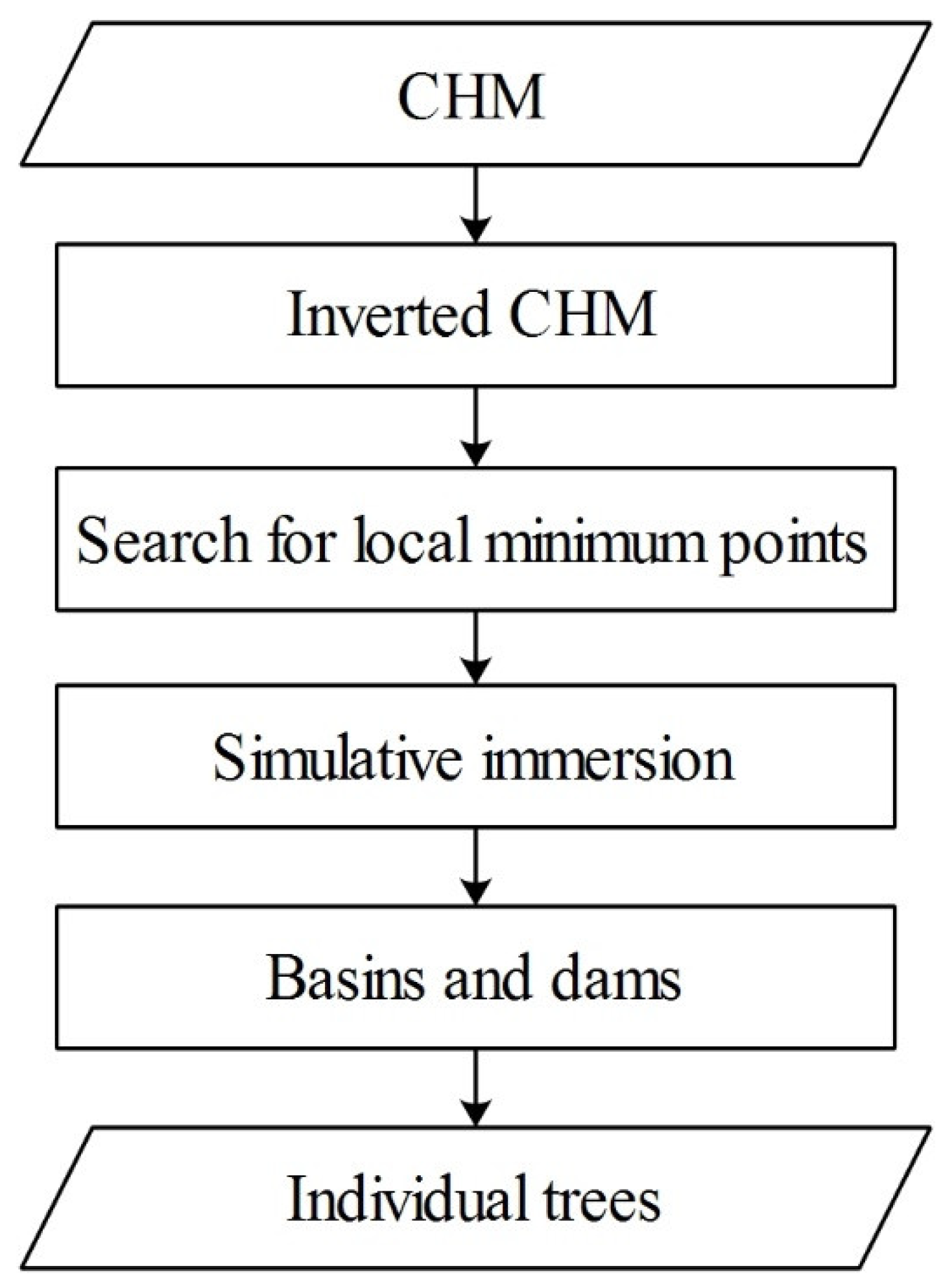
3.1. Individual Tree Segmentation

In this study, a CHM-based watershed segmentation algorithm was used to delineate tree crowns, which had been successfully used for individual tree segmentation in many studies [43,44,45,46,47,48]. The procedure of CHM-based watershed segmentation (Figure 3) is presented in detail by Chen et al. [44]. Initially, we subtracted CHM from its maximum value to obtain the inverted CHM. Next, a local minimum filter algorithm was used to find local minimum points from the inverted CHM. Then, these local minimum points were used as markers to simulate the immersion process. The influence area of each local minimum point expanded outward gradually, and “dams” were built at the confluence of multiple “basins”, which formed a “watershed”. Finally, the CHM was segmented to obtain individual trees.

3.2. LiDAR Features Extraction

To estimate tree-level carbon stocks, we extracted 10 structural features from UAV LiDAR data, including tree height, crown width, and the distribution characteristics of point clouds, which have been commonly used in forest aboveground biomass and carbon stocks estimation [26,49,50,51]. LiDAR features and their formulas are shown in

Table 1. List of LiDAR features.

Features	Formula/Description
Tree height	$H=\max \left(h_i\right)$
Crown diameter	$\mathrm{CD}=\frac{C{D}_{S\_N}+C{D}_{E\_W}}{2}$
Hmean	$H_{mean}=\frac{{\sum }_1^n{h}_i}{n}$
PH10	$\mathrm{The} 10\mathrm{th} \mathrm{height} \mathrm{percentile} \mathrm{of} \mathrm{point}$ clouds
PH25	$\mathrm{The} 25\mathrm{th} \mathrm{height} \mathrm{percentile} \mathrm{of} \mathrm{point}$ clouds
PH50	The 50th height percentile of point clouds
PH75	The 75th height percentile of point clouds
PH90	The 90th height percentile of point clouds
PH95	The 95th height percentile of point clouds
Hstd	${\mathrm{H}}_{\mathrm{s}\mathrm{t}\mathrm{d}}=\sqrt{\frac{\sum (H_i-H_{mean})}{n}}$

. LiDAR features extraction was implemented by programming with Matlab software.

Where CD_{S_N} and CD_{E_W} are the crown diameters in south–north direction and east–west direction, respectively. h_i is the height of the ith point, and n is the number of LiDAR points.

3.3. Hyperspectral Features Extraction

Nineteen tree-level narrowband spectral features, which are commonly used in forest carbon stocks or biomass estimation, were extracted from hyperspectral imagery, including principal components, band reflectance, and vegetation indices, to estimate carbon stock. The first three principal components were extracted by principal component analysis (PCA) algorithm. The mean vegetation indices and band reflectance of each tree were calculated based on hyperspectral data. Hyperspectral features and their formulas are shown in

Table 2. List of hyperspectral features.

Features	Formula	Reference
Enhanced vegetation index	$EVI=2.5\times \frac{{\rho }_{798}-{\rho }_{679}}{1+{\rho }_{798}+6\times {\rho }_{679}-7.5\times {\rho }_{482}}$	Huete et al., 2002 [52]
Mean red edge	${\mathrm{Mean}}_{690-740}=\frac{{{\displaystyle \sum }}_{690}^{740}{\rho }_i}{n}$	Coops et al., 2001 [53]
Adjusted vegetation index	$\mathrm{SAVI}=1.5\times \frac{{\rho }_{798}-{\rho }_{679}}{{\rho }_{798}-{\rho }_{679}+0.5}$	Jiang et al., 2007 [54]
Red edge ratio vegetation index	$\mathrm{MRESRI}=\frac{{\rho }_{750}-{\rho }_{445}}{{\rho }_{750}+{\rho }_{445}}$	Ballester et al., 2019 [55]
Datt Chlorophyll content index	$Datt=\frac{{\rho }_{850}-{\rho }_{710}}{{\rho }_{850}-{\rho }_{680}}$	Datt et al., 1999 [56]
Plant pigment ratio	$PPR=\frac{{\rho }_{550}-{\rho }_{450}}{{\rho }_{550}+{\rho }_{450}}$	Wang et al., 2004 [57]
Plant senescence reflectance index	$PSRI=\frac{{\rho }_{695}}{{\rho }_{760}}$	Carter et al., 1994 [58]
Structurally insensitive pigment index	$SIPI=\frac{{\rho }_{800}-{\rho }_{450}}{{\rho }_{800}+{\rho }_{680}}$	Zarco-Tejada et al., 2005 [59]
Photochemical reflectance index	$PRI=\frac{{\rho }_{570}-{\rho }_{530}}{{\rho }_{570}+{\rho }_{530}}$	Gamon et al., 1995 [60]
Modified normalized differential vegetation index	$MNDVI=\frac{{\rho }_{750}-{\rho }_{705}}{{\rho }_{750}+{\rho }_{705}-{\rho }_{445}\times 2}-1$	Rouse et al., 1974 [61]
Vogelmann red edge index	$VOG=\frac{{\rho }_{740}}{{\rho }_{720}}$	Vogelmann et al., 1993 [62]
Green index	$GI=\frac{{\rho }_{798}}{{\rho }_{553}}-1$	Zarco-Tejada et al., 2005 [59]
Anthocyanin content index	$ACI=\frac{{\rho }_{650}}{{\rho }_{550}}$	Sims et al., 2002 [63]
Slope of red edge	$SL=\frac{{\rho }_{740}-{\rho }_{690}}{50}$	Coops et al., 2001 [53]
Band value of 550nm	${\rho }_{550}$	Haboudane et al., 2004 [64]
Band value of 750nm	${\rho }_{750}$	Haboudane et al., 2004 [64]
1st principal component	$PCA1$
2nd principal component	$PCA2$
3rd principal component	$PCA3$

. Hyperspectral features extraction was implemented using ENVI software.

Where ${\rho }_{\mathrm{wavelength}}$ means the reflectance in the wavelength. For example, ${\rho }_{798}$ means the reflectance in the wavelength of 798 nm. n means the number of bands.

3.4. Tree-Level Carbon Stock Estimation

Pearson correlation analysis was carried out to explore the relationship between LiDAR features, hyperspectral features, and control data. Pearson correlation analysis was implemented using IBM SPSS Statistics 22 software. The LiDAR and hyperspectral features having a significant correlation with control data (with an absolute value of correlation coefficient (r) greater than 0.5) were selected for subsequent carbon stocks estimation of individual trees. The tree-level carbon stock estimation model has the form of the Schumacher–Hall formula as expressed in Equation (6), where LI_i refers to the ith LiDAR-derived structural feature, SI_j refers to the jth narrowband hyperspectral feature, c, a_i, and b_j are the regression coefficients. In order to facilitate modeling, the natural logarithm transformation of model (6) was carried out to obtain the model form (Equation (7)).

$$CS=c\times {\displaystyle \prod _{i=1}^{n}L{I}_i^{a_i}}\times {\displaystyle \prod _{j=1}^{m}S{I}_j^{b_j}}$$

(6)

$$\ln CS=\ln c+{\displaystyle \sum _{i=1}^n{a}_i\ln L{I}_i+{\displaystyle \sum _{j=1}^m{b}_j\ln S{I}_j}}$$

(7)

To investigate which combination of LiDAR and hyperspectral features can best explain the variance of tree-level carbon stocks, a stepwise multiple regression analysis was carried out. Stepwise multiple regression was implemented using IBM SPSS Statistics 22 software. Stepwise multiple regression is a commonly-used and effective method to eliminate the multicollinearity issue and select the optimal regression equation, which has been widely used to estimate forest carbon stocks or biomass [65,66]. To estimate carbon stocks of individual trees accurately, stepwise multiple regression models, which included LiDAR metrics and hyperspectral metrics as predictors, were developed independently and in combination.

3.5. Accuracy Assessment

To assess the predictive performance of tree-level carbon stock estimation models, five accuracy assessment measures were applied. The coefficient of determination (r²) (Equation (8)), root mean square error (RMSE) (Equation (9)), and mean absolute error (MAE) (Equation (10)) have been widely used to evaluate the prediction accuracy [26]. Percentage RMSE (PRMSE) is RMSE expressed as a percentage of the mean value (Equation (11)). Root mean square percentage error (RMSPE) is an average deviation from a true value (Equation (12)). PRMSE and RMSPE are all scale-independent metrics to assess the predictive performance of a model. In Equations (8)—(12), n is the number of samples, $y_i$ and ${\widehat{y}}_i$ are the true and predicted values of the ith sample, and $\overline{y}$ is the average true value of all samples. In this study, MAE, RMSE, PRMSE, and RMSPE were used to evaluate the prediction accuracy of tree-level carbon stock estimation models, and the model with a smaller metric value was considered to have a higher tree-level carbon stock accuracy. The overall prediction performance (OPP) of tree-level carbon stock estimation model can be calculated according to Equation (13). The model’s uncertainty can be calculated according to Equation (14). Lower values for Uncertainty increase the reliability of predictions. These accuracy metrics were calculated by programming with Matlab software.

$$r^2=\frac{{\displaystyle \sum _{i=1}^n{(\widehat{y}-\overline{y})}^2}}{{\displaystyle \sum _{i=1}^n{(y-\overline{y})}^2}}$$

(8)

$$RMSE=\sqrt{\frac{1}{n}{\displaystyle \sum _{i=1}^n{({\widehat{y}}_i-y_i)}^2}}$$

(9)

$$MAE=\frac{1}{n}\left[{\displaystyle \sum _{i=1}^{n}abs({\widehat{y}}_i-y_i)}\right]$$

(10)

$$PRMSE=(\frac{RMSE}{\overline{y}})\times 100\%$$

(11)

$$RMSPE=(\sqrt{\frac{1}{n}{\displaystyle \sum _{i=1}^n{(\frac{{\widehat{y}}_i-y_i}{y_i})}^2}})\times 100\%$$

(12)

$$OPP=100-\frac{PRMSE+RMSPE}{2}$$

(13)

$$Uncertainty=r^2-OPP$$

(14)

4. Results

Pearson correlation analysis was carried out to explore the relationship between each remote sensing feature and control data. The correlation coefficients between LiDAR features, hyperspectral features, and control data are plotted in Figure 4. Nine of the ten LiDAR features, including crown width, tree height, H_mean, the height percentiles of point clouds, had positive correlations with control data. All of the above had correlation coefficients larger than 0.48. Only one LiDAR feature, i.e., H_std, had no correlation with control data. For all the LiDAR features, tree height had the highest correlation with control data (r = 0.75), followed by PH95 (r = 0.70) and PH90 (r = 0.68). Among the 19 hyperspectral features, six features (PCA3, Datt, GI, mNDVI, VOG, and MRESRI) had positive correlations greater than 0.5 with control data, and four features (PCA2, ACI, PSRI, and SIPI) had negative correlations lower than -0.3 with control data. For all hyperspectral features, GI had the highest correlation with control data (r = 0.83), followed by VOG (r = 0.75) and MRESRI (r = 0.75).

As shown in

Table 3. Tree-level carbon stock estimation models using LiDAR and hyperspectral features.

Data Sources	Model ID	Formula (kg Per Tree)	r2
LiDAR	L1	$CS=0.37\times H^{1.90}$	0.66
	L2	$CS=0.48\times H^{1.70}\times PH{10}^{0.13}$	0.70
	L3	$CS=0.32\times H^{2.68}\times PH{10}^{0.22}\times H_{mean}{}^{-0.99}$	0.74
Hyperspectral	H1	$CS=0.35\times G{I}^{2.99}$	0.72
	H2	$CS=0.94\times G{I}^{2.59}\times mNDV{I}^{1.01}$	0.75
$\mathrm{LiDAR}+\mathrm{Hyperspectral}$	LH1	$CS=0.35\times G{I}^{2.99}$	0.72
	LH2	$CS=0.12\times G{I}^{2.29}\times PH{95}^{0.96}$	0.89

, the tree-level carbon stock models derived from LiDAR metrics alone, hyperspectral metrics alone, and the combination of them were coded with “L”, “H”, and “LH”, respectively. These models were derived by multiple stepwise regression. Among the ten LiDAR metrics, tree height, 10th height percentile of point clouds, and mean point height were selected by stepwise regression to develop the tree-level carbon stock estimation model. From all hyperspectral metrics, GI and mNDVI were selected to establish the tree-level carbon stock estimation model. When combining LiDAR and hyperspectral metrics, the tree-level carbon stock estimation model was established based on GI and 10th height percentile of point clouds.

The coefficient of determination (r²) of those tree-level carbon stock estimation models ranged from 0.66 to 0.89. Among the three kinds of tree-level carbon stock models, the LiDAR-derived model had the smallest r², where the r² values of model L1, L2, and L3 were 0.66, 0.70, and 0.74, respectively. The hyperspectral-derived model had a higher r² than the LiDAR-derived model, in which the r² values of model H1 and H2 were 0.72 and 0.75, respectively. The combined model (GI and PH95 are the predictors) had the highest r² (0.89).

Beyond the coefficient of determination, four accuracy statistical indices, MAE, RMSE, PRMSE, and RMSPE, were calculated to evaluate the bias of tree-level carbon stock estimation models. As shown in Figure 5, the MAE of the four models ranged from 2.36 kg to 5.86 kg with an average value of 4.55 kg. The RMSE ranged from 3.98 kg to 8.21 kg with an average of 6.56 kg. The PRMSE ranged from 14% to 30% with an average of 23%. The RMSPE ranged from 15% to 30% with an average of 24%. Among the three kinds of tree-level optimal carbon stock estimation models, the combined model (LH2) had the lowest bias, with a MAE of 2.36 kg, RMSE of 3.98 kg, PRMSE of 14%, and RMSPE of 22%. The bias of hyperspectral-derived optimal model (H2) was in the middle, with MAE of 4.08 kg, RMSE of 5.76 kg, PRMSE of 21%, and RMSPE of 22%. The LiDAR-derived optimal model (L3) had the highest bias, with MAE of 5.24 kg, RMSE of 7.42 kg, PRMSE of 27%, and RMSPE of 23%.

As shown in Figure 6, the control data ranged from 5.98 kg to 56.28 kg with an average of 27.71 ± 11.30 kg. LiDAR-derived models had slightly smaller mean and standard deviation than control data, and the maximum value and the minimum value were all higher than control data. Hyperspectral-derived models also had slightly smaller mean and standard deviation, and their ranges of maximum and minimum values were significantly smaller than control data. The minimum value, maximum value, range, and average value of the combined model were all closest to control data. Therefore, the combined model had the optimal tree-level carbon stock estimation results.

The overall prediction performance and uncertainty of all models are shown in

Table 4. A comparison of models’ overall prediction performance and uncertainty.

Model ID	L1	L2	L3	H1	H2	LH1	LH2
r2	66	70	74	72	75	72	89
OPP	70	73	75	77	79	77	85
Uncertainty	−4	−3	−1	−5	−4	−5	−4

. The values of OPP of all models ranged from 70 to 85. The uncertainties of all models ranged from −5 to −1. The OPP and uncertainty of these models are similar, so these models can account for variations in tree-level carbon stocks.

5. Discussion

Among all LiDAR-derived structural features, tree height showed the highest correlation with tree-level carbon stocks. This is an indication that tree height is the dominant factor of carbon stock estimation, which is consistent with previous studies [67,68]. The point height distribution features, including PH95, PH90, H_mean, PH75, PH50, PH25, and PH10, are also correlated well with carbon stock. This is because these features can describe the vertical structure of forest, which have an influence on carbon stock [68]. Crown diameter had weak correlation with carbon stock (r = 0.48), and no correlation was found between H_std and carbon stock. Additionally, stepwise multiple regression results indicated that the combination of tree height, PH10, and H_mean could provide accurate carbon stock estimation of individual trees. This may be owing to the fact that carbon stock is mainly determined by tree height and vertical structure [68,69].

Previous studies have found that hyperspectral metrics can be used to estimate forest aboveground biomass at plot level [36,70,71]. Luo et al. estimated plot-level forest biomass using hyperspectral-derived narrow-band vegetation indices, and the estimated biomass showed a good correlation with field biomass [72]. Gong et al. used airborne hyperspectral imagery to estimate forest biomass, and they found vegetation indices and red edge positions were effective for forest biomass retrieval [73]. This can be explained by the fact that hyperspectral data could describe the forest growth status, which is related to biomass [36,70]. However, our approach, in contrast to previously cited research, was to explore the ability of hyperspectral features in estimating tree-level carbon stock. For hyperspectral metrics, GI was most relevant to tree-level carbon stock as it explained 72% of the variance of carbon stocks. The absolute correlation coefficient between calculated carbon stock and PCA2, PCA3, Datt, PSRI, VOG, and MRESRI were all greater than 0.5. These results indicated that hyperspectral features had potential in estimating tree-level carbon stock.

Stepwise multiple regression showed that the combined model provided the highest tree-level carbon stock estimation accuracy. In addition, the predictions of the combined model were closest to control data. Therefore, combining UAV LiDAR and hyperspectral features could improve the accuracy of tree-level carbon stock estimation than using LiDAR and hyperspectral data alone. The improvement might be due to the complementarity between LiDAR-detected structural characteristics and hyperspectral-captured vegetation spectral information, and the combined model took full advantage of the predictive ability of structural features and hyperspectral features, which is consistent with previous studies [72,74,75]. Several studies have combined hyperspectral and LiDAR data to estimate carbon stocks at individual tree level [34,76,77]. They used hyperspectral information to classify tree species, and then developed carbon stock estimation model based on LiDAR-derived structural features. Kandare et al. [38] classified tree species using hyperspectral data and estimated broadleaf tree-level volume using LiDAR-derived tree height and DBH, resulting in an estimation accuracy of 58%. Alonzo et al. [74] estimated tree-level carbon stocks of a broadleaf tree species (e.g., Quercus agrifolia) by 28 LiDAR-derived structural metrics, with an accuracy of 83%. In this study, hyperspectral features and LiDAR structural features were combined to develop tree-level carbon stock estimation model, and they explained 89% of the variance in tree-level carbon stock. The higher estimation accuracy of tree-level carbon stocks reported in our study owes to the introduction of hyperspectral features. This can be explained by the fact that carbon stock is not only related to tree-level structural features that can be extracted from LiDAR data, but also to biomass conversion factor and carbon coefficient which can be reflected in hyperspectral information [37].

6. Conclusions

In this study, we explored the ability of combining UAV LiDAR and hyperspectral data in estimating tree-level carbon stocks in subtropical forests. We extracted tree-level structural and spectral features from UAV LiDAR and hyperspectral data, respectively, and then evaluated the capacities of LiDAR and hyperspectral features alone and in combination to predict aboveground carbon stock of individual trees. Results indicated that LiDAR or hyperspectral features alone can yield reasonable carbon stock (r² = 0.74 and 0.75, respectively). As expected, the combination of LiDAR and hyperspectral data could improve the accuracy of tree-level carbon stock estimation to some degree (r² = 0.89), and LiDAR-derived PH95 and hyperspectral-derived GI were included in the combination model. The improvement can be attributed to the fact that carbon stock is not only related to tree-level structural features that can be extracted from LiDAR data, but also to biomass conversion factor and carbon coefficient which can be reflected in hyperspectral information. Therefore, if both LiDAR and hyperspectral data are available, the fusion of LiDAR and hyperspectral data is the best method to accurately estimate tree-level aboveground carbon stock. This study could be a valuable resource for researchers and forest managers to obtain more accurate tree-level carbon stocks. Further efforts should focus on improving this approach or applying it to more forest types that have specific allometric equations, as well as in larger areas. In addition, based on the method of tree-level carbon stock estimation, multi-temporal remote sensing data should be obtained and then used to estimate forest carbon sequestration to ameliorate the unavoidable impacts of climate change.

References

1. Mitchard, E.T.A. The tropical forest carbon cycle and climate change. Nature 2018, 559, 527–534. [Google Scholar] [CrossRef] [PubMed]
2. Brinck, K.; Fischer, R.; Groeneveld, J.; Lehmann, S.; Dantas de Paula, M.; Putz, S.; Sexton, J.O.; Song, D.; Huth, A. High resolution analysis of tropical forest fragmentation and its impact on the global carbon cycle. Nat. Commun. 2017, 8, 14855. [Google Scholar] [CrossRef] [Green Version]
3. Zhu, X.J.; Zhang, H.Q.; Gao, Y.N.; Yin, H.; Chen, Z.; Zhao, T.H. Assessing the regional carbon sink with its forming processes—A case study of Liaoning province, China. Sci. Rep. 2018, 8, 15161. [Google Scholar] [CrossRef] [Green Version]
4. Zhu, K.; Zhang, J.; Niu, S.; Chu, C.; Luo, Y. Limits to growth of forest biomass carbon sink under climate change. Nat. Commun. 2018, 9, 2709. [Google Scholar] [CrossRef] [Green Version]
5. Fang, J.; Yu, G.; Liu, L.; Hu, S.; Chapin, F.S., 3rd. Climate change, human impacts, and carbon sequestration in China. Proc. Natl. Acad. Sci. USA 2018, 115, 4015–4020. [Google Scholar] [CrossRef] [Green Version]
6. Csillik, O.; Kumar, P.; Mascaro, J.; O’Shea, T.; Asner, G.P. Monitoring tropical forest carbon stocks and emissions using Planet satellite data. Sci. Rep. 2019, 9, 17831. [Google Scholar] [CrossRef] [Green Version]
7. Cook-Patton, S.C.; Leavitt, S.M.; Gibbs, D.; Harris, N.L.; Lister, K.; Anderson-Teixeira, K.J.; Briggs, R.D.; Chazdon, R.L.; Crowther, T.W.; Ellis, P.W.; et al. Mapping carbon accumulation potential from global natural forest regrowth. Nature 2020, 585, 545–550. [Google Scholar] [CrossRef]
8. Lorenz, K.; Lal, R. Carbon Sequestration in Forest Ecosystems; Springer: Dordrecht, The Netherlands, 2010. [Google Scholar]
9. Dixon, R.K.K.; Solomon, A.; Brown, S.; Houghton, R.; Trexier, M.; Wisniewski, J. Carbon pools and flux of global forest ecosystems. Science 1994, 263, 185–190. [Google Scholar] [CrossRef] [PubMed]
10. IPCC. Fourth Assessment Report of the Intergovernmental Panel on Climate Change; IPCC: Geneva, Switzerland, 2007.
11. IPCC. Fifth Assessment Report of the Intergovernmental Panel on Climate Change; IPCC: Geneva, Switzerland, 2014.
12. García, M.; Riaño, D.; Chuvieco, E.; Danson, F.M. Estimating biomass carbon stocks for a Mediterranean forest in central Spain using LiDAR height and intensity data. Remote Sens. Environ. 2010, 114, 816–830. [Google Scholar] [CrossRef]
13. Gleason, C.J.; Im, J. A review of remote sensing of forest biomass and biofuel: Options for small-area applications. GISci. Remote Sens. 2011, 48, 141–170. [Google Scholar] [CrossRef]
14. Nilsson, M. Estimation of tree heights and stand volume using an airborne lidar system. Remote Sens. Environ. 1996, 56, 1–7. [Google Scholar] [CrossRef]
15. Liu, C.; Li, X. Carbon storage and sequestration by urban forests in Shenyang, China. Urban For. Urban Green. 2012, 11, 121–128. [Google Scholar] [CrossRef]
16. Escobedo, F.; Varela, S.; Zhao, M.; Wagner, J.E.; Zipperer, W. Analyzing the efficacy of subtropical urban forests in offsetting carbon emissions from cities. Environ. Sci. Policy 2010, 13, 362–372. [Google Scholar] [CrossRef]
17. Chen, J.M.; Liu, J.; Leblanc, S.G.; Lacaze, R.; Roujean, J.-L. Multi-angular optical remote sensing for assessing vegetation structure and carbon absorption. Remote Sens. Environ. 2003, 84, 516–525. [Google Scholar] [CrossRef]
18. Mckinley, D.C.; Ryan, M.G.; Birdsey, R.A.; Giardina, C.P.; Harmon, M.E.; Heath, L.S.; Houghton, R.A.; Jackson, R.B.; Morrison, J.F.; Murray, B.C.; et al. A synthesis of current knowledge on forests and carbon storage in the United States. Ecol. Appl. 2011, 21, 1902–1924. [Google Scholar] [CrossRef] [PubMed] [Green Version]
19. Tan, K.; Piao, S.L.; Peng, C.H.; Fang, J.Y. Satellite-based estimation of biomass carbon stocks for northeast China’s forests between 1982 and 1999. For. Ecol. Manag. 2007, 240, 114–121. [Google Scholar] [CrossRef]
20. Sun, Y.; Xie, S.; Zhao, S. Valuing urban green spaces in mitigating climate change: A city-wide estimate of aboveground carbon stored in urban green spaces of China’s Capital. Glob. Chang. Biol. 2019, 25, 1717–1732. [Google Scholar] [CrossRef] [PubMed]
21. Shen, G.; Wang, Z.; Liu, C.; Han, Y. Mapping aboveground biomass and carbon in Shanghai’s urban forest using Landsat ETM+ and inventory data. Urban For. Urban Green. 2020, 51, 126655. [Google Scholar] [CrossRef]
22. Swatantran, A.; Dubayah, R.; Roberts, D.; Hofton, M.; Blair, J.B. Mapping biomass and stress in the Sierra Nevada using lidar and hyperspectral data fusion. Remote Sens. Environ. 2011, 115, 2917–2930. [Google Scholar] [CrossRef] [Green Version]
23. Tsui, O.W.; Coops, N.C.; Wulder, M.A.; Marshall, P.L.; McCardle, A. Using multi-frequency radar and discrete-return LiDAR measurements to estimate above-ground biomass and biomass components in a coastal temperate forest. ISPRS J. Photogramm. Remote Sens. 2012, 69, 121–133. [Google Scholar] [CrossRef]
24. Lefsky, M.A.; Cohen, W.B.; Parker, G.G.; Harding, D.J. Lidar remote sensing for ecosystem studies. Bioscience 2002, 52, 19–30. [Google Scholar] [CrossRef]
25. Mallet, C.; Bretar, F. Full waveform topographic lidar: State-of-the-art. Trait. Signal 2007, 24, 385–409. [Google Scholar] [CrossRef]
26. Qin, H.; Wang, C.; Xi, X.; Tian, J.; Zhou, G. Estimation of coniferous forest aboveground biomass with aggregated airborne small-footprint LiDAR full-waveforms. Opt. Express 2017, 25, A851–A869. [Google Scholar] [CrossRef] [PubMed]
27. Wang, C. Space Technologies for Low Carbon Development:LIDAR Applications for Forest Biomass Mapping; Science Press: Xi’an, China, 2013; p. 1. [Google Scholar]
28. Lin, C.; Thomson, G.; Popescu, S. An IPCC-compliant technique for forest carbon stock assessment using airborne LiDAR-derived tree metrics and competition index. Remote Sens. 2016, 8, 528. [Google Scholar] [CrossRef] [Green Version]
29. Gülçin, D.; van den Bosch, C.C.K. Assessment of above-ground carbon storage by urban trees using LiDAR data: The case of a university campus. Forests 2021, 12, 62. [Google Scholar] [CrossRef]
30. Schreyer, J.; Tigges, J.; Lakes, T.; Churkina, G. Using airborne LiDAR and QuickBird data for modelling urban tree carbon storage and its distribution—A case study of Berlin. Remote Sens. 2014, 6, 10636–10655. [Google Scholar] [CrossRef] [Green Version]
31. Coomes, D.A.; Dalponte, M.; Jucker, T.; Asner, G.P.; Banin, L.F.; Burslem, D.F.R.P.; Lewis, S.L.; Nilus, R.; Phillips, O.L.; Phua, M.-H.; et al. Area-based vs tree-centric approaches to mapping forest carbon in Southeast Asian forests from airborne laser scanning data. Remote Sens. Environ. 2017, 194, 77–88. [Google Scholar] [CrossRef] [Green Version]
32. Dalponte, M.; Ørka, H.O.; Ene, L.T.; Gobakken, T.; Næsset, E. Tree crown delineation and tree species classification in boreal forests using hyperspectral and ALS data. Remote Sens. Environ. 2014, 140, 306–317. [Google Scholar] [CrossRef]
33. Dalponte, M.; Reyes, F.; Kandare, K.; Gianelle, D. Delineation of individual tree crowns from ALS and hyperspectral data: A comparison among four methods. Eur. J. Remote Sens. 2015, 48, 365–382. [Google Scholar] [CrossRef] [Green Version]
34. Dalponte, M.; Coomes, D.A. Tree-centric mapping of forest carbon density from airborne laser scanning and hyperspectral data. Methods Ecol. Evol. 2016, 7, 1236–1245. [Google Scholar] [CrossRef] [Green Version]
35. Eysn, L.; Hollaus, M.; Lindberg, E.; Berger, F.; Monnet, J.-M.; Dalponte, M.; Kobal, M.; Pellegrini, M.; Lingua, E.; Mongus, D.; et al. A benchmark of Lidar-based single tree detection methods using heterogeneous forest data from the Alpine space. Forests 2015, 6, 1721–1747. [Google Scholar] [CrossRef] [Green Version]
36. Man, Q.; Dong, P.; Guo, H.; Liu, G.; Shi, R. Light detection and ranging and hyperspectral data for estimation of forest biomass: A review. J. Appl. Remote Sens. 2014, 8, 081598. [Google Scholar] [CrossRef]
37. Laurin, V.G.; Chen, Q.; Lindsell, J.A.; Coomes, D.A.; Frate, F.D.; Guerriero, L.; Pirotti, F.; Valentini, R. Above ground biomass estimation in an African tropical forest with lidar and hyperspectral data. ISPRS J. Photogramm. Remote Sens. 2014, 89, 49–58. [Google Scholar] [CrossRef]
38. Kandare, K.; Dalponte, M.; Ørka, H.; Frizzera, L.; Næsset, E. Prediction of species-specific volume using different inventory approaches by fusing airborne laser scanning and hyperspectral data. Remote Sens. 2017, 9, 400. [Google Scholar] [CrossRef] [Green Version]
39. Axelsson, P. DEM generation from laser scanner data using adaptive TIN models. Int. Arch. Photogramm. Remote Sens. 2000, 33, 111–118. [Google Scholar]
40. Nie, S.; Wang, C.; Zeng, H.; Xi, X.; Li, G. Above-ground biomass estimation using airborne discrete-return and full-waveform LiDAR data in a coniferous forest. Ecol. Indic. 2017, 78, 221–228. [Google Scholar] [CrossRef]
41. Li, H. Estimation and Evaluation of Forest Biomass Carbon Storage in China; China Forestry Publishing House: Beijing, China, 2010. [Google Scholar]
42. Zhou, G.; Yin, G.; Tang, X.; Wen, D.; Liu, C.; Kuang, Y.; Wang, W. Carbon Storage of Forest Ecosystem in China—Biomass Equation; Science Press: Beijing, China, 2018. [Google Scholar]
43. Yang, J.; Kang, Z.; Cheng, S.; Yang, Z.; Akwensi, P.H. An individual tree segmentation method based on watershed algorithm and three-dimensional spatial distribution analysis from airborne LiDAR point clouds. IEEE J.-STARS 2020, 13, 1055–1067. [Google Scholar] [CrossRef]
44. Chen, Q.; Baldocchi, D.; Gong, P.; Kelly, M. Isolating individual trees in a Savanna woodland using small footprint lidar data. Photogramm. Eng. Remote Sens. 2006, 72, 723–732. [Google Scholar] [CrossRef] [Green Version]
45. Kim, S.R.; Kwak, D.A.; Lee, W.K.; Son, Y.; Bae, S.W.; Kim, C.; Yoo, S. Estimation of carbon storage based on individual tree detection in Pinus densiflora stands using a fusion of aerial photography and LiDAR data. Sci. China Life Sci. 2010, 53, 885–897. [Google Scholar] [CrossRef] [PubMed]
46. Alonzo, M.; Bookhagen, B.; Roberts, D.A. Urban tree species mapping using hyperspectral and lidar data fusion. Remote Sens. Environ. 2014, 148, 70–83. [Google Scholar] [CrossRef]
47. Kwak, D.A.; Lee, W.K.; Cho, H.K.; Lee, S.H.; Son, Y.; Kafatos, M.; Kim, S.R. Estimating stem volume and biomass of Pinus koraiensis using LiDAR data. J. Plant Res. 2010, 123, 421–432. [Google Scholar] [CrossRef]
48. Ganjee, R.; Moghaddam, M.E.; Nourinia, R. Automatic segmentation of abnormal capillary nonperfusion regions in optical coherence tomography angiography images using marker-controlled watershed algorithm. J. Biomed. Opt. 2018, 23, 1–16. [Google Scholar] [CrossRef] [PubMed]
49. Popescu, S.C.; Wynne, R.H.; Nelson, R.F. Measuring individual tree crown diameter with lidar and assessing its influence on estimating forest volume and biomass. Can. J. Remote Sens. 2003, 29, 564–577. [Google Scholar] [CrossRef]
50. Cao, L.; Coops, N.; Hermosilla, T.; Innes, J.; Dai, J.; She, G. Using small-footprint discrete and full-waveform airborne LiDAR metrics to estimate total biomass and biomass components in subtropical forests. Remote Sens. 2014, 6, 7110–7135. [Google Scholar] [CrossRef] [Green Version]
51. Kankare, V.; Vastaranta, M.; Holopainen, M.; Räty, M.; Yu, X.; Hyyppä, J.; Hyyppä, H.; Alho, P.; Viitala, R. Retrieval of forest aboveground biomass and stem volume with airborne scanning LiDAR. Remote Sens. 2013, 5, 2257–2274. [Google Scholar] [CrossRef] [Green Version]
52. Huete, A.; Didan, K.; Miura, T.; Rodriguez, E.P.; Gao, X.; Ferreira, L.G. Overview of the radiometric and biophysical performance of the MODIS vegetation indices. Remote Sens. Environ. 2002, 83, 195–213. [Google Scholar] [CrossRef]
53. Coops, N.C.; Stone, C.; Merton, R.; Chisholm, L. Assessing eucalypt foliar health with field-based spectra and high spatial resolution hyperspectral imagery. In Proceedings of the IEEE International Geoscience & Remote Sensing Symposium, Sydney, Australia, 9–13 July 2001; IEEE: Piscataway, NJ, USA, 2001; Volume 602, pp. 603–605. [Google Scholar]
54. Jiang, Z.; Huete, A.; Li, J.; Qi, J. Interpretation of the modified soil-adjusted vegetation index isolines in red-NIR reflectance space. J. Appl. Remote Sens. 2007, 1, 013503. [Google Scholar] [CrossRef] [Green Version]
55. Ballester, C.; Brinkhoff, J.; Quayle, W.C.; Hornbuckle, J. Monitoring the effects of water stress in cotton using the green red vegetation index and red edge ratio. Remote Sens. 2019, 11, 873. [Google Scholar] [CrossRef] [Green Version]
56. Datt, B. A new reflectance index for remote sensing of chlorophyll content in higher plants: Tests using Eucalyptus leaves. J. Plant Physiol. 1999, 154, 30–36. [Google Scholar] [CrossRef]
57. Wang, Z.J.; Wang, J.H.; Liu, L.Y.; Huang, W.J.; Zhao, C.J.; Wang, C.Z. Prediction of grain protein content in winter wheat (Triticum aestivum L.) using plant pigment ratio (PPR). Field Crops Res. 2004, 90, 311–321. [Google Scholar] [CrossRef]
58. Carter, G.A.; Miller, R.L. Early detection of plant stress by digital imaging within narrow stress-sensitive wavebands. Remote Sens. Environ. 1994, 50, 295–302. [Google Scholar] [CrossRef]
59. Zarcotejada, P.; Berjon, A.; Lopezlozano, R.; Miller, J.; Martin, P.; Cachorro, V.; Gonzalez, M.; Defrutos, A. Assessing vineyard condition with hyperspectral indices: Leaf and canopy reflectance simulation in a row-structured discontinuous canopy. Remote Sens. Environ. 2005, 99, 271–287. [Google Scholar] [CrossRef]
60. Gamon, J.; Roberts, D.; Green, R. Evaluation of the photochemical reflectance index in AVIRIS imagery. In Proceedings of the Summaries of the Fifth Annual JPL Airborne Earth Science Workshop, Pasadena, CA, USA, 23–26 January 1995; California Institute of Technology: Pasadena, CA, USA, 1995; Volume 1. [Google Scholar]
61. Rouse, J.; Haas, R.; Schell, J.; Deering, D. Monitoring vegetation systems in the Great plains with ERTS. NASA Spec. Publ. 1974, 351, 309. [Google Scholar]
62. Vogelmann, T. Plant tissue optics. Annu. Rev. Plant Biol. 1993, 44, 231–251. [Google Scholar] [CrossRef]
63. Sims, D.A.; Gamon, J.A. Relationships between leaf pigment content and spectral reflectance across a wide range of species, leaf structures and developmental stages. Remote Sens. Environ. 2002, 81, 337–354. [Google Scholar] [CrossRef]
64. Haboudane, D. Hyperspectral vegetation indices and novel algorithms for predicting green LAI of crop canopies: Modeling and validation in the context of precision agriculture. Remote Sens. Environ. 2004, 90, 337–352. [Google Scholar] [CrossRef]
65. Sheridan, R.; Popescu, S.; Gatziolis, D.; Morgan, C.; Ku, N.-W. Modeling forest aboveground biomass and volume using airborne LiDAR metrics and forest inventory and analysis data in the Pacific Northwest. Remote Sens. 2014, 7, 229–255. [Google Scholar] [CrossRef]
66. Pirotti, F.; Laurin, G.; Vettore, A.; Masiero, A.; Valentini, R. Small footprint full-waveform metrics contribution to the prediction of biomass in tropical forests. Remote Sens. 2014, 6, 9576–9599. [Google Scholar] [CrossRef] [Green Version]
67. Wang, C.; Nie, S.; Xi, X.; Luo, S.; Sun, X. Estimating the biomass of maize with hyperspectral and LiDAR data. Remote Sens. 2016, 9, 11. [Google Scholar] [CrossRef] [Green Version]
68. Clark, M.L.; Roberts, D.A.; Ewel, J.J.; Clark, D.B. Estimation of tropical rain forest aboveground biomass with small-footprint lidar and hyperspectral sensors. Remote Sens. Environ. 2011, 115, 2931–2942. [Google Scholar] [CrossRef]
69. Latifi, H.; Fassnacht, F.; Koch, B. Forest structure modeling with combined airborne hyperspectral and LiDAR data. Remote Sens. Environ. 2012, 121, 10–25. [Google Scholar] [CrossRef]
70. Brovkina, O.; Novotny, J.; Cienciala, E.; Zemek, F.; Russ, R. Mapping forest aboveground biomass using airborne hyperspectral and LiDAR data in the mountainous conditions of Central Europe. Ecol. Eng. 2017, 100, 219–230. [Google Scholar] [CrossRef]
71. Koch, B. Status and future of laser scanning, synthetic aperture radar and hyperspectral remote sensing data for forest biomass assessment. ISPRS J. Photogramm. Remote Sens. 2010, 65, 581–590. [Google Scholar] [CrossRef]
72. Luo, S.; Wang, C.; Xi, X.; Pan, F.; Peng, D.; Zou, J.; Nie, S.; Qin, H. Fusion of airborne LiDAR data and hyperspectral imagery for aboveground and belowground forest biomass estimation. Ecol. Indic. 2017, 73, 378–387. [Google Scholar] [CrossRef]
73. Gong, B.; Im, J.; Jensen, J.R.; Coleman, M.; Rhee, J.; Nelson, E. Characterization of forest crops with a range of nutrient and water treatments using AISA hyperspectral imagery. GISci. Remote Sens. 2012, 49, 463–491. [Google Scholar] [CrossRef]
74. Alonzo, M.; McFadden, J.P.; Nowak, D.J.; Roberts, D.A. Mapping urban forest structure and function using hyperspectral imagery and lidar data. Urban For. Urban Green. 2016, 17, 135–147. [Google Scholar] [CrossRef] [Green Version]
75. Sarrazin, M.J.D.; van Aardt, J.A.N.; Asner, G.P.; McGlinchy, J.; Messinger, D.W.; Wu, J. Fusing small-footprint waveform LiDAR and hyperspectral data for canopy-level species classification and herbaceous biomass modeling in savanna ecosystems. Can. J. Remote Sens. 2014, 37, 653–665. [Google Scholar] [CrossRef]
76. Choudhury, M.A.M.; Marcheggiani, E.; Despini, F.; Costanzini, S.; Rossi, P.; Galli, A.; Teggi, S. Urban tree species identification and carbon stock mapping for urban green planning and management. Forests 2020, 11, 1226. [Google Scholar] [CrossRef]
77. Puliti, S.; Breidenbach, J.; Astrup, R. Estimation of forest growing stock volume with UAV laser scanning data: Can it be done without field data? Remote Sens. 2020, 12, 1245. [Google Scholar] [CrossRef] [Green Version]
Figure 1. Location of study area.
Remotesensing 13 04969 g001
Figure 2. The flowchart of tree-level carbon stocks estimation.
Remotesensing 13 04969 g002
Figure 3. The flowchart of CHM-based watershed segmentation.
Remotesensing 13 04969 g003
Figure 4. The correlation coefficients between LiDAR features, hyperspectral features, and control data.
Remotesensing 13 04969 g004
Figure 5. Prediction error and error percentage of tree-level carbon stock estimation models.
Remotesensing 13 04969 g005
Figure 6. The descriptive statistics of tree-level carbon stock of the observations and model estimates.
Remotesensing 13 04969 g006