Hybrids of Support Vector Regression with Grey Wolf Optimizer and Firefly Algorithm for Spatial Prediction of Landslide Susceptibility

Abstract

Landslides are one of the most frequent and important natural disasters in the world. The purpose of this study is to evaluate the landslide susceptibility in Zhenping County using a hybrid of support vector regression (SVR) with grey wolf optimizer (GWO) and firefly algorithm (FA) by frequency ratio (FR) preprocessed. Therefore, a landslide inventory composed of 140 landslides and 16 landslide conditioning factors is compiled as a landslide database. Among these landslides, 70% (98) landslides were randomly selected as the training dataset of the model, and the other landslides (42) were used to verify the model. The 16 landslide conditioning factors include elevation, slope, aspect, plan curvature, profile curvature, distance to faults, distance to rivers, distance to roads, sediment transport index (STI), stream power index (SPI), topographic wetness index (TWI), normalized difference vegetation index (NDVI), landslide, rainfall, soil and lithology. The conditioning factors selection and spatial correlation analysis were carried out by using the correlation attribute evaluation (CAE) method and the frequency ratio (FR) algorithm. The area under the receiver operating characteristic curve (AUROC) and kappa data of the training dataset and validation dataset are used to evaluate the prediction ability and the relationship between the advantages and disadvantages of landslide susceptibility maps. The results show that the SVR-GWO model (AUROC = 0.854) has the best performance in landslide spatial prediction, followed by the SVR-FA (AUROC = 0.838) and SVR models (AUROC = 0.818). The hybrid models of SVR-GWO and SVR-FA improve the performance of the single SVR model, and all three models have good prospects for regional-scale landslide spatial modeling.

1. Introduction

Landslide hazard refers to the geological process and natural phenomenon in which the rock and soil on the slope are affected by gravity and under the comprehensive influence of external factors [1,2]. The impact of social development and construction on the natural environment is self-evident. As the most serious geological disaster, the consequences and secondary disasters caused by landslide will not only cause serious harm to society, but also cause huge economic losses [3,4]. The prevention, control and treatment of landslide disasters brook no delay.

As the first step to prevent and control landslide disasters, landslide susceptibility mapping is a standard tool for land management decision-making to reduce landslide damage [5,6,7]. It classifies the areas prone to landslides, so as to formulate land management plans and decision-making schemes to reduce potential landslide disaster risks. Therefore, it can be considered that the landslide susceptibility map is an effective procedure to help humans identify and adapt to landslide disaster mitigation [8,9]. The mapping of landslide susceptibility mainly follows the following four parts: first, it is based on a landslide inventory map; second, it is necessary to create landslide conditioning factors directly or indirectly related to the landslide; then, qualitative or quantitative methods are used to estimate the correlation value between the landslide conditioning factors and the landslide; finally, the target area is divided into different types of landslide susceptible areas [10,11,12].

Up to now, many researchers have adopted several methods, including qualitative analysis and quantitative techniques, in order to improve the accuracy of landslide susceptibility mapping [8,13]. Three methods of landslide prediction and zoning based on GIS technology have been used many times, including heuristic, statistical and deterministic methods [8,14,15,16]. There are many traditional models, including: frequency ratio (FR) [17,18,19,20,21], certainty factor (CF) [22,23,24,25,26], weight of evidence (WoE) [27,28,29,30,31], fuzzy logic (FL) [32,33,34,35,36], analytic hierarchy process (AHP) [37,38,39,40], Dempster–Shafer (DS) [41,42,43,44,45], information value (IV) [46,47,48,49], and the geographic information system [50] matrix method [51,52]. Traditional models, like statistical models, are based on statistical assumptions and rely on a large number of datasets [53]. They no longer satisfy the modeling needs of researchers, and intelligent algorithms with higher precision have replaced traditional models, including: adaptive neuro-fuzzy inference system (ANFIS) [54,55,56,57], logistic regression (LR) [58,59,60,61,62], naive Bayes (NB) [63,64,65], kernel logistic regression (KLR) [66,67,68,69], decision tree (DT) [14,70,71,72,73,74], random forest (RF) [75,76,77,78,79], artificial neural network (ANN) [80,81,82,83,84], support vector machine (SVM) [14,85,86,87,88], generalized addition (GA) [89], general linear models (GLM) [90,91,92], and support vector regression (SVR) [53,93], as well as firefly algorithm (FA) [94] which can be used for optimization. Each model is different in data input process, operation calculation, data output process and predictive ability [95].

In recent years, the integrated modeling method of landslide susceptibility based on statistical models and the main research technology of machine learning algorithms has been recognized by many researchers, such as the combination of frequency ratio (FR) and logistic regression (LR) methods [8,96,97], the combination of bivariate statistical index and ANFIS [55], as well as the combination of physical model and convolutional neural network [98]. Two new hybrid integrated artificial intelligence models, LADT-bagging and FPA-bagging, are used to simulate the landslide susceptibility in the Youfanggou district [99]. It can be seen that these integrated models have stronger recognition ability and more accurate prediction ability. For this reason, more and more researchers are still exploring new integration technologies.

As a powerful geospatial evaluation model, the FR can assign probability weight to landslide conditioning factors, and its performance is stable and reliable. The SVR is a machine learning algorithm for regression analysis, which allows the prediction of continuous real valued variables. It can deal with nonlinear problems and high-dimensional data. The GWO and FA algorithm take the biological population relationship to seek the optimal solution as their respective principles. The GWO realizes the idealization of simulating the living habits of gray wolves in nature, and the FA realizes the idealization of firefly luminous characteristics. As meta-heuristic algorithms, both have good performance and are more suitable for spatial prediction.

In this article, three models (SVR, GWO, and FA) based on frequency ratio (FR) algorithm are proposed for spatial prediction of landslide susceptibility in Zhenping County, Shaanxi Province. This study aims to find the most suitable integrated modeling method for Zhenping County, and verify the overall effect of the hybrid model in landslide spatial prediction.

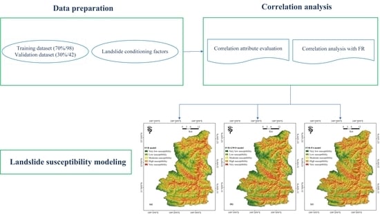
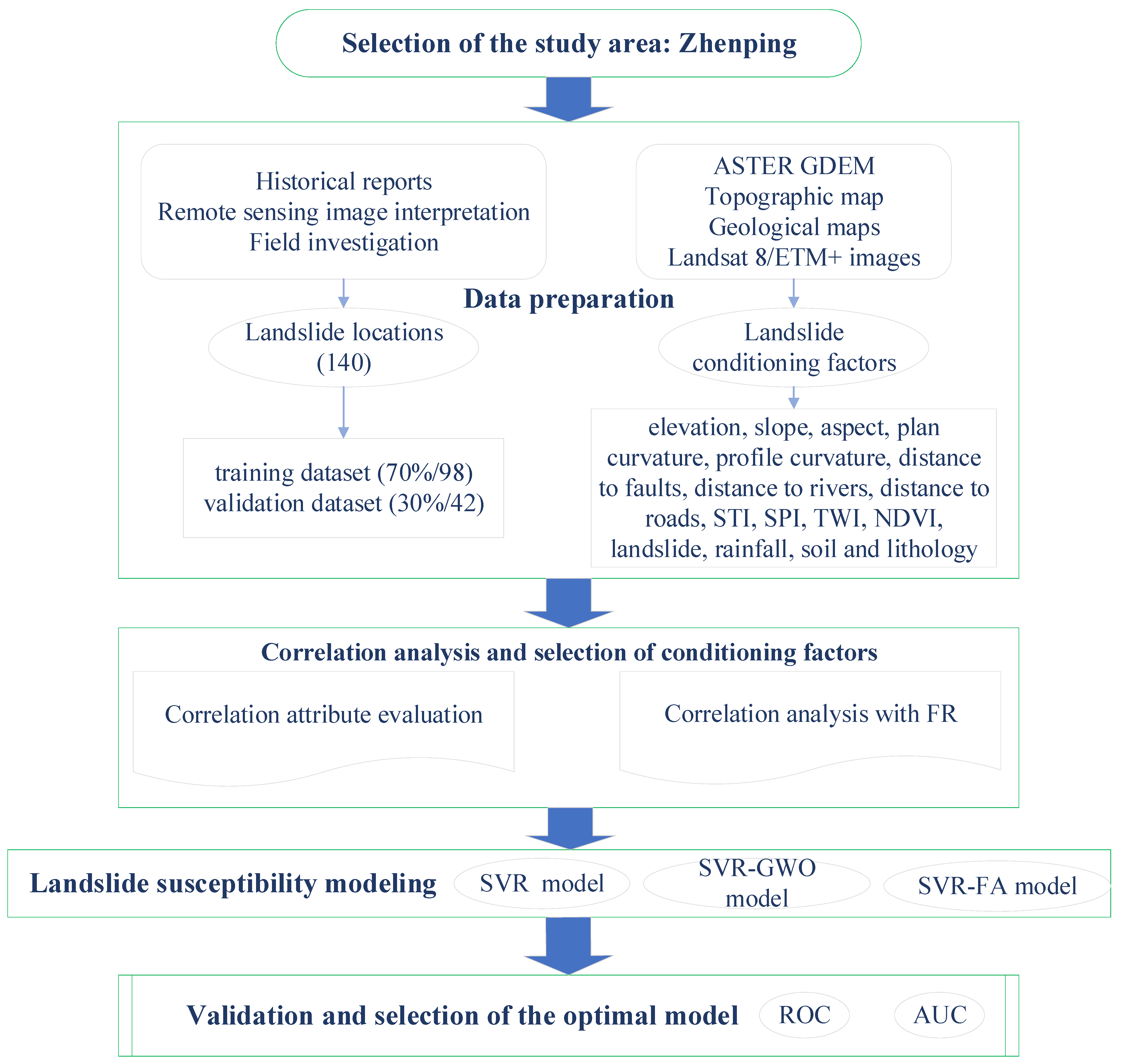
2. Study Area and Data Preparation

Zhenping County is located between longitudes 109°11′ E and 109°38′ E and between latitudes 31°42′ N and 32°13′ N, with an area of 1503.26 km² (Figure 1).

The southwest of Zhenping County lies on the main ridge of Daba Mountain, forming a terrain high in the southwest and low in the northeast. Most of the ridges along the southwestern mountains are about 2400 m above sea level. The ridges along the northeast mountains are between 1400 and 2500 m. The areas between 500 and 1000 m a.s.l. are distributed in the Nanjiang River and both banks of its tributaries. The relative height is large, and the slope is mostly between 20° and 45°. The areas between 1000 and 1500 m a.s.l. are characterized by a deep valley and a steep slope, and the relative height is 600–1000 m. The areas with altitudes higher than 1500 m include the main ridge of Daba Mountain and Hualong mountain. The main ridge mountains are obvious, the relative height is 600–1200 m, and the slope is mostly between 35° and 50°. This area is located in the Yangtze quasi-platform sedimentary area and the Qinling trough sedimentary area, and the stratigraphic lithology in the area is relatively complex.

The location of the previous landslide can be determined using a landslide inventory map containing landslide-related information [100]. The landslide data in this paper is based on the interpretation and extraction of high-resolution remote sensing images, historical reports and field survey, which are mostly developed in areas with strong human engineering activities such as towns, roads, and faults. There are 140 landslides in the study area, of which 119 are small-scale landslides, 20 medium-sized landslides and 1 large landslide. A total of 140 landslides were randomly divided into the training dataset and the testing dataset at a ratio of 7:3, which were converted into point features in GIS software with a resolution of 25 m.

According to the literature review, high-resolution remote sensing elevation data of the study area and geological and hydrological maps [3,10,101,102,103,104], 16 landslide hazard conditioning factors were analyzed and extracted, including topographic factors, geological factors, and environmental factors. The selected landslide conditioning factors include: elevation, slope, aspect, plan curvature, profile curvature, distance to faults, distance to rivers, distance to roads, sediment transport index (STI), stream power index (SPI), topographic wetness index (TWI), the normalized difference vegetation index (NDVI), land use, rainfall, soil and lithology. The 16 landslide conditioning factors are converted into a thematic data layer with a resolution of 25 m.

Elevation refers to the height of a point relative to the datum [105]. Many scholars use elevation to analyze the susceptibility of landslides [14]. It mainly affects slope stability through human engineering activities, vegetation distribution and land use types. In the GIS software, the elevation data is used to draw an elevation map with twelve categories (Figure 2a). The elevation of the study area is between 547–2911 m, most of which is enclosed between 1200–1800 m.

Slope refers to the angle between the slope surface and the horizontal direction, indicating the steepness of the slope, and is an important indicator that affects the stability of the slope [106,107]. The slope mainly affects the stress distribution state of the slope and is directly related to the sliding of the soil. GIS software was used to divide the slope into seven categories based on DEM data and draw a slope map (Figure 2b).

The aspect of the slope affects the amount of solar radiation received by the surface, which affects surface evaporation, weathering, vegetation coverage, and slope erosion, which in turn makes slope stability different [7,108]. In this paper, GIS software is used to divide the aspect into nine categories based on DEM data and draw the aspect map (Figure 2c). There is very little distribution of flat land in the study area, accounting for <0.01%, and the proportion of other slope directions > 10%, and the overall difference is small.

Plan curvature is an important factor in evaluating the vulnerability of landslides [109]. Plan curvature is a measure of the distortion of the ground surface in the horizontal direction, and describes the degree of curvature of the ground contour at the point [110]. In this study, a plan curvature map was drawn according to DEM (Figure 2d). According to the plan curvature, the slope can be divided into concave, plan and convex.

Profile curvature is a measure of the elevation change rate of the surface in the vertical direction, which describes the curvature and change of the ground in the slope direction [111]. Using DEM in GIS software, a profile curvature map was produced (Figure 2e). According to the profile curvature, the slope can be divided into concave, plan and convex.

Faults control the formation and development of geomorphology to a certain extent, and the degree of crustal stress, fracture and weathering are also affected by faults [112]. Using the fault map of the study area and the Euclidean distance analysis tool of the GIS software, the distance to faults map was extracted (Figure 2f).

The effect of surface water is that surface runoff erodes the river bank, makes the bank slope increase and steepen, erodes the slope toe, reduces the support force of the bank slope, and directly affects the saturation of the material to control stability [113]. The Euclidean distance analysis tool of the GIS software was used to extract the distance to rivers map (Figure 2g).

As one of the most important human factors influencing the occurrence of landslides, the construction of roads in the area must excavate the mountain because of the topographic constraints, and the roads affect the structure of the slope toe resulting in increased strain behind the slope and the development of cracks [114]. This is also the most important distribution feature of geological disasters in the region. The Euclidean distance analysis tool of the GIS software was used to extract the distance to roads map (Figure 2h).

STI characterizes erosion and deposition processes [20,115]. SPI shows the strength and erosion of slope runoff [116,117]. TWI describes the erosion and deposition process of the terrain [20]. In this paper, the GIS software is used to delineate these three factors (Figure 2i–k).

NDVI describes the vegetation coverage area and vegetation density in remote sensing images, and NDVI factors are indispensable in the prediction of landslide susceptibility [118]. The NDVI value of the study area was calculated according to the near-infrared and red bands of Landsat 8 OLI using the following formula (Figure 2l):

$$NDVI=(NIR-R)/(NIR+R)$$

(1)

where, R and NIR represent the infrared band (0.630–0.680 μm) and the near-infrared band (0.845–0.885 μm), respectively.

The unreasonable use of land by humans will destroy the stability of rock and soil and accelerate the occurrence of landslides. The paper analyzes the impact on landslides according to different types of land use [119]. In order to obtain an accurate description, the land use types are divided into six categories: farmland, forestland, grassland, water bodies, construction land, and bare land. Finally, a land use map is obtained (Figure 2m).

Rainfall is also an important factor for landslides. Because the study area is covered by a large area of loess, when soaked in water, their structure will become loose [120,121]. The GIS software was used to extract ten categories of rainfall map with an interval of 50 mm/yr (Figure 2n).

Different physical and mechanical properties of the soil affect surface water filtration and groundwater flow [122,123,124,125]. The soil map was developed based on the soil database by the Institute of Soil Science, Chinese Academy of Sciences. Using the GIS software, nine categories of the soil map was extracted (Figure 2o).

Lithology is the material basis for the development and occurrence of landslides. The weather resistance and strength of rocks and soil depend on the type of lithology [121]. On the other hand, the types and characteristics of landslides are different due to the combination of rock masses with different properties, hardness and structure [121]. This paper divides the lithology into ten types according to the geological ages and lithofacies (

Table 1. Description of the lithological units.

Group	Lithology	Geologic Ages
1	Trachyte	Silurian
2	Volcanic rock, diabase, diabase porphyrite	Silurian
3	Diabase	Palaeozoic
4	Metamorphic rhyolite, quartz porphyry, volcanic clastic rocks, phyllite, metamorphic sandstone	Proterozoic
5	Yellow-green and dark gray sandy slate, argillaceous slate, silty sericite phyllite, sandstone, siltstone, carbonaceous slate, tuff sandstone	Silurian
6	Slate, argillaceous limestone, banded slate, carbonaceous slate, silt sandstone, sandstone	Silurian
7	Gray-black siliceous rock, carbonaceous slate, yellow-green phyllite, schist, marl, limestone, calcareous slate, dolomite, breccia limestone	Cambrian
8	Dolomite, marl, shale, conglomerate, sandstone, limestone, carbonaceous slate	Ediacaran
9	Silty slate, siltstone, sandstone, tuff sandstone, glacial mud	Ediacaran
10	Metamorphic basic volcanic rocks, carbonaceous phyllite, marble, siliceous rocks, metamorphic terrigenous clastic rocks	Ediacaran

) (Figure 2p).

3. Methodology

This paper is mainly divided into five parts, as shown in Figure 3.

3.1. Frequency Ratio (FR)

The frequency ratio (FR) algorithm is a powerful geospatial evaluation model that can calculate the correlation between dependent and independent variables [126]. The FR model assigns probability weights to each landslide conditioning factor, which is used to consider the influence of each landslide conditioning factor on the landslide [127,128]. The following equation is used to calculate frequency ratio (FR):

$$FR=\frac{\raisebox{1ex}{$L$}\!\left/ \!\raisebox{-1ex}{$TL$}\right.}{\raisebox{1ex}{$S$}\!\left/ \!\raisebox{-1ex}{$TS$}\right.}$$

(2)

where, L represents the number of landslides in each category, TL represents the total number of landslides, S represents the number of pixels in each category, and TS represents the total number of pixels.

3.2. Support Vector Regression (SVR)

The support vector regression (SVR) algorithm was proposed by Vapnik and his colleagues [129,130], and the development path was formed by extending the SVM classification algorithm [129,131]. The SVR, as a supervised machine learning technology, allows predicting continuous real-valued variables, and is a machine learning regression method for regression analysis [129,130,132]. The SVR provides a sparse solution to optimize the regression loss function using a subset of the input data (i.e., support vectors). Its performance mainly depends on the choice of kernel, which balances model complexity and prediction error, and shows its advantages when dealing with nonlinear problems and high-dimensional data [129]. Among them, the regression estimation function of the support vector machine can be expressed as follows:

$$f(x)={\alpha }^T\Phi (x)+h$$

(3)

where, {x_i, y_i} is the feature vector of the sample, x_i = {x_i1, x_i2,…, x_ij} is the influence factor of y_i, and j is the number of median values of y_i. $\Phi (x)$ is the nonlinear mapping function that the sample is mapped to the feature space, ${\alpha }^T$ is the coefficient of the independent function; h is the offset. ${\alpha }^T$ and h can be obtained by minimizing the following formula:

$${\rm Z}(f)=\frac{1}{2}{\Vert \alpha \Vert }^2+\frac{\Psi }{n}{\displaystyle \sum _{i=1}^n{R}_{\delta }\left[y_i,f(x_i)\right]}$$

(4)

where, Z(f) is the generalized optimal classification plane function considering the maximum classification interval and the minimum number of error samples. ${\Vert \alpha \Vert }^2$ is the complexity of the model. Ψ is the penalty parameter that balances empirical risk and model liquidity. δ is a constant, called a representative tube size to optimize performance [133]. $R_{\delta }$ is a function of δ’s insensitivity loss (error control function). Therefore, the following optimizations can be made:

$$\{\begin{array}{l}\min D(\alpha ,\beta )=\frac{1}{2}\Vert \alpha \Vert 2+\Psi {\displaystyle \sum _{i=1}^n{\beta }_i+{\beta }_i^{*}}\\ {\alpha }^{T}D(x_i)+h-y_i\le \delta +{\beta }_i\\ y_i-{\alpha }^{T}D(x_i)-h\le \delta +{\beta }_i^{*}\\ {\beta }_i\ge 0{,}_{}{\beta }_i^{*}\ge 0(i=1,2,\cdots ,n)\end{array}$$

(5)

where β_i and β_i* are the relaxation variables. Setting the partial derivatives of a, h, β_i and β_i* to 0 and using the Lagrange equation and duality theory solves the dual optimization problem [133]:

$$\begin{array}{l}L(\alpha ,h,{\beta }_i,{\beta }_i^{*},{\chi }_i,{\chi }_i^{*},{\gamma }_i,{\gamma }_i^{*})\\ =\frac{1}{2}{\Vert \alpha \Vert }^2+A{\displaystyle \sum _{i=1}^l{\beta }_i+{\beta }_i^{*}}-{\displaystyle \sum _{i=1}^l{\chi }_i({\beta }_i+\delta -y_i+{\alpha }^T\Phi (x_i)+h)}\\ -{\displaystyle \sum _{i=1}^l{\chi }_i^{*}({\beta }_i^{*}+\delta +y_i-{\alpha }^T\Phi (x_i)-h)}-{\displaystyle \sum _{i=1}^l({\gamma }_i{\chi }_i+{\gamma }_i^{*}{\chi }_i^{*})}\end{array}$$

(6)

where, ${\chi }_i,{\chi }_i^{*},{\gamma }_i,{\gamma }_i^{*}$ is the Lagrangian multipliers, and then use the following formula to establish the required SVR model:

$$f(x)={\mathrm{R}}_{\mathrm{S}\mathrm{V}\mathrm{R}}(x)={\displaystyle \sum _{i=1}^l\left(x_i-x_i^{*}\right)}m\left(x,x_i\right)+h$$

(7)

where, $m\left(x,x_i\right)=\langle \Phi (x),\Phi (x_i)\rangle$ is a polynomial function, which is the kernel function of this article.

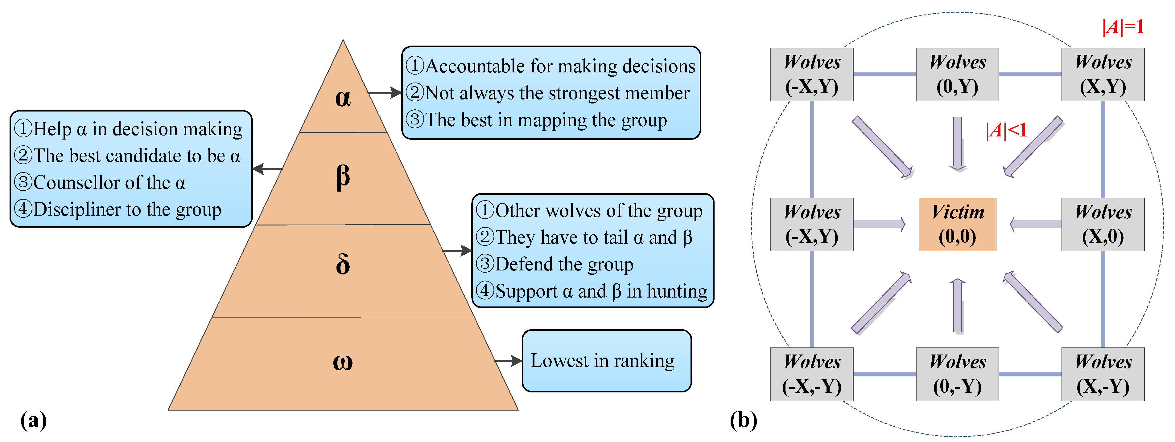
3.3. Grey Wolf Optimizer (GWO)

The grey wolf optimizer (GWO) algorithm is a meta-heuristic algorithm, which was first proposed by Mirjalili, et al. [134]. The purpose is to simulate the life habits of grey wolves in nature under the premise of the optimization algorithm [53,135]. Grey wolf is a kind of simulation of leadership and living according to the social dominance hierarchy [136]. In the social hierarchy of grey wolves, there are four roles: decision maker (α), facilitator (β), executor (δ) and nanny (ω) (Figure 4). Among them, the decision maker (α) as the leader represents the highest social status. All other characters are controlled by alpha wolves [137]. The facilitator (β) helps alpha wolves make decisions and establish herd discipline [134]. When alpha wolves retire or die, beta wolves are also the most suitable substitute for alpha [138]. The executor (δ) obeys alpha wolves and beta wolves, and exists as a hunter, scout, and watcher. The nanny (ω) exists to maintain internal harmony. It acts as a guilty sheep or nanny, and is at the bottom of the grey wolves pack society. However, without the existence of omega wolves, it is difficult to maintain the stability of the above three roles, and internal battles may break out at any time. The main social behavior of grey wolves is to obtain hunting prey corresponding to the social hierarchy [138,139,140]. Then it can be considered to collect randomly preferred solutions through the GWO meta-heuristic algorithm with optimization process [141]. Specifically, α, β, δ, and ω are respectively regarded as the optimal solution, the second preferred, the third preferred and the remaining solutions [142]. The GWO model mainly includes three steps: (1) approaching the target and surrounding behavior; (2) hunting behavior; (3) attacking the target and exploiting behavior [138,143]. First, the grey wolves pack encircles, and the digital model can be expressed as [134]:

$$\begin{array}{l}\overrightarrow{D}=\left|\overrightarrow{C}\cdot {\overrightarrow{X}}_{victim}(t)-{\overrightarrow{X}}_{wolf}(t)\right|\\ {\overrightarrow{X}}_{wolf}(t+1)={\overrightarrow{X}}_{victim}(t)-\overrightarrow{A}\cdot \overrightarrow{D}\end{array}$$

(8)

where, $\overrightarrow{A}$, $\overrightarrow{C}$ and $\overrightarrow{D}$ denote coefficient vectors, ${\overrightarrow{X}}_{wolf}(t)$ and ${\overrightarrow{X}}_{victim}(t)$ represent the current positions of the grey wolves and victim respectively (Figure 4), and t represents the current iteration. Next, it performs hunting behavior. The position of ω can be changed by the optimal solution of α, β and δ wolves’ position [144]. The new position of the grey wolves for α, β and δ can be calculated by the following formula:

$$\begin{array}{l}{\overrightarrow{D}}_{\alpha }=\left|{\overrightarrow{C}}_1\cdot {\overrightarrow{X}}_{\alpha }(t)-{\overrightarrow{X}}_{wolf}(t)\right|\\ {\overrightarrow{D}}_{\beta }=\left|{\overrightarrow{C}}_2\cdot {\overrightarrow{X}}_{\beta }(t)-{\overrightarrow{X}}_{wolf}(t)\right|\\ {\overrightarrow{D}}_{\delta }=\left|{\overrightarrow{C}}_3\cdot {\overrightarrow{X}}_{\delta }(t)-{\overrightarrow{X}}_{wolf}(t)\right|\\ {\overrightarrow{D}}_1={\overrightarrow{X}}_{\alpha }-{\overrightarrow{A}}_1{\overrightarrow{D}}_{\alpha }\\ {\overrightarrow{D}}_2={\overrightarrow{X}}_{\beta }-{\overrightarrow{A}}_2{\overrightarrow{D}}_{\beta }\\ {\overrightarrow{D}}_3={\overrightarrow{X}}_{\delta }-{\overrightarrow{A}}_3{\overrightarrow{D}}_{\delta }\\ {\overrightarrow{X}}_{wolf}(t+1)=({\overrightarrow{X}}_1+{\overrightarrow{X}}_2+{\overrightarrow{X}}_3)/3\end{array}$$

(9)

Finally, the main goal is to determine the best location of victim. Wolf behavior is determined by the value of |A|. When |A| > 1 deviates from the victim and |A| < 1 converges to the victim. When the standard value of |A| = 1 is reached, the optimization of GWO will be realized [134].

3.4. Firefly Algorithm (FA)

The firefly algorithm (FA), as a modern meta-heuristic algorithm, was proposed by Yang [145] and inspired by the social behavior of tropical summer fireflies flashing in the sky [146]. Fireflies exchange information and seek behavior based on the bioluminescence of different flash patterns [147]. FA realizes the idealization of the luminous characteristics of fireflies. It follows three rules:

(1) All fireflies have no gender distinction, and any one firefly will attract all other fireflies; (2) the attracting ability of a firefly is positively related to its luminous intensity. The brighter fireflies will attract other fireflies that are not brighter. When there is no firefly brighter than a particular firefly in the space, it will move randomly; (3) the brightness of the firefly depends on the value of its objective function, which guides the search process.

The entire firefly population is randomly distributed in the two-dimensional search space. In this case, assume that the search space has one best global (BG) value and two best local (BL) values (so there are three best values in total). Throughout the initial search process, some fireflies moved toward the best global (BG) value, and some moved toward the best local (BL) value (Figure 5) [148].

For the maximization problem, the brightness of the firefly can be regarded as proportional to the value of the cost function (brightness = objective function) [148]. In order to obtain a more reasonable FA, it is necessary to pay special attention to the light intensity change and the attraction formula.

The light intensity change (I) of the firefly can get all possible solutions of the fitness function of I(s) and F(s), and the value of I(r) can be obtained according to the following formula [149,150]:

$$I=I_0{e}^{-vr}$$

(10)

where I₀ represents the light intensity of the light source, and a fixed light absorption coefficient v is used to estimate light absorption. By integrating the inverse square law and the influence of the Gaussian absorption approximation, the singularity at r = 0 in the expression I/r² is avoided. A parallel relationship with the above formula can be introduced to explain the attractive force (P):

$$P=P_0{e}^{-v{r}^2}$$

(11)

where P₀ is the attractive force when r = 0. To some extent, the light intensity I and the attractive force P are equal. The distance between any two firefly X_i and X_j is expressed according to the Euclidean distance of the basic firefly algorithm [149,150]:

$$rij=\Vert X_i-X_j\Vert =\sqrt{{\displaystyle {\sum }_{k=1}^n\left(X_{i,k}-X_{j,k}\right)}}$$

(12)

where n represents the dimensionality of the problem. The movement of the i-th firefly is attracted by another more attractive firefly j. Thus, the following equation is applied:

$$x_i=x_i+P_0{e}^{-v{r}_{ij}^2}\left(x_i-x_j\right)+\lambda {\sigma }_i$$

(13)

where ${\sigma }_i$ is a random number extracted from Gaussian distribution [149]. In the above formula, the parameter λ can be changed from 0 to 1 [151].

4. Results

4.1. Correlation Analysis and Selection of Conditioning Factors

In this study, the average merit (AM) of each conditioning factor was calculated by using the correlation attribute evaluation (CAE) and 10-fold cross-validation [152], and the results are shown in Figure 6. The results show that all the 16 factors can promote the occurrence of a landslide (AM > 0). The results show that elevation has the greatest effect on landslide occurrence (AM = 0.407), followed by NDVI (AM = 0.373), soil (AM = 0.356), land use (AM = 0.328), distance to rivers (AM = 0.316), distance to roads (AM = 0.314), distance to faults (AM = 0.183), lithology (AM = 0.184), slope (AM = 0.182), aspect (AM = 0.175), rainfall (AM = 0.103), plan curvature (AM = 0.047), profile curvature (AM = 0.031), SPI (AM = 0.03), STI (AM = 0.024) and TWI (AM = 0.007). Therefore, all the factors are adopted in this study.

The frequency ratio (FR) model is also used to measure the correlation between landslide and conditioning factors. It can be clearly seen from

Table 2. Correlation between landslides and conditioning factors using frequency ratio (FR) model.

Conditioning Factors	Classes	Percentage of Domain (a)	Percentage of Landslides (b)	FR (b/a)
Elevation (m)	547–700	0.7	0.6	0.90
	700–900	3.5	10.9	3.09
	900–1100	9.4	35.7	3.80
	1100–1300	14.9	24.0	1.61
	1300–1500	17.2	11.9	0.70
	1500–1700	16.6	7.8	0.47
	1700–1900	14.8	1.3	0.09
	1900–2100	10.6	2.7	0.26
	2100–2300	6.7	1.9	0.29
	2300–2500	4.0	3.2	0.80
	2500–2700	1.4	0.0	0.00
	2700–2911	0.2	0.0	0.00
Slope (°)	0–10	5.8	0.0	0.00
	10–20	19.6	11.8	0.60
	20–30	30.9	31.7	1.03
	30–40	28.1	35.3	1.26
	40–50	13.4	17.7	1.32
	50–60	2.2	3.6	1.62
	60–72.77	0.1	0.0	0.00
Aspect (°)	Flat (−1)	0.0	0.0	0.00
	North (0°–22.5°)	13.1	0.1	0.01
	Northeast (22.5°–67.5°)	14.3	0.8	0.06
	East (67.5°–112.5°)	13.8	15.6	1.13
	Southeast (112.5°–157.5°)	12.5	42.8	3.42
	South (157.5°–202.5°)	12.2	31.5	2.60
	Southwest (202.5°–247.5°)	12.0	7.0	0.59
	West (247.5°–292.5°)	11.6	2.0	0.17
	Northwest (292.5°–337.5°)	10.6	0.2	0.02
Plan curvature (m/100)	Concave	47.5	52.6	1.11
	Plan	4.3	3.7	0.87
	Convex	48.3	43.7	0.90
Profile curvature (m/100)	Concave	47.6	40.8	0.86
	Plan	3.0	1.9	0.63
	Convex	49.4	57.3	1.16
Distance to faults (m)	0–500	25.4	21.4	0.84
	500–1000	19.2	32.5	1.69
	1000–1500	14.9	12.0	0.81
	1500–2000	11.5	23.3	2.03
	>2000	29.0	10.8	0.37
Distance to rivers (m)	0–200	23.8	49.5	2.08
	200–400	19.5	27.2	1.39
	400–600	16.9	7.3	0.43
	600–800	14.6	6.7	0.46
	>800	25.2	9.4	0.37
Distance to roads (m)	0–200	6.8	26.8	3.95
	200–400	5.5	19.1	3.48
	400–600	5.1	6.8	1.34
	600–800	4.9	2.2	0.45
	>800	77.7	45.0	0.58
STI	0–10	42.8	30.1	0.70
	10–20	27.7	28.8	1.04
	20–30	10.9	13.4	1.23
	30–40	5.0	6.6	1.32
	>40	13.7	21.2	1.55
SPI	0–10	32.7	23.1	0.71
	10–20	16.9	14.6	0.86
	20–30	11.3	12.7	1.12
	30–40	6.8	7.1	1.05
	>40	32.3	42.6	1.32
TWI	<1.5	25.8	26.7	1.04
	1.5–2	36.8	33.8	0.92
	2–2.5	16.5	14.6	0.88
	2.5–3	9.3	14.6	1.57
	>3	11.6	10.3	0.89
NDVI	−0.12–0.16	6.6	1.4	0.21
	0.16–0.24	16.2	4.4	0.27
	0.24–0.31	23.9	8.8	0.37
	0.31–0.38	26.3	24.0	0.91
	0.38–0.53	26.9	61.5	2.29
Landuse	Farmland	11.0	26.3	2.40
	Forestland	43.3	13.0	0.30
	Grassland	45.5	60.6	1.33
	Water bodies	0.0	0.0	0.00
	Construction land	0.2	0.0	0.00
	Bare land	0.0	0.0	0.00
Rainfall (mm/yr)	<800	0.1	0.5	4.60
	800–850	0.2	0.0	0.00
	850–900	1.3	0.0	0.00
	900–950	4.2	3.1	0.75
	950–1000	35.0	22.1	0.63
	1000–1050	48.6	63.5	1.31
	1050–1100	7.4	7.7	1.04
	1100–1150	2.4	3.0	1.24
	1150–1200	0.8	0.2	0.24
	>1200	0.2	0.0	0.00
Soil	Type 1 (Yellow-brown soil)	23.4	28.7	1.23
	Type 2 (Dark-yellow-brown soil)	13.9	21.1	1.52
	Type 3 (Yellow-browning soil)	0.0	0.0	0.00
	Type 4 (Albic yellow cinnamon soil)	0.5	3.7	7.79
	Type 5 (Brown soil)	55.0	21.7	0.39
	Type 6 (Alluvial soil)	2.9	19.4	6.81
	Type 7 (Calcareous soil)	1.5	0.4	0.24
	Type 8 (Skeletal soil)	2.3	5.0	2.22
	Type 9 (Mountain scrubby-meadow soil)	0.6	0.0	0.00
Lithology	Group 1	2.5	0.2	0.07
	Group 2	6.9	5.7	0.84
	Group 3	1.2	0.0	0.00
	Group 4	0.9	1.5	1.62
	Group 5	1.8	1.1	0.60
	Group 6	24.7	36.0	1.46
	Group 7	44.6	40.2	0.90
	Group 8	7.8	7.4	0.95
	Group 9	7.9	7.3	0.92
	Group 10	1.8	0.6	0.35

that the area proportion statistics and landslide point proportion statistics of the 16 landslide conditioning factors in this paper are carried out in GIS software, and the frequency ratio (FR) value of each category is calculated. These weight values of FR represent the ratio of landslide occurrence rate to area ratio of conditioning factors [153,154]. The highest proportion of landslide points (35.73%) was found in the range of 900–1100 m, and the FR value was the largest (3.80) (Category 3). For the slope, the FR value (1.62) in the range of 50–60° is the largest (Category 6), while there is no landslide in the area greater than 60°. In the study area, the FR value is proportional to the slope angle. It can be understood that the shear pressure inside the soil generally increases with the increase of slope angle [154,155]. As for the relationship between slope aspect and landslide, the FR values in the Southeast (3.42) and South (2.60) ranges are larger (Category 5 and 6), indicating that these categories have positive spatial correlation with the occurrence of landslides [156]. In the range of the concave surface of the plan curvature (1.11, Category 1), the range of the convex surface of the profile curvature (1.16, Category 3), the distance to faults is in the range of 1500–2000 m (2.03, Category 4), the STI is in the range of >40 (1.55, Category 5), the SPI in the range of >40 (1.32, Category 5), the TWI in the range of 2.5–3 (1.57, Category 4), the NDVI in the range of 0.38–0.53 (2.29, Category 5), and the fourth group (group 4: metamorphic rhyolite, quartz porphyry, volcanic clastic rocks, phyllite, metamorphic sandstone) in the lithology (1.63) has the largest FR value and the highest probability of landslide occurrence. For the two conditioning factors of distance to rivers and distance to rivers, the smaller the distance, the greater the possibility of landslides. Because road construction always produces countless slopes, disturbing the stability of the slope results in a large number of landslides [157,158]. The river network sculpts and shapes the landform to a large extent. The supporting force of the river on the slope and the pore water pressure of the alternate slope are controlled. Therefore, in many cases in the previous studies, the distance from the river is a key adjustment factor [157,158]. In terms of land use, the FR value in farmland is the largest (2.40). This is closely related to land irrigation, human engineering activities and rainfall [159]. For rainfall, the largest FR value (4.64) appears in the range of <800 mm/yr. Regarding the relationship between soil and landslide, the higher FR values in the range of Type 4 (7.84) and Type 6 (6.82) indicate that landslides are most likely to occur in these categories.

4.2. Application of Hybrid Models

In this study, with training and testing as the basic principles, a single model of the SVR model and two hybrid models of the SVR-FA model and the SVR-GWO model were developed using the Matlab software. At this point, the prepared training dataset (70%) and testing dataset (30%) that have been preprocessed by the FR model come into play. These three models (SVR, SVR-GWO, and SVR-FA) firstly use training data samples to explore the relationship between landslide conditioning factors and landslides and non-landslides in the study area. Then, the testing dataset is used to verify the accuracy of the model built. Accuracy analysis is performed on the training data samples and testing data samples using the three models, and the results are shown in Figure 7, Figure 8 and Figure 9. The target and output value of the training data samples and the testing data samples are counted, and the mean standard error (MSE) and standard deviation (StD) are used to determine the accuracy of the two data samples. In the training data samples, the MSE values of the SVR, SVR-GWO and SVR-FA models are 0.042, 0.018 and 0.022, respectively; the StD values of frequency error are 0.205, 0.134 and 0.147, respectively. According to the size of MSE and StD, two hybrid models, SVR-GWO and SVR-FA, are selected as good models. A model that can obtain higher-precision results by verifying testing data samples can be considered as a more optimized model. Therefore, the statistical values of the testing data samples are shown in Figure 7, Figure 8 and Figure 9d–f. The MSE and StD values of the SVR model are 0.040 and 0.198, respectively, the MSE and StD values of the SVR-GWO model are 0.021 and 0.144, and the MSE and StD values of the SVR-FA model are 0.032 and 0.180, respectively. The results show that the SVR-GWO model is the best algorithm among the three models, and the single model SVR is the worst. This is because, in the accuracy analysis, they are the best and worst in the evaluation and prediction of training data samples and testing data samples, respectively.

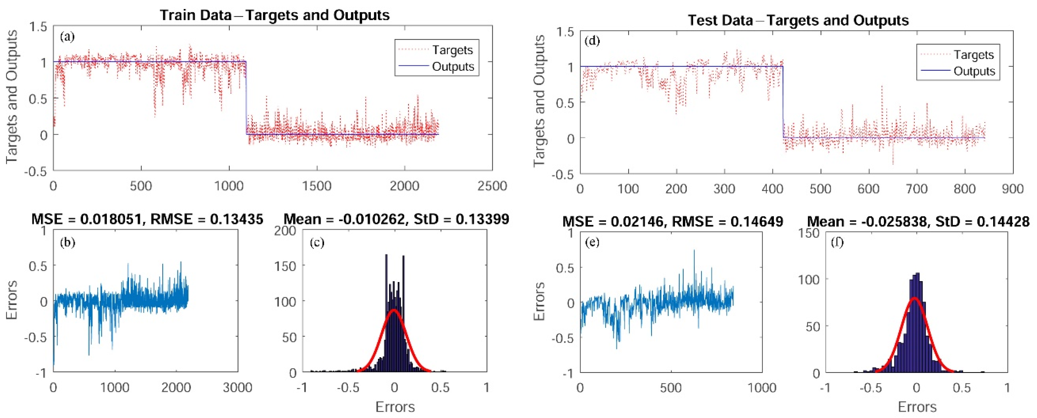
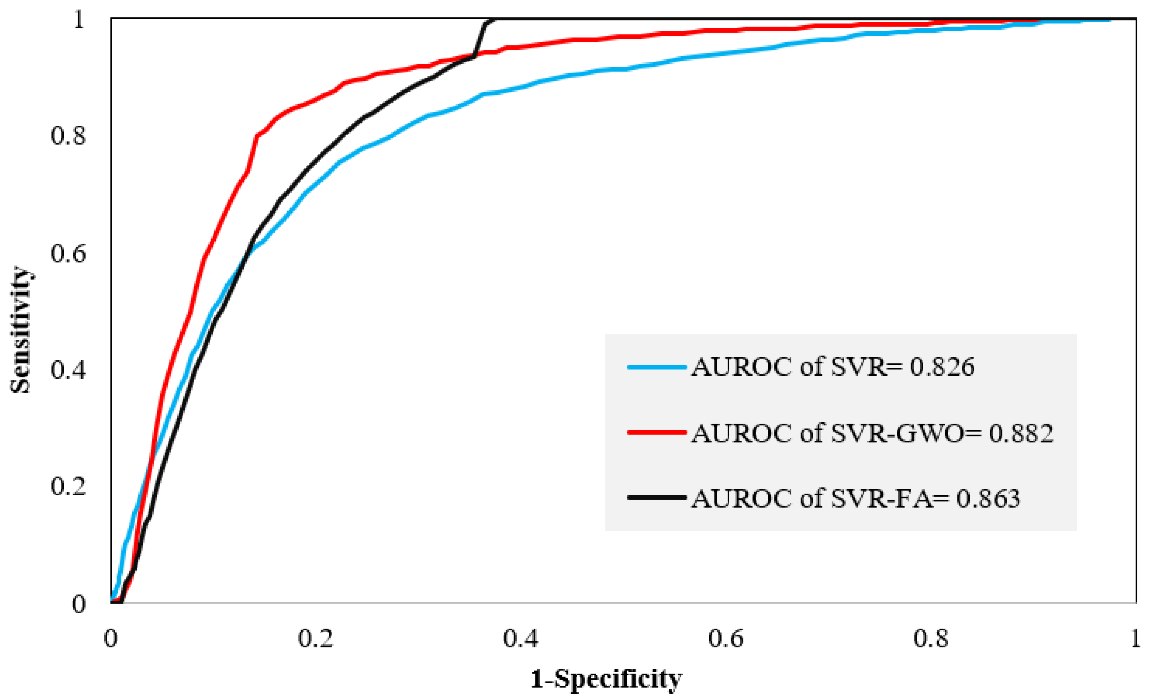
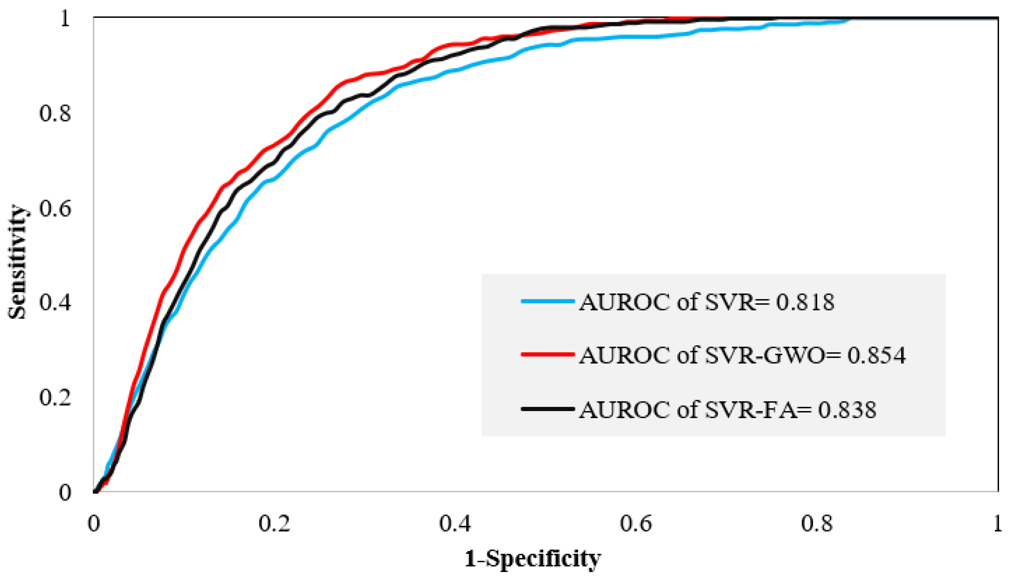
4.3. Validation and Comparison of Models

The validation of landslide susceptibility model is an important part of landslide susceptibility mapping [83]. The receiver operating characteristic (ROC) curve and the area under the receiver operating characteristic curve (AUROC) are used to evaluate the performance of the landslide susceptibility model. In the AUROC figure, the quality of classifier for probabilistic or deterministic landslide susceptibility model can be effectively represented [160]. The training and test datasets in the AUROC curve can be used to evaluate the goodness of fit (learning ability) and prediction ability (generalization) of the selected model, respectively [161]. The more area under the receiver operating characteristic curve (AUROC), the higher the performance of the model. The sensitivity of the model is expressed by the percentage of the number of landslide grids correctly predicted by the model, and the specificity is expressed by the percentage of the predicted grid number of landslides in the whole study area. The AUROC value represents the performance of the model. The AUROC value of the suitable model is distributed between 0.5–1. The closer to 1, the more perfect the model is. Figure 10 and Figure 11 show the AUROC curves of the selected landslide susceptibility model from the training dataset and the validation dataset, respectively. All models performed well in landslide susceptibility assessment (AUC > 0.810). The AUROC values of the model in the training dataset and the validation dataset are in the same order. In the training dataset, the SVR-GWO model (AUROC = 0.882) has the best, followed by the SVR-RA model (AUROC = 0.863) and the SVR model (AUROC = 0.826). In the validation dataset, the performance of the SVR-GWO model (AUROC = 0.854) is better than the SVR-RA model (AUROC = 0.838) and the SVR model (AUROC = 0.818). Therefore, the SVR-GWO model can be considered as the best model.

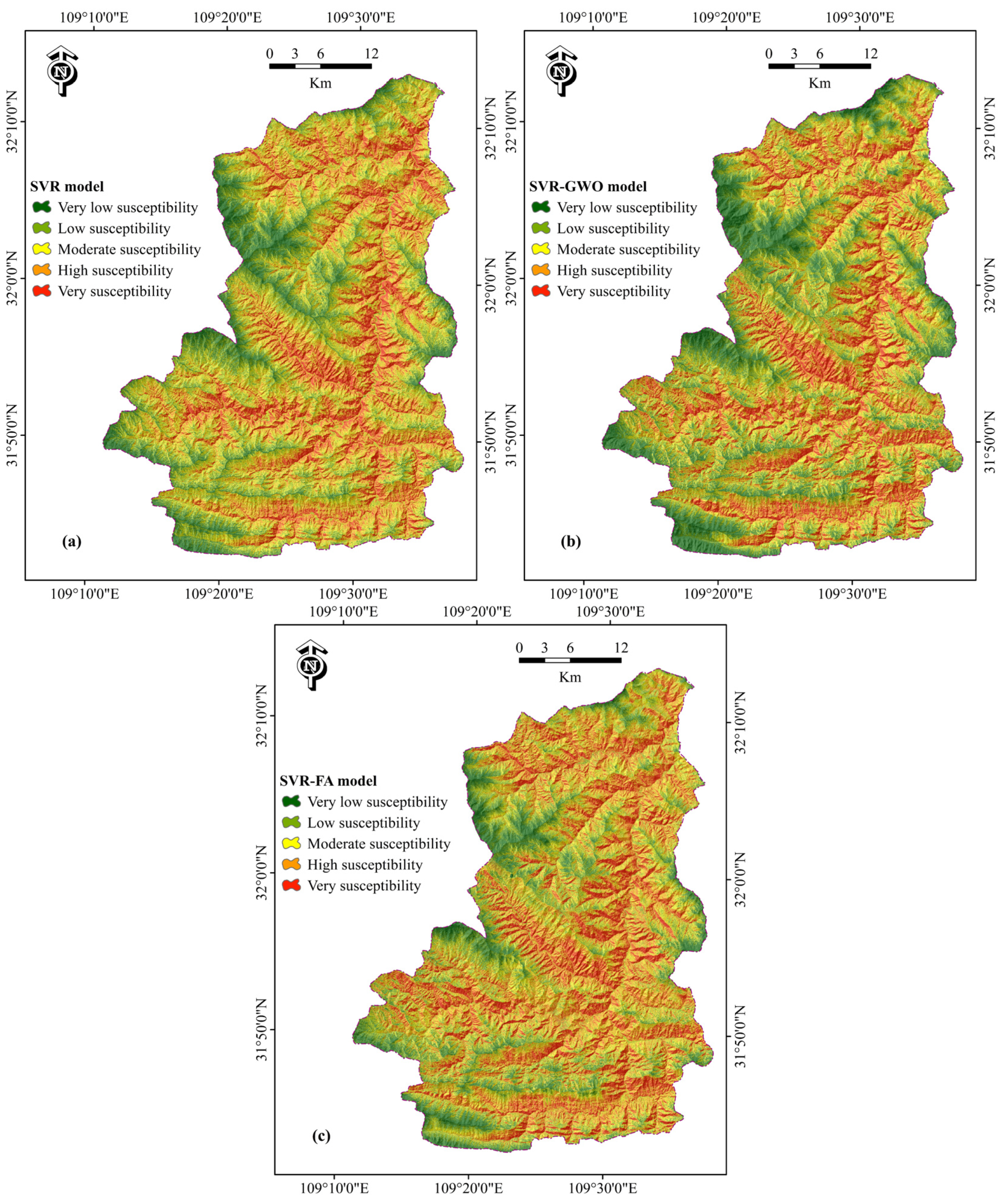
4.4. Generation of Landslide Susceptibility Maps

In this paper, the landslide susceptibility index (LSI) is calculated for the three selected models. LSI can be regarded as the probability value of 0 to 1. The higher the LSI, the greater the possibility of landslide. After the corresponding LSI values are attached to each pixel in the study area, the final landslide susceptibility map is generated in GIS. The three landslide susceptibility maps generated by the SVR model, SVR-GWO model and SVR-FA model are shown in Figure 12.

The landslide susceptibility map of the study area is divided by the Jenks natural breaks method, including very low susceptibility area, low susceptibility area, moderate susceptibility area, high susceptibility area and very high susceptibility area. In three different models, the area proportion of each category was calculated (Figure 13). For the SVR model, the highest proportion was the moderate susceptibility area (27.66%), followed by the high susceptibility area (26.48%), the low susceptibility area (21.16%), the very high susceptibility area (14.42%), and the very low susceptibility area (10.28%). According to the results of the SVR-GWO model, the areas with very low susceptibility (15.89%), low susceptibility (22.97%), moderate susceptibility (23.69%), high susceptibility (22.10%) and very high susceptibility (15.35%) were classified and distributed. In the SVR-FA model, the proportion of very low, low, moderate, high and very high susceptibility areas were 10.39%, 19.12%, 25.10%, 26.68% and 18.71%, respectively.

In addition, although AUROC can directly reflect the proportion of correct classification, the sample size of each category is often unbalanced. Therefore, three values, including Kappa index, kappa location and kappa histogram, were calculated for all regions and five subregions by kappa statistics using the Map Comparison Kit (MCK) software [162,163]. Kappa location and kappa histogram are extensions of Kappa index [163]. The values of kappa statistics vary from 0 to 1. A value of 1 indicates that the two classes are identical (exactly the same), and a value of 0 indicates that the two classes are inconsistent [164]. It can be considered that the kappa value of 0.8–1.0 indicates that the similarity is almost perfect, 0.6–0.8 indicates high similarity, 0.4–0.6 indicates medium similarity, 0.2–0.4 indicates poor similarity, and 0–0.2 indicates extremely poor similarity [164,165].

The comparison results of kappa statistics data of three landslide susceptibility maps are shown in

Table 3. Kappa statistics of landslide susceptibility maps.

Landslide Susceptibility Map	Very Low	Low	Moderate	High	Very High	All
SVR vs. SVR-GWO
Kappa index	1.000	0.680	0.477	0.426	0.747	0.586
Kappa location	1.000	0.878	0.491	0.476	0.780	0.640
Kappa histogram	1.000	0.775	0.972	0.896	0.957	0.916
SVR vs. SVR-FA
Kappa index	1.000	0.608	0.418	0.326	0.659	0.503
Kappa location	1.000	0.612	0.446	0.349	0.725	0.539
Kappa histogram	1.000	0.937	0.937	0.934	0.909	0.934
SVR-GWO vs. SVR-FA
Kappa index	1.000	0.658	0.413	0.339	0.711	0.536
Kappa location	1.000	0.843	0.454	0.352	0.821	0.604
Kappa histogram	1.000	0.780	0.909	0.962	0.856	0.888

. The results show that the three susceptibility maps have exactly the same similarity in the very low susceptibility area, and the kappa value is 1.

In the low susceptibility area, the index similarity of the three susceptibility maps is higher, and the similarity of location and quantity also have higher and almost perfect results. In the moderate susceptibility area, the index similarity of the three susceptibility maps is moderate, the position similarity is consistent with the index similarity, and the quantitative similarity among them is almost perfect. In the high susceptibility area, the kappa index of the SVR and SVR-GWO models is the largest (0.426), followed by the kappa index of the SVR-GWO and SVR-FA models (0.339), and the kappa index of the SVR and SVR-FA models (0.326), indicating that the similarity of the pairwise comparison group is medium or poor. At the same time, the positional similarity is consistent with the index similarity, and the quantitative similarity is still almost perfect. In the very high susceptibility area, the similarity of the three susceptibility maps is high, and the location similarity also has high and almost perfect results, and the quantitative similarity is almost perfect. On the whole of the study area, the kappa index of the three susceptibility maps is between 0.503 and 0.586, indicating that the similarities of the susceptibility maps are medium. The location similarity also has medium and high results, indicating that the spatial distribution of the three types of landslide susceptibility maps is not closely related. At the same time, the quantitative similarity is almost perfect, indicating that the number of landslides in each landslide susceptibility map has perfect quantitative correlation.

5. Discussion

Zhenping County is located in the hinterland of Daba Mountain, with a complex geological environment, high mountains, deep gullies and steep slopes. The landslide disasters in the study area are widely distributed, numerous and harmful. Landslide susceptibility modeling and optimization has a great impact on the regional evaluation of landslide disasters. The modeling methods are various and involve a wide range of contents, which is of great significance. Landslide susceptibility prediction is regarded as the first means of land use planning, which is also the first important step of landslide hazard and risk assessment [166]. Therefore, it is necessary to choose an effective landslide susceptibility model for modeling.

In this study, 140 landslides and 16 landslide conditioning factors were selected for data preparation. The FR algorithm was used to analyze the spatial correlation between landslides and the condition factors. In terms of elevation, the FR value decreases with the increase of elevation. This is mainly due to the impact of human activities in low-altitude areas and high-altitude anti-weathering rocks [117,167]. On the other hand, another important reason is the impact of heavy rain on low altitude area [160]. The slope is directly proportional to the FR value, which is also based on local conditions. At the same time, it can be clearly seen that the FR values in the southeast and south directions are the largest, mainly due to the influence of sunshine and rainfall. After more dry and wet cycles, the soil strength in the southeast and south directions is weakened. The plan and profile curvatures show abnormal results. The concave plan curvature and convex profile curvature can compensate slope by the concentrating water and the corresponding shear stress [160]. The linear characteristics of distance to faults, distance to rivers and distance to roads are inversely proportional to the landslide susceptibility (FR value). As the SPI increases, the FR value increases. NDVI is directly proportional to landslide susceptibility, in part because strong wind will increase the weight of vegetation, thus forcing additional downward load on the slope [160,168]. There are more irrigation and artificial excavation effects in farmland and grassland areas, which affect the stability of landslide and have high landslide susceptibility. As for lithology, the dominant categories include the fourth group (Proterozoic: metamorphic rhyolite, quartz porphyry, volcanic clastic rocks, phyllite, metamorphic sandstone) and the sixth group (Silurian: slate, argillaceous limestone, banded slate, carbonaceous slate, silt sandstone, sandstone). There is groundwater flow in saturated sandstones that are relatively easy to crack and rocks with cracks, which cause additional loads on the rocks, resulting in a faster penetration process, which leads to landslides.

The standard guidelines for the selection of factors are still a topic of debate [169]. The contribution of factors depends on the distribution characteristics of landslides, the geo-environmental characteristics of the study area, and the evaluation method used. In this study, the selection of landslide conditioning factors using the correlation attribute evaluation (CAE) and 10-fold cross-validation indicated that the 16 landslide conditioning factors have positive contributions to landslide models. The elevation (0.407), NDVI (0.373), and soil (0.356) have the highest importance, while TWI (0.007), STI (0.024) and SPI (0.03) show lower predictive ability. Therefore, further studies are necessary to explore landslide conditioning factor selection methods.

A single SVR model and two hybrid models of SVR-GWO and SVR-FA were established for landslide susceptibility assessment. Statistics and analysis of the target value and output value of the training data samples and the testing data samples are carried out on the training dataset and the testing dataset of the three models. It can be seen intuitively from the images of each model that the SVR-GWO model is more regular, including the curve of target value and output value, the curve of error distribution, and the histogram of error quantity. It can be clearly seen from the accuracy analysis parameters that the errors of the hybrid models are smaller than that of the single model, and the SVR-GWO model is the best algorithm.

When using the AUROC curve to evaluate the performance of the model, it was found that the three landslide susceptibility models (SVR, SVR-GWO and SVR-FA) expressed their good quality in the form of probability. At the same time, the performance of the model is stable and reliable in both the training dataset and the testing dataset. After comparison, it is found that the two hybrid models improve the performance of the single model, and it can be considered that the three models perform well. Among them, the SVR-GWO model (0.854) is the best model, followed by the SVR-FA (AUROC = 0.838) and SVR models (AUROC = 0.818).

In this study, the three hybrid models used LSI values to obtain a robust landslide susceptibility assessment and mapping. The three landslide susceptibility maps are composed of SVR, SVR-GWO and SVR-FA models preprocessed by FR algorithm. The three landslide susceptibility maps and the histogram with five susceptibility areas show intuitively and visually the application of the model to the landslide susceptibility of the Zhenping County study area. The hybrid model improves the performance and partition accuracy of the SVR single model. The partition results of the three models all have a reasonable distribution, and the SVR-GWO model obtains the best partition results. For the SVR-FA model and the SVR model, the area in the high-susceptibility region is smaller than that of the SVR-GWO model. This reduces the time and cost for effective mitigation plans in those target areas of disaster prevention and land use planning.

In addition, the performance of the three models is judged from the kappa data. The most obvious is the extremely high similarity in numbers, indicating that the five subregions in each model divide the landslides reasonably and reliably. The biggest difference between the models is the SVR and SVR-FA models, followed by the SVR-GWO and SVR-FA models, indicating that the tendency of over-adaptation between the models is small. With reference to the previous AUROC value, it also shows that the integration of the model positively affects the performance of the model. These are labels indicating that the three hybrid models have good performance and reliable results.

In general, in order to obtain better landslide susceptibility modeling results, it is a wise approach to adopt a hybrid algorithm. The two hybrid algorithms (SVR-GWO is better than SVR-FA) in this paper are better than its own single model (SVR) when applied to the Zhenping County study area. These three models can be applied to regional-scale landslide spatial modeling in other regions. At the same time, the three landslide susceptibility maps in this article can provide government personnel, land use planners and engineers with a basis for land use planning.

6. Conclusions

Landslide is one of the disasters with clear social attributes that cannot be ignored. In this study, the performance of the hybrids of support vector regression (SVR), grey wolf optimizer (GWO) and firefly algorithm (FA) algorithm in landslide susceptibility assessment of Zhenping County is compared, which is the main novelty of the paper. The frequency ratio (FR) algorithm is used to evaluate the relationship between landslide and conditioning factors. In the process of factor selection analysis, elevation, NDVI, soil, land use, distance to rivers, and distance to roads are the most important conditioning factors. On this basis, the hybrid models are used for landslide spatial prediction of the study area. The results show that the SVR-GWO model (AUROC = 0.854) has better prediction accuracy than the SVR-FA (AUROC = 0.838) and SVR model (AUROC = 0.818). In addition, three landslide susceptibility maps are drawn and analyzed, and the advantages and disadvantages of the landslide susceptibility model are obtained from the proportion of five susceptibility areas and kappa data. The results of this study show that the three hybrid models processed based on GIS can be successfully applied to landslide susceptibility mapping in Zhenping County. It is a useful tool for the sustainable development of land management with low cost of capital and time. The SVR-GWO model could be used to accurately assess the spatial susceptibility of landslides in Zhenping County, Shaanxi Province, China. It provides early theoretical support for local government decision-makers and engineering designers. At the same time, other areas under similar environmental conditions can also be evaluated by the same method.

References

1. Pham, B.T.; Tien Bui, D.; Prakash, I. Bagging based Support Vector Machines for spatial prediction of landslides. Environ. Earth Sci. 2018, 77, 146. [Google Scholar] [CrossRef]
2. Varnes, D.J. Landslide Hazard Zonation: A Review of Principles and Practice; TRID: Jacksonville, FL, USA, 1984. [Google Scholar]
3. Zhou, C.; Yin, K.; Cao, Y.; Ahmed, B.; Li, Y.; Catani, F.; Pourghasemi, H.R. Landslide susceptibility modeling applying machine learning methods: A case study from Longju in the Three Gorges Reservoir area, China. Comput. Geosci. 2018, 112, 23–37. [Google Scholar] [CrossRef] [Green Version]
4. Mahalingam, R.; Olsen, M.J. Evaluation of the influence of source and spatial resolution of DEMs on derivative products used in landslide mapping. Geomat. Nat. Hazards Risk 2015, 7, 1835–1855. [Google Scholar] [CrossRef]
5. Pham, B.T.; Tien Bui, D.; Pourghasemi, H.R.; Indra, P.; Dholakia, M.B. Landslide susceptibility assesssment in the Uttarakhand area (India) using GIS: A comparison study of prediction capability of naïve bayes, multilayer perceptron neural networks, and functional trees methods. Theor. Appl. Climatol. 2017, 128, 255–273. [Google Scholar] [CrossRef]
6. Pham, B.T.; Nguyen, V.-T.; Ngo, V.-L.; Trinh, P.T.; Ngo, H.T.T.; Tien Bui, D. A novel hybrid model of rotation forest based functional trees for landslide susceptibility mapping: A case study at kon tum province, vietnam. In Advances and Applications in Geospatial Technology and Earth Resources; Tien Bui, D., Ngoc Do, A., Bui, H.-B., Hoang, N.-D., Eds.; Springer International Publishing: Berlin/Heidelberg, Germany, 2017; pp. 186–201. [Google Scholar]
7. Ercanoglu, M.; Gokceoglu, C.; Van Asch, T.W.J. Landslide Susceptibility Zoning North of Yenice (NW Turkey) by Multivariate Statistical Techniques. Nat. Hazards 2004, 32, 1–23. [Google Scholar] [CrossRef]
8. Rasyid, A.; Bhandary, N.; Yatabe, R. Performance of frequency ratio and logistic regression model in creating GIS based landslides susceptibility map at Lompobattang Mountain, Indonesia. Geoenviron. Disasters 2016, 3, 19. [Google Scholar] [CrossRef] [Green Version]
9. Bălteanu, D.; Micu, M.; Jurchescu, M.; Malet, J.-P.; Sima, M.; Kucsicsa, G.; Dumitrică, C.; Petrea, D.; Mărgărint, M.C.; Bilaşco, Ş.; et al. National-scale landslide susceptibility map of Romania in a European methodological framework. Geomorphology 2020, 371, 107432. [Google Scholar] [CrossRef]
10. Aditian, A.; Kubota, T.; Shinohara, Y. Comparison of GIS-based landslide susceptibility models using frequency ratio, logistic regression, and artificial neural network in a tertiary region of Ambon, Indonesia. Geomorphology 2018, 318, 101–111. [Google Scholar] [CrossRef]
11. Clerici, A.; Perego, S.; Tellini, C.; Vescovi, P. A procedure for landslide susceptibility zonation by the conditional analysis method. Geomorphology 2002, 48, 349–364. [Google Scholar] [CrossRef]
12. Süzen, M.L.; Doyuran, V. Data driven bivariate landslide susceptibility assessment using geographical information systems: A method and application to Asarsuyu catchment, Turkey. Eng. Geol. 2004, 71, 303–321. [Google Scholar] [CrossRef]
13. Al-Najjar, H.A.H.; Pradhan, B.; Sarkar, R.; Beydoun, G.; Alamri, A. A New Integrated Approach for Landslide Data Balancing and Spatial Prediction Based on Generative Adversarial Networks (GAN). Remote Sens. 2021, 13, 4011. [Google Scholar] [CrossRef]
14. Pradhan, B. A comparative study on the predictive ability of the decision tree, support vector machine and neuro-fuzzy models in landslide susceptibility mapping using GIS. Comput. Geosci. 2013, 51, 350–365. [Google Scholar] [CrossRef]
15. Westen, C.J.V.; Rengers, N.; Terlien, M.T.J.; Soeters, R. Prediction of the occurrence of slope instability phenomenal through GIS-based hazard zonation. Geol. Rundsch. 1997, 86, 404–414. [Google Scholar] [CrossRef]
16. Sestraș, P.; Bilașco, Ș.; Roșca, S.; Naș, S.; Bondrea, M.V.; Gâlgău, R.; Vereș, I.; Sălăgean, T.; Spalević, V.; Cîmpeanu, S.M. Landslides Susceptibility Assessment Based on GIS Statistical Bivariate Analysis in the Hills Surrounding a Metropolitan Area. Sustainability 2019, 11, 1362. [Google Scholar] [CrossRef] [Green Version]
17. Razandi, Y.; Pourghasemi, H.R.; Neisani, N.S.; Rahmati, O. Application of analytical hierarchy process, frequency ratio, and certainty factor models for groundwater potential mapping using GIS. Earth Sci. Inform. 2015, 8, 867–883. [Google Scholar] [CrossRef]
18. Wang, X.L.; Zhang, L.Q.; Ding, J.X.; Meng, Q.F.; Iqbal, J.; Li, L.H.; Yang, Z.F. Comparison of rockfall susceptibility assessment at local and regional scale: A case study in the north of Beijing (China). Environ. Earth Sci. 2014, 72, 4639–4652. [Google Scholar] [CrossRef]
19. Choi, J.; Oh, H.J.; Lee, H.J.; Lee, C.; Lee, S. Combining landslide susceptibility maps obtained from frequency ratio, logistic regression, and artificial neural network models using ASTER images and GIS. Eng. Geol. 2012, 124, 12–23. [Google Scholar] [CrossRef]
20. Yilmaz, I. Landslide susceptibility mapping using frequency ratio, logistic regression, artificial neural networks and their comparison: A case study from Kat landslides (Tokat—Turkey). Comput. Geosci. 2009, 35, 1125–1138. [Google Scholar] [CrossRef]
21. Pradhan, B. Landslide susceptibility mapping of a catchment area using frequency ratio, fuzzy logic and multivariate logistic regression approaches. J. Indian Soc. Remote Sens. 2010, 38, 301–320. [Google Scholar] [CrossRef]
22. Dou, J.; Oguchi, T.; Hayakawa, Y.S.; Uchiyama, S.; Saito, H.; Paudel, U. Gis-based landslide susceptibility mapping using a certainty factor model and its validation in the chuetsu area, central japan. In Landslide Science for a Safer Geoenvironment; Sassa, K., Canuti, P., Yin, Y., Eds.; Springer International Publishing: Berlin/Heidelberg, Germany, 2014; pp. 419–424. [Google Scholar]
23. Wang, Q.; Li, W.; Chen, W.; Bai, H. GIS-based assessment of landslide susceptibility using certainty factor and index of entropy models for the Qianyang County of Baoji city, China. J. Earth Syst. Sci. 2015, 124, 1399–1415. [Google Scholar] [CrossRef]
24. Sujatha, E.R.; Rajamanickam, G.V.; Kumaravel, P. Landslide susceptibility analysis using Probabilistic Certainty Factor Approach: A case study on Tevankarai stream watershed, India. J. Earth Syst. Sci. 2012, 121, 1337–1350. [Google Scholar] [CrossRef] [Green Version]
25. Devkota, K.C.; Regmi, A.D.; Pourghasemi, H.R.; Yoshida, K.; Pradhan, B.; Ryu, I.C.; Dhital, M.R.; Althuwaynee, O.F. Landslide susceptibility mapping using certainty factor, index of entropy and logistic regression models in GIS and their comparison at Mugling–Narayanghat road section in Nepal Himalaya. Nat. Hazards 2013, 65, 135–165. [Google Scholar] [CrossRef]
26. Pourghasemi, H.R.; Pradhan, B. Application of weights-of-evidence and certainty factor models and their comparison in landslide susceptibility mapping at Haraz watershed, Iran. Arab. J. Geosci. 2013, 6, 2351–2365. [Google Scholar] [CrossRef]
27. Jebur, M.N.; Pradhan, B.; Tehrany, M.S. Optimization of landslide conditioning factors using very high-resolution airborne laser scanning (LiDAR) data at catchment scale. Remote Sens. Environ. 2014, 152, 150–165. [Google Scholar] [CrossRef]
28. Kayastha, P.; Dhital, M.R.; De Smedt, F. Landslide susceptibility mapping using the weight of evidence method in the Tinau watershed, Nepal. Nat. Hazards 2012, 63, 479–498. [Google Scholar] [CrossRef]
29. Ozdemir, A.; Altural, T. A comparative study of frequency ratio, weights of evidence and logistic regression methods for landslide susceptibility mapping: Sultan Mountains, SW Turkey. J. Asian Earth Sci. 2013, 64, 180–197. [Google Scholar] [CrossRef]
30. Lee, S.; Choi, J. Landslide susceptibility mapping using GIS and the weight-of-evidence model. Int. J. Geogr. Inf. Sci. 2004, 18, 789–814. [Google Scholar] [CrossRef]
31. Regmi, N.R.; Giardino, J.R.; Vitek, J.D. Modeling susceptibility to landslides using the weight of evidence approach: Western Colorado, USA. Geomorphology 2010, 115, 172–187. [Google Scholar] [CrossRef]
32. Pradhan, B. Use of GIS-based fuzzy logic relations and its cross application to produce landslide susceptibility maps in three test areas in Malaysia. Environ. Earth Sci. 2011, 63, 329–349. [Google Scholar] [CrossRef]
33. Aksoy, B.; Ercanoglu, M. Landslide identification and classification by object-based image analysis and fuzzy logic: An example from the Azdavay region (Kastamonu, Turkey). Comput. Geosci. 2012, 38, 87–98. [Google Scholar] [CrossRef]
34. Saboya, F.; Alves, M.D.G.; Pinto, W.D. Assessment of failure susceptibility of soil slopes using fuzzy logic. Eng. Geol. 2006, 86, 211–224. [Google Scholar] [CrossRef]
35. Pourghasemi, H.R.; Pradhan, B.; Gokceoglu, C. Application of fuzzy logic and analytical hierarchy process (AHP) to landslide susceptibility mapping at Haraz watershed, Iran. Nat. Hazards 2012, 63, 965–996. [Google Scholar] [CrossRef]
36. Zhu, A.X.; Wang, R.; Qiao, J.; Qin, C.-Z.; Chen, Y.; Liu, J.; Du, F.; Lin, Y.; Zhu, T. An expert knowledge-based approach to landslide susceptibility mapping using GIS and fuzzy logic. Geomorphology 2014, 214, 128–138. [Google Scholar] [CrossRef]
37. Ahmed, B. Landslide susceptibility mapping using multi-criteria evaluation techniques in Chittagong Metropolitan Area, Bangladesh. Landslides 2015, 12, 1077–1095. [Google Scholar] [CrossRef] [Green Version]
38. Komac, M. A landslide susceptibility model using the analytical hierarchy process method and multivariate statistics in perialpine Slovenia. Geomorphology 2006, 74, 17–28. [Google Scholar] [CrossRef]
39. Rozos, D.; Bathrellos, G.D.; Skillodimou, H.D. Comparison of the implementation of rock engineering system and analytic hierarchy process methods, upon landslide susceptibility mapping, using GIS: A case study from the Eastern Achaia County of Peloponnesus, Greece. Environ. Earth Sci. 2011, 63, 49–63. [Google Scholar] [CrossRef]
40. Yalcin, A. GIS-based landslide susceptibility mapping using analytical hierarchy process and bivariate statistics in Ardesen (Turkey): Comparisons of results and confirmations. Catena 2008, 72, 1–12. [Google Scholar] [CrossRef]
41. Mohammady, M.; Pourghasemi, H.R.; Pradhan, B. Landslide susceptibility mapping at Golestan Province, Iran: A comparison between frequency ratio, Dempster–Shafer, and weights-of-evidence models. J. Asian Earth Sci. 2012, 61, 221–236. [Google Scholar] [CrossRef]
42. Pourghasemi, H.; Pradhan, B.; Gokceoglu, C.; Moezzi, K.D. A comparative assessment of prediction capabilities of Dempster–Shafer and Weights-of-evidence models in landslide susceptibility mapping using GIS. Geomat. Nat. Hazards Risk 2013, 4, 93–118. [Google Scholar] [CrossRef]
43. Park, N.-W. Application of Dempster-Shafer theory of evidence to GIS-based landslide susceptibility analysis. Environ. Earth Sci. 2011, 62, 367–376. [Google Scholar] [CrossRef]
44. Tangestani, M.H. A comparative study of Dempster–Shafer and fuzzy models for landslide susceptibility mapping using a GIS: An experience from Zagros Mountains, SW Iran. J. Asian Earth Sci. 2009, 35, 66–73. [Google Scholar] [CrossRef]
45. Gorsevski, P.V.; Jankowski, P.; Gessler, P.E. Spatial Prediction of Landslide Hazard Using Fuzzy k-means and Dempster-Shafer Theory. Trans. GIS 2005, 9, 455–474. [Google Scholar] [CrossRef]
46. Sarkar, S.; Roy, A.K.; Martha, T.R. Landslide susceptibility assessment using Information Value Method in parts of the Darjeeling Himalayas. J. Geol. Soc. India 2013, 82, 351–362. [Google Scholar] [CrossRef]
47. van Westen, C.J.; Rengers, N.; Soeters, R. Use of Geomorphological Information in Indirect Landslide Susceptibility Assessment. Nat. Hazards 2003, 30, 399–419. [Google Scholar] [CrossRef]
48. Sharma, L.P.; Patel, N.; Ghose, M.K.; Debnath, P. Development and application of Shannon’s entropy integrated information value model for landslide susceptibility assessment and zonation in Sikkim Himalayas in India. Nat. Hazards 2015, 75, 1555–1576. [Google Scholar] [CrossRef]
49. Che, V.B.; Kervyn, M.; Suh, C.E.; Fontijn, K.; Ernst, G.G.J.; del Marmol, M.A.; Trefois, P.; Jacobs, P. Landslide susceptibility assessment in Limbe (SW Cameroon): A field calibrated seed cell and information value method. Catena 2012, 92, 83–98. [Google Scholar] [CrossRef]
50. Ayalew, L.; Yamagishi, H. The application of GIS-based logistic regression for landslide susceptibility mapping in the Kakuda-Yahiko Mountains, Central Japan. Geomorphology 2005, 65, 15–31. [Google Scholar] [CrossRef]
51. Irigaray, C.; Fernández, T.; El Hamdouni, R.; Chacón, J. Evaluation and validation of landslide-susceptibility maps obtained by a GIS matrix method: Examples from the Betic Cordillera (southern Spain). Nat. Hazards 2007, 41, 61–79. [Google Scholar] [CrossRef]
52. Jiménez-Perálvarez, J.D.; Irigaray, C.; El Hamdouni, R.; Chacón, J. Building models for automatic landslide-susceptibility analysis, mapping and validation in ArcGIS. Nat. Hazards 2009, 50, 571–590. [Google Scholar] [CrossRef]
53. Panahi, M.; Gayen, A.; Pourghasemi, H.R.; Rezaie, F.; Lee, S. Spatial prediction of landslide susceptibility using hybrid support vector regression (SVR) and the adaptive neuro-fuzzy inference system (ANFIS) with various metaheuristic algorithms. Sci. Total Environ. 2020, 741, 139937. [Google Scholar] [CrossRef]
54. Dehnavi, A.; Aghdam, I.N.; Pradhan, B.; Morshed Varzandeh, M.H. A new hybrid model using step-wise weight assessment ratio analysis (SWARA) technique and adaptive neuro-fuzzy inference system (ANFIS) for regional landslide hazard assessment in Iran. Catena 2015, 135, 122–148. [Google Scholar] [CrossRef]
55. Aghdam, I.N.; Varzandeh, M.H.M.; Pradhan, B. Landslide susceptibility mapping using an ensemble statistical index (Wi) and adaptive neuro-fuzzy inference system (ANFIS) model at Alborz Mountains (Iran). Environ. Earth Sci. 2016, 75, 553. [Google Scholar] [CrossRef]
56. Ghorbanzadeh, O.; Blaschke, T.; Aryal, J.; Gholaminia, K. A new GIS-based technique using an adaptive neuro-fuzzy inference system for land subsidence susceptibility mapping. J. Spat. Sci. 2020, 65, 401–418. [Google Scholar] [CrossRef] [Green Version]
57. Aghdam, I.N.; Pradhan, B.; Panahi, M. Landslide susceptibility assessment using a novel hybrid model of statistical bivariate methods (FR and WOE) and adaptive neuro-fuzzy inference system (ANFIS) at southern Zagros Mountains in Iran. Environ. Earth Sci. 2017, 76, 22. [Google Scholar] [CrossRef]
58. Meten, M.; Bhandary, N.P.; Yatabe, R. GIS-based frequency ratio and logistic regression modelling for landslide susceptibility mapping of Debre Sina area in central Ethiopia. J. Mt. Sci. 2015, 12, 1355–1372. [Google Scholar] [CrossRef]
59. Al-Juaidi, A.E.M.; Nassar, A.M.; Al-Juaidi, O.E.M. Evaluation of flood susceptibility mapping using logistic regression and GIS conditioning factors. Arab. J. Geosci. 2018, 11, 10. [Google Scholar] [CrossRef]
60. Sahana, M.; Sajjad, H. Evaluating effectiveness of frequency ratio, fuzzy logic and logistic regression models in assessing landslide susceptibility: A case from Rudraprayag district, India. J. Mt. Sci. 2017, 14, 2150–2167. [Google Scholar] [CrossRef]
61. Steger, S.; Brenning, A.; Bell, R.; Glade, T. The propagation of inventory-based positional errors into statistical landslide susceptibility models. Nat. Hazards Earth Syst. Sci. 2016, 16, 2729–2745. [Google Scholar] [CrossRef] [Green Version]
62. Wang, L.J.; Guo, M.; Sawada, K.; Lin, J.; Zhang, J.C. Landslide susceptibility mapping in Mizunami City, Japan: A comparison between logistic regression, bivariate statistical analysis and multivariate adaptive regression spline models. Catena 2015, 135, 271–282. [Google Scholar] [CrossRef]
63. Tsangaratos, P.; Ilia, I. Comparison of a logistic regression and Naïve Bayes classifier in landslide susceptibility assessments: The influence of models complexity and training dataset size. Catena 2016, 145, 164–179. [Google Scholar] [CrossRef]
64. Hong, H.; Liu, J.; Zhu, A.X.; Shahabi, H.; Pham, B.T.; Chen, W.; Pradhan, B.; Tien Bui, D. A novel hybrid integration model using support vector machines and random subspace for weather-triggered landslide susceptibility assessment in the Wuning area (China). Environ. Earth Sci. 2017, 76, 652. [Google Scholar] [CrossRef]
65. Feng, X.; Li, S.; Yuan, C.; Zeng, P.; Sun, Y. Prediction of Slope Stability using Naive Bayes Classifier. KSCE J. Civ. Eng. 2018, 22, 941–950. [Google Scholar] [CrossRef]
66. Pham, B.; Prakash, I. Machine Learning Methods of Kernel Logistic Regression and Classification and Regression Trees for Landslide Susceptibility Assessment at Part of Himalayan Area, India. Indian J. Sci. Technol. 2018, 11, 1–10. [Google Scholar] [CrossRef] [Green Version]
67. Hong, H.; Pradhan, B.; Xu, C.; Tien Bui, D. Spatial prediction of landslide hazard at the Yihuang area (China) using two-class kernel logistic regression, alternating decision tree and support vector machines. Catena 2015, 133, 266–281. [Google Scholar] [CrossRef]
68. Pham, B.T.; Shirzadi, A.; Shahabi, H.; Omidvar, E.; Singh, S.K.; Sahana, M.; Asl, D.T.; Bin Ahmad, B.; Quoc, N.K.; Lee, S. Landslide Susceptibility Assessment by Novel Hybrid Machine Learning Algorithms. Sustainability 2019, 11, 4386. [Google Scholar] [CrossRef] [Green Version]
69. Tien Bui, D.; Le, K.T.T.; Nguyen, V.C.; Le, H.D.; Revhaug, I. Tropical Forest Fire Susceptibility Mapping at the Cat Ba National Park Area, Hai Phong City, Vietnam, Using GIS-Based Kernel Logistic Regression. Remote Sens. 2016, 8, 347. [Google Scholar] [CrossRef] [Green Version]
70. Park, S.J.; Lee, C.W.; Lee, S.; Lee, M.J. Landslide Susceptibility Mapping and Comparison Using Decision Tree Models: A Case Study of Jumunjin Area, Korea. Remote Sens. 2018, 10, 1545. [Google Scholar] [CrossRef] [Green Version]
71. Zhang, K.; Wu, X.; Niu, R.; Yang, K.; Zhao, L. The assessment of landslide susceptibility mapping using random forest and decision tree methods in the Three Gorges Reservoir area, China. Environ. Earth Sci. 2017, 76, 405. [Google Scholar] [CrossRef]
72. Zhao, H.L.; Yao, L.H.; Mei, G.; Liu, T.Y.; Ning, Y.S. A Fuzzy Comprehensive Evaluation Method Based on AHP and Entropy for a Landslide Susceptibility Map. Entropy 2017, 19, 396. [Google Scholar] [CrossRef]
73. Tien Bui, D.; Tuan, T.A.; Hoang, N.D.; Thanh, N.Q.; Nguyen, D.B.; Liem, N.V.; Pradhan, B. Spatial prediction of rainfall-induced landslides for the Lao Cai area (Vietnam) using a hybrid intelligent approach of least squares support vector machines inference model and artificial bee colony optimization. Landslides 2017, 14, 447–458. [Google Scholar] [CrossRef]
74. Feizizadeh, B.; Roodposhti, M.S.; Blaschke, T.; Aryal, J. Comparing GIS-based support vector machine kernel functions for landslide susceptibility mapping. Arab. J. Geosci. 2017, 10, 13. [Google Scholar] [CrossRef]
75. Hong, H.; Pourghasemi, H.R.; Pourtaghi, Z.S. Landslide susceptibility assessment in Lianhua County (China): A comparison between a random forest data mining technique and bivariate and multivariate statistical models. Geomorphology 2016, 259, 105–118. [Google Scholar] [CrossRef]
76. Kim, J.-C.; Lee, S.; Jung, H.-S.; Lee, S. Landslide susceptibility mapping using random forest and boosted tree models in Pyeong-Chang, Korea. Geocarto Int. 2018, 33, 1000–1015. [Google Scholar] [CrossRef]
77. Kadirhodjaev, A.; Kadavi, P.R.; Lee, C.W.; Lee, S. Analysis of the relationships between topographic factors and landslide occurrence and their application to landslide susceptibility mapping: A case study of Mingchukur, Uzbekistan. Geosci. J. 2018, 22, 1053–1067. [Google Scholar] [CrossRef]
78. Lai, C.G.; Chen, X.H.; Wang, Z.L.; Xu, C.Y.; Yang, B. Rainfall-induced landslide susceptibility assessment using random forest weight at basin scale. Hydrol. Res. 2018, 49, 1363–1378. [Google Scholar] [CrossRef]
79. Arabameri, A.; Pourghasemi, H.R.; Yamani, M. Applying different scenarios for landslide spatial modeling using computational intelligence methods. Environ. Earth Sci. 2017, 76, 20. [Google Scholar] [CrossRef]
80. Tsangaratos, P.; Benardos, A. Estimating landslide susceptibility through a artificial neural network classifier. Nat. Hazards 2014, 74, 1489–1516. [Google Scholar] [CrossRef]
81. Tian, Y.; Xu, C.; Hong, H.; Zhou, Q.; Wang, D. Mapping earthquake-triggered landslide susceptibility by use of artificial neural network (ANN) models: An example of the 2013 Minxian (China) Mw 5.9 event. Geomat. Nat. Hazards Risk 2019, 10, 1–25. [Google Scholar] [CrossRef] [Green Version]
82. Conforti, M.; Pascale, S.; Robustelli, G.; Sdao, F. Evaluation of prediction capability of the artificial neural networks for mapping landslide susceptibility in the Turbolo River catchment (northern Calabria, Italy). Catena 2014, 113, 236–250. [Google Scholar] [CrossRef]
83. Abbaszadeh Shahri, A.; Spross, J.; Johansson, F.; Larsson, S. Landslide susceptibility hazard map in southwest Sweden using artificial neural network. Catena 2019, 183, 104225. [Google Scholar] [CrossRef]
84. Oh, H.J.; Lee, S. Shallow Landslide Susceptibility Modeling Using the Data Mining Models Artificial Neural Network and Boosted Tree. Appl. Sci. 2017, 7, 1000. [Google Scholar] [CrossRef] [Green Version]
85. Kumar, D.; Thakur, M.; Dubey, C.S.; Shukla, D.P. Landslide susceptibility mapping & prediction using Support Vector Machine for Mandakini River Basin, Garhwal Himalaya, India. Geomorphology 2017, 295, 115–125. [Google Scholar] [CrossRef]
86. Huang, Y.; Zhao, L. Review on landslide susceptibility mapping using support vector machines. Catena 2018, 165, 520–529. [Google Scholar] [CrossRef]
87. Tien Bui, D.; Pradhan, B.; Nampak, H.; Bui, Q.T.; Tran, Q.A.; Nguyen, Q.P. Hybrid artificial intelligence approach based on neural fuzzy inference model and metaheuristic optimization for flood susceptibilitgy modeling in a high-frequency tropical cyclone area using GIS. J. Hydrol. 2016, 540, 317–330. [Google Scholar] [CrossRef]
88. Colkesen, I.; Sahin, E.K.; Kavzoglu, T. Susceptibility mapping of shallow landslides using kernel-based Gaussian process, support vector machines and logistic regression. J. Afr. Earth Sci. 2016, 118, 53–64. [Google Scholar] [CrossRef]
89. Rahmati, O.; Yousefi, S.; Kalantari, Z.; Uuemaa, E.; Teimurian, T.; Keesstra, S.; Pham, T.D.; Tien Bui, D. Multi-Hazard Exposure Mapping Using Machine Learning Techniques: A Case Study from Iran. Remote Sens. 2019, 11, 1943. [Google Scholar] [CrossRef] [Green Version]
90. Garosi, Y.; Sheklabadi, M.; Pourghasemi, H.R.; Besalatpour, A.A.; Conoscenti, C.; Van Oost, K. Comparison of differences in resolution and sources of controlling factors for gully erosion susceptibility mapping. Geoderma 2018, 330, 65–78. [Google Scholar] [CrossRef]
91. Youssef, A.M.; Pourghasemi, H.R.; Pourtaghi, Z.S.; Al-Katheeri, M.M. Landslide susceptibility mapping using random forest, boosted regression tree, classification and regression tree, and general linear models and comparison of their performance at Wadi Tayyah Basin, Asir Region, Saudi Arabia. Landslides 2016, 13, 839–856. [Google Scholar] [CrossRef]
92. Camilo, D.C.; Lombardo, L.; Mai, P.M.; Dou, J.; Huser, R. Handling high predictor dimensionality in slope-unit-based landslide susceptibility models through LASSO-penalized Generalized Linear Model. Environ. Model. Softw. 2017, 97, 145–156. [Google Scholar] [CrossRef] [Green Version]
93. Miao, F.; Wu, Y.; Xie, Y.; Li, Y. Prediction of landslide displacement with step-like behavior based on multialgorithm optimization and a support vector regression model. Landslides 2018, 15, 475–488. [Google Scholar] [CrossRef]
94. Khosravi, K.; Panahi, M.; Tien Bui, D. Spatial prediction of groundwater spring potential mapping based on an adaptive neuro-fuzzy inference system and metaheuristic optimization. Hydrol. Earth Syst. Sci. 2018, 22, 4771–4792. [Google Scholar] [CrossRef] [Green Version]
95. Razavizadeh, S.; Solaimani, K.; Massironi, M.; Kavian, A. Mapping landslide susceptibility with frequency ratio, statistical index, and weights of evidence models: A case study in northern Iran. Environ. Earth Sci. 2017, 76, 499. [Google Scholar] [CrossRef]
96. Oh, H.J.; Lee, S.; Chotikasathien, W.; Kim, C.H.; Kwon, J.H. Predictive landslide susceptibility mapping using spatial information in the Pechabun area of Thailand. Environ. Geol. 2009, 57, 641. [Google Scholar] [CrossRef]
97. Solaimani, K.; Mousavi, S.Z.; Kavian, A. Landslide susceptibility mapping based on frequency ratio and logistic regression models. Arab. J. Geosci. 2013, 6, 2557–2569. [Google Scholar] [CrossRef]
98. Wei, X.; Zhang, L.; Luo, J.; Liu, D. A hybrid framework integrating physical model and convolutional neural network for regional landslide susceptibility mapping. Nat. Hazards 2021, 109, 471–497. [Google Scholar] [CrossRef]
99. Hong, H.Y.; Liu, J.Z.; Zhu, A.X. Modeling landslide susceptibility using LogitBoost alternating decision trees and forest by penalizing attributes with the bagging ensemble. Sci. Total Environ. 2020, 718, 137231. [Google Scholar] [CrossRef] [PubMed]
100. Pradhan, A.M.S.; Kim, Y.T. Evaluation of a combined spatial multi-criteria evaluation model and deterministic model for landslide susceptibility mapping. Catena 2016, 140, 125–139. [Google Scholar] [CrossRef]
101. Yuan, R.; Deng, Q.; Cunningham, D.; Han, Z.; Zhang, D.; Zhang, B. Erratum to: Newmark displacement model for landslides induced by the 2013 Ms 7.0 Lushan earthquake, China. Front. Earth Sci. 2017, 11, 202. [Google Scholar] [CrossRef] [Green Version]
102. Pham, B.T.; Khosravi, K.; Prakash, I. Application and comparison of decision tree-based machine learning methods in landside susceptibility assessment at Pauri Garhwal Area, Uttarakhand, India. Environ. Process. 2017, 4, 711–730. [Google Scholar] [CrossRef]
103. Khosravi, K.; Pham, B.T.; Chapi, K.; Shirzadi, A.; Shahabi, H.; Revhaug, I.; Prakash, I.; Tien Bui, D. A comparative assessment of decision trees algorithms for flash flood susceptibility modeling at Haraz watershed, northern Iran. Sci. Total Environ. 2018, 627, 744–755. [Google Scholar] [CrossRef]
104. Pourghasemi, H.R.; Kornejady, A.; Kerle, N.; Shabani, F. Investigating the effects of different landslide positioning techniques, landslide partitioning approaches, and presence-absence balances on landslide susceptibility mapping. Catena 2020, 187, 104364. [Google Scholar] [CrossRef]
105. Lorang, M.S. Predicting the crest height of a gravel beach. Geomorphology 2002, 48, 87–101. [Google Scholar] [CrossRef]
106. Rahmati, O.; Pourghasemi, H.R.; Melesse, A.M. Application of GIS-based data driven random forest and maximum entropy models for groundwater potential mapping: A case study at Mehran Region, Iran. Catena 2016, 137, 360–372. [Google Scholar] [CrossRef]
107. Chang, K.-T.; Merghadi, A.; Yunus, A.P.; Pham, B.T.; Dou, J. Evaluating scale effects of topographic variables in landslide susceptibility models using GIS-based machine learning techniques. Sci. Rep. 2019, 9, 12296. [Google Scholar] [CrossRef] [Green Version]
108. Dahal, R.K.; Hasegawa, S.; Nonomura, A.; Yamanaka, M.; Masuda, T.; Nishino, K. GIS-based weights-of-evidence modelling of rainfall-induced landslides in small catchments for landslide susceptibility mapping. Environ. Geol. 2008, 54, 311–324. [Google Scholar] [CrossRef]
109. Pourghasemi, H.R.; Rahmati, O. Prediction of the landslide susceptibility: Which algorithm, which precision? Catena 2018, 162, 177–192. [Google Scholar] [CrossRef]
110. Oh, H.-J.; Pradhan, B. Application of a neuro-fuzzy model to landslide-susceptibility mapping for shallow landslides in a tropical hilly area. Comput. Geosci. 2011, 37, 1264–1276. [Google Scholar] [CrossRef]
111. Yesilnacar, E.; Topal, T. Landslide susceptibility mapping: A comparison of logistic regression and neural networks methods in a medium scale study, Hendek region (Turkey). Eng. Geol. 2005, 79, 251–266. [Google Scholar] [CrossRef]
112. Tien Bui, D.; Pradhan, B.; Lofman, O.; Revhaug, I.; Dick, O.B. Landslide susceptibility assessment in the Hoa Binh province of Vietnam: A comparison of the Levenberg–Marquardt and Bayesian regularized neural networks. Geomorphology 2012, 171, 12–29. [Google Scholar] [CrossRef]
113. Yalcin, A.; Reis, S.; Aydinoglu, A.C.; Yomralioglu, T. A GIS-based comparative study of frequency ratio, analytical hierarchy process, bivariate statistics and logistics regression methods for landslide susceptibility mapping in Trabzon, NE Turkey. Catena 2011, 85, 274–287. [Google Scholar] [CrossRef]
114. Coelho-Netto, A.L.; Avelar, A.S.; Fernandes, M.C.; Lacerda, W.A. Landslide susceptibility in a mountainous geoecosystem, Tijuca Massif, Rio de Janeiro: The role of morphometric subdivision of the terrain. Geomorphology 2007, 87, 120–131. [Google Scholar] [CrossRef]
115. Conforti, M.; Aucelli, P.P.C.; Robustelli, G.; Scarciglia, F. Geomorphology and GIS analysis for mapping gully erosion susceptibility in the Turbolo stream catchment (Northern Calabria, Italy). Nat. Hazards 2011, 56, 881–898. [Google Scholar] [CrossRef]
116. Vorpahl, P.; Elsenbeer, H.; Märker, M.; Schröder, B. How can statistical models help to determine driving factors of landslides? Ecol. Model. 2012, 239, 27–39. [Google Scholar] [CrossRef]
117. Jaafari, A.; Najafi, A.; Pourghasemi, H.R.; Rezaeian, J.; Sattarian, A. GIS-based frequency ratio and index of entropy models for landslide susceptibility assessment in the Caspian forest, northern Iran. Int. J. Environ. Sci. Technol. 2014, 11, 909–926. [Google Scholar] [CrossRef] [Green Version]
118. Hall, F.G.; Townshend, J.R.; Engman, E.T. Status of remote sensing algorithms for estimation of land surface state parameters. Remote Sens. Environ. 1995, 51, 138–156. [Google Scholar] [CrossRef]
119. Zhao, C.; Zhang, L.; Kong, W.; Liang, J.; Xu, X.; Wu, H.; Feng, X.; Hua, B.; Wang, H.; Sun, L. Umbilical Cord-Derived Mesenchymal Stem Cells Inhibit Cadherin-11 Expression by Fibroblast-Like Synoviocytes in Rheumatoid Arthritis. J. Immunol. Res. 2015, 2015, 137695. [Google Scholar] [CrossRef]
120. Martelloni, G.; Segoni, S.; Fanti, R.; Catani, F. Rainfall thresholds for the forecasting of landslide occurrence at regional scale. Landslides 2012, 9, 485–495. [Google Scholar] [CrossRef] [Green Version]
121. Zhang, T.; Han, L.; Han, J.; Li, X.; Zhang, H.; Wang, H. Assessment of Landslide Susceptibility Using Integrated Ensemble Fractal Dimension with Kernel Logistic Regression Model. Entropy 2019, 21, 218. [Google Scholar] [CrossRef] [Green Version]
122. Basher, L.; Betts, H.; Lynn, I.; Marden, M.; McNeill, S.; Page, M.; Rosser, B. A preliminary assessment of the impact of landslide, earthflow, and gully erosion on soil carbon stocks in New Zealand. Geomorphology 2017, 307. [Google Scholar] [CrossRef]
123. Rossi, L.M.W.; Rapidel, B.; Roupsard, O.; Villatoro-sánchez, M.; Mao, Z.; Nespoulous, J.; Perez, J.; Prieto, I.; Roumet, C.; Metselaar, K.; et al. Sensitivity of the landslide model LAPSUS_LS to vegetation and soil parameters. Ecol. Eng. 2017, 109, 249–255. [Google Scholar] [CrossRef]
124. Cheng, C.-H.; Hsiao, S.-C.; Huang, Y.-S.; Hung, C.-Y.; Pai, C.-W.; Chen, C.-P.; Menyailo, O.V. Landslide-induced changes of soil physicochemical properties in Xitou, Central Taiwan. Geoderma 2016, 265, 187–195. [Google Scholar] [CrossRef]
125. Thomas, M.A.; Mirus, B.B.; Collins, B.D.; Lu, N.; Godt, J.W. Variability in soil-water retention properties and implications for physics-based simulation of landslide early warning criteria. Landslides 2018, 15, 1265–1277. [Google Scholar] [CrossRef]
126. Oh, H.J.; Kim, Y.S.; Choi, J.K.; Park, E.; Lee, S. GIS mapping of regional probabilistic groundwater potential in the area of Pohang City, Korea. J. Hydrol. 2011, 399, 158–172. [Google Scholar] [CrossRef]
127. Lee, S.; Pradhan, B. Landslide hazard mapping at Selangor, Malaysia using frequency ratio and logistic regression models. Landslides 2007, 4, 33–41. [Google Scholar] [CrossRef]
128. Chen, X.; Chen, W. Gis-based landslide susceptibility assessment using optimized hybrid machine learning methods. CATENA 2021, 196, 104833. [Google Scholar] [CrossRef]
129. Zhang, F.; O’Donnell, L.J. Chapter 7—Support vector regression. In Machine Learning; Mechelli, A., Vieira, S., Eds.; Academic Press: Cambridge, MA, USA, 2020; pp. 123–140. [Google Scholar] [CrossRef]
130. Vapnik, V.N. StatisticaLearning Theory; John Wiey SonsTnc: New York, NY, USA, 1998. [Google Scholar]
131. Boser, B.E.; Guyon, I.M.; Vapnik, V.N. A training algorithm for optimal margin classifiers. In COLT ’92: Proceedings of the Fifth Annual Workshop on Computational Learning Theory, Pittsburgh, PA, USA, 27–29 July 1992; ACM: New York, NY, USA, 1992; pp. 144–152. [Google Scholar]
132. Drucker, H.; Burges, C.J.C.; Kaufman, L.; Chris, J.C.; Kaufman, B.L.; Smola, A.; Vapnik, V. Support Vector Regression Machines; MIT Press: Cambridge, MA, USA, 1997; Volume 28, pp. 779–784. [Google Scholar]
133. Panahi, M.; Sadhasivam, N.; Pourghasemi, H.R.; Rezaie, F.; Lee, S. Spatial prediction of groundwater potential mapping based on convolutional neural network (CNN) and support vector regression (SVR). J. Hydrol. 2020, 588, 125033. [Google Scholar] [CrossRef]
134. Mirjalili, S.; Mirjalili, S.M.; Lewis, A. Grey Wolf Optimizer. Adv. Eng. Softw. 2014, 69, 46–61. [Google Scholar] [CrossRef] [Green Version]
135. Sulaiman, M.H.; Mustaffa, Z.; Mohamed, M.R.; Aliman, O. Using the gray wolf optimizer for solving optimal reactive power dispatch problem. Appl. Soft Comput. 2015, 32, 286–292. [Google Scholar] [CrossRef] [Green Version]
136. Sahoo, A.; Chandra, S. Multi-objective Grey Wolf Optimizer for improved cervix lesion classification. Appl. Soft Comput. 2016, 52, 64–80. [Google Scholar] [CrossRef]
137. Pradhan, M.; Roy, P.K.; Pal, T. Oppositional based grey wolf optimization algorithm for economic dispatch problem of power system. Ain Shams Eng. J. 2018, 9, 2015–2025. [Google Scholar] [CrossRef]
138. Moayedi, H.; Osouli, A.; Tien Bui, D.; Foong, L. Spatial Landslide Susceptibility Assessment Based on Novel Neural-Metaheuristic Geographic Information System Based Ensembles. Sensors 2019, 19, 4698. [Google Scholar] [CrossRef] [Green Version]
139. Bozorg-Haddad, O. (Ed.) Advanced Optimization by Nature-Inspired Algorithms; Springer: Singapore, 2018; Volume 720. [Google Scholar]
140. Dehghani, M.; Riahi-Madvar, H.; Hooshyaripor, F.; Mosavi, A.; Shamshirband, S.; Zavadskas, E.; Chau, K.W. Prediction of Hydropower Generation Using Grey Wolf Optimization Adaptive Neuro-Fuzzy Inference System. Energies 2019, 12, 289. [Google Scholar] [CrossRef] [Green Version]
141. Zhang, S.; Zhou, Y. Template Matching Using Grey Wolf Optimizer with Lateral Inhibition. Optik 2016, 130, 1229–1243. [Google Scholar] [CrossRef] [Green Version]
142. Zhiwen, L.; Xin, Z.; Zhengjia, H.; Qiang, M. An adaptive stochastic resonance method based on grey wolf optimizer algorithm and its application to machinery fault diagnosis. ISA Trans. 2017, 71, 206–214. [Google Scholar]
143. Muro, C.; Escobedo, R.; Spector, L.; Coppinger, R.P. Wolf-pack (Canis lupus) hunting strategies emerge from simple rules in computational simulations. Behav. Process. 2011, 88, 192–197. [Google Scholar] [CrossRef]
144. Bian, X.Q.; Zhang, L.; Du, Z.M.; Chen, J.; Zhang, J.Y. Prediction of sulfur solubility in supercritical sour gases using grey wolf optimizer-based support vector machine. J. Mol. Liq. 2018, 261, 431–438. [Google Scholar] [CrossRef]
145. Yang, X.-S. Nature-Inspired Metaheuristic Algorithms; Luniver Press: Beckington, UK, 2008. [Google Scholar]
146. Nguyen, H.-L.; Pham, B.; Son, L.; Thang, N.; Ly, H.-B.; Le, T.-T.; Lanh, H.; Le, T.-H.; Tien Bui, D. Adaptive Network Based Fuzzy Inference System with Meta-Heuristic Optimizations for International Roughness Index Prediction. Appl. Sci. 2019, 9, 4715. [Google Scholar] [CrossRef] [Green Version]
147. Jiang, M.; Jiang, L.; Jiang, D.; Xiong, J.; Shen, J.; Ahmed, S.H.; Luo, J.; Song, H. Dynamic measurement errors prediction for sensors based on firefly algorithm optimize support vector machine. Sustain. Cities Soc. 2017, 35, 250–256. [Google Scholar] [CrossRef]
148. Dey, N.; Chaki, J.; Moraru, L.; Fong, S.; Yang, X.-S. Firefly Algorithm and Its Variants in Digital Image Processing: A Comprehensive Review. In Applications of Firefly Algorithm and Its Variants: Case Studies and New Developments; Dey, N., Ed.; Springer: Singapore, 2020; pp. 1–28. [Google Scholar]
149. Asl, P.F.; Monjezi, M.; Hamidi, J.K.; Armaghani, D.J. Optimization of flyrock and rock fragmentation in the Tajareh limestone mine using metaheuristics method of firefly algorithm. Eng. Comput. 2017, 34, 241–251. [Google Scholar] [CrossRef]
150. Zang, H.; Zhang, S.; Hapeshi, K. A Review of Nature-Inspired Algorithms. J. Bionic Eng. 2010, 7, S232–S237. [Google Scholar] [CrossRef]
151. Alexandridis, A.K.; Zapranis, A.D. Wavelet neural networks: A practical guide. Neural Netw. 2013, 42, 1–27. [Google Scholar] [CrossRef] [PubMed]
152. Eibe, F.; Hall, M.A.; Witten, I.H. The WEKA Workbench. Online Appendix for “Data Mining: Practical Machine Learning Tools and Techniques”. In Morgan Kaufmann, 4th ed.; Elsevier: Amsterdam, The Netherlands, 2016. [Google Scholar]
153. Shahabi, H.; Khezri, S.; Ahmad, B.B.; Hashim, M. Landslide susceptibility mapping at central Zab basin, Iran: A comparison between analytical hierarchy process, frequency ratio and logistic regression models. Catena 2014, 115, 55–70. [Google Scholar] [CrossRef]
154. Hong, H.; Shahabi, H.; Shirzadi, A.; Chen, W.; Chapi, K.; Ahmad, B.B.; Roodposhti, M.S.; Yari Hesar, A.; Tian, Y.; Tien Bui, D. Landslide susceptibility assessment at the Wuning area, China: A comparison between multi-criteria decision making, bivariate statistical and machine learning methods. Nat. Hazards 2019, 96, 173–212. [Google Scholar] [CrossRef]
155. Abramson, L.W. Slope Stability and Stabilization Methods; Wiley: Hoboken, NJ, USA, 1995. [Google Scholar]
156. Oh, H.-J.; Kadavi, P.R.; Lee, C.-W.; Lee, S. Evaluation of landslide susceptibility mapping by evidential belief function, logistic regression and support vector machine models. Geomat. Nat. Hazards Risk 2018, 9, 1053–1070. [Google Scholar] [CrossRef] [Green Version]
157. Wu, Y.; Ke, Y.; Chen, Z.; Liang, S.; Zhao, H.; Hong, H. Application of alternating decision tree with AdaBoost and bagging ensembles for landslide susceptibility mapping. Catena 2020, 187, 104396. [Google Scholar] [CrossRef]
158. Pourghasemi, H.R.; Mohammady, M.; Pradhan, B. Landslide susceptibility mapping using index of entropy and conditional probability models in GIS: Safarood Basin, Iran. Catena 2012, 97, 71–84. [Google Scholar] [CrossRef]
159. Zhao, X.; Chen, W. Optimization of Computational Intelligence Models for Landslide Susceptibility Evaluation. Remote Sens. 2020, 12, 2180. [Google Scholar] [CrossRef]
160. Chen, W.; Pourghasemi, H.R.; Kornejady, A.; Zhang, N. Landslide spatial modeling: Introducing new ensembles of ANN, MaxEnt, and SVM machine learning techniques. Geoderma 2017, 305, 314–327. [Google Scholar] [CrossRef]
161. Pontius, R.G.; Schneider, L.C. Land-cover change model validation by an ROC method for the Ipswich watershed, Massachusetts, USA. Agric. Ecosyst. Environ. 2001, 85, 239–248. [Google Scholar] [CrossRef]
162. Visser, H.; Nijs, T.D. The Map Comparison Kit. Environ. Model. Softw. 2006, 21, 346–358. [Google Scholar] [CrossRef]
163. Meliho, M.; Khattabi, A.; Mhammdi, N. A GIS-based approach for gully erosion susceptibility modelling using bivariate statistics methods in the Ourika watershed, Morocco. Environ. Earth Ences 2018, 77, 655. [Google Scholar] [CrossRef]
164. Tien Bui, D.; Ho, T.C.; Pradhan, B.; Pham, B.T.; Nhu, V.H.; Revhaug, I. GIS-based modeling of rainfall-induced landslides using data mining-based functional trees classifier with AdaBoost, Bagging, and MultiBoost ensemble frameworks. Environ. Earth Sci. 2016, 75, 1101. [Google Scholar] [CrossRef]
165. Landis, J.R.; Koch, G.G. JSTOR: Biometrics. Biometrics 1977, 33, 159–174. [Google Scholar] [CrossRef] [Green Version]
166. Fell, R.; Corominas, J.; Bonnard, C.; Cascini, L.; Leroi, E.; Savage, W. Guidelines for landslide susceptibility, hazard and risk zoning for land use planning—ScienceDirect. Eng. Geol. 2008, 102, 83–84. [Google Scholar]
167. Chen, W.; Pourghasemi, H.R.; Panahi, M.; Kornejady, A.; Wang, J.; Xie, X.; Cao, S. Spatial prediction of landslide susceptibility using an adaptive neuro-fuzzy inference system combined with frequency ratio, generalized additive model, and support vector machine techniques. Geomorphology 2017, 297, 69–85. [Google Scholar] [CrossRef]
168. Singh, A.K. Bioengineering techniques of slope stabilization and landslide mitigation. Disaster Prev. Manag. 2010, 19, 384–397. [Google Scholar] [CrossRef]
169. Chen, W.; Peng, J.; Hong, H.; Shahabi, H.; Pradhan, B.; Liu, J.; Zhu, A.-X.; Pei, X.; Duan, Z. Landslide susceptibility modelling using GIS-based machine learning techniques for Chongren County, Jiangxi Province, China. Sci. Total Environ. 2018, 626, 1121–1135. [Google Scholar] [CrossRef]
Figure 1. Location of the study area.
Remotesensing 13 04966 g001
Figure 2. Landslide conditioning factor maps: (a) elevation; (b) slope; (c) aspect; (d) plan curvature; (e) profile curvature; (f) distance to faults; (g) distance to rivers; (h) distance to roads; (i) sediment transport index (STI); (j) stream power index (SPI); (k) topographic wetness index (TWI); (l) normalized difference vegetation index (NDVI); (m) land use; (n) rainfall; (o) soil; (p) lithology.
Remotesensing 13 04966 g002
Figure 3. Flowchart used in this study.
Remotesensing 13 04966 g003
Figure 4. The grey wolf optimizer (GWO) algorithm: (a) in the social hierarchy of grey wolves; (b) the current positions of the grey wolves and victim respectively.
Remotesensing 13 04966 g004
Figure 5. Three stages of FA: (a) the initial stage of the search; (b) the intermediate stage; (c) the final stage.
Remotesensing 13 04966 g005
Figure 6. The prediction ability of landslide conditioning factors.
Remotesensing 13 04966 g006
Figure 7. SVR model: (a) target and output SVR value of training data samples, (b) MSE and RMSE value of training data samples, (c) frequency errors of training data samples, (d) target and output SVR value of testing data samples, (e) MSE and RMSE value of testing data samples, (f) frequency errors of testing data samples.
Remotesensing 13 04966 g007
Figure 8. SVR-GWO model: (a) target and output SVR-GWO value of training data samples, (b) MSE and RMSE value of training data samples, (c) frequency errors of training data samples, (d) target and output SVR-GWO value of testing data samples, (e) MSE and RMSE value of testing data samples, (f) frequency errors of testing data samples.
Remotesensing 13 04966 g008
Figure 9. SVR-FA model: (a) target and output SVR-FA value of training data samples, (b) MSE and RMSE value of training data samples, (c) frequency errors of training data samples, (d) target and output SVR-FA value of testing data samples, (e) MSE and RMSE value of testing data samples, (f) frequency errors of testing data samples.
Remotesensing 13 04966 g009
Figure 10. Area under the receiver operating characteristic curve (AUROC) curves of hybrid models using the training dataset.
Remotesensing 13 04966 g010
Figure 11. AUROC curves of hybrid models using the validation dataset.
Remotesensing 13 04966 g011
Figure 12. Landslide susceptibility maps: (a) SVR model, (b) SVR-GWO model, (c) SVR-FA model.
Remotesensing 13 04966 g012
Figure 13. Percentages of landslide susceptibility classes.
Remotesensing 13 04966 g013