Abstract
Monitoring traffic loads is vital for ensuring bridge safety and overload controlling. Bridge weigh-in-motion (BWIM) technology, which uses an instrumented bridge as a scale platform, has been proven as an efficient and durable vehicle weight identification method. However, there are still challenges with traditional BWIM methods in solving the inverse problem under certain circumstances, such as vehicles running at a non-constant speed, or multiple vehicle presence. For conventional BWIM systems, the velocity of a moving vehicle is usually assumed to be constant. Thus, the positions of loads, which are vital in the identification process, is predicted from the acquired speed and axle spacing by utilizing dedicated axle detectors (installed on the bridge surface or under the bridge soffit). In reality, vehicles may change speed. It is therefore difficult or even impossible for axle detectors to accurately monitor the true position of a moving vehicle. If this happens, the axle loads and bridge response cannot be properly matched, and remarkable errors can be induced to the influence line calibration process and the axle weight identification results. To overcome this problem, a new BWIM method was proposed in this study. This approach estimated the bridge influence line and axle weight by associating the bridge response and axle loads with their accurate positions. Binocular vision technology was used to continuously track the spatial position of the vehicle while it traveled over the bridge. Based on the obtained time–spatial information of the vehicle axles, the ordinate of influence line, axle load, and bridge response were correctly matched in the objective function of the BWIM algorithm. The influence line of the bridge, axle, and gross weight of the vehicle could then be reliably determined. Laboratory experiments were conducted to evaluate the performance of the proposed method. The negative effect of non-constant velocity on the identification result of traditional BWIM methods and the reason were also studied. Results showed that the proposed method predicted bridge influence line and vehicle weight with a much better accuracy than conventional methods under the considered adverse situations, and the stability of BWIM technique also was effectively improved. The proposed method provides a competitive alternative for future traffic load monitoring.
1. Introduction
The overloading phenomenon has rapidly increased along with the continuously increasing demand for highway transportation capacity [1], which has raised seriously challenges to bridges’ bearing capacities and greatly increased the probability of bridge defects. Therefore, to ensure the safety and improve the operation efficiency of highway bridges and other infrastructures, reliable traffic information needs to be monitored, and thus reasonable and feasible overloading countermeasures can be summed. Bridge weigh-in-motion (BWIM) technology, which efficiently estimates the axle weight of test vehicles from the response of instrumented bridges, is widely used nowadays [2,3,4,5,6,7]. Compared to traditional pavement-based weigh-in-motion method, a BWIM system is more durable and stable, since it uses sensors under the soffit of a bridge instead of placing them on the road surface. Moreover, as technology advances, the bridge response required by a BWIM system may also be provided via computer-vision-based approaches [8] or electromagnetic techniques (such as satellite-based synthetic aperture radar (SAR) systems and ground-based SAR systems) [9,10,11,12].
Moses proposed the first BWIM algorithm in 1979 [13]. Since then, decades of efforts have been spent to improve the accuracy and applicability of the algorithm. Now, Moses’ algorithm and its derivatives still are the basis of the majority of recent BWIM systems. In Moses’ algorithm, an objective function is constructed by associating the measured bridge response and predicted response under the load of vehicle axles. The measured response is acquired from weighing sensors installed on a bridge, and the predicted response is theoretically convolved with the bridge influence line function and vehicle load impulse function. The bridge influence line and axle load position thus are the prerequisites of a BWIM algorithm for axle weight identification.
The influence line used in BWIM systems was firstly assumed as the theoretical influence line of a perfect simply supported beam. Then, some adjustments were applied to reduce the deviation between the used influence line and the actual bridge influence line. However, these methods are not automatic, and can be affected by the experience of the operators. Afterwards, O’Brien et al. [14] proposed a matrix method to directly extract the influence line from the measured bridge response under the moving load of a calibration vehicle with known axle weights. Ieng [15] improved the performance of this method in a noise scene by using maximum likelihood estimation.
Regarding axle load position, in the conventional BWIM scheme, axle positions are predicted using the speed and axle spacing information of the vehicle acquired using dedicated external axle detectors, based on an assumption that the vehicle will pass over the bridge at an absolute constant speed. Generally, there are two types of axle detectors: pressure-sensitive sensors installed on a bridge deck, or strain gauges installed under the soffit of a bridge (free-of-axle detector, FAD) [16]. The first one is not durable, and is rarely used now. The latter one may fail in certain cases, such that axle-related peaks are not clear in the response of the FAD sensors. Overall, these methods obtain the average speed of the vehicle in the period from the moment the vehicle reaches the first detector to the moment the vehicle passes the last detector. Apparently, errors may occur and cannot be removed when the vehicle speed is not constant. To reduce the speed identification errors caused by a varying velocity, Lansdell et al. [17] proposed a speed-correction procedure in which the variable speed-response data with non-uniform spatial spacing was converted into uniform spacing. Zhuo [18] also proposed a patch algorithm for non-constant speed cases, in which the calculation procedure of speed within the range of the FAD sensor was optimized, and the result was closer to the actual vehicle speed.
The rapidly developing computer vision technology has provided another strategy for highway vehicle monitoring [19,20,21]. Recently, Ojio et al. [22] proposed a contactless BWIM system in which the axle detectors were replaced by a surveillance camera, and the bridge response was detected by a high-resolution camera as well. This is a brand-new method and is not practicable yet, since the equipment requirements are excessive. Zhang et al. [23] also proposed a method focusing on obtaining vehicle space–time information based on computer vision technology. Dan et al. [24,25] proposed a sensor fusion method that integrated a pavement weigh-in-motion (PWIM) system and multiple surveillance cameras to obtain the trajectory of the vehicle together with its weight. Xia et al. [26] proposed a method combining computer vision technology and a strain measuring instrument for BWIM. This method performed well in complex traffic scenarios, but it could only identify the gross vehicle weight. Zhou et al. [27] proposed a non-contact vehicle load identification method based on machine vision technology and deep learning. By using the neural network classifier, the axle weight distribution interval to which the vehicle axles belong was predicted. This method is based on statistics and is inexpensive, but only a rough weight interval instead of an actual axle weight can be obtained.
For bridges with multiple lanes, the inverse problem of load identification is extended to two-dimensional (2D). Quilligan [28] firstly proposed a 2D BWIM algorithm based on the influence surface instead of the influence line. Zhao et al. [29] proposed another algorithm for influence line calibration and vehicle weight identification while considering the lateral distribution of wheel load. Chen et al. [30] developed a new BWIM system that identified vehicle weight in the presence of multiple vehicles by using only long-gauge fiber Bragg grating (LGFBG) sensors. Liu Yang [31] improved the 2D BWIM algorithm and tested the results of identified lateral vehicle positions and vehicle weights for scenarios in which two or three vehicles crossed the test bridge.
Although many studies have been conducted and important improvements achieved in researching BWIM techniques, there is still difficulty in obtaining accurate influence line (surface) and vehicle weight information if the vehicles are not running at a constant velocity, as under this circumstance, it is difficult or even impossible for axle detectors to accurately obtain the spatial position of each vehicle on the bridge. In addition, accurately obtaining the position of vehicle axles for multiple vehicle presence is much more difficult than for one single vehicle. Consequently, the ordinate value of the influence line, axle loads, and bridge responses cannot be perfectly matched. Hence, inevitable errors will be induced in the influence line calibration and vehicle weight identification that are difficult to remove.
To improve the accuracy and stability of the BWIM technique in vehicle tracking and weight identification in real application scenarios, a new BWIM method, named V-BWIM, is proposed in this study. In this method, the three-dimensional (3D) coordinates of moving vehicles and their axles are determined using binocular camera vision, and the optimization algorithms for influence line calibration and weight estimation are established based on the relationship between the real load position and bridge response.
Laboratory experiments were conducted to evaluate the performance of the proposed method under like-real and adverse scenarios. Results showed that the time–spatial position of vehicle axles could be effectively monitored by the vision-based method. Moreover, based on the reliable acquired load position and the proposed influence line calibration and weight identification algorithms, the influence lines were calibrated, and the axle and gross weight of the test vehicles were identified with very good accuracy even if the vehicle was running at non-constant speeds. In addition, results proved that the acquired speed had a significant impact on the accuracy of weight identification, and the proposed V-BWIM method outperformed traditional axle-detector-based BWIM methods for both single and multiple vehicle presence.
2. Methodology
2.1. Framework of the Proposed BWIM
In a BWIM system, the axle weights of a vehicle are obtained by using the least-squares method by utilizing the responses of an instrumented bridge and the axle configuration information (number of axles and axle spacing). However, it was found that the axle detecting sensors were the most difficult and instable part of a BWIM system. To overcome this issue, in this paper, a new approach for axle detecting and weight estimation is proposed. Basically, there are three components of the method: binocular vision-based load localization; actual load position-based influence line calibration; and load position-based axle weight estimation.
The framework of the new method is illustrated in Figure 1. Firstly, dual cameras were used to record the vehicle trajectory and the relative location of axles of the vehicle to obtain the 3D spatial position and axle spacing of vehicles (Figure 1a). Secondly, for calibration runs, we calibrated the influence line for the 1D BWIM method (or the influence surface for the 2D BWIM method) by combining the obtained spatial location of the axles and the bridge response under the loads of the calibration vehicle (Figure 1b). Thirdly, for testing runs, we estimated the axle and gross weight of the unknown vehicle by using the axle load positions, the calibrated influence line (or influence surface), and the bridge response (Figure 1c). The theoretical details of the above steps will be explained in the following subsections.
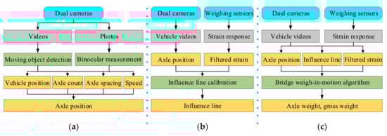
Figure 1.
Framework of the proposed BWIM: (a) binocular vision-based load localization; (b) load position-based influence line calibration; (c) load position-based axle weight estimation.
2.2. Automatic Recognizing and Positioning Vehicles and Wheels
In the proposed method, dual cameras were used to record a video of vehicles passing over the bridge to obtain the axle position for both the influence line calibration runs and vehicle weight identification runs. Automatic recognizing and positioning vehicles and axles (wheels) in three dimensions (3D) through the video was divided into three steps: (1) apply the moving object detection algorithm to quickly classify and accurately locate vehicles and wheels in every frame, and obtain the centroid pixel coordinates of the objects; (2) apply binocular ranging [32] and coordinate transformation [33] technology to obtain the 3D coordinates corresponding to each pixel of the frame; and (3) obtain the 3D coordinates of the objects according to the corresponding relationship between the pixel coordinate and the 3D coordinate.
2.2.1. Moving Object Detection
In this paper, a traditional computer vision (CV) algorithm and a deep learning (DL) algorithm were proposed for moving object detection. In the CV algorithm, the background difference method [34] was utilized for vehicle detection from video frames. After that, a circle detection method was utilized for wheel positioning in a single frame. Similar to former DL algorithms [35,36,37] which used a convolutional neural network (CNN) to automatically distinguish and accurately locate vehicles and wheels in video frames, the DL method in this paper was based on mask R-CNN [38].
The background difference method had four components: pre-processing, background modeling, foreground detection, and post-processing. The most critical component was the background modeling. In this paper, a Gaussian mixture model (GMM) [39] was used for background modeling, and was adaptable to complex environmental backgrounds and brightness changing. The circle detection method, a practical detection method based on edge shape characteristics of objects [8], was combined with the background difference method for vehicle and wheel detection.
Firstly, the background image was constructed based on all the video frames before the current image. Secondly, the current image was “subtracted” from the background image, and a proper thresholding was applied to the result to find the foreground image. Then, the contour image of the foreground was obtained by edge detection and morphological processing. Figure 2a shows one frame of a video recorded in a lab test. Figure 2b shows the obtained contour image. Finally, the bounding rectangle of the moving object based on foreground contour was obtained. In order to eliminate the influence of environmental changing on object detection, the background image was dynamically updated: the current image and the background image were compared pixel by pixel, and for each pixel, if the difference was less than a pre-set threshold, it was used to update the background; otherwise, it was considered as a foreground pixel. After the bounding box of the vehicle was roughly obtained, edge detection and Hough circle transform were carried out to detect the wheels in the bounding box. Figure 2c shows the detected edges, and Figure 2d shows the results of the identified moving vehicle and wheels.
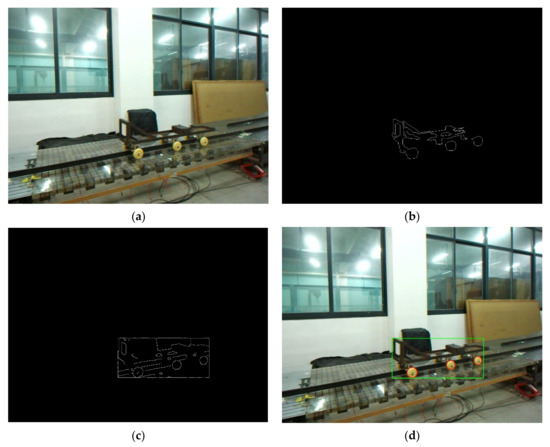
Figure 2.
Results of background difference method and circle detection: (a) recorded image; (b) foreground image contour; (c) detected edges in the bounding box; (d) identified vehicle and wheels.
An image recognition algorithm based on CNN is another type of moving object tracking method. In this paper, mask R-CNN was selected for vehicle and wheel detection. The schematic diagram of the algorithm is shown in Figure 3a. A whole recorded image was firstly inputted into a trained CNN (ResNet, etc.) for feature extraction. At the same time, the candidate regions of interest (RoIs) were generated by a region proposal network (RPN). After that, the RoIs were mapped to the last feature map of the CNN. Then, the last feature map was extracted by the RoIAlign layer to obtain fixed-size feature maps. Finally, these fixed-size feature maps were put into the mask branch and the classification and bounding box regression branch to generate the instance segmentation mask, class label, and bounding box of each candidate object. The position of the vehicle and wheel thus could be obtained from the center coordinates of the bounding box of the objects. Figure 3b shows the network-produced masks, and Figure 3c shows the class labels and bounding boxes of the identified moving vehicle and wheels.
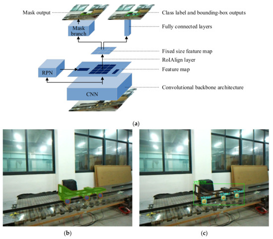
Figure 3.
Mask R-CNN: (a) framework of mask R-CNN for instance segmentation and object detection; (b) mask output; (c) class label and bounding box outputs.
2.2.2. Binocular Ranging and Coordinate Transformation
After obtaining the object’s centroid pixel coordinate via moving object detection, the corresponding relationship between the pixel coordinate and the 3D coordinate had to be determined in order to acquire the object’s 3D position. Binocular ranging and coordinate transformation technology can be used to implement the 3D coordinate transformation. The key processes are: binocular camera calibration, stereo rectification, stereo matching, and 3-D coordinate transformation.
The transformation relationship between the camera coordinate system O-X-Y-Z, the image coordinate system o-x-y, and the pixel coordinate system op-u-v can be constructed through the pinhole imaging model in Figure 4a and the similar triangle model in Figure 4b. Suppose there is a target point P (X, Y, Z) in the camera coordinate system. Among them, the image point of P in the imaging plane or pixel plane is P’; the image coordinate of the point P’ is (x, y); the pixel coordinate of the point P’ is (u, v); cx and cy are the offsets between the image coordinate system and pixel coordinate system along the x- and y-direction, respectively; f is the focal length of a single camera; and the distance from the target point P to the lens plane is the depth Z that can be obtained by binocular ranging technology.
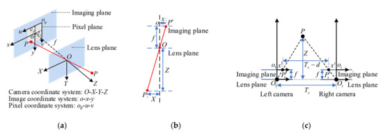
Figure 4.
Coordinate system transformation and binocular ranging: (a) pinhole imaging model; (b) similar triangle model; (c) principle of binocular ranging.
Generally, the relationship between the three coordinate systems can be derived based on the principle of triangular similarity, as shown in Equation (1):
where dx and dy are the physical lengths of a single pixel along the x- and y-direction, respectively; and K is the internal parameter matrix of a single camera. The unit of each parameter in K is pixels, and K can be obtained by via camera calibration.
The schematic diagram of measuring the depth Z with a binocular camera is shown in Figure 4c. In the figure, it was assumed that the cx, cy, and f of the left and right cameras were the same, which could ensure that the left and right imaging planes were completely aligned in parallel. The abscissa difference of the corresponding points Pl’ and Pr’ of the target point P on the two imaging planes had the following relationship relative to depth Z:
where d = xl−xr, xl and xr are the abscissas of the points Pl’ and Pr’ in the left and right image coordinate system, respectively; d is the abscissa difference of the target point P on the left and right imaging planes, namely disparity; and Tx is the center distance of the left and right cameras. From Equation (2), we obtained Z = fTx/d, which showed that as long as the disparity d of the target point P was measured, the depth Z could be obtained; then X, Y could be calculated by putting Z into Equation (1).
From the above analysis, in order to obtain the 3D coordinate of a point in the image, the parameters that needed to be obtained were f, cx, cy, Tx, and d. The binocular camera calibration could obtain the internal parameters (the internal parameter matrix K, the radial and tangential distortion coefficients) of each camera and the relative position of the two cameras (namely, the 3D translation parameter T (Tx, Ty, Tz) and rotation parameter R of the right camera relative to the left camera), so the initial values of f, cx, cy, and Tx could be calibrated. Stereo rectification eliminated the distortion of the left and right imaging planes through the internal parameters and the relative position of the two cameras, so that the f, cx, cy of the two cameras were the same, the optical axes of the two cameras were parallel, and the two imaging planes were coplanar. Stereo matching found the correspondence between the pixels of the two imaging planes based on stereo rectification to obtain the disparity map. Then, the depth information of the original image could be obtained through the disparity map. Finally, the 3-D coordinate transformation of the image could be estimated by via Equation (1).
In order to improve the efficiency of two-dimensional (2D) image matching in stereo matching, in this paper, the epipolar constraint was applied for image matching to effectively narrow search range and determine correct pixel correspondence. The epipolar constraint model of the binocular camera is shown in Figure 5a. The plane POlOr formed by the target point P and the optical centers Ol, Or of the two cameras is called the epipolar plane; the intersection points El, Er of the line OlOr and the two imaging planes are called epipolar points; and the intersection lines Pl’El, Pr’Er of the epipolar plane POlOr and the two imaging planes are called epipolar lines. The epipolar constraint could be obtained from the geometric relationship: the corresponding point Pr’ of a point Pl’ must lie in the epipolar line Pr’Er, and vice versa. This relationship reduced the image matching from a 2D search to a one-dimensional (1D) search, which improved the accuracy and speed of stereo matching.
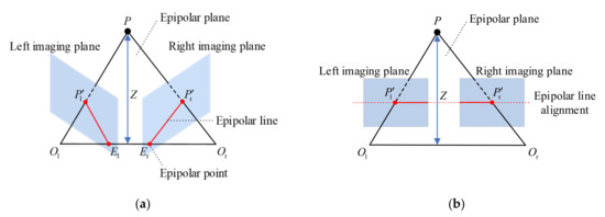
Figure 5.
Epipolar constraint models: (a) general epipolar constraint model; (b) epipolar constraint model after stereo rectification.
To further simplify the stereo matching process, stereo rectification is indispensable. As shown in Figure 5b, stereo rectification not only aligned the left and right imaging planes mathematically, but also completed the alignment of the epipolar line. At this time, the line OlOr was parallel to the two imaging planes, and the epipolar points El, Er were at infinity. After the epipolar line was aligned, the point Pl’ on the left imaging plane and the corresponding point Pr’ on the right imaging plane had the same line number, so the corresponding point Pr’ could be matched by a 1D search in this line, which made stereo matching more efficient.
2.3. Influence Line Calibration
O’Brien et al. [14] firstly proposed an efficient “matrix method” to automatically extract the influence line (IL) from the measured bridge response. The algorithm is very efficient, but is not applicable for non-constant cases since the load position the algorithm uses is calculated from speed and sampling time. Therefore, in this paper, the algorithm was re-derived by directly utilizing the axle position, instead of calculating from vehicle speed and sampling time.
When a calibration vehicle with known axle weights and axle spacing passes the bridge along lane l, the total strain response of the bridge at a certain bridge section can be measured. It can also be theoretically predicted:
where x is the position of the first axle of the calibration vehicle in the longitudinal direction; N is the number of axles; Pi is the weight of the i-th axle; Di is the distance between the i-th axle and the first axle; and is the ordinate value of IL at i-th axle’s position.
As shown in Figure 6, let the calibrating vehicle move a sufficiently small distance Δx forward from every sampling step. Let us say that from the moment the first axle reaches the entrance of the bridge until the last axle leaves the bridge exit, the total distance the vehicle has travelled is X. Then, there should be K steps sampled, where K = X/Δx + 1. Let and represent the measured and predicted response sampled at the k-th sampling step, respectively. Let represent the ordinate value of strain IL corresponding to the i-th axle at the k-th step, where Ci = Di/Δx. Then, the predicted response can be rewritten as , where and .
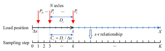
Figure 6.
Schematic diagram of data sampling.
It should be noted that data acquisition equipment usually works at a constant sampling frequency in the time domain rather than “constant distance Δx” in the x domain; therefore, a proper interpolation based on the monitored record load position–time (x–t) relationship may be needed to obtain the measured bridge response (k = 1,…,K).
Based on the least-squares method, the error function EIL was defined as the Euclidean distance between the measured bridge response and the theoretical one:
To minimize EIL, the ordinate value shall make the partial derivatives , therefore, we can obtain:
These equations can be expressed in matrix form:
where W (a sparse symmetric matrix), , and are:
By solving Equation (6), the IL ordinate vector can be obtained:
For a bridge with multiple lanes, the influence line of each lane can be obtained by simply repeating the proposed influence line calibration process with calibrating vehicle running in each lane.
2.4. Vehicle Weight Identification
In order to overcome the limitation of the constant speed assumption of the conventional BWIM algorithms, in this study, a new BWIM algorithm that identified the axle weight of multiple vehicles by matching the bridge response and axle loads with real position was proposed.
The bridge response predicted at the K sampling steps under a moving vehicle can be written in matrix form:
where , , and .
When multiple vehicles pass over the bridge, the total theoretical strain response will be:
where M is the count number of all the vehicles on the bridge. It should be noted that the matrix Lm in Equation (12) is calculated from the influence line of the lane the m-th vehicle running at and the actual axle load position of the m-th vehicle. Equation (12) can be rewritten as .
Like influence line calibration, the error function can be constructed based on the calibrated influence lines and the to-be-determined axle weights:
where . Apparently, as long as the number of sampling steps K is not less than the total number of axle count of all the vehicles, the axle weight vector P can be determined using the least-squares method:
After the weight vector P for the axles of all the vehicles is obtained, the gross vehicle weight (GVW) of each vehicle can be determined simply by summing the axle weights of the vehicle.
3. Experimental Setup
A series of laboratory scale-model tests were conducted to evaluate the performance of the proposed method. The test platform consisted of five parts: acceleration ramp, acceleration approach, bridge model, deacceleration approach, and deacceleration ramp, as shown in Figure 7a,b. The bridge had a width of 1.01 m and a length of 2.38 m, and was made with polymethyl methacrylate (PMMA) material. A cross section of the bridge is shown in Figure 7c. The Young’s modulus was 2795 MPa, and the density was 1181.6 kg/m3. More details of the test platform can be found in [40]. Two vehicle models, as shown in Figure 7d, were constructed for the experiments. It should also be noted that the spacing of the vehicle axles could be adjusted manually, and the weight of the vehicles could be changed by adding or removing mass blocks to/from the vehicles. The details of axle configurations (axle spacings and weights) of the vehicles for both calibration and tests are summarized in Table 1.
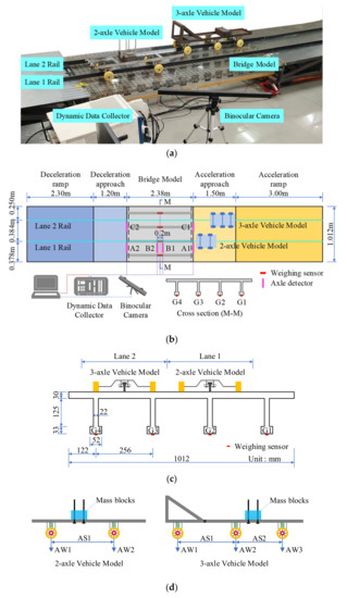
Figure 7.
Experimental platform: (a) actual scene; (b) schematic diagram; (c) cross section (M-M) of the bridge model; (d) vehicle models.

Table 1.
Axle spacings and weights of the vehicle models.
Two T-shaped rails were mounted on the platform to laterally force the vehicles to travel along the lanes. The lateral position of the rails was also adjustable. The initial speed of the vehicles was controlled by releasing the vehicle at a set height on the acceleration ramp. The height of all the supports of the five parts were individually adjustable. By adjusting the heights of the platform to form a slop road, the vehicles could be controlled to run at a constant or non-constant speed. Furthermore, to simulate a randomly changed speed (sudden acceleration or deacceleration), we directly dragged the vehicle by hand.
Four foil strain gauges (numbers G1 to G4, self-temperature compensated strain gauges, 3 mm × 5 mm) used to measure the global response of the bridge were attached under the soffit of the bridge girders and connected to a data acquisition equipment (an NI PXIe-1082 containing an NI PXIe-4331 module and an NI PXIe-8135 controller; sampling rate of 1000 Hz for vehicle speeds of 1 m/s~3 m/s), as shown in Figure 7a,b. These gauges were so-called “weighing sensors”. Two foil strain gauges were placed at the entrance and exit of each of the two lanes (positions A1, A2 and C1, C2) to monitor the time when a vehicle entered and left the bridge. Then, the average speed of the vehicle and its axle spacings could be calculated. These gauges were thus conventionally called “axle detectors”. Another two strain gauges were closely placed at positions B1 and B2 (with a distance of 0.2 m) to simulate another widely used axle-detecting configuration that monitored the instant speed of the vehicle while passing the mid-span of the bridge. In addition, in this study of binocular-vision-based vehicle locating, a hardware-integrated binocular camera was used to track the vehicles during the entire period from the moment they entered the bridge to the moment they left the bridge under normal light conditions. The baseline of the dual cameras was 334 mm. The resolution was 2560 × 960, and the sampling rate was 60 frames per second.
4. Results and Discussion
4.1. Comparison of the Moving Object Detection Algorithms
In order to comprehensively compare the efficiency and robustness of the CV method (based on background difference calculation and circle detection) and the DL method (based on mask R-CNN) on the vehicle and wheel detection, the three-axle vehicle shown in Figure 7d was set to run through the bridge and was recorded by the dual cameras. In the experiment, the cameras were installed to capture the vehicles at different shooting angles. The deflection angle between the camera lens plane and the longitudinal direction of the bridge was set to be about 0° (no deflection), 15° degrees (slight deflection), and 30° (deflection). It should be noted that the bridge deck was made of transparent PMMA and could reflect the vehicles in certain scenarios. For these tests, it was found that reflections could be captured when the deflection angle was about 30°. In real field tests, reflections may occur due to water on the bridge surface, and shadows may appear due to sunlight. Therefore, in this paper, the influence of the unexpected reflections on the performance of vehicle and wheel detection was also studied.
The vehicle tracking results of the two methods under different scenarios are summarized in Table 2. In the table, the recall rate of object detection is the ratio of the number of frames in which the vehicle or wheel was successfully identified to the total number of frames. It can be seen in the table that the DL method could correctly recognize the vehicle in most frames. The DL method based on mask R-CNN obtained the vehicle positions for all the frames, especially when the camera was not largely deflected (deflection angle close to or less than 15°). The CV method also worked very well for most tests, even with a 30° camera deflection angle. However, for the situations with the disturbance of reflections, the recall rate of vehicle detection decreased by more than 7%. For vehicle wheel detection, both of the methods performed great when the deflection angle was not larger than 15°. When the camera was deflected to 30°, the recall rates of the DL method were still greater than 98%, showing a good reliability in vehicle wheel recognition. The CV method performed worse in this section. This was because the CV method was based on a circle detection method. Larger deflection angle made the images of wheels in the camera-captured photos appear to be ellipses rather than standard circles. This drawback of the CV method could theoretically be conquered by using a more advanced ellipse detection method or by adding an image deflection correction step before circle detection in future studies. It should be pointed out that the CV method took less than 0.18 s on an Intel i5 CPU for one frame prediction, and the DL method took more than 1.8 s. Therefore, the CV method had a much better computational efficiency than the DL method, and computation speed usually is very important for real-time applications.
Table 2.
Object detection performance of the two methods.
It should also be noted that it was not necessary to conduct wheel detection for all frames. Instead, to determine the axle spacing of a vehicle, only a single frame was needed, or at most a few more frames for re-computation and confirmation. Table 3 shows the mean value and standard deviation (SD) of the relative errors of the axle spacing identification results. It can be seen from the table that the identification errors increased with the increase in the camera deflection angle. The reflection also seemed to have a negative influence on the axle spacing detection. However, the axle spacings were obtained with a good accuracy, since all the mean values were close to zero, and the standard deviations were all less than 4%. In addition, unlike the detection of vehicle and wheel positions, the identification errors of the CV method on axle spacing detection did not need to be greater than those of the DL method.
Table 3.
Axle spacing identification performance of the two methods.
Overall, both methods performed well in vehicle and wheel detection in this study. The following sections will show that the results for the vehicle positions and axle spacings met the requirement of axle weight identification. Apparently, the DL method had a better accuracy, and thus is a competitive alternative for vehicle and wheel detection in the future. In the meantime, the CV method is still an applicable option for traffic object detection in real BWIM systems due to its efficiency and the tolerance of the latest BWIM algorithms.
4.2. Vehicle Position Tracking
Figure 8 shows the 3D spatial positions (including velocity information) of the vehicle’s first axle in the camera coordinate system during the tests and the longitudinal locations of the vehicle’s first axle relative to time for several typical traffic scenes (such as slow deceleration, sudden acceleration, vehicle following, and parallel driving). In the spatial position figures, the sparseness of the vehicle trajectory points reflected the position change of the vehicle; namely, the sparser the trajectory points, the faster the vehicle moved. In the longitudinal location figures, the time histories of the data acquired from the axle detectors (strain sensors placed on the bridge deck surface) were also plotted for comparison purposes. The peaks on the curves indicated the time that the axles of the vehicle reached the axle detectors. The times when the vehicle’s first axle reached the axle detectors were interpolated from the location–time curve obtained from the camera-captured frames and are marked in the figures as well. It was found that the time of the vehicle’s first axle reach the axle detectors obtained from camera and axle detectors were basically consistent, which proved that the vision-based axle detection methods in this study were capable of obtaining reliable real-time locations of vehicle axles for BWIM usage. Furthermore, the methods could detect multiple vehicle objects at the same time, thus laying a foundation for a BWIM system to estimate axle and gross weight of vehicles for multiple vehicle presence.
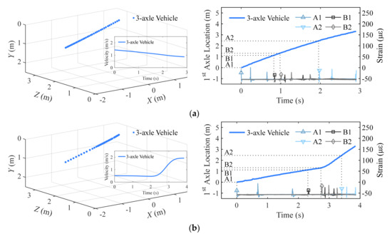
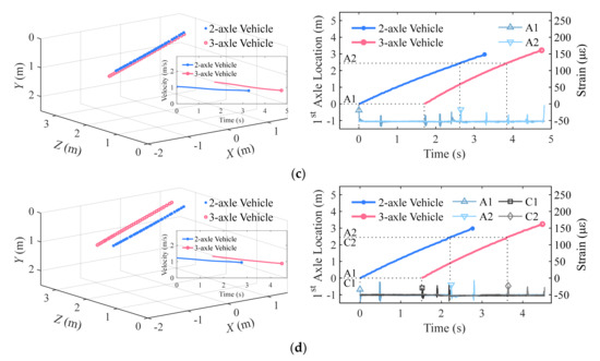
Figure 8.
The 3D spatial position and longitudinal location of vehicles: (a) slow deceleration; (b) sudden acceleration; (c) vehicle following; (d) parallel driving.
4.3. Influence Line Calibration under Non-Constant Velocity
Before the process of axle weight identification, the influence line (IL) should be calibrated. In the calibration tests of this study, a calibration vehicle (three-axle vehicle) with known axle weights and axle spacing was set to pass over the bridge along the center of each of the lanes in a range of speeds (1 m/s~3 m/s). During the tests, videos were shot and the data of weighing sensors (strain gauges installed under the soffit of bridge girders) were collected. The strain signals obtained from weighing sensors were then low-pass filtered by using simple Fourier transform (FFT) and inverse Fourier transform with a cut-off frequency at 10 Hz to remove the dynamic fluctuations and noise in the bridge strain response. The filtered strain response was finally used to extract the influence line.
To calculate the influence line, the position of the vehicle and its axles had to be determined. In the study, the axle position was obtained by using the proposed binocular-vision-based load-locating method (see Figure 1a). In addition, the vehicle position is conventionally computed from speed identified by using axle detectors based on constant velocity assumption. For comparison, two configurations of axle detectors, referred to as TRAD-1 and TRAD-2, were used. In the TRAD-1 scheme, two strain gages marked A1 and A2 (see Figure 7b) were placed at the entrance and the exit of the bridge. In the TRAD-2 scheme, two strain gages marked B1 and B2 (see Figure 7b) were placed in the middle of the bridge with a distance of 0.2 m. The vehicle positions (represented using the first axle) calculated using the three methods are plotted in Figure 9a, in which it can be seen that differences existed in the axle positions obtained using the three methods. The reason was that, due to inevitable frictional resistance between the vehicle wheels and the bridge model, the calibration vehicle could not always maintain a constant speed, and could slowly decelerates. It should be noted that, although the vehicle was intended to run at an absolute constant speed in the calibrating test, it was highly possible for certain fluctuations to occur in the real velocity of the vehicle, either significant or tiny.
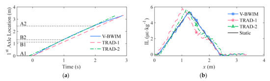
Figure 9.
Influence line calibration: (a) identified axle position; (b) influence line calibrated from different methods.
Figure 9b shows the influence line extracted from the bridge response under the vehicle load by using the previously obtained vehicle positions. The influence line measured by single static load is also plotted in the figure. In Figure 9b, the abscissa of the influence line is the load position (x, unit: m), and the ordinate is the influence line value (IL, unit: με∙kg−1). “TRAD-1” and “TRAD-2” refer to influence lines calibrated using the vehicle positions calculated from the installed axle detectors, respectively. “Static” refers to the statically measured influence line. To quantitatively analyze the influence line results calibrated using the proposed method and the traditional method, Table 4 shows the detailed identification errors for eight calibration runs. In Table 4, v0 and vend indicate the speed of the vehicle at the time it entered the bridge and the speed at which it left the bridge, respectively; Δv indicates the relative difference between the two speeds; and MSE indicates mean-square error between the calibrated influence line and the static influence line.
Table 4.
Identification errors of the calibrated IL (lane 1).
It was found from the figure that the influence lines calculated using the traditional method, with the TRAD-1 or TRAD-2 scheme, were not consistent to the static IL. Specially, the highest peak of the TRAD-1 and TRAD-2 curves were obviously prior to the peak of the static IL. This was because the axle detectors could not provide the accurate axle position for the entire test period. On the contrary, the IL calculated using V-BWIM methods fit the static IL very well, no matter the IL curve shape, the peak location, or the peak height. This indicated that the IL could be accurately acquired by the proposed method.
From the detailed results stated in Table 4, it was further revealed that the mean-square error of the traditional methods increased with the increase of the speed difference; while for the considered eight tests or similar scenarios, the MSE of the proposed V-BWIM method remained steady and was significant smaller than that of the traditional methods. Apparently, the negative impact of a non-constant speed on the accuracy of IL calibration could be effectively suppressed by the proposed method, which again proved that the accuracy of the identified vehicle position had an important influence on the IL calibration, and the proposed vision-based, whole-period vehicle-position monitoring technique was necessary for IL calibration use and future BWIM applications. Moreover, for real applications in which traditional axle detectors are the option, it seems TRAD-2 may be a more reasonable axle-detector scheme (sensors were installed close to the midspan) than TRAD-1 due to its better performance, since the predicted axle position using the TRAD-2 scheme was closer to the real position than that of the TRAD-1 scheme.
Based on the proposed method, the influence line of each of the two lanes was calibrated and averaged from eight independent tests to reduce the effect of dynamic vibration and measurement noise, as shown in Figure 10.
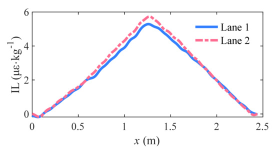
Figure 10.
Calibrated influence line (averaged from 8 ILs).
4.4. Vehicle Weight Identification under Non-Constant Velocity
It was obvious that a similar accuracy would be achieved using the proposed method and the traditional axle-detector-based method for a situation in which the vehicle ran at a constant speed; thus, only non-constant scenarios were conducted in this section to evaluate the advantages of the proposed method. In the non-constant-velocity tests, a three-axle vehicle was used to simulate four types of typical driving behavior: VS-I (vehicle accelerates at 1/2 span), VS-II (vehicle decelerates at 1/2 span), VS-III (vehicle accelerates at 1/4 span and decelerates at 3/4 span), and VS-IV (vehicle decelerates at 1/2 span until stopping, and then accelerates to leave the bridge). For each testing mode, eight independent tests were performed. In addition, in order to compare the traditional vehicle weight identification method with the proposed method, the axle detectors (A1 and A2) at the entrance and exit of the bridge and the axle detectors (B1 and B2) near the mid-span were used to detect the vehicle speed for the vehicle weight identification of the traditional method.
For illustration purposes, Figure 11 shows the measured bridge strain of one of the eight tests for each of four driving scenarios, respectively. The results of vehicle tracking are also plotted in the figure. Stars on the vehicle position curve indicate where the vehicle changed its speed. The original bridge strain was filtered, and then was used by the proposed V-BWIM method to obtain the axle weight of the vehicle. The reconstructed strains based on the identified weight and IL for the tests are also plotted in Figure 11. To evaluate the extent of accordance between the reconstructed strain and the source strain (filtered), a ratio r2 of the norm of difference between the two strain curves to the norm of the source strain was introduced; the formula of r2 is shown as follows:
where y is the vector of the source strain (filtered), and y′ is the vector of the reconstructed strain. Apparently, r indicates the relative vector error between the two strain vectors.
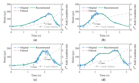
Figure 11.
Bridge strain and identified vehicle position (non-constant velocity): (a) VS-I: vehicle accelerates at 1/2 span; (b) VS-II: vehicle decelerates at 1/2 span; (c) VS-III: vehicle accelerates at 1/4 span and decelerates at 3/4 span; (d) VS-IV: vehicle decelerates at 1/2 span until stopping, and then accelerates to leave the bridge.
The relative vehicle weight identification errors and the relative vector errors r of the proposed method are summarized in Table 5. The relative vehicle weight identification errors of the traditional axle-detector-based methods are summarized in Table 6 and Table 7. TRAD-1 and TRAD-2 indicate the relative errors by using the traditional method with the two schemes of axle detector installations (A1 and A2, B1 and B2), respectively. In the table, mean and SD refer to the average value and standard deviation of the relative errors of the eight tests for each driving scenario.
Table 5.
Vehicle weight identification errors of V-BWIM.
Table 6.
Vehicle weight identification errors of TRAD-1.
Table 7.
Vehicle weight identification errors of TRAD-2.
From Table 6 and Table 7, it is easy to see that the results of the traditional method (for both of the two axle-detector schemes) were not reliable under the considered non-constant velocity situations. On the contrary, as shown in Table 5, all the errors of the proposed method were successfully controlled to be less than 2.5% for gross weight identification, and the axle weight errors did not exceed 6.5%. In Figure 11, it can be seen that the reconstructed strain and the source strain (filtered) were in a very good accordance (the relative vector error r for all tests was below 4%). Overall, we concluded that the proposed method could accurately identify axle weights of a vehicle even it passed over the instrumented bridge at a non-constant velocity.
4.5. Vehicle Weight Identification for Multiple Vehicle Presence
Another advantage of using traffic surveillance cameras is that all the vehicles on the test bridge could be captured and effectively tracked at the same time. Therefore, the proposed method has a good potential ability to properly deal with the multiple vehicle presence problem of BWIM systems. In order to verify the effectiveness of the method on multi-vehicle weight identification, two typical traffic scenes were simulated: two vehicles (a two-axle vehicle and a three-axle vehicle) following one by one (M-I), and the two vehicles running in parallel lanes (M-II, two-axle vehicle in the left lane and three-axle vehicle in the right lane). The experiment was independently repeated eight times to reduce the effects of randomness. During the tests, the inevitable friction again made the vehicles slowly decelerate.
As in the single-vehicle tests, the bridge strain response was measured and filtered, and the vehicle position was tracked, as shown in Figure 12, for the proposed method to detect the vehicle axle weight. The errors of the identified weight of the two vehicles by the proposed method are illustrated in Table 8. Mean and SD refer to the average value and standard deviation of the relative error of the eight tests for each driving scenario. In addition, for comparison purposes, the axle detectors (A1, A2 and C1, C2) at the entrance and exit of each of the two lanes were used to detect the number of axles and vehicle speed as well for vehicle weight identification by using the traditional axle-detector-based method. The relative errors of the identification results for the traditional method are shown in Table 9.
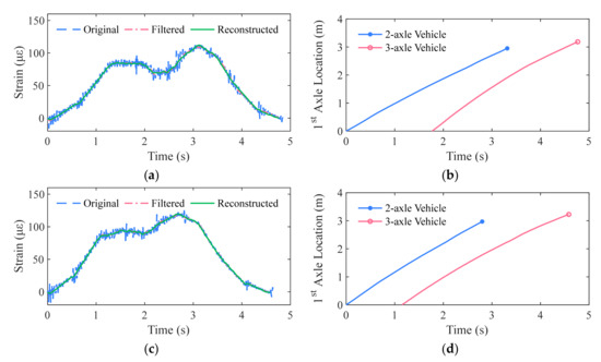
Figure 12.
Bridge strain and identified vehicle position (multiple vehicle presence): (a) M-I: vehicle following, bridge strain; (b) M-I: vehicle following, vehicle positions; (c) M-II: parallel driving, bridge strain; (d) M-II: parallel driving, vehicle positions.
Table 8.
Vehicle weight identification errors of V-BWIM.
Table 9.
Vehicle Weight identification errors of the traditional method.
It can be seen in Table 8 that all the relative gross vehicle weight errors were less than 3%, and the axle weight errors also did not exceed 6%. In Figure 12, it can also be seen that the reconstructed strain based on the identified weight and IL were very close to the source strain (filtered). In addition, it can be seen in Table 9 that the gross vehicle weight (GVW) of each of the two vehicles was obtained by the traditional method with a worse accuracy relative to V-BWIM method, but was still acceptable: most of them were smaller than 5%, and all of them were no more than 6.2%. However, the axle weight error dramatically grew to not less than 20%, which was multiple times larger than that of the V-BWIM method. Namely, even for a slight speed change, while the identified GVW result may not be significantly affected, unignorable errors could be imported in axle weight identification. This proved that the traditional method based on constant speed consumption is highly sensitive to the quality of the result of vehicle speed monitoring. Therefore, a reliable vehicle positioning method is crucial for ensuring the effectiveness of vehicle weight identification. Considering the performance of the proposed method on the considered tests, we concluded that the new V-BWIM method can be a competitive alternative for multiple vehicle weight monitoring.
5. Conclusions
Vehicles can travel at variable speeds when crossing a bridge. Due to this, traditional BWIM techniques cannot accurately match the position of the vehicles on the bridge with the bridge response, leading to errors in vehicle weight identification. This paper proposed a new strategy of the BWIM technique that consisted of three parts: the binocular-vision-based vehicle-locating method, the real-position-based influence line calibration method, and the real-position-based axle weight identification method. Laboratory experiments with scaled vehicle and bridge models were conducted to evaluate the performance of proposed method. Based on the test results, the following conclusions were reached:
- (1)
- For moving vehicle tracking, the deep learning (DL) method based on mask R-CNN had a better accuracy, but the conventional CV method was more efficient. Regarding axle spacing identification, there was no significant difference between the two methods. Generally, both methods could fulfill the requirements of a BWIM system based on the need of vehicle load position identification. In future practical applications, it would be worth combining the two methods to obtain a faster and more accurate vehicle-tracking method.
- (2)
- A slight change of vehicle speed can induce remarkable errors in the influence line calibration results for conventional BWIM methods that are based on constant speed assumption. Test results showed that a larger change of speed caused larger errors, while the mean-square errors of the influence line extracted by the proposed V-BWIM method for all the considered varying speeds were similar, and were 10 times smaller than those of the conventional method. Namely, the proposed method could accurately estimate the bridge influence line despite speed changes during the calibration process.
- (3)
- The largest relative errors of identified axle weight and gross vehicle weight by using the V-BWIM method were 6.18% and 2.23%, respectively, for all single-vehicle-presence tests in which the vehicle ran at a non-constant speed. In contrast, those errors of the conventional method could exceed tens, and even hundreds of percent. The reason for this was mainly because the V-BWIM method constructed the objective function based on the correct relationship between axle load positions and bridge response, while the axle position information that the conventional method used was calculated from vehicle speed and axle spacing, which was not consistent with the real position under the circumstances in which the vehicle did not run at a constant speed. Thus, obtaining accurate load positions and providing them to a BWIM system is vital for axle weight identification.
- (4)
- For a multi-presence scenario in which two vehicles were passing over the test bridge one by one or side by side, the axle and gross weight of the vehicles was successfully obtained, with axle weight errors less than 6% and gross weight errors less than 3%. It also outperformed the traditional method, which, in the conducted slow-deceleration tests, the gross weight error was still controlled within 7%, but the axle weight error was vast and unacceptable.
The main advantage of the proposed V-BWIM method is that the vehicle position at every moment during the period the vehicle passes over the bridge is tracked, and the axle weight then can be accurately obtained. However, these conclusions were made based on laboratory tests. In future studies, field tests should be conducted to verify the effectiveness of the method in real-world scenarios. Moreover, the computational efficiency of the object-locating algorithm based on dual camera vision used in this paper should be improved for real-time applications in the future. It should also be noted that the proposed V-BWIM method was only verified in a laboratory with normal brightness and stable camera system. For real applications under unfavorable conditions such as low light and extreme weather, necessary measures such as additional illumination or a pre-defogging process should be adopted to prevent failure.
Author Contributions
Conceptualization, D.Z. and W.H.; methodology, D.Z.; software, D.Z., L.D. and H.X.; validation, W.H., Y.W. and J.D.; formal analysis, D.Z. and W.H.; investigation, D.Z., H.X. and J.D.; resources, W.H. and L.D.; data curation, D.Z., H.X. and J.D.; writing—original draft preparation, D.Z. and Y.W.; writing—review and editing, W.H., L.D. and Y.W.; visualization, D.Z., H.X. and J.D.; supervision, W.H. and L.D.; project administration, W.H.; funding acquisition, W.H. and L.D. All authors have read and agreed to the published version of the manuscript.
Funding
This research was funded by the National Natural Science Foundation of China (grant nos. 52108139 and 51778222), the Key Research and Development Program of Hunan Province of China (grant no. 2017SK2224), and the Hunan Province funding for leading scientific and technological innovation talents (grant no. 2021RC4025).
Conflicts of Interest
The authors declare no conflict of interest.
References
- Deng, L.; Wang, T.; He, Y.; Kong, X.; Dan, D.; Bi, T. Impact of Vehicle Axle Load Limit on Reliability and Strengthening Cost of Reinforced Concrete Bridges. China J. Highw. Transp. 2020, 33, 92–100. [Google Scholar]
- Richardson, J.; Jones, S.; Brown, A.; O’Brien, E.J.; Hajializadeh, D. On the use of bridge weigh-in-motion for overweight truck enforcement. Int. J. Heavy Veh. Syst. 2014, 21, 83–104. [Google Scholar] [CrossRef]
- Yu, Y.; Cai, C.S.; Deng, L. State-of-the-art review on bridge weigh-in-motion technology. Adv. Struct. Eng. 2016, 19, 1514–1530. [Google Scholar] [CrossRef]
- Algohi, B.; Bakht, B.; Khalid, H.; Mufti, A.; Regehr, J. Some observations on BWIM data collected in Manitoba. Can. J. Civ. Eng. 2020, 47, 88–95. [Google Scholar] [CrossRef]
- Algohi, B.; Mufti, A.; Bakht, B. BWIM with constant and variable velocity: Theoretical derivation. J. Civ. Struct. Health 2020, 10, 153–164. [Google Scholar] [CrossRef]
- Cantero, D. Moving point load approximation from bridge response signals and its application to bridge Weigh-in-Motion. Eng. Struct. 2021, 233, 111931. [Google Scholar] [CrossRef]
- Brouste, A. Testing the accuracy of WIM systems: Application to a B-WIM case. Measurement 2021, 185, 110068. [Google Scholar] [CrossRef]
- Ye, X.; Dong, C. Review of Computer Vision-based Structural Displacement Monitoring. China J. Highw. Transp. 2019, 32, 21–39. [Google Scholar]
- Pieraccini, M.; Miccinesi, L. An Interferometric MIMO Radar for Bridge Monitoring. IEEE Geosci. Remote Sens. Lett. 2019, 16, 1383–1387. [Google Scholar] [CrossRef]
- Miccinesi, L.; Consumi, T.; Beni, A.; Pieraccini, M. W-band MIMO GB-SAR for Bridge Testing/Monitoring. Electronics 2021, 10, 2261. [Google Scholar] [CrossRef]
- Tosti, F.; Gagliardi, V.; D’Amico, F.; Alani, A.M. Transport infrastructure monitoring by data fusion of GPR and SAR imagery information. Transp. Res. Proc. 2020, 45, 771–778. [Google Scholar] [CrossRef]
- Lazecky, M.; Hlavacova, I.; Bakon, M.; Sousa, J.J.; Perissin, D.; Patricio, G. Bridge Displacements Monitoring Using Space-Borne X-Band SAR Interferometry. IEEE J. Sel. Top. Appl. Earth Obs. Remote. Sens. 2017, 10, 205–210. [Google Scholar] [CrossRef] [Green Version]
- Moses, F. Weigh-in-motion system using instrumented bridges. Transp. Eng. J. 1979, 105, 233–249. [Google Scholar] [CrossRef]
- O’Brien, E.J.; Quilligan, M.J.; Karoumi, R. Calculating an influence line from direct measurements. Proc. Inst. Civ. Eng.-Br. 2006, 159, 31–34. [Google Scholar] [CrossRef]
- Ieng, S.S. Bridge Influence Line Estimation for Bridge Weigh-in-Motion System. J. Comput. Civ. Eng. 2015, 29, 06014006. [Google Scholar] [CrossRef]
- Jacob, B. Weighing-in-Motion of Axles and Vehicles for Europe (WAVE). Rep. of Work Package 1.2; Laboratoire Central des Ponts et Chaussées: Paris, France, 2001. [Google Scholar]
- Lansdell, A.; Song, W.; Dixon, B. Development and testing of a bridge weigh-in-motion method considering nonconstant vehicle speed. Eng. Struct. 2017, 152, 709–726. [Google Scholar] [CrossRef]
- Zhuo, Y. Application of Non-Constant Speed Algorithm in Bridge Weigh-in-Motion System. Master’s Thesis, Hunan University, Changsha, China, 2015. (In Chinese). [Google Scholar]
- Chen, Z.; Li, H.; Bao, Y.; Li, N.; Jin, Y. Identification of spatio-temporal distribution of vehicle loads on long-span bridges using computer vision technology. Struct. Control Health Monit. 2016, 23, 517–534. [Google Scholar] [CrossRef]
- Khuc, T.; Catbas, F.N. Structural Identification Using Computer Vision–Based Bridge Health Monitoring. J. Struct. Eng. 2018, 144, 04017202. [Google Scholar] [CrossRef]
- Zhu, J.; Li, X.; Zhang, C.; Shi, T. An accurate approach for obtaining spatiotemporal information of vehicle loads on bridges based on 3D bounding box reconstruction with computer vision. Measurement 2021, 181, 109657. [Google Scholar] [CrossRef]
- Ojio, T.; Carey, C.H.; O’Brien, E.J.; Doherty, C.; Taylor, S.E. Contactless Bridge Weigh-in-Motion. J. Bridge Eng. 2016, 21, 04016032. [Google Scholar] [CrossRef] [Green Version]
- Zhang, B.; Zhou, L.; Zhang, J. A methodology for obtaining spatiotemporal information of the vehicles on bridges based on computer vision. Comput.-Aided Civ. Inf. 2019, 34, 471–487. [Google Scholar] [CrossRef]
- Dan, D.; Ge, L.; Yan, X. Identification of moving loads based on the information fusion of weigh-in-motion system and multiple camera machine vision. Measurement 2019, 144, 155–166. [Google Scholar] [CrossRef]
- Ge, L.; Dan, D.; Li, H. An accurate and robust monitoring method of full-bridge traffic load distribution based on YOLO-v3 machine vision. Struct. Control Health Monit. 2020, 27, e2636. [Google Scholar] [CrossRef]
- Xia, Y.; Jian, X.; Yan, B.; Su, D. Infrastructure Safety Oriented Traffic Load Monitoring Using Multi-Sensor and Single Camera for Short and Medium Span Bridges. Remote Sens. 2019, 11, 2651. [Google Scholar] [CrossRef] [Green Version]
- Zhou, Y.; Pei, Y.; Li, Z.; Fang, L.; Zhao, Y.; Yi, W. Vehicle weight identification system for spatiotemporal load distribution on bridges based on non-contact machine vision technology and deep learning algorithms. Measurement 2020, 159, 107801. [Google Scholar] [CrossRef]
- Quilligan, M.; Karoumi, R.; O’Brien, E.J. Development and Testing of a 2-Dimensional Multi-Vehicle Bridge-WIM Algorithm. In Proceedings of the 3rd International Conference on Weigh-in-Motion (ICWIM3), Orlando, FL, USA, 13–15 May 2002; Wiley: New York, NY, USA, 2002. [Google Scholar]
- Zhao, H.; Uddin, N.; O’Brien, E.J.; Shao, X.; Zhu, P. Identification of Vehicular Axle Weights with a Bridge Weigh-in-Motion System Considering Transverse Distribution of Wheel Loads. J. Bridge Eng. 2014, 19, 04013008. [Google Scholar] [CrossRef] [Green Version]
- Chen, S.Z.; Wu, G.; Feng, D.C. Development of a bridge weigh-in-motion method considering the presence of multiple vehicles. Eng. Struct. 2019, 191, 724–739. [Google Scholar] [CrossRef]
- Liu, Y. Study on the BWIM Algorithm of A Vehicle or Multi-Vehicles Based on the Moses Algorithm. Master’s Thesis, Jilin University, Changchun, China, 2019. (In Chinese). [Google Scholar]
- Marr, D.; Poggio, T. Cooperative Computation of Stereo Disparity. Science 1976, 194, 283–287. [Google Scholar] [CrossRef] [Green Version]
- Wang, Y.J. Displacement Measurement Method of Sphere Joints Based on Machine Vision and Deep Learning. Master’s Thesis, Zhejiang University, Hangzhou, China, 2018. (In Chinese). [Google Scholar]
- Yang, B. The Research on Detection and Tracking Algorithm of Moving Target in Video Image Sequence. Master’s Thesis, Lanzhou University of Technology, Lanzhou, China, 2020. (In Chinese). [Google Scholar]
- Girshick, R.; Donahue, J.; Darrell, T.; Malik, J. Rich Feature Hierarchies for Accurate Object Detection and Semantic Segmentation. In Proceedings of the IEEE Conference on Computer Vision and Pattern Recognition, Columbus, OH, USA, 24–27 January 2014; pp. 580–587. [Google Scholar]
- Schmidhuber, J. Deep learning in neural networks: An overview. Neural Netw. 2015, 61, 85–117. [Google Scholar] [CrossRef] [PubMed] [Green Version]
- Ren, S.; He, K.; Girshick, R.; Sun, J. Faster R-CNN: Towards Real-Time Object Detection with Region Proposal Networks. IEEE Trans. Pattern Anal. 2017, 39, 1137–1149. [Google Scholar] [CrossRef] [PubMed] [Green Version]
- He, K.; Gkioxari, G.; Dollár, P.; Girshick, R. Mask R-CNN. In Proceedings of the IEEE International Conference on Computer Vision, Venice, Italy, 22–29 October 2017; pp. 2961–2969. [Google Scholar]
- Zhang, W.; Wu, Q.M.J.; Wang, G.; Yin, H. An Adaptive Computational Model for Salient Object Detection. IEEE Trans. Multimedia 2010, 12, 300–316. [Google Scholar] [CrossRef]
- He, W.; Ling, T.; O’Brien, E.J.; Deng, L. Virtual axle method for bridge weigh-in-motion systems requiring no axle detector. J. Bridge Eng. 2019, 24, 04019086. [Google Scholar] [CrossRef]
Publisher’s Note: MDPI stays neutral with regard to jurisdictional claims in published maps and institutional affiliations. |
© 2021 by the authors. Licensee MDPI, Basel, Switzerland. This article is an open access article distributed under the terms and conditions of the Creative Commons Attribution (CC BY) license (https://creativecommons.org/licenses/by/4.0/).