Abstract
Fine-resolution satellite imagery is needed for characterizing dry-season phenology in tropical forests since many tropical forests are very spatially heterogeneous due to their diverse species and environmental background. However, fine-resolution satellite imagery, such as Landsat, has a 16-day revisit cycle that makes it hard to obtain a high-quality vegetation index time series due to persistent clouds in tropical regions. To solve this challenge, this study explored the feasibility of employing a series of advanced technologies for reconstructing a high-quality Landsat time series from 2005 to 2009 for detecting dry-season phenology in tropical forests; Puerto Rico was selected as a testbed. We combined bidirectional reflectance distribution function (BRDF) correction, cloud and shadow screening, and contaminated pixel interpolation to process the raw Landsat time series and developed a thresholding method to extract 15 phenology metrics. The cloud-masked and gap-filled reconstructed images were tested with simulated clouds. In addition, the derived phenology metrics for grassland and forest in the tropical dry forest zone of Puerto Rico were evaluated with ground observations from PhenoCam data and field plots. Results show that clouds and cloud shadows are more accurately detected than the Landsat cloud quality assessment (QA) band, and that data gaps resulting from those clouds and shadows can be accurately reconstructed (R2 = 0.89). In the tropical dry forest zone, the detected phenology dates (such as greenup, browndown, and dry-season length) generally agree with the PhenoCam observations (R2 = 0.69), and Landsat-based phenology is better than MODIS-based phenology for modeling aboveground biomass and leaf area index collected in field plots (plot size is roughly equivalent to a 3 × 3 Landsat pixels). This study suggests that the Landsat time series can be used to characterize the dry-season phenology of tropical forests after careful processing, which will help to improve our understanding of vegetation–climate interactions at fine scales in tropical forests.
1. Introduction
Climate change is lengthening dry seasons in many tropical regions [1,2] and changing the vegetation phenology [3], and it is intensifying drought, heat, fires, storms, and flooding [1]. Forest fragmentation strengthens the impacts of these disturbances [4,5,6,7]. Tree mortality from drought, heat, and storms is increasing worldwide [8,9,10], particularly in more seasonal tropical forests and savannas [5,9,11]. These changes could cause tropical forests to change from a net sink to a net source of CO2 emissions [12], and together with other human pressures, pose major risks to Earth’s biodiversity [13,14]. Drought-related changes in the seasonal phenology of greenness patterns in satellite imagery, i.e., dry-season phenology, can yield insights into how tropical forests may respond to climate change [15,16,17,18].
In heterogeneous tropical landscapes, the high spatial resolution of Landsat images is needed for characterizing dry-season phenology with metrics such as dry-season start and end dates (browndown and greenup dates, respectively). The higher spatial resolution of Landsat has several advantages. First, tropical forest species composition and functional traits can change drastically over distances shorter than the 0.25- to 1-km pixels of high-frequency imagery such as MODIS. Geology, stand age, and topography, for example, affect stand deciduousness, leaf thickness, and basal area of nitrogen-fixing species [19]. Soil nitrogen and phosphorus also affect tropical forest functional traits [20,21]. Second, tree competition for light in models of forest dynamics, and related carbon cycling, is typically modeled at 15 to 20-m spatial scales [22,23,24]. Third, satellite imagery with fine spatial resolution should mitigate uncertainties in phenology detection. Recent studies have found that uncertainty in phenological start and end dates increases with pixel size [25,26]. In addition, the long record of Landsat images (over 40 years) can help reveal long-term change in the phenology of tropical regions. Landsat imagery has been demonstrated to be effective in detecting phenology over large temperate areas [27,28,29], for mapping tree species [30,31], for mapping forest habitats [32], and for mapping detailed types of agriculture in tropical zones [33,34,35]. However, Landsat imagery has rarely been used for characterizing tropical forest phenology and simultaneously filling cloud gaps over large areas encompassing multiple scenes. Possible reasons are the high frequency of cloudy days in tropical regions, which reduce the availability of cloud-free Landsat images, and the long revisit cycle of Landsat satellites (16 days), which worsens the cloud contamination issue. Fortunately, advanced technologies have been developed in the past decade for solving the impact of clouds on the applications of Landsat images, including automatic detection of clouds [36,37,38] and cloud removal [39,40]. Therefore, it is urgent to explore the potential of Landsat imagery for monitoring vegetation phenology in cloudy tropical regions with the aid of advanced image-processing technologies.
To solve these research challenges, this study develops an operational method to employ Landsat images to characterize the dry-season phenology of tropical dry forest in Puerto Rico. The developed method employs cutting-edge algorithms for automated cloud screening [36], missing data interpolation [39], and bidirectional reflectance distribution function (BRDF) correction [41], to reconstruct a high-quality Landsat time series. It then extracts 15 dry-season phenology metrics from the reconstructed enhanced vegetation index (EVI) time series through a robust phenology-detection method. Field plots and PhenoCam data were used to validate the results for the developed method. The innovation of this study is three-fold: (1) it tests the feasibility of phenology detection from Landsat time series in tropical regions, and the findings will facilitate studies of long-term changes in tropical phenology using Landsat historical data; (2) it introduces an operational framework to process Landsat images for phenology detection, which can be easily adopted by future studies since the codes have been made available to the public; and (3) it defines a comprehensive set of dry-season phenology metrics, which can better support the study of phenology–climate interactions. The rest of this paper is organized as follows: Section 2 describes the study area and data sets used, Section 3 introduces the details of steps employed for reconstructing Landsat time series data and the method for detecting and validating phenology metrics, Section 4 presents the results, Section 5 discusses the implications and limitations of our approach, and Section 6 concludes this study.
2. Study Area and Data Used
2.1. Study Area
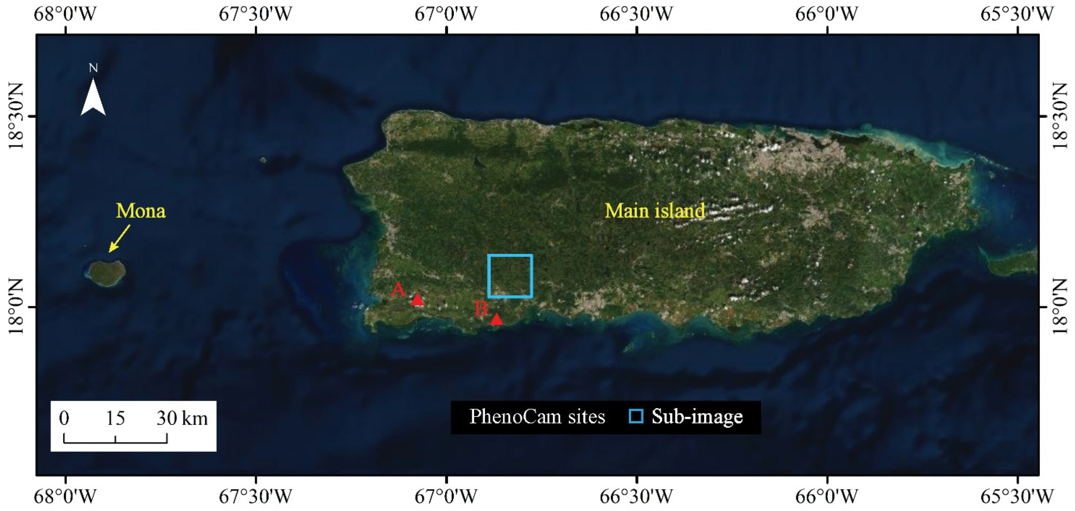
The study area includes the main island and Mona Island of the Commonwealth of Puerto Rico (Figure 1), which is a biologically diverse tropical region in the Caribbean Sea. Its spatial heterogeneity in vegetation biophysical attributes is largely due to a wide range of soil types, previous land use types, temperature, rainfall, and ground-level clouds. Soils have formed on alluvial, sedimentary, extrusive volcanic, limestone, and serpentine substrates, supporting forests with high tree species diversity. The most extensive climatic zone has broadleaf evergreen forest, but other forest types, including dry semi-deciduous forest and cloud forest, are present at significant extents. Cloud forests dominate the highest elevations, above the cloud condensation level. Cloud forests, forests on serpentine substrate, and some areas of forest on karst substrate have high proportions of sclerophyllous or microphyllous leaves [19].
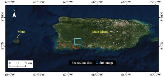
Figure 1.
Map of the study area showing the main island and Mona island of Puerto Rico, and the location of two PhenoCam sites and a sub-image that were used to validate the results of this study.
2.2. Data Used
This study used Landsat 7 ETM+ and Landsat 8 OLI Collection 1 Level-2 surface reflectance products, which were generated by U.S. Geological Survey (USGS). For these products, the USGS applies radiometric calibration and atmospheric correction algorithms to Level-1 Landsat data products. The visible and infrared bands of these sensors were used here, including the blue, green, red, near-infrared, and shortwave infrared bands. In addition, when choosing Landsat imagery, only images with less than 50% cloud cover over the land surface were selected to ensure that imagery had substantial clear observations.
This analysis included data from two time periods. First, it included Landsat 7 data from the years 2005 to 2009 to ensure enough cloud-free observations to compose a “one-year-like” seasonal time series for reliable phenology detection. Table 1 lists the day of year (DOY) of the Landsat 7 scenes used in this study to capture mainland Puerto Rico (54 images) and Mona Island (38 images). This period was chosen because it has no significant climate changes regarding temperature and precipitation, no extreme weather events occurred (e.g., cyclones, drought), and it corresponds to years surrounding the Mona Island forest inventory in the year 2008. We can derive a phenology product that represents an average situation in this 5-year window, assuming vegetation did not undergo much disturbance during this time. This strategy has been used in previous studies in cloudy regions, such as mapping bamboo phenology [31] and needle-leaf forest phenology [29]. Images were collected and ordered by DOY to compose a one-year time series. Second, it included 17 Landsat 8 OLI images from the years 2016–2017. This period was also chosen because it corresponded to a period with no significant climate events and when different kinds of ground-based validation data were available. This period was after a severe drought in 2015 and before Hurricane Maria in 2017. Our focus for this second time period is on phenocam data from mainland Puerto Rico dry zones, where sufficient cloud-free observations to estimate phenology metrics can be obtained with 2016–2017 Landsat images. Although Sentinel-2 imagery were available during that time, incorporating it into the framework we present here is a subject of ongoing research.

Table 1.
Day of year (DOY) of Landsat images used in this study over Mona Island and main island of Puerto Rico.
To validate the phenology metrics derived by the proposed method, we used forest inventory data and PhenoCam data from the tropical dry forest zone of Puerto Rico, including in Southwestern Puerto Rico and on Mona Island. Forest inventory data were from the U.S. Department of Agriculture Forest Service, Forest Inventory, and Analysis program (FIA), which is jointly implemented in Puerto Rico by the Southern Research Station and the International Institute of Tropical Forestry. The PhenoCam data were collected from 2 sites in Puerto Rico (Figure 1) from the PhenoCam network (https://PhenoCam.us/, accessed on 1 September 2021).
3. Methods
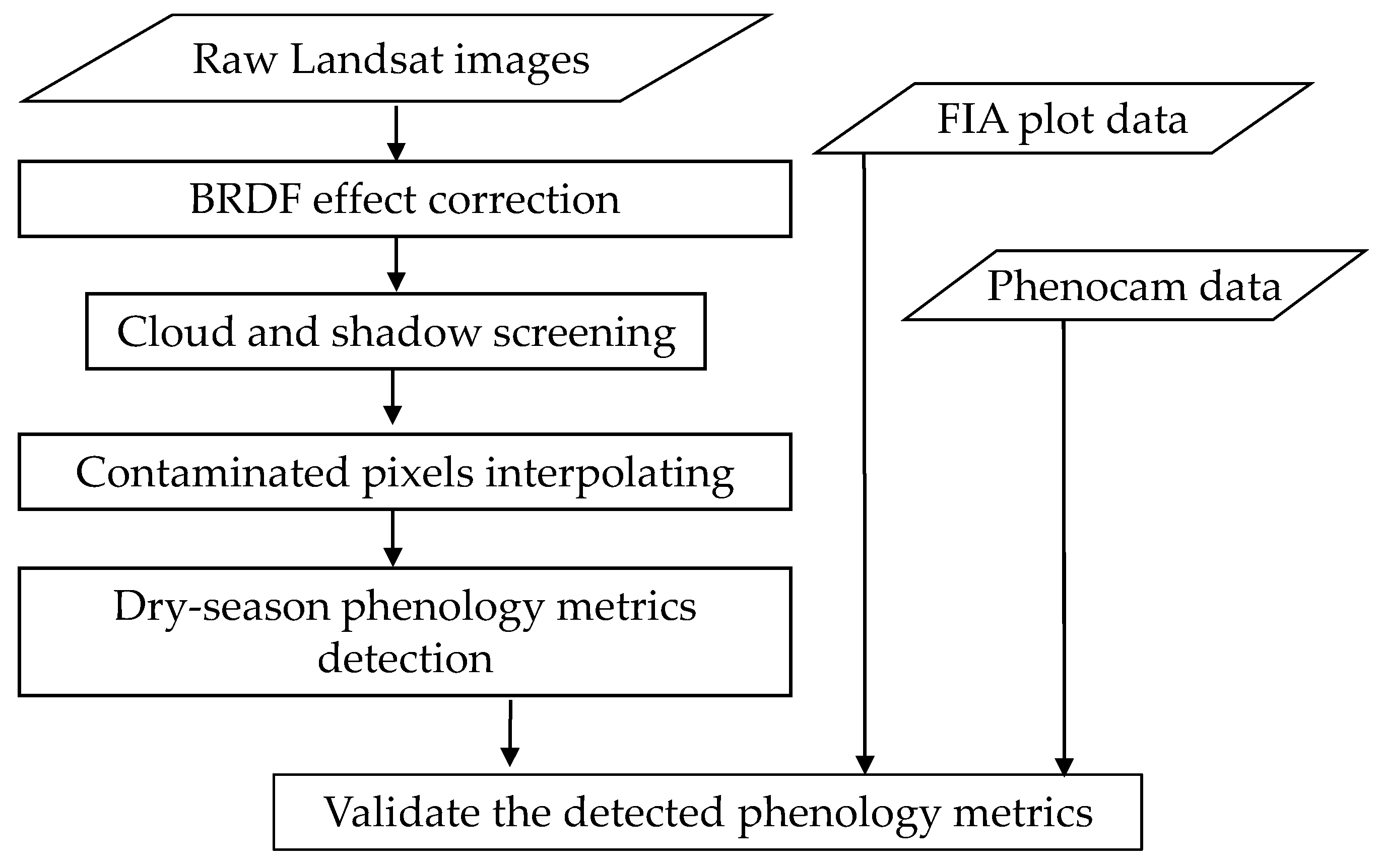
The proposed method includes two main steps: generating a cloud-free seasonal Landsat time series and extracting the dry-season phenology metrics (Figure 2). The first step has three processes, including correcting the effect of solar and observational angles on ground reflectance, screening clouds and cloud shadows in the Landsat time series, and interpolating the values of data gaps. Data gaps included pixels covered by clouds and shadows and missing pixels due to failure of the Scan Line Corrector on Landsat-7 (SLC-off gaps). The second step first defined a comprehensive set of metrics that reflects critical vegetation behaviors and then adopted a threshold-based method to extract these metrics. The details are described in the following subsections.

Figure 2.
The flowchart of this study.
3.1. Generating a Cloud-Free Seasonal Landsat Time Series
3.1.1. BRDF Effect Correction
It is well known that the vegetation reflectance varies with the solar and observational angles, which can be characterized by a BRDF. Previous studies have found that BRDF correction can improve the accuracy of vegetation phenology detection from satellite time series [42,43,44]. The solar angle of Landsat imagery over Puerto Rico varies with day of year, specifically, the sun zenith angle changes from 50° in spring to 25° in summer, while the sun azimuth angle changes from 140° in spring to 75° in summer. In addition, Landsat sensors acquire images at view angles ±7.5° from nadir that cause small directional effects in surface reflectance [41]. Therefore, the observations in Landsat time series have significant BRDF effect that should be adjusted. The BRDF correction adjusts images in Landsat time series to consistent solar and view angles. In this study, we adopted the Landsat BRDF adjustment method that uses MODIS BRDF parameters [41].
In general, the BRDF correction is achieved using the Ross-Li BRDF model, as in Equation (1). The viewing angle is set to nadir, while the solar zenith angle is corrected to a uniform angle (30° in Puerto Rico).
where , , and are the solar zenith angle, viewing zenith angle, and relative azimuth angle, respectively. and are the volume scattering kernel and the geometric optical kernel, respectively. is isotropic reflectance constant, and and refer to the weight coefficients of volume scattering kernel and geometric optical kernel. The parameters , , and are related to the spectral bands and land cover types, which can be obtained from the MODIS BRDF parameter product (e.g., MCD43A2) and are summarized in a previous work (see Table 5 of the paper [41]).
The volume scattering kernel () is derived from the radiative transfer model proposed by Ross in 1981 [45].
The geometric optical kernel () can be obtained from the geometric optical model proposed by Li and Strahler in 1992 [46], as in Equations (4)–(9):
X is limited to the range (−1, 1)
The of original solar and viewing angles and the of adjusted angles in each pixel can be calculated by the Ross-Li BRDF model. Afterwards, the ratio of and is further used to correct original reflectance () to BRDF-corrected reflectance (), as in Equation (10).
3.1.2. Screening Clouds and Cloud Shadows
Optical satellite images over tropical regions are often contaminated by clouds and cloud shadows [47]. This cloud contamination reduces vegetation index (VI) values, which adds significant noise to VI time series being used for phenology detection. Therefore, it is necessary to mark these contaminated pixels in the Landsat images. The Landsat level-2 products have a cloud quality assessment (QA) band that is generated by a single-image based cloud detection method [37]. It has considerable commission and omission errors in tropical areas, especially omission errors for thin clouds [38]. To solve this problem, this study employed a time-series based cloud detection method—automatic time series analysis (ATSA) [36]—to screen clouds and shadows in the Landsat images.
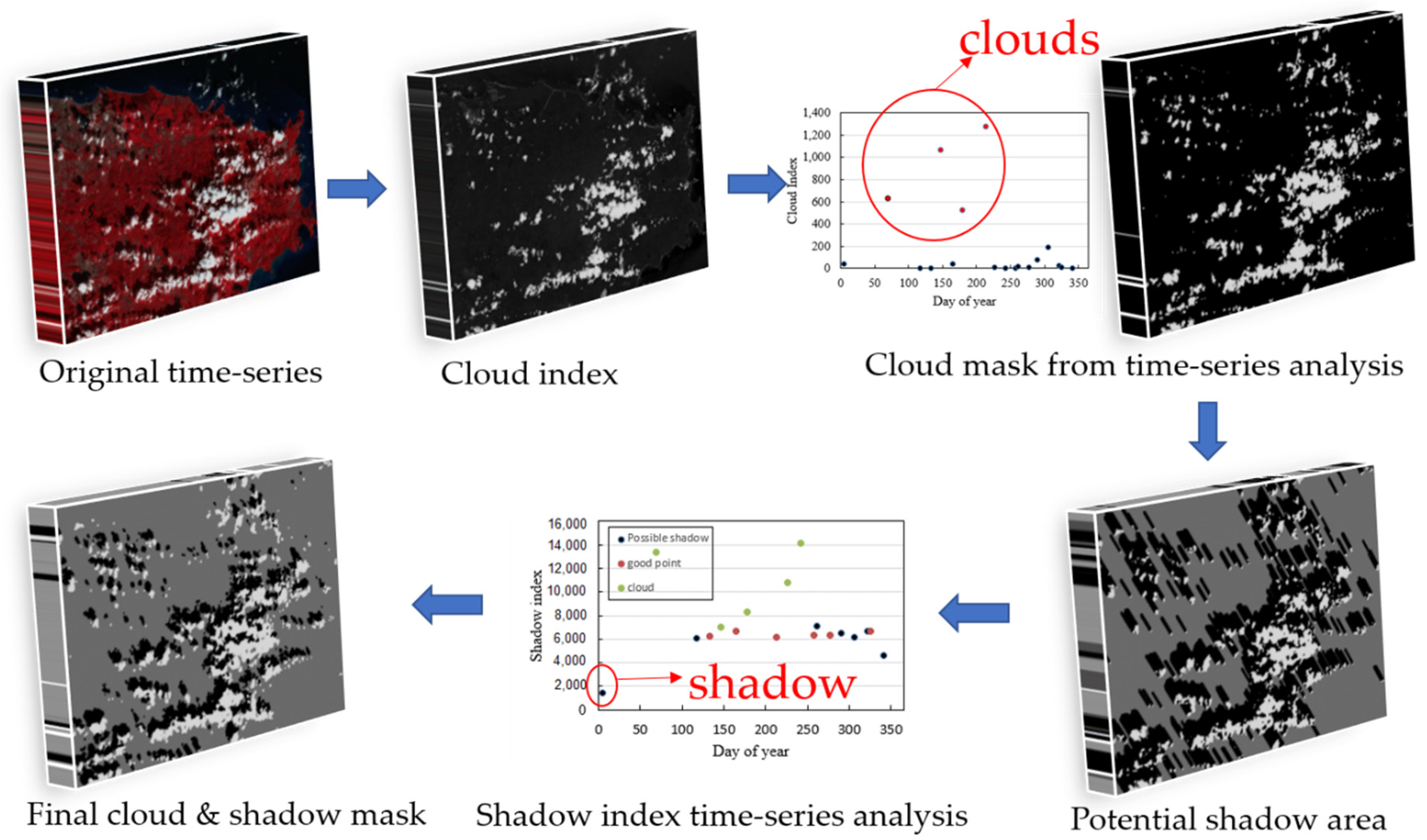
The principle and process of ATSA are shown in Figure 3. ATSA uses the following characteristics of clouds and shadows: (1) clouds can be distinguished from other land covers in the blue-red spectral space, (2) shadows are darker than surrounding pixels outside of shadows, (3) shadows are paired with clouds, and (4) clouds and shadows are significantly different from clear observations in the time series. According to above characteristics, ATSA has five steps to develop cloud and shadow masks for all images in a time series (Figure 3). First, cloud and shadow indices were calculated to highlight cloud and cloud shadow information. The cloud index for land is an automatically derived haze optimized transform () that indexes deviations from the linear relationship between the red and blue bands for clear-sky pixels (Equation (1) in [36]). The shadow index (SI) for land is the sum of the near infrared (band 4) and first shortwave infrared bands (band 5) (Equation (4) in [36]). Second, an initial cloud mask was produced by an unsupervised classifier k-means that automatically partitions HOT values of all pixels into cloud and non-cloud clusters. Third, the initial cloud mask was refined by analyzing the HOT time series, i.e., the observation with a HOT value higher than the adaptive threshold was designated as clouds according to Equation (11).
where { } is the standard deviation of the index through the time series, is the index value of the ith pixel at time , and is the set of cloudy points from the initial masks for the ith pixel. A is a standard deviation multiplier that defines the upper boundary. A can be assigned a recommended value from 1 to 2. Fourth, the potential shadow mask was estimated using geometric relationships with the locations of clouds. Last, the potential shadow mask was refined by analyzing the time series of the shadow index, i.e., observations with a shadow index lower than the adaptive threshold were designated as shadows according to Equation (12).
where is a standard deviation multiplier that serves as a parameter to tune the threshold, mean is the mean of pixel i for the time series, and is the standard deviation of the for the clear observations of pixel . The recommended value of B is from 1 to 3, and a larger value will select darker shadows. and are the two most important parameters that balance the commission and omission errors of cloud and shadow detection. In this study, to reduce the omission errors, and are set as 0.5 and 1, respectively.
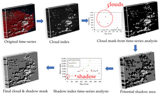
Figure 3.
Principle and process of ATSA for screening clouds and shadows in Landsat time series (the reflectance value of pixels was rescaled to 0–10,000 for computing cloud and shadow indices).
3.1.3. Interpolating Contaminated Pixels in the Time Series
The time series composed of raw Landsat 7 or 8 images includes many pixels covered by unscanned gaps (with Landsat 7), clouds, and shadows since images with up to 50% cloud cover were selected for the time series. With daily satellite images, such as MODIS and AVHRR, contaminated pixels are often removed with maximum value compositing (MVC) and time series smoothing filters [48]. Both MVC and smoothing filters rely on the clear observations for each pixel in the time series. However, the observations from fine resolution multispectral imagery like Landsat are much sparser than MODIS and AVHRR, and they are particularly sparse in many tropical regions before the launch of Landsat 8 in the year 2013 and Sentinel-2 in 2015. Consequently, the MVC and smoothing filters cannot be applied to older Landsat time series in many regions. As an alternative, this study employed the nearest similar pixel interpolator (NSPI) method [39] to interpolate contaminated pixels, including the pixels covered by clouds and cloud shadows and pixels within the un-scanned gaps in Landsat-7 ETM+ images. Unlike the MVC and smoothing filters, NSPI takes advantage of both the temporal and spatial information in clear pixels. It can produce good results even where clear observations are temporally sparse. Although more complicated interpolation methods have been developed, such as deep learning ones [40,49], NSPI was used in this study because: (1) vegetation phenology is a gradual land surface change, and NSPI has been proven effective for interpolating pixels with such gradual change [50]; and (2) its high efficiency makes it feasible to process a large amount of Landsat images.
NSPI was first proposed to interpolate the missing pixels in SLC-off ETM+ images [51]. It uses the following principles: (1) nearby pixels from the same land cover share high spectral similarity, and those pixels are referred to as similar pixels; (2) similar pixels have a consistent temporal change pattern in the time series; and (3) similar pixels have spatially autocorrelated spectral reflectance, and the autocorrelation is stable in the time series. Therefore, NSPI uses both spatial autocorrelation information and temporal change information to estimate the pixel value, respectively, as Equations (13) and (14).
where and are the spatial prediction and temporal prediction of pixel (i.e., the target pixel) at time for band b, and are the band b value of the similar pixel in the ancillary image acquired at and the target image , respectively, and is the weight of the similar pixel that is determined by the spatial and spectral distances between the target pixel and similar pixels. Then, a weighted average of these two predictions yields the final prediction of the target pixel:
where the weights ( and ) are determined by the extent of spatial continuity and the extent of temporal continuity between the ancillary image and the target image estimated from similar pixels. The NSPI method was further modified (i.e., MNSPI) for restoring the spectral values of cloudy pixels by considering the difference between narrow wedge-shaped SLC-off gaps and clouds [52]. It should be noted that both NSPI and MNSPI were implemented to remove contaminated or missing pixels in individual Landsat images. For reconstructing time series, NSPI and MNSPI have been integrated into an iterative framework that automatically interpolates contaminated or missing pixels in all images in a time series [39]. Here, we use the NSPI program coded in interactive data language (code is available at https://xiaolinzhu.weebly.com/, accessed on 1 August 2021) to obtain a high-quality time series from the raw Landsat time series.
3.2. Extracting the Phenological Metrics
Existing studies have widely used satellite VI time series to extract several critical phenology metrics during the growing season, such as green-up. Inflexion-based and threshold-based methods are two types of widely used approaches to extract vegetation phenology from VI time series [53]. They were adopted by NASA and the United States Geological Survey (USGS) to produce phenology products, respectively. The inflexion-based method identifies the inflection point of VI time series to define phenology metrics, whereas the threshold-based method determines phenology dates with a predefined percentage of change in VI [54]. For example, in some studies the green-up date is the day that VI values reach 20 percent of their maximum amplitude [55,56]. Since the threshold-based method is simple and generally consistent with the inflexion-based method [54], we extracted dry-season phenology metrics with threshold-based methods.
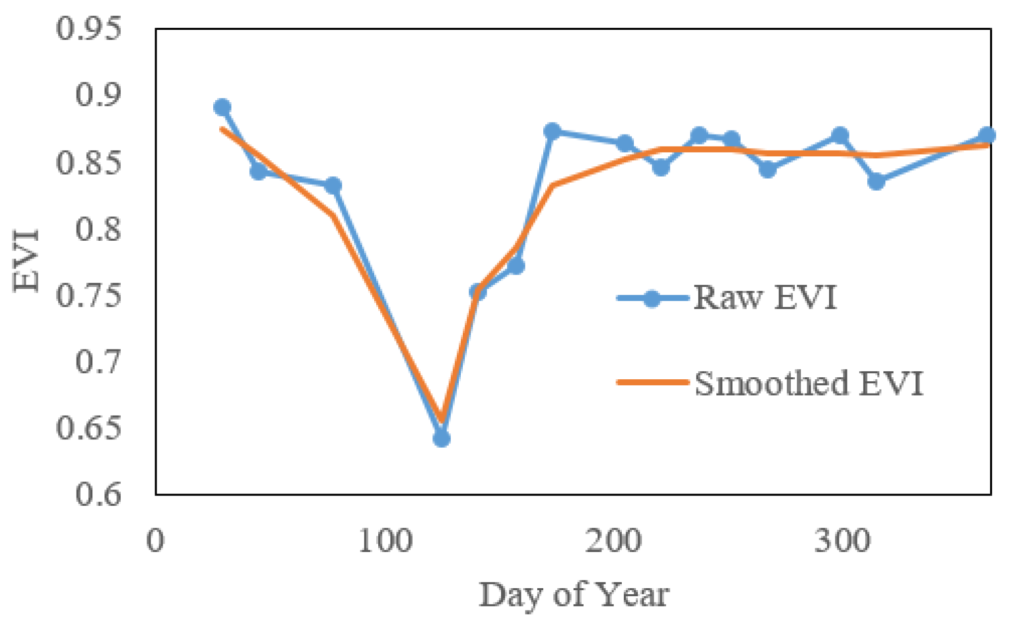
We extract phenology metrics with two steps. The first step is to interpolate and smooth the reconstructed cloud-free VI time series to create a daily VI time series. After applying the technologies in Section 3.1 to obtain a cloud-free Landsat time series, we calculate VI values from the Landsat images. Existing studies use the normalized difference vegetation index (NDVI) and enhanced vegetation index (EVI) to detect phenology. Here, we focused on EVI because background noise affects it less, and it is more sensitive in areas with dense vegetation. Our initial exploration found that in our study area, EVI phenology agrees better with ground observations than does NDVI (R2: 0.69 vs. 0.48). However, the EVI time series derived from the reconstructed cloud-free images have unequal time intervals and still contain minor noise (see an example in Figure 4). Therefore, the raw EVI time series were smoothed with a Savitzky–Golay-filter-based method [57] and interpolated to daily time intervals using the Spline method [58] (Figure 4). Additionally, considering that the reconstructed Landsat time series is not reliable if clear observations in the original time series are too limited, the pixels with fewer than 10 clear observations were excluded from our study area for phenology extraction. These excluded pixels occur mainly in the east part of main island of Puerto Rico (Figure 5).
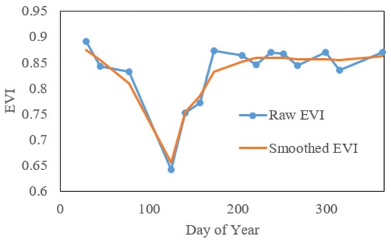
Figure 4.
An example of raw and smoothed EVI time series in Puerto Rico.

Figure 5.
Number of cloud-free Landsat 7 ETM+ observations in the western part of the main island (left) and Mona (right) from the years 2005–2009. Pixels with fewer than 10 cloud-free observations are in wetter forest areas in the east, and at the highest elevations (600 to 1300 m).
Then, the one-year time series is duplicated to a three-year time series, considering that the dry-season cloud be across two adjacent years. This strategy has been used by TIMESAT, a widely used software for detecting growing-season phenology metrics [55]. The lowest EVI value is searched from the smoothed time series, and the major dry season is identified by searching the maximum EVI values before and after the lowest EVI value. Subsequently, 15 metrics can be extracted, given the major dry season, using the definitions in Table 2 and Figure 6. These 15 metrics compose a comprehensive set of phenology variables that include popular ones (e.g., the greenup date, browndown date, and peak date) in existing studies, and ones that describe vegetation processes such as the greenup rate and integral over the dry season, which may have links with climate variables, leaf habit, or vegetation biophysical factors. It should be noted that all phenology detection methods may output extreme values for some pixels and other unexpected noise. Therefore, existing studies often constrain the vegetation growing period to obtain reasonable phenology metrics. For example, a study in north China assumes that the greenup date should occur between March and July [59]. To reduce noise in phenology metrics in our study, all vegetation pixels in the study area were clustered according to the similarity of their EVI profiles with the k-means method. Then, the average date of lowest EVI in each cluster (cluster-average lowest date) was used as a reference to constrain the search for the lowest EVI at the pixel level. The time window searched for the lowest EVI of a pixel is within the 60 days of the cluster-average lowest date.

Table 2.
15 dry-season phenological metrics extracted from the EVI time series.

Figure 6.
Definition of dry-season phenology metrics in the enhanced vegetation index (EVI) time series: (a) a–f are maximum EVI, minimum EVI, amplitude, browndown date, greenup date, and dry season length; (b) the light gray shaded area is the small integral over growing season, the orange shaded area is integral over dry season, and the total of light gray and light green shaded area is large integral over growing season; and (c) the gray and green shaded areas are small and large integral of the whole year, respectively.
3.3. Validation
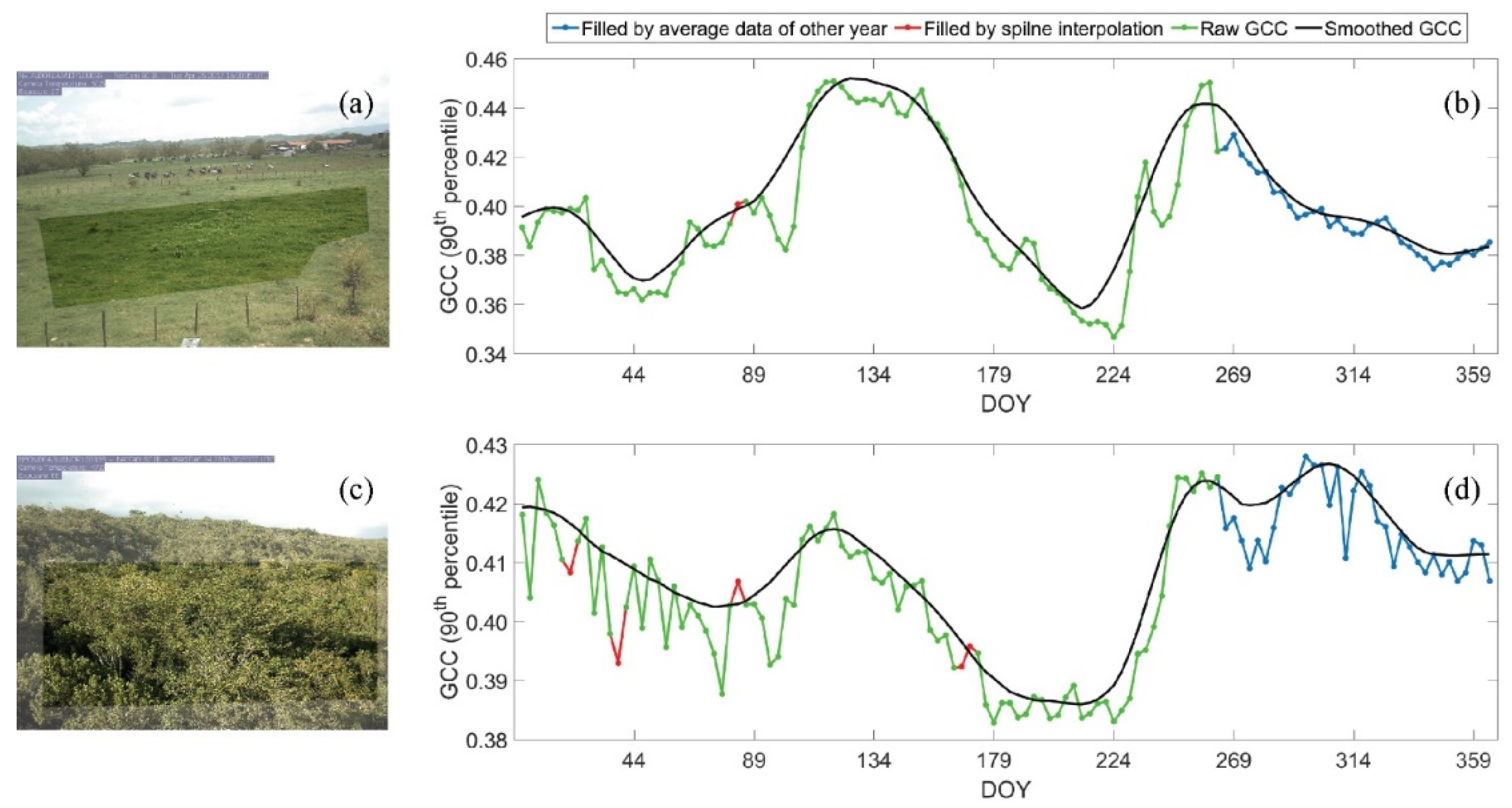
For the validation of the phenology metrics, we adopted both direct and indirect ways to assess the accuracy. Where at least 50% of the observations in the time series were clear, which was in tropical dry forest zones, we assessed the accuracy directly. We compared the phenology dates (e.g., dates of greenup, lowest, and browndown) derived from Landsat time series with that derived from two PhenoCam sites (locations are shown in Figure 1). Following a previous study [60], we used the 90th percentile of values of the region of interest (ROI) within a 3-day moving window, which can depict the data trajectory well and has fewer effects from outliers, to compose the raw green chromatic coordinate (GCC) time series in each PhenoCam site (Figure 7). The missing data in the GCC time series within 7 days were interpolated by spline interpolation, while the missing data beyond 7 days were filled with average data from adjacent years (Figure 7). We further smoothed the GCC time series by applying an iterative Savitzky–Golay (SG) filter [57], represented by the black lines shown in Figure 7b,d. Then, the phenology metrics were extracted from the smoothed GCC curve using the definitions in Table 2. Last, the phenology metrics of Landsat pixels within the orientation of the PhenoCam and with same vegetation type with the ROI of the PhenoCam were selected for the comparison.
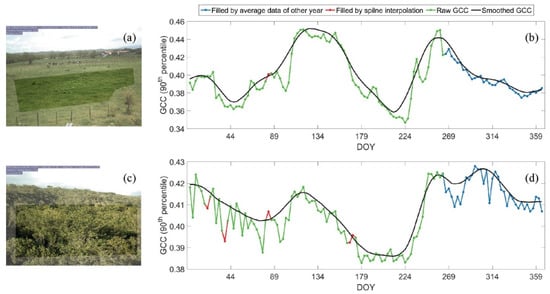
Figure 7.
The region of interest (ROI) of photos in PhenoCam site A (a) and PhenoCam site B (c) and their derived GCC time series in 2017 (b,d) in the tropical dry forest zone of Puerto Rico. DOY: day of year.
However, the number of PhenoCam sites in our study area was too limited to obtain a reliable assessment. Therefore, we also employed an indirect way to validate the phenology results through linking the phenology metrics with the vegetation biophysical variables since studies have found that phenology of tropical vegetation was correlated to vegetation structure [61,62]. Specifically, the indirect validation was implemented on Mona Island using ground observations of and leaf area index (LAI) [63] and aboveground live biomass (AGLB), which were derived from the 26 FIA plots collected in 2008 [64]. These 26 plots are spaced every 2 km2 across the island. Plots have four circular 0.016 ha subplots, where trees with a diameter at breast height (dbh) of ≥12.7 cm are surveyed. Trees 2.5–12.6 cm dbh (small trees) are surveyed on 2.07-m radius circular microplots within each subplot. The four subplots include a center subplot and three surrounding subplots with centers located 36.6 m from the plot center at azimuths of 360, 120, and 240 degrees respectively. Consequently, the plot size is roughly equivalent to a 3 × 3-window of Landsat pixel (size of 30 m × 30 m), so the phenology metrics of each plot were collected by averaging the phenology metrics values of a 3 × 3 window of pixels centered on the plot. Data for leaf area index (LAI) were collected on two subplots within each of 22 of the plots. Stepwise regression was used to build statistical models between phenology metrics (i.e., independent variables) and AGLB and LAI (i.e., dependent variables), respectively. Since sample numbers are limited for both AGLB and LAI, we assessed regression model performance with the leave-one-out method.
4. Results
4.1. Accuracy of Landsat Time Series Reconstruction
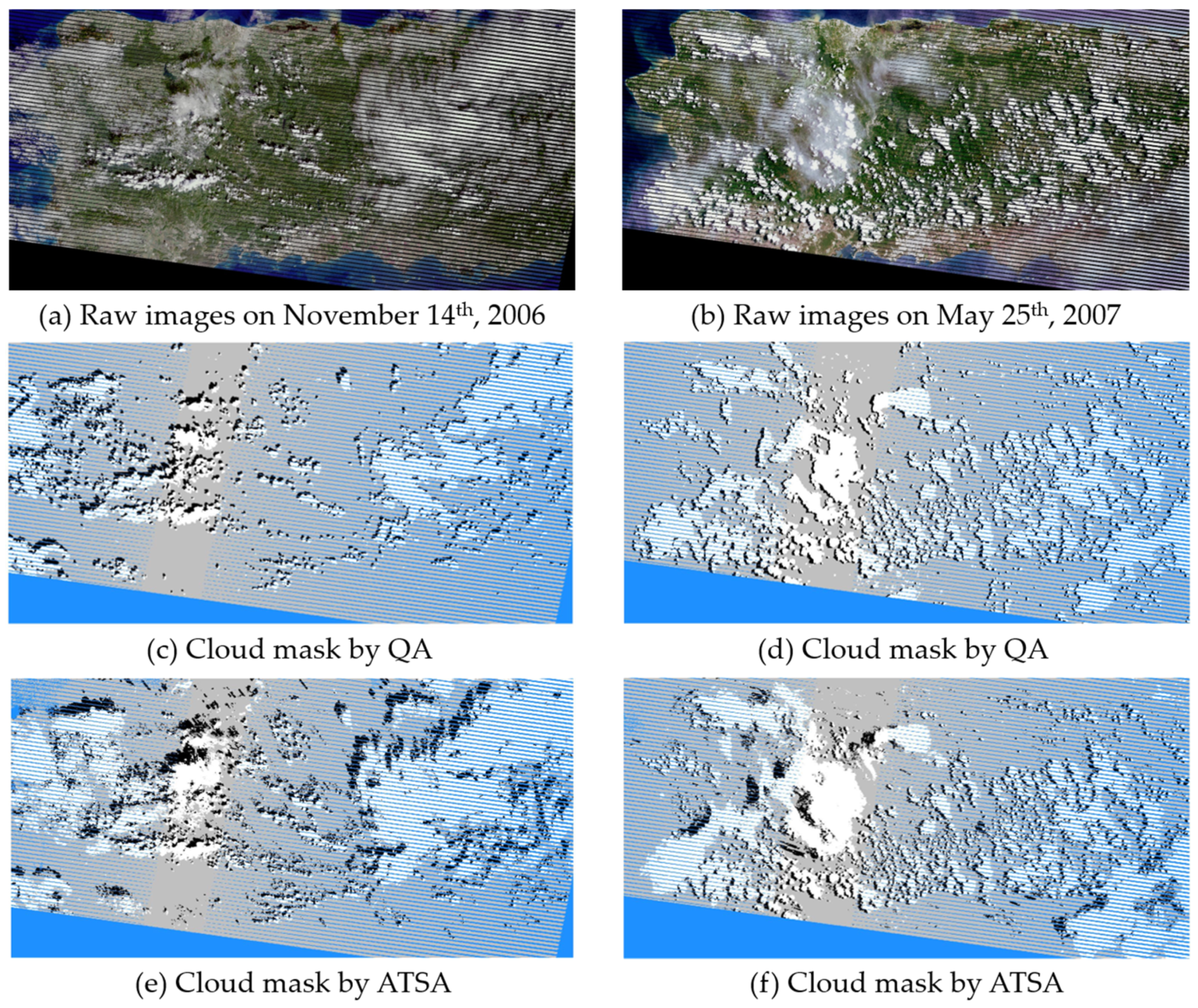
Comparing cloud and shadow masks from ATSA with those from the Landsat cloud QA band (Figure 8), two representative raw Landsat images over mainland Puerto Rico show that ATSA successfully identified nearly all clouds and shadows, but the Landsat QA band omits a considerable number of thin clouds. To quantitatively compare accuracies of the Landsat QA band with ATSA, the clouds and shadows in these two images were manually digitized as reference data. The accuracy indices derived from an error matrix show that ATSA is more accurate than the Landsat QA band for cloud and shadow detection (Table 3). Specifically, the producer’s accuracy of ATSA is higher than 0.9 for both clouds and cloud shadows, indicating very small omission errors, but the QA band has large omission errors in both clouds and cloud shadows. In this study, it is important to control omission errors since they will affect the subsequent cloud removal step. Therefore, we used relatively small values of both parameters A and B in ATSA to detect suspected clouds and cloud shadows as much as possible, accepting some commission errors since they do not affect the following cloud removal step. To further reduce the effect of omission errors on the cloud removal step, cloud and shadow masks from ATSA were buffered by the width of one pixel before applying the NSPI step.
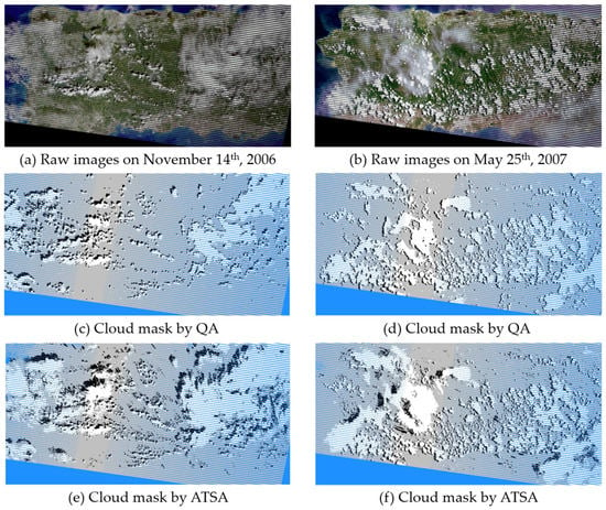
Figure 8.
Two true-color raw Landsat-7 images on 14 November 2006 (a) and 25 May 2007 (b) over the main island of Puerto Rico, and the corresponding cloud and shadow masks extracted by Landsat cloud QA band (c,d) and ATSA method (e,f). The write, black, and blue in the masks are clouds, shadows, and gaps.

Table 3.
Accuracy assessment of cloud and cloud shadow masks of two images in Figure 8: overall accuracy (oa), user’s accuracy (ua), and producer’s accuracy (pa).
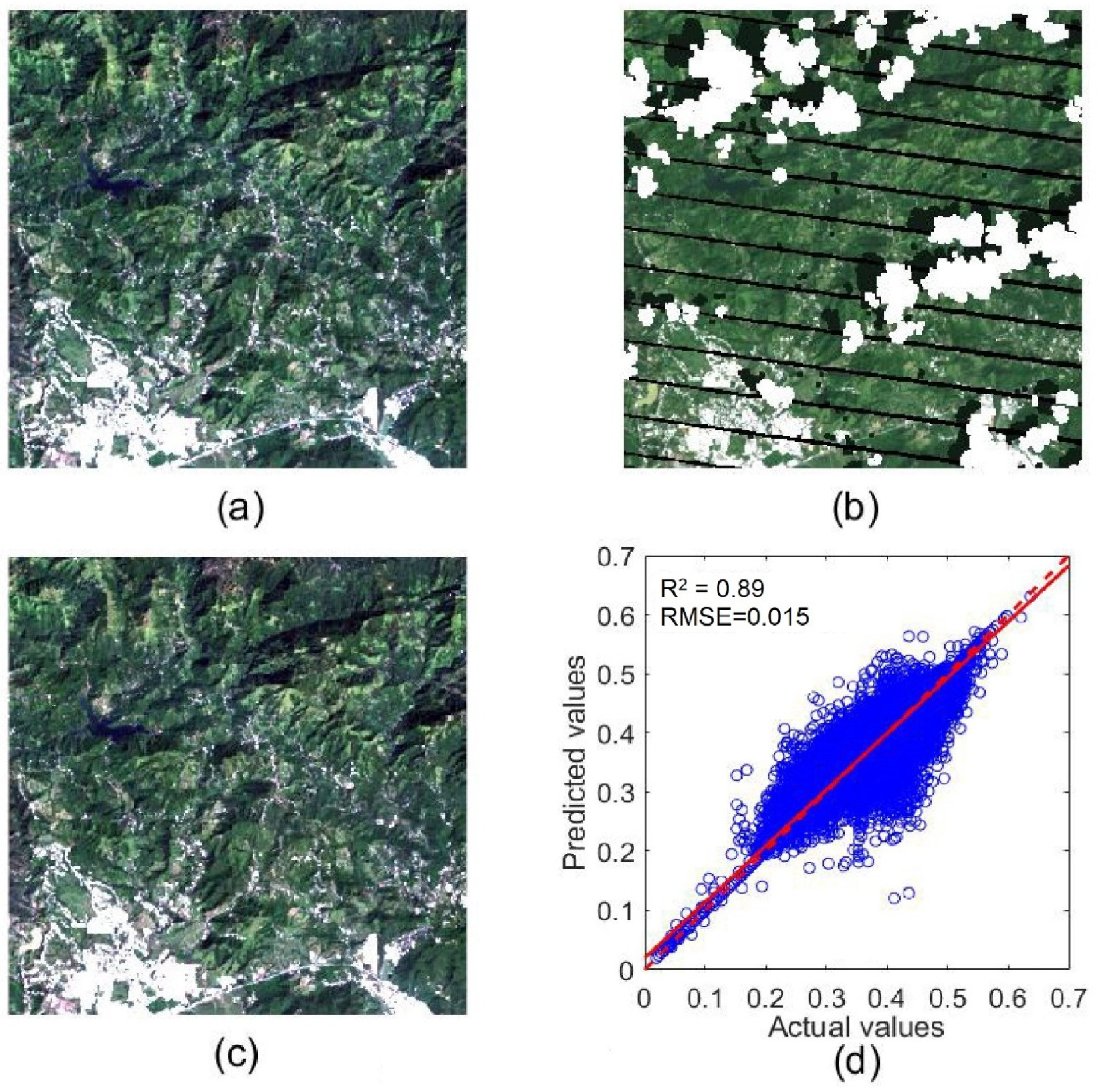
To quantitatively assess the accuracy of contaminated pixel interpolation, we selected a cloud-free subset from our collected Landsat time series as a reference image (Figure 9a, its location is marked by a box in Figure 1). Then, to simulate a cloudy image, we added to this reference image gaps, clouds, and shadows extracted from a cloudy image (Figure 9b). For this simulated cloudy image, its real pixel values were used to assess the accuracy of cloud removal and gap filling by NSPI (Figure 9c). We can see that nearly all gaps, clouds, and shadows were successfully removed by the NSPI method. The repaired image has high-quality visuals. The repaired pixels have high consistency with surrounding clear pixels, and the places with clouds and shadows are nearly invisible in the reconstructed image, suggesting that the reconstructed image has high accuracy. The scatter plot between actual and predicted values for the NIR band (Figure 9d) also demonstrates the high accuracy of the NSPI interpolation results. The NIR band changes more with vegetation growth and so is more challenging to interpolate than other bands. The RMSE value is 0.015 and R2 value is 0.887 for the NIR band in this simulation experiment, suggesting that the reconstructed images can reliably capture the vegetation dynamics.
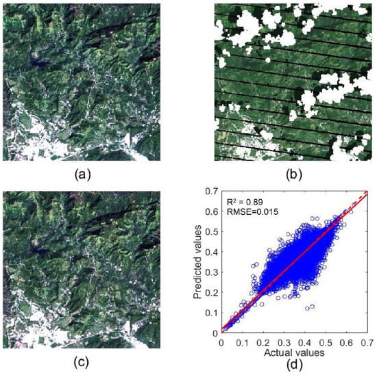
Figure 9.
A true-color clear sub-image on 18 October 2008 (a); the corresponding simulated cloudy image (b); gap, cloud, and shadow removed by NSPI (c); and the scatter plot between the actual values and predicated values of NIR band (d).
4.2. Maps and Reasonability of Detected Phenology Metrics
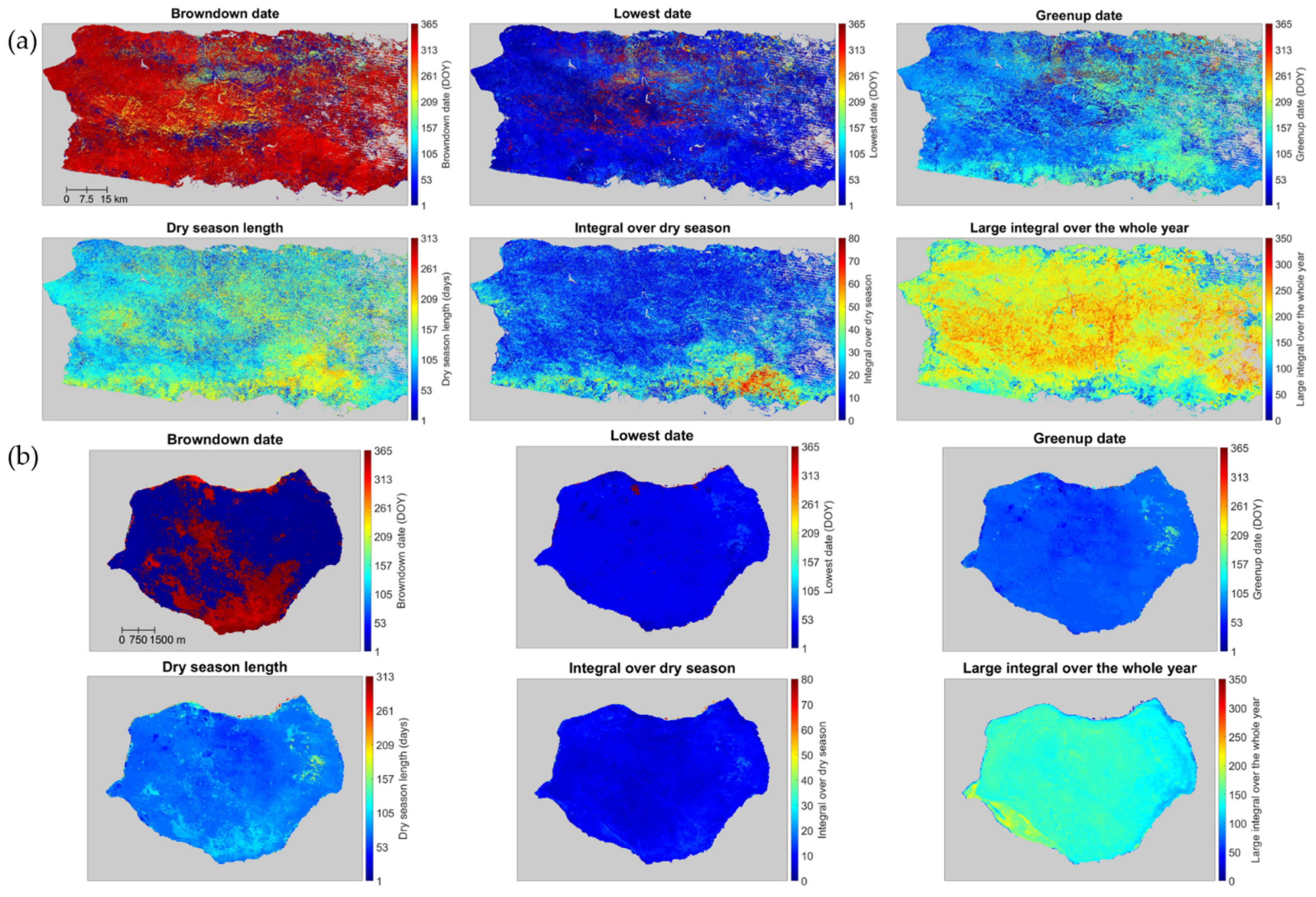
The spatial pattern of several representative phenology metrics derived from reconstructed Landsat images, for both the main island and Mona, has high spatial heterogeneity (Figure 10). The integral over the dry season shows that the southern zone of the main island is more affected by the dry season. The forests in the south are drier and have larger relative basal areas of deciduous tree species. Their dry season is longer in Figure 10a. The phenology metrics also show that the majority of the main island enters the dry season (i.e., browndown date) at the end of a year and that the end of the dry season (i.e., greenup date) is around May. The large integral over the whole year shows the locations where the vegetation is green throughout the year, with orange to red tones, and a dry season length of less than 90 days (blue tones). Evergreen tree species dominate the majority of these areas, and the aboveground biomass density is larger [19]. These patterns are consistent with the climate in Puerto Rico. The wettest month on the island is August, with 18 cm of rain. Puerto Rico’s rainy season lasts from April to November, and the driest season is December to March.
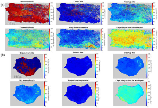
Figure 10.
Representative phenology metrics derived from the reconstructed Landsat time series in main island (a) and Mona (b): browndown date, lowest date, greenup date, dry season length, integral over dry season, and large integral over the whole year. Gray pixels are background, water, and pixels with clear observations fewer than 10 during 2005–2009.
Across the middle of the island, several areas with blue to green colors for the large integral correspond to areas with lower biomass density. Although these areas are at higher elevation and have more rainfall, the combination of climate and geology (geoclimate) makes growing conditions more challenging, as reflected by the larger relative basal area of tree species with stiff evergreen leaves since these areas include cloud forests and forests growing on fast-draining serpentine or karst substrates [19].
4.3. Validation Results of Detected Phenology Metrics
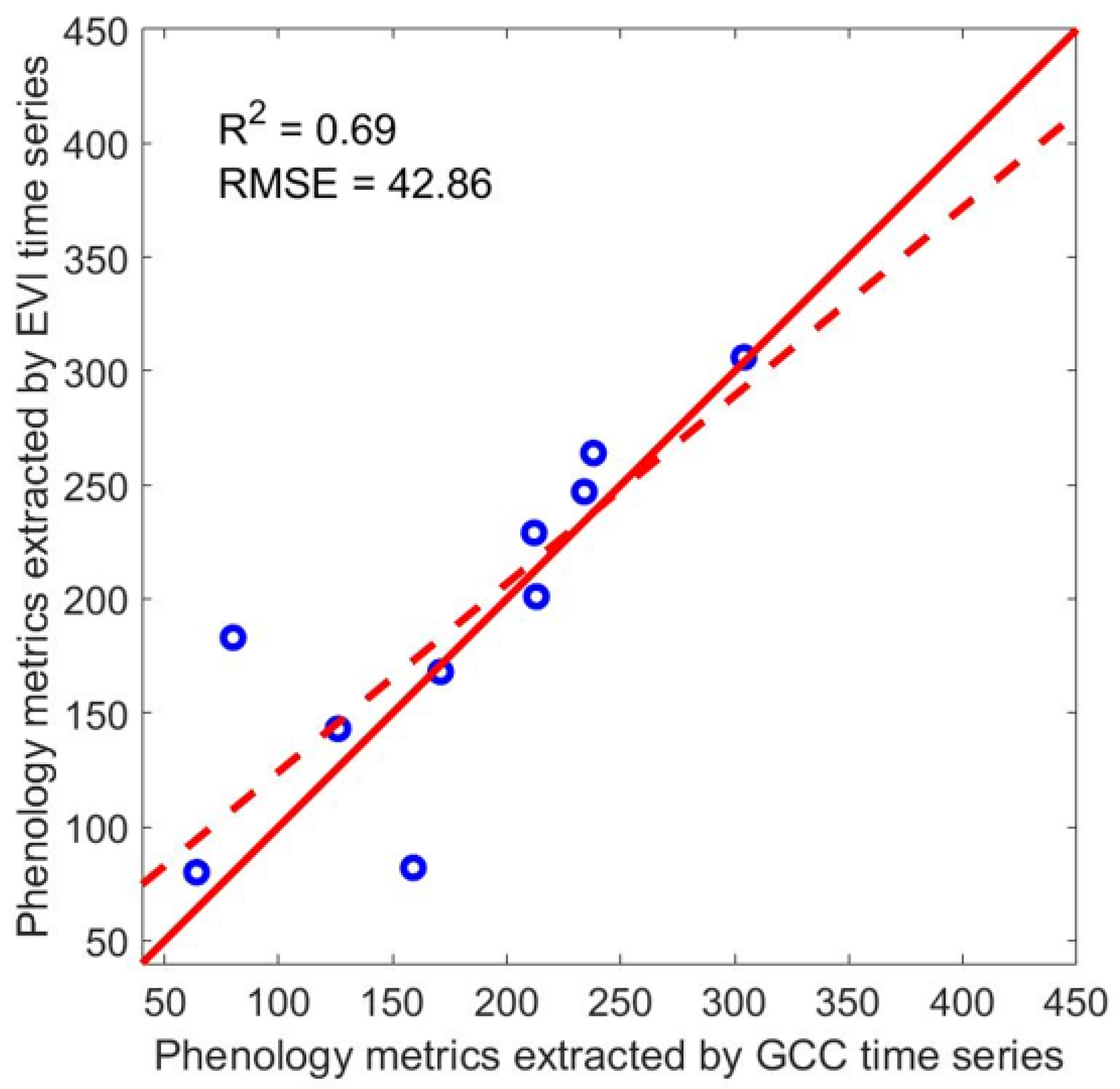
Table 4 shows the comparison between phenology metrics extracted from the reconstructed Landsat EVI time series and the PhenoCam GCC time series for two PhenoCam sites and five phenology metrics: peak date, lowest date, greenup date, browndown date, and dry season length, and these values were plotted in Figure 11. It shows that the phenological results from reconstructed Landsat EVI time series generally agree well with those from the ground-based observations (R2 = 0.69). We inspected the EVI time series of PhenoCam B and found that the time series was over-smoothed, so it does not have the small wave in GCC from DOY 89 to DOY 179 (Figure 7d). This caused the browndown date detected from Landsat EVI to be much earlier than that from PhenoCam GCC.

Table 4.
Summary statistics of phenology metrics extracted by Landsat EVI time series and PhenoCam GCC time series in two PhenoCam sites.
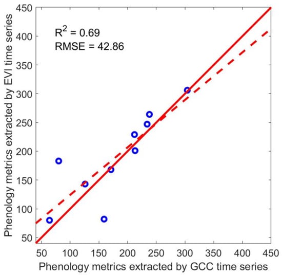
Figure 11.
Comparison between phenology metrics derived from Landsat EVI time series and that from the two PhenoCam sites in the tropical dry forest zones of Puerto Rico, including 5 phenology metrics: peak date, lowest date, greenup date, browndown date, and dry season length.
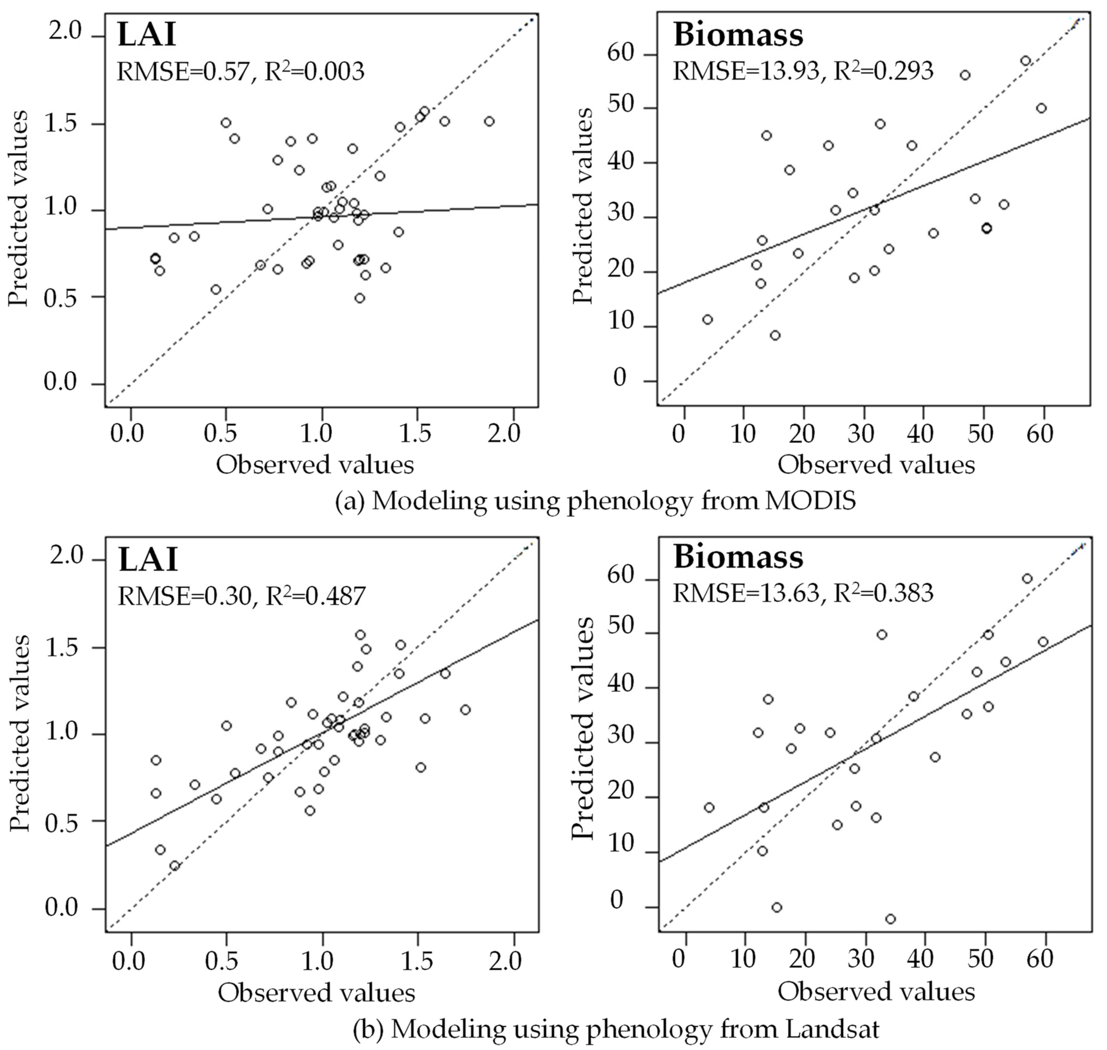
In the indirect validation, using phenology metrics from reconstructed Landsat time series improves models of LAI and aboveground live biomass, compared with phenology derived from MODIS time series (Figure 12). For LAI modeling, the RMSE value of using Landsat phenology metrics is much lower than using MODIS (0.30 vs. 0.57), and R2 value is much higher than MODIS (0.487 vs. 0.003). For aboveground live biomass modeling, the RMSE value is similar between Landsat and MODIS, but the R2 of Landsat is higher than MODIS (0.383 vs. 0.293). It is well known that MODIS has high frequency but coarse spatial resolution, but it cannot accurately model the biophysical variables of FIA plots in the tropical dry forest of Mona Island because its pixel size is much larger than the FIA plot. In contrast, Landsat pixels have a size comparable with the FIA plot, so that the phenology metrics can better represent the biophysical variables estimated on the plots. This result suggests that for tropical dry forest, the Landsat based phenology metrics are reliable.

Figure 12.
Leave-one-out validation results from modeling LAI and biomass using phenology metrics derived from a MODIS time series (a) and a reconstructed Landsat time series (b) in the tropical dry forest of Mona Island, Puerto Rico.
5. Discussion
5.1. Implications for Tropical Forest Monitoring
In this study, we evaluate an approach for characterizing vegetation seasonality in tropical dry forest landscapes, including metrics focused on both the dry season and growing season, using seasonal patterns of vegetation greenness indices (land surface phenology) with Landsat multispectral satellite imagery. The results and proposed approach have three implications for future tropical forest studies: (1) the finer spatial scale of phenology metrics extracted from Landsat can link more strongly to tropical dry forest LAI and biomass, two important biophysical attributes, as estimated in ground inventory studies; (2) by explaining more variability in these attributes, the method may better support studies of climate and vegetation interactions at fine scales in tropical dry forest landscapes; and (3) in wetter tropical forest landscapes, aggregating Landsat images from multiple years may map forest phenology reliably.
Regarding spatial scale, most forest ground plots are 0.1 to 1 ha in size, the size of one or more Landsat pixels, which is much smaller than the 6 to 25-ha size of high frequency optical satellite image bands like those in MODIS imagery (though some plots are up to 50 ha in size). Regarding remotely sensed phenology at Landsat scale, multi-season imagery and land surface phenology with high spatial resolution permit detailed land cover and agriculture mapping in drier tropical areas [35,65,66]. Imagery with 3- to 30-m pixels is now widely available and has advantages for evaluating tropical forest response to climate change in past studies as well. Land surface phenology from Landsat or Sentinel 2 (10–60 m), as compared with single-date imagery, improves mapping and modeling of productivity and carbon stocks of tropical dry forest and savanna landscapes [67,68,69]. Dry season intensity is a defining feature of tropical dry forests and savannas, influencing forest structure, productivity, carbon storage, functional traits, fire ecology, ecohydrology, and tree species composition and diversity [20,70,71,72]. Drought and dry seasons typically reduce canopy greenness in drier, more seasonal forests, where water availability tends to limit productivity [73,74].
5.2. Limitations and Future Studies
Although we applied state-of-the-art technologies to reconstruct cloud-free Landsat images, challenges remain. First, the thin clouds and haze in older Landsat images without the Cirrus band are difficult to detect. These include Landsat 4 and 5 TM, Landsat 7 ETM+, and the earlier Landsat MSS images [39]. Omitting these thin clouds and hazy areas in cloud masks will cause significant errors because these pixels are considered to be clear observations that are then used to interpolate other cloud pixels. Cirrus clouds will cause the interpolated pixels to be brighter than the surrounding cloud-free pixels. In the EVI time series, these errors will cause EVI values to be lower than the actual values. If we use a smaller value for parameter A in the ATSA method to better detect thin clouds and haze, significant commission errors will result, i.e., many clear observations will be detected as clouds. That result would reduce the number of clear observations in subsequent steps. Therefore, future studies need to improve the cloud detection method for satellite images without the Cirrus band.
Second, the accuracy of cloud removal by NSPI is affected by cloud size and time interval between clear and cloudy observations [39,52]. Unfortunately, many tropical regions are very cloudy throughout the year. If we only use Landsat images, many years of data may be needed to obtain enough clear observations, due to the long revisit cycle of Landsat of 16 days. Our study treats images from five adjacent years as one year to overcome this problem, but this approach has some problems: (1) the climate is not the exactly same in these adjacent years, so the resulting phenology is more or less a five-year average phenology; (2) vegetation may experience disturbance in these years, such as deforestation, fire, or thinning; and (3) it is still hard to get enough clear observations in five years if the area is extremely cloudy (dark blue areas in Figure 5). Future studies can consider integrating images from multiple satellites, such as daily observations from MODIS, 5-day observations from Sentinel-2 and Landsat, by data fusion technology [75].
Last, due to the limitation of ground observations of the dry-season phenology in Puerto Rico, we only evaluated the phenology results with two PhenoCam sites and tested the effectiveness of the derived phenology metrics for modeling the forest biomass and LAI using ground forest plots. More studies in the future are needed to test the proposed method in different tropical areas and validate the results with more ground-based observations.
6. Conclusions
This study proposed a framework of reconstructing high-quality Landsat time series for monitoring dry-season phenology of tropical forests. The framework employs cutting-edge algorithms, including the BRDF correction algorithm, the automated cloud screening algorithm, and the missing data interpolation algorithm. Fifteen dry-season phenology metrics were defined. These metrics were then extracted from VI time series derived from reconstructed Landsat imagery through a robust phenology-detection method. Validation using field plots and PhenoCam data demonstrated the effectiveness of the proposed framework. Phenology metrics at Landsat scale have some advantages compared to MODIS scale, including: (1) they can better bridge ground forest inventory and satellite observations, and (2) they can better support studies of climate and vegetation interactions at fine scales. This is the first study to test the feasibility of Landsat imagery for monitoring tropical forest phenology. The operational framework introduced in this study for reconstructing high-quality Landsat time series can be adopted by future studies (codes are downloadable at https://xiaolinzhu.weebly.com/, accessed on 1 August 2021). Future studies are needed to investigate the uncertainty of reconstructed Landsat time series in cloudy regions, and the sensitivity of phenology detection accuracy to the number of clear observations in the time series and its effectiveness in other fine-scale satellite imagery and other tropical regions.
Author Contributions
Conceptualization, X.Z. and E.H.H.; Methodology, X.Z., E.H.H. and D.G.; Supervision, E.H.H.; Formal Analysis: X.Z., E.H.H., D.G., J.T., M.C. and S.F.; Data Curation: E.H.H., D.G., J.T., M.C., S.F., H.M.-V., J.K.Z. and E.J.M.-A.; Writing—original draft, X.Z., E.H.H., D.G., J.T., M.C. and S.F. All authors have read and agreed to the published version of the manuscript.
Funding
X.Z. was supported by the National Natural Science Foundation of China (project no. 42022060) and the Hong Kong Polytechnic University (projects no. ZVN6 and ZVVF). This research was supported in part by the U.S. Department of Agriculture, Forest Service (F430-C-16-0017, F430-C-17-0020, F430-19-C-0029, 12445021P0060, 19-CS-11120101-412). The findings and conclusions in this [publication/presentation/blog/report] are those of the author(s) and should not be construed to represent any official USDA or U.S. Government determination or policy.
Institutional Review Board Statement
Not applicable.
Informed Consent Statement
Not applicable.
Data Availability Statement
Not applicable.
Conflicts of Interest
The authors declare no conflict of interests. The founding sponsors had no role in the design of the study; in the collection, analyses, or interpretation of data; in the writing of the manuscript; or in the decision to publish the results.
References
- Bustamante, M.; Helmer, E.H.; Schill, S.; Belnap, J.; Brown, L.K.; Brugnoli, E.; Compton, J.E.; Coupe, R.H.; Hernández-Blanco, M.; Isbell, F.; et al. Chapter 4: Direct and indirect drivers of change in biodiversity and nature’s contributions to people. In Regional Assessment Report on Biodiversity and Ecosystem Services for the Americas; IPBES Secretariat: Bonn, Germany, 2018; pp. 335–509. [Google Scholar]
- Jiang, Y.; Zhou, L.; Tucker, C.J.; Raghavendra, A.; Hua, W.; Liu, Y.Y.; Joiner, J. Widespread increase of boreal summer dry season length over the Congo rainforest. Nat. Clim. Chang. 2019, 9, 617–622. [Google Scholar] [CrossRef]
- Sarvia, F.; De Petris, S.; Borgogno-Mondino, E. Exploring Climate Change Effects on Vegetation Phenology by MOD13Q1 Data: The Piemonte Region Case Study in the Period 2001–2019. Agronomy 2021, 11, 555. [Google Scholar] [CrossRef]
- Asner, G.P.; Alencar, A. Drought impacts on the Amazon forest: The remote sensing perspective. New Phytol. 2010, 187, 569–578. [Google Scholar] [CrossRef] [PubMed]
- Brando, P.M.; Balch, J.K.; Nepstad, D.C.; Morton, D.C.; Putz, F.E.; Coe, M.T.; Silvério, D.; Macedo, M.N.; Davidson, E.A.; Nóbrega, C.C.; et al. Abrupt increases in Amazonian tree mortality due to drought—Fire interactions. Proc. Natl. Acad. Sci. USA 2014, 111, 6347–6352. [Google Scholar] [CrossRef] [Green Version]
- Briant, G.; Gond, V.; Laurance, S.G.W. Habitat fragmentation and the desiccation of forest canopies: A case study from eastern Amazonia. Biol. Conserv. 2010, 143, 2763–2769. [Google Scholar] [CrossRef]
- Baker, J.C.A.; Spracklen, D.V. Climate Benefits of Intact Amazon Forests and the Biophysical Consequences of Disturbance. Front. For. Glob. Chang. 2019, 2, 47. [Google Scholar] [CrossRef] [Green Version]
- Allen, C.D.; Macalady, A.K.; Chenchouni, H.; Bachelet, D.; Mcdowell, N.; Vennetier, M.; Kitzberger, T.; Rigling, A.; Breshears, D.D.; Hogg, E.H.T.; et al. A global overview of drought and heat-induced tree mortality reveals emerging climate change risks for forests. For. Ecol. Manag. 2010, 259, 660–684. [Google Scholar] [CrossRef] [Green Version]
- Zhang, Q.; Shao, M.; Jia, X.; Wei, X. Relationship of Climatic and Forest Factors to Drought- and Heat-Induced Tree Mortality. PLoS ONE 2017, 12, e0169770. [Google Scholar] [CrossRef]
- Mcdowell, N.; Mcdowell, N.; Allen, C.D.; Anderson-teixeira, K.; Brando, P.; Brienen, R.; Chambers, J.; Christoffersen, B.; Davies, S.; Doughty, C.; et al. Drivers and mechanisms of tree mortality in moist tropical forests. New Phytol. 2018, 219, 851–869. [Google Scholar] [CrossRef] [Green Version]
- Powers, J.S.; Vargas, G.; Brodribb, G.T.J.; Schwartz, N.B.; Chris, D.P.; Becknell, J.M.; Aureli, F.; Calderón-morales, R.B.E.; Ana, J.C.C.; María, J.C.; et al. A catastrophic tropical drought kills hydraulically vulnerable tree species. Glob. Chang. Biol. 2020, 26, 3122–3133. [Google Scholar] [CrossRef]
- Mitchard, E.T.A. The tropical forest carbon cycle and climate change. Nature 2018, 559, 2–9. [Google Scholar] [CrossRef]
- Gardner, T.A.; Barlow, J.; Chazdon, R.; Robert, M.; Harvey, C.A. Prospects for tropical forest biodiversity in a human-modified world. Ecol. Lett. 2009, 12, 561–582. [Google Scholar] [CrossRef] [Green Version]
- Barlow, J.; França, F.; Gardner, T.A.; Hicks, C.C.; Lennox, G.D.; Berenguer, E.; Castello, L.; Economo, P.; Ferreira, J.; Guénard, B.; et al. The future of hyperdiverse tropical ecosystems. Nature 2018, 559, 517–526. [Google Scholar] [CrossRef]
- Bi, J.; Knyazikhin, Y.; Choi, S.; Park, T.; Jonathan, B.; Philippe, C.; Fu, R.; Ganguly, S.; Hall, F.; Hilker, T.; et al. Sunlight mediated seasonality in canopy structure and photosynthetic activity of Amazonian rainforests. Environ. Res. Lett. 2015, 10, 64014. [Google Scholar] [CrossRef] [Green Version]
- Cooley, S.S.; Williams, C.A.; Fisher, J.B.; Halverson, G.H.; Perret, J.; Lee, C.M. Assessing regional drought impacts on vegetation and evapotranspiration: A case study in Guanacaste, Costa Rica. Ecol. Appl. 2019, 29, e01834. [Google Scholar] [CrossRef]
- Gonçalves, N.B.; Lopes, A.P.; Dalagnol, R.; Wu, J.; Pinho, D.M.; Nelson, B.W. Both near-surface and satellite remote sensing confirm drought legacy effect on tropical forest leaf phenology after 2015/2016 ENSO drought. Remote Sens. Environ. 2020, 237, 111489. [Google Scholar] [CrossRef]
- Wang, J.; Yang, D.; Detto, M.; Nelson, B.W.; Chen, M.; Guan, K.; Wu, S.; Yan, Z.; Wu, J. Multi-scale integration of satellite remote sensing improves characterization of dry-season green-up in an Amazon tropical evergreen forest. Remote Sens. Environ. 2020, 246, 111865. [Google Scholar] [CrossRef]
- Helmer, E.H.; Ruzycki, T.S.; Wilson, B.T.; Sherrill, K.R.; Lefsky, M.A.; Marcano-Vega, H.; Brandeis, T.J.; Erickson, H.E.; Ruefenacht, B. Tropical Deforestation and Recolonization by Exotic and Native Trees: Spatial Patterns of Tropical Forest Biomass, Functional Groups, and Species Counts and Links to Stand Age, Geoclimate, and Sustainability Goals. Remote Sens. 2018, 10, 1724. [Google Scholar] [CrossRef] [Green Version]
- Roa-Fuentes, L.L.; Templer, P.H.; Campo, J. Effects of precipitation regime and soil nitrogen on leaf traits in seasonally dry tropical forests of the Yucatan Peninsula, Mexico. Oecologia 2015, 179, 585–597. [Google Scholar] [CrossRef] [PubMed]
- Umaña, M.N.; Wright, S.J.; Condit, R.; Pérez, R.; Turner, B.L.; Comita, L.S. Shifts in taxonomic and functional composition of trees along rainfall and phosphorus gradients in central Panama. J. Ecol. 2020, 109, 51–61. [Google Scholar] [CrossRef]
- Ruger, N.; Comita, L.S.; Condit, R.; Purves, D.; Rosenbaum, B.; Visser, M.D.; Wright, S.J.; Wirth, C. Beyond the fast—Slow continuum: Demographic dimensions structuring a tropical tree community. Ecol. Lett. 2018, 21, 1075–1084. [Google Scholar] [CrossRef] [Green Version]
- Rozendaal, D.M.A.; Phillips, O.L.; Lewis, S.L.; Affum-baffoe, K.; Alvarez-davila, E.; Andrade, A.; Banki, O.; Aragao, L.E.O.C.; Baker, T.R.; Brienen, R.J.W.; et al. Competition influences tree growth, but not mortality, across environmental gradients in Amazonia and tropical Africa. Ecology 2020, 101, e03052. [Google Scholar] [CrossRef]
- Wieczynski, D.J.; Singla, P.; Doan, A.; Singleton, A.; Han, Z.; Votzke, S.; Yammine, A.; Gibert, J.P. Simple traits predict complex temperature responses across ecological scales. Res. Sq. 2021. [Google Scholar] [CrossRef]
- Newman, E.A.; Breckheimer, I.K.; Park, D.S. Disentangling the effects of climate change, landscape heterogeneity, and scale on phenological metrics. bioRxiv 2021, 1–20. [Google Scholar] [CrossRef]
- Tian, J.; Zhu, X.; Wu, J.; Shen, M.; Chen, J. Coarse-Resolution Satellite Images Overestimate Urbanization Effects on Vegetation Spring Phenology. Remote Sens. 2020, 12, 117. [Google Scholar] [CrossRef] [Green Version]
- Melaas, E.K.; Friedl, M.A.; Zhu, Z. Detecting interannual variation in deciduous broadleaf forest phenology using Landsat TM/ETM+ data. Remote Sens. Environ. 2013, 132, 176–185. [Google Scholar] [CrossRef]
- Kowalski, K.; Senf, C.; Hostert, P.; Pflugmacher, D. Characterizing spring phenology of temperate broadleaf forests using Landsat and Sentinel-2 time series. Int. J. Appl. Earth Obs. Geoinf. 2020, 92, 102172. [Google Scholar] [CrossRef]
- Jönsson, P.; Cai, Z.; Melaas, E.; Friedl, M.A.; Eklundh, L. A method for robust estimation of vegetation seasonality from Landsat and Sentinel-2 time series data. Remote Sens. 2018, 10, 635. [Google Scholar] [CrossRef] [Green Version]
- Modica, G.; Solano, F.; Merlino, A.; Di Fazio, S.; Barreca, F.; Laudari, L.; Fichera, C.R. Using Landsat 8 imagery in detecting cork oak (Quercus suber L.) woodlands: A case study in Calabria (Italy). J. Agric. Eng. 2016, 47, 205–215. [Google Scholar] [CrossRef] [Green Version]
- Zhang, M.; Gong, P.; Qi, S.; Liu, C.; Xiong, T. Mapping bamboo with regional phenological characteristics derived from dense Landsat time series using Google Earth Engine. Int. J. Remote Sens. 2019, 40, 9541–9555. [Google Scholar] [CrossRef]
- Praticò, S.; Solano, F.; Di Fazio, S.; Modica, G. Machine Learning Classification of Mediterranean Forest Habitats in Google Earth Engine Based on Seasonal Sentinel-2 Time-Series and Input Image Composition Optimisation. Remote Sens. 2021, 13, 586. [Google Scholar] [CrossRef]
- King, L.; Adusei, B.; Stehman, S.V.; Potapov, P.V.; Song, X.; Krylov, A.; Di, C.; Loveland, T.R.; Johnson, D.M.; Hansen, M.C. A multi-resolution approach to national-scale cultivated area estimation of soybean. Remote Sens. Environ. 2017, 195, 13–29. [Google Scholar] [CrossRef]
- Song, X.; Potapov, P.V.; Krylov, A.; King, L.; Di, C.M.; Hudson, A.; Khan, A.; Adusei, B.; Stehman, S.V.; Hansen, M.C. National-scale soybean mapping and area estimation in the United States using medium resolution satellite imagery and field survey. Remote Sens. Environ. 2017, 190, 383–395. [Google Scholar] [CrossRef]
- Bendini, H.N.; Fonseca, L.M.G.; Schwieder, M.; Körting, T.S.; Rufin, P.; Sanches, I.D.A.; Leitão, P.J.; Hostert, P. Detailed agricultural land classification in the Brazilian cerrado based on phenological information from dense satellite image time series. Int. J. Appl. Earth Obs. Geoinf. 2019, 82, 101872. [Google Scholar] [CrossRef]
- Zhu, X.; Helmer, E.H. An automatic method for screening clouds and cloud shadows in optical satellite image time series in cloudy regions. Remote Sens. Environ. 2018, 214, 135–153. [Google Scholar] [CrossRef]
- Zhu, Z.; Woodcock, C.E. Object-based cloud and cloud shadow detection in Landsat imagery. Remote Sens. Environ. 2012, 118, 83–94. [Google Scholar] [CrossRef]
- Foga, S.; Scaramuzza, P.L.; Guo, S.; Zhu, Z.; Dilley, R.D.; Beckmann, T.; Schmidt, G.L.; Dwyer, J.L.; Joseph Hughes, M.; Laue, B. Cloud detection algorithm comparison and validation for operational Landsat data products. Remote Sens. Environ. 2017, 194, 379–390. [Google Scholar] [CrossRef] [Green Version]
- Zhu, X.; Helmer, E.H.; Chen, J.; Liu, D. An Automatic System for Reconstructing High-Quality Seasonal Landsat Time Series. In Remote Sensing Time Series Image Processing; Weng, Q., Ed.; CRC Press: Boca Raton, FL, USA, 2018; pp. 47–64. [Google Scholar]
- Li, X.; Shen, H.; Zhang, L.; Zhang, H.; Yuan, Q.; Yang, G. Recovering Quantitative Remote Sensing Products Contaminated by Thick Clouds and Shadows Using Multitemporal Dictionary Learning. IEEE Trans. Geosci. Remote Sens. 2014, 52, 7086–7098. [Google Scholar] [CrossRef]
- Roy, D.P.; Zhang, H.K.; Ju, J.; Gomez-Dans, J.L.; Lewis, P.E.; Schaaf, C.B.; Sun, Q.; Li, J.; Huang, H.; Kovalskyy, V. A general method to normalize Landsat reflectance data to nadir BRDF adjusted reflectance. Remote Sens. Environ. 2016, 176, 255–271. [Google Scholar] [CrossRef] [Green Version]
- Morton, D.C.; Nagol, J.; Carabajal, C.C.; Rosette, J.; Palace, M.; Cook, B.D.; Vermote, E.F.; Harding, D.J.; North, P.R.J. Amazon forests maintain consistent canopy structure and greenness during the dry season. Nature 2014, 506, 221–224. [Google Scholar] [CrossRef]
- Petri, C.A.; Galvão, L.S. Sensitivity of Seven MODIS Vegetation Indices to BRDF Effects during the Amazonian Dry Season. Remote Sens. 2019, 11, 1650. [Google Scholar] [CrossRef] [Green Version]
- Nagol, J.R.; Sexton, J.O.; Kim, D.-H.; Anand, A.; Morton, D.; Vermote, E.; Townshend, J.R. Bidirectional effects in Landsat reflectance estimates: Is there a problem to solve? ISPRS J. Photogramm. Remote Sens. 2015, 103, 129–135. [Google Scholar] [CrossRef]
- Ross, J. The Radiation Regime and Architecture of Plant Stands; Springer: Dordrecht, The Netherlands, 1981. [Google Scholar] [CrossRef]
- Li, X.; Strahler, A.H. Geometric-Optical Bidirectional Reflectance Modeling of the Discrete Crown Vegetation Canopy: Effect of Crown Shape and Mutual Shadowing. IEEE Trans. Geosci. Remote Sens. 1992, 30, 276–292. [Google Scholar] [CrossRef]
- Ju, J.; Roy, D.P. The availability of cloud-free Landsat ETM+ data over the conterminous United States and globally. Remote Sens. Environ. 2008, 112, 1196–1211. [Google Scholar] [CrossRef]
- Zeng, L.; Wardlow, B.D.; Xiang, D.; Hu, S.; Li, D. A review of vegetation phenological metrics extraction using time-series, multispectral satellite data. Remote Sens. Environ. 2020, 237, 111511. [Google Scholar] [CrossRef]
- Zhang, Q.; Yuan, Q.; Li, J.; Li, Z.; Shen, H.; Zhang, L. Thick cloud and cloud shadow removal in multitemporal imagery using progressively spatio-temporal patch group deep learning. ISPRS J. Photogramm. Remote Sens. 2020, 162, 148–160. [Google Scholar] [CrossRef]
- Yin, G.; Mariethoz, G.; Sun, Y.; McCabe, M.F. A comparison of gap-filling approaches for Landsat-7 satellite data. Int. J. Remote Sens. 2017, 38, 6653–6679. [Google Scholar] [CrossRef]
- Chen, J.; Zhu, X.; Vogelmann, J.E.; Gao, F.; Jin, S. A simple and effective method for filling gaps in Landsat ETM+ SLC-off images. Remote Sens. Environ. 2011, 115, 1053–1064. [Google Scholar] [CrossRef]
- Zhu, X.; Gao, F.; Liu, D.; Chen, J. A modified neighborhood similar pixel interpolator approach for removing thick clouds in landsat images. IEEE Geosci. Remote Sens. Lett. 2012, 9, 521–525. [Google Scholar] [CrossRef]
- Zhang, X.; Friedl, M.A.; Schaaf, C.B.; Strahler, A.H.; Hodges, J.C.; Gao, F.; Reed, B.C.; Huete, A. Monitoring vegetation phenology using MODIS. Remote Sens. Environ. 2003, 84, 471–475. [Google Scholar] [CrossRef]
- Shang, R.; Liu, R.; Xu, M.; Liu, Y.; Zuo, L.; Ge, Q. The relationship between threshold-based and inflexion-based approaches for extraction of land surface phenology. Remote Sens. Environ. 2017, 199, 167–170. [Google Scholar] [CrossRef]
- Jönsson, P.; Eklundh, L. TIMESAT—A program for analyzing time-series of satellite sensor data. Comput. Geosci. 2004, 30, 833–845. [Google Scholar] [CrossRef] [Green Version]
- Vrieling, A.; Meroni, M.; Darvishzadeh, R.; Skidmore, A.K.; Wang, T.; Zurita-milla, R.; Oosterbeek, K.; Connor, B.O.; Paganini, M. Vegetation phenology from Sentinel-2 and field cameras for a Dutch barrier island. Remote Sens. Environ. 2018, 215, 517–529. [Google Scholar] [CrossRef]
- Chen, J.; Jönsson, P.; Tamura, M.; Gu, Z.; Matsushita, B.; Eklundh, L. A simple method for reconstructing a high-quality NDVI time-series data set based on the Savitzky–Golay filter. Remote Sens. Environ. 2004, 91, 332–344. [Google Scholar] [CrossRef]
- Buitenwerf, R.; Rose, L.; Higgins, S.I. Three decades of multi-dimensional change in global leaf phenology. Nat. Clim. Chang. 2015, 5, 364–368. [Google Scholar] [CrossRef]
- Cong, N.; Piao, S.; Chen, A.; Wang, X.; Lin, X.; Chen, S.; Han, S.; Zhou, G.; Zhang, X. Spring vegetation green-up date in China inferred from SPOT NDVI data: A multiple model analysis. Agric. For. Meteorol. 2012, 165, 104–113. [Google Scholar] [CrossRef]
- Richardson, A.D.; Hufkens, K.; Milliman, T.; Aubrecht, D.M.; Chen, M.; Gray, J.M.; Johnston, M.R.; Keenan, T.F.; Klosterman, S.T.; Kosmala, M.; et al. Tracking vegetation phenology across diverse North American biomes using PhenoCam imagery. Sci. DATA 2018, 5, 1–24. [Google Scholar] [CrossRef]
- Wu, J.; Chavana-Bryant, C.; Prohaska, N.; Serbin, S.P.; Guan, K.; Albert, L.P.; Yang, X.; van Leeuwen, W.J.D.; Garnello, A.J.; Martins, G.; et al. Convergence in relationships between leaf traits, spectra and age across diverse canopy environments and two contrasting tropical forests. New Phytol. 2017, 214, 1033–1048. [Google Scholar] [CrossRef] [Green Version]
- Lopes, A.P.; Nelson, B.W.; Wu, J.; Graça, P.M.L.A.; Tavares, J.V.; Prohaska, N.; Martins, G.A.; Saleska, S.R. Leaf flush drives dry season green-up of the Central Amazon. Remote Sens. Environ. 2016, 182, 90–98. [Google Scholar] [CrossRef]
- Rojas-Sandoval, J.; Meléndez-Ackerman, E.J. Spatial patterns of distribution and abundance of Harrisia portoricensis, an endangered Caribbean cactus. J. Plant Ecol. 2013, 6, 489–498. [Google Scholar] [CrossRef] [Green Version]
- Gray, A.N.; Brandeis, T.J.; Shaw, J.D.; Mcwilliams, W.H.; Miles, D. Forest Inventory and Analysis Database of the United States of America (FIA). Biodivers. Ecol. 2012, 4, 225–231. [Google Scholar] [CrossRef] [Green Version]
- Müller, H.; Ru, P.; Grif, P.; José, A.; Siqueira, B.; Hostert, P. Mining dense Landsat time series for separating cropland and pasture in a heterogeneous Brazilian savanna landscape. Remote Sens. Environ. 2015, 156, 490–499. [Google Scholar] [CrossRef] [Green Version]
- Al-Shammari, D.; Fuentes, I.; Whelan, B.M.; Filippi, P.; Bishop, T.F.A. Mapping of Cotton Fields Within-Season Using Phenology-Based Metrics Derived from a Time Series of Landsat Imagery. Remote Sens. 2020, 12, 3038. [Google Scholar] [CrossRef]
- Schwieder, M.; Leitão, P.J.; Pinto, J.R.R.; Teixeira, A.M.C.; Pedroni, F.; Sanchez, M.; Bustamante, M.M. Landsat phenological metrics and their relation to aboveground carbon in the Brazilian Savanna. Carbon Balance Manag. 2018, 13, 1–15. [Google Scholar] [CrossRef] [Green Version]
- Khare, S.; Rossi, S. Phenology analysis of moist decedous forest using time series Landsat-8 remote sensing data. In Proceedings of the 2019 IEEE International Workshop on Metrology for Agriculture and Forestry (MetroAgriFor), Portici, Italy, 24–26 October 2019; Volume 1, pp. 127–131. [Google Scholar]
- Venkatappa, M.; Anantsuksomsri, S.; Castillo, J.A.; Smith, B.; Sasaki, N. Mapping the Natural Distribution of Bamboo and Related Carbon Stocks in the Tropics Using Google Earth Engine, Phenological Behavior, Landsat 8, and Sentinel-2. Remote Sens. 2020, 12, 3109. [Google Scholar] [CrossRef]
- Faber-langendoen, D.; Keeler-wolf, T.; Meidinger, D.; Josse, C.; Weakley, A.; Tart, D.; Navarro, G.; Hoagland, B.; Ponomarenko, S.; Fults, G.; et al. Classification and Description of World Formation Types; General Technical Report RMRS-GTR-346; US Department of Agriculture, Forest Service, Rocky Mountain Research Station: Fort Collins, CO, USA, 2016.
- Terra, M.C.N.S.; Santos, R.M.; Júnior, J.A.P.; Mello, J.M.; Scolforo, J.R.S.; Fontes, M.A.L.; Schiavini, I.; Reis, A.A.; Bueno, I.T.; Magnago, L.F.S.; et al. ter Water availability drives gradients of tree diversity, structure and functional traits in the Atlantic—Cerrado—Caatinga transition, Brazil. J. Plant Ecol. 2018, 11, 803–814. [Google Scholar] [CrossRef] [Green Version]
- Rocha, H.R.; Manzi, A.O.; Shuttleworth, J. Evapotranspiration. In Amazonia and Global Change; Gash, J., Keller, M., Dias, P.S., Bustamante, M., Eds.; American Geophysical Union: Washington, DC, USA, 2009; pp. 261–272. [Google Scholar]
- Huete, A.R.; Restrepo-coupe, N.; Ratana, P.; Didan, K.; Saleska, S.R. Multiple site tower flux and remote sensing comparisons of tropical forest dynamics in Monsoon Asia. Agric. For. Meteorol. 2008, 148, 748–760. [Google Scholar] [CrossRef]
- Guan, K.; Wolf, A.; Medvigy, D.; Caylor, K.K.; Pan, M.; Wood, E.F. Seasonal coupling of canopy structure and function in African tropical forests and its environmental controls. Ecosphere 2013, 4, 1–21. [Google Scholar] [CrossRef]
- Zhu, X.; Cai, F.; Tian, J.; Williams, T.K.A. Spatiotemporal fusion of multisource remote sensing data: Literature survey, taxonomy, principles, applications, and future directions. Remote Sens. 2018, 10, 527. [Google Scholar] [CrossRef] [Green Version]
Publisher’s Note: MDPI stays neutral with regard to jurisdictional claims in published maps and institutional affiliations. |
© 2021 by the authors. Licensee MDPI, Basel, Switzerland. This article is an open access article distributed under the terms and conditions of the Creative Commons Attribution (CC BY) license (https://creativecommons.org/licenses/by/4.0/).

