Abstract
A novel method for retrieving the moments of rain drop size distribution (DSD) from the dual-frequency precipitation radar (DPR) onboard the global precipitation mission satellite (GPM) is presented. The method involves the estimation of two chosen reference moments from two specific DPR products, namely the attenuation-corrected Ku-band radar reflectivity and (if made available) the specific attenuation at Ka-band. The reference moments are then combined with a function representing the underlying shape of the DSD based on the generalized gamma model. Simulations are performed to quantify the algorithm errors. The performance of methodology is assessed with two GPM-DPR overpass cases over disdrometer sites, one in Huntsville, Alabama and one in Delmarva peninsula, Virginia, both in the US. Results are promising and indicate that it is feasible to estimate DSD moments directly from DPR-based quantities.
1. Introduction
The global precipitation measurement (GPM) core satellite hosts the dual-frequency precipitation radar (DPR), which is the first spaceborne radar operating at Ku- and Ka- bands for precipitation mapping [1]. The dual-frequency radar measurements [2] provide a more complete depiction of precipitation globally (±65 degree latitude; [3,4]). The DPR also facilitates better estimates of the two main parameters governing the drop size distributions (DSDs), namely the mass-weighted mean diameter (Dm) and the normalized intercept parameter (NW) [5,6]. The DPR precipitation retrieval algorithm [7] employs the normalized representation of the drop size distribution based on the gamma distribution with shape parameter fixed (μ = 3) and uses a rather complex adjustment parameter to estimate the DSD and precipitation rate [8].
A number of recent studies have analyzed the statistics of [Dm, NW] from the DPR and compared these with similar statistics from a diverse network of ground-based polarimetric radars [9] and surface disdrometers on a seasonal or global scale [10,11]. On the global scale, the higher rain rate (>8–10 mm/h) DSD parameters [Dm, NW] are consistent with disdrometer data from continental convection, deep oceanic convection, and oceanic shallow rain. However, on a seasonal basis, the NW estimate is not consistent with disdrometer data [10]. Such statistical comparisons have to encompass many years of data to overcome the “snapshot” view from DPR over a footprint of 5 km × 5 km versus nearly continuous DSD measurements from disdrometers (often termed as “point” measurements). Nevertheless, there is much to be gained from overpasses of the GPM satellite over ground disdrometers, as demonstrated herein using the scaled normalized form of N(D). The caveat is that only low numbers of DPR pixels (the sensitivity limits the reflectivity at Ku and Ka-bands to ~10 dBZ [12]) are typically available from a single overpass.
Compared to satellite algorithms, dual-frequency ground-based radars have a long history that dates to early 1970s, when S- and X-band radars with matched beams were mounted on the same pedestal to observe precipitation [13]. This seminal article [13] develops an algorithm to estimate the range-resolved specific attenuation at X-band using the path integrated attenuation (PIA) as a constraint and a k-Z power law, where Z is the radar reflectivity and k is the specific attenuation. This algorithm works “backwards” from the last range gate and computes the coefficient of the k-Z power law for each beam assuming a fixed exponent based on DSD scattering simulations. The methodology in [13] is in fact the precursor for many of the radar algorithms developed for TRMM and GPM for attenuation correction [14,15,16].
The (S, Ka-band) dual-frequencies have been used to retrieve liquid water content using the methodology in [13], e.g., see [17]. The latter reference [17] also introduces the “radar estimated size”, which is not dependent on the shape of the DSD; rather, it is the ratio of moments that are closest to Z and Ka-band attenuation, i.e., (M6/M3)1/3, where M6 and M3 represent the sixth and the third moments, respectively. It will become obvious later that the concept of radar estimated size is a precursor to the characteristic diameter defined in the generalized scaling-normalization framework of Lee et al. [18] (see Equation (5) further down).
The near-linear relation of rainfall rate, R, with Ka-band specific attenuation, kKa, has been clearly described in [19], where they show that kKa = 0.22 R1.04, with kKa in db/km and R in mm/h from scattering simulations based on a small number (~200) of 1 min DSDs measured by a Joss-Waldvogel disdrometer in Locarno, Switzerland. The relation is not dependent on temperature of the drops, at least in the range 0 to 18 °C, but the coefficient can change if the mean Dm of the DSDs used in the fitting is from a different rain climatology. For example, the coefficient is about 30% smaller if DSDs from marine stratocumulus drizzle (mean Dm is about 0.2 mm) are used in the fit process (not shown here but see Figure 3a,b in [20].
The microphysical processes (warm rain) depend on M0 to M3 + b, where b is the exponent of the fall-speed versus drop diameter, D, relation [21]. The M0 and M3 moments are the prognostic variables in many two-moment bulk microphysical schemes (e.g., [22]), but they are not accurate for predicting polarimetric variables such as the specific differential propagation phase, Kdp (M4.5), and the differential reflectivity, ZDR (M7/M6 [23]). A three-moment scheme using [M0, M3 and M6] as the prognostic variables was developed by [24], which resulted in substantial improvements (in predicting the spectral shape parameter μ of the gamma DSD) at the expense of increased complexity and computational resources. Using a very large data base of measured distributions and an even larger data base of DSDs from an explicit 1D simulation, which has all warm rain processes included [25,26], showed that the three-moment combination [M2, M4 and M6] could be used to compute all the other moments [M0, M1, M3, M5, M7] with minimal variance. Their goal was to represent the microphysical processes without invoking a particular form for the shape of the distribution. In a subsequent paper [27], they show that the time derivative (tendency) of any moment could be expressed as the product of power laws of the reference moments. An earlier publication [28] had shown how the tendency of two- and three-moment reference moments could be simplified for some processes such as evaporation and sedimentation when compared with a 1D explicit scheme. They found that [M3, M6] gave the best overall accuracy for the aforementioned processes when compared to an explicit scheme (however, they did not consider collisional processes). Morrison et al. [27], on the other hand, give equations for collisional break-up as well as coalescence (in addition to single-drop processes) but did not explicitly evaluate the [M3, M6] two-moment predictions. Thus, it is not clear if [M3, M6] is the “best” choice for the prognostic moments when considering in general all warm rain processes.
The choice of reference moments will be limited to higher orders for both polarimetric and dual-frequency radars. For dual-polarization radar algorithms, the physical basis relies on the correlation between raindrop shape and size, while dual-wavelength weather radar algorithms rely primarily on non-Rayleigh scattering at the shorter wavelength. The equations for estimating parameters of the DSD are nearly identical in the presence of attenuation [29].
Recently, retrieval of DSD moments from ground-based polarimetric radar measurements has been evaluated using X-band data, with special emphasis on the prediction of lower-order moments. Two examples are [30,31]. In both cases, the procedure initially entailed the retrieval of two “reference” moments, in both cases [M3, M6], followed by reconstructing the DSDs and calculating other moments assuming a specific function to represent the underlying shape (denoted h(x), as explained in the next section). In [30], the two reference moments are estimated using the co-polar reflectivity (Zh for horizontal polarization), differential reflectivity (Zdr), and the specific differential propagation phase (Kdp), whereas in [31], they are estimated using Zh, Zdr, and specific attenuation, Ah.
In this paper, we examine a conceptually similar approach for retrieving the DSD moments from the DPR products. As with the polarimetric radar retrievals, we first estimate two (chosen) reference moments [M3, M6]. Then, using the “most probable” underlying shape function h(x), we determine other DSD moments. The methodology and concepts are given in Section 2. Section 3 describes the DSD datasets and simulation results to demonstrate which moments are the best reference moments and which DPR-based quantities should be used to estimate those. Parameterization errors are quantified based on “true” versus retrieved moments from our simulation results. In Section 4, we present two GPM-DPR overpass cases and assess the accuracy of the retrievals, but noting an important limitation, namely that one of the quantities needed for our proposed method is not available as an official DPR product. Error sources are considered in Section 5, along with some discussion of results, caveats, and conclusions.
2. Methodology and Concepts
The scaling normalization framework of Lee et al. [18] expresses any moment of the DSD (inclusive of the lower order moments, M0–M2) in terms of the product of the power laws of the chosen reference moments and the underlying function h(x) describing the intrinsic shape of the DSD. The invariance of h(x) has been demonstrated in a number of articles ([32,33] and Figure 2 in [20]). In compact notation, the DSD is expressed as N(D) = N0′ h(x), where (a) the intrinsic shape of the DSD, h(x) is a function of x, the scaled diameter D/Dm′, and (b) N0′ is the normalized “intercept” parameter (see later in Equations (4) and (5)).
The nth moment, Mn, of the DSD (units are mmn/m3) is given by:
where D is the equi-volume drop diameter, and N(D) is the drop concentration per unit volume in the diameter interval D to D + δD. When n equals zero, i.e., the zeroth moment, M0 will represent the total number of drops per unit volume. In remote sensing applications at microwave frequencies, M3 will be related to specific attenuation, and M6 will be related to the radar reflectivity, but in the non-Rayleigh scattering region, the relationships will show more scatter depending on the frequency-band.
2.1. Exponential and Gamma Distributions
Characterization of the DSD dates back to the 1940s, with one of the most-quoted references being that of Marshall and Palmer [34] who used manual DSD measurements in stratiform rain and used an exponential distribution (with a rainfall intensity-dependent slope parameter) to represent their data. Decades later, a three-parameter, un-normalized gamma distribution was introduced [35] to better represent DSD measurements with smaller time intervals. This has been widely used in numerous studies on DSD variability, e.g., [36,37,38,39]. Retrievals of DSD parameters, e.g., from polarimetric radar data and from spaceborne radar data, have also assumed the gamma model [40,41,42,43]. The model will be referred to as the “standard gamma (SG) model”.
2.2. Double-Moment Normalization and Generalized Gamma Model
A more novel and sound approach for DSD representation was introduced by Sempere-Torres et al. [44] and by Testud et al. [5] after several studies had shown that the underlying shape of the DSD can be revealed if N(D) is normalized by the parameter NW, the normalized intercept parameter, together with the normalization D by the parameter Dm, the mass-weighted mean diameter [5,45]. Often, the underlying shape is denoted as h(x) where x is the so-called “scaled diameter”, [46], given by:
where Dm′ is defined later in Equation (5).
Further to the scaling law of Sempere–Torres [44] and the scaling normalization of Testud [5], a unified approach was proposed in [18] based on double-moment normalization with any two reference moments, [Mi, Mj], resulting in:
The choice of the two reference moments will depend on the application.
Lee et al. [18] also considered the use of the so-called ‘generalized gamma’ (GG) model, which had previously been shown to be applicable and useful for DSD studies in, e.g., [47]. They showed that the GG was far more suitable to represent h(x), since it uses two shape parameters, μGG and c, and as a result, yielded more flexibility. The term h(x) will then be given by:
Combining Equations (3), (4), and (6) and rearranging these, we obtain:
Equation (7) forms the basis of our analyses presented here. As seen, N(D) is dependent on the two chosen reference moments and the two shape parameters μGG and c. Note also that, if we choose the third and the fourth moments as our reference moments, i.e., set i = 3 and j = 4, and further, c is set to 1, then Equation (6) will simplify to the standard gamma model, with the shape parameter (denoted as μSG in this paper). Under these conditions, μSG = μGG − 1, and further, when μGG is set to 1, i.e., μSG = 0, an exponential distribution is obtained.
3. Simulations and Datasets
3.1. Choice of Reference Moments
The choice of the two reference moments in Equation (6), as mentioned earlier, depends on the application. For rain microphysical studies, M3 and M4 are often used, whereas for remote sensing applications, M3 and M6 are more commonly used.
Since the moments of rainfall rate, R and liquid water content, W, are close (i.e., M3 vs. M3.67, e.g., [40]), we can expect a near linear relation between W and kKa. For Rayleigh scattering reflectivity, Z is the sixth moment of the DSD, which is approximately the case for Ku-band. Thus, we have selected kKa for retrieval of M3 and ZKu for M6, i.e., [M3, M6] have been chosen as the reference moments. Although this quantity is currently not available as an official DPR product, it can be ‘reproduced’ by the DSD parameters that are currently accessible. We now examine these variabilities via scattering simulations using DSD measurements.
3.2. DSD Data for Simulations
The DSD data used herein were obtained from three observation campaigns in three different locations, namely (i) Greeley, Colorado, (ii) Huntsville, Alabama, and (iii) Wallops Island, Virginia, three climatically very different locations in the US. They represent semi-arid continental climate, a sub-tropical continental climate, and a mid-latitude coastal region, respectively. In all three cases, the DSDs were obtained from (a) Meteorological Particle Spectrometer (MPS; [48]) and (b) 2D video disdrometer (2DVD; [49,50]). While the MPS, with its 50-micron resolution, provided accurate measurements of concentrations of small drops (especially for D < 1.2 mm), the 2DVD provided better measurements for larger drop sizes. In all three locations, the MPS and the 2DVD had been installed within a two-third scaled double wind fence (DFIR; [51]). The overlap of the DSD measurements between the two instruments has been investigated extensively in [52] and found to be reasonably close to within acceptable accuracy in the 0.7 to 1.2 mm drop diameter range. The composite DSD, which we refer to here as the “full DSD spectra” [53], ranged from D = 0.15 mm up to large and very large drops, the maximum recorded in our datasets being D = 8 mm in the outer rain-bands of a hurricane event (Dorian) over Wallops site [54]. MPS measurements were used for D ≤ 0.8 mm and 2DVD measurements for D > 0.8 mm.
3.3. Scattering Simulations
A total of around 3000 3 min DSDs from the three locations were used as input to T-matrix scattering calculations at Ku and Ka bands. A 20 deg C temperature was assumed. This computational method uses the spherical vector wave functions for the far-field scattering matrix with unknown expansion coefficients, and the total field inside the dielectric is also expanded the same way. The incident wave is also expanded in the same way but with known coefficients. The extended boundary condition is the main principle whereby the surface electric and magnetic currents on the dielectric radiate the negative of the incident field throughout the particle and the far field scattered external to the minimum sphere containing the particle. Thus, the far field expansion coefficients and the incident field are cast into a matrix called the transition matrix (T-matrix), which depends on the dielectric shape (must have an axis of rotational symmetry) and the dielectric constant. The method is very fast compared to the method of moments, which use patch elements (a large number compared to the entire basis functions used in the T-matrix). A comprehensive review of this method can be found in [55].
The computed radar reflectivity (Z, dBZ) and the specific attenuation (k), together with the DSD moments (from M0 to M7), showed that the best estimates (i.e., with the lowest uncertainties) for [M6 and M3] were ZKu and kKa, respectively. The results are shown in Figure 1a,b as color-contoured frequency of occurrence (2D) plots. Panel (a) shows very little scatter, indicating that the uncertainties associated with the estimation of M6 will be very little, whereas panel (b) shows somewhat more significant scatter, indicating the uncertainties in M3 estimation will be somewhat larger. Note, however, that the color scale of number N in Figure 1 is on a log10 scale.
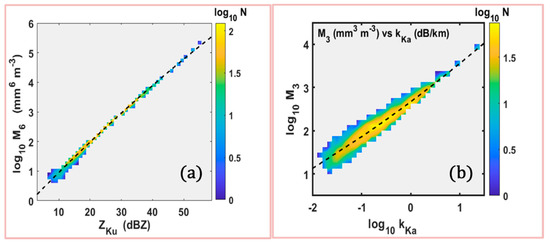
Figure 1.
(a) log10 (M6) versus ZKu and (b) log10 M3 versus kKa from simulations where the color scales represent the number of occurrences on a log scale. The dashed lines represent the fitted Equations (7) and (8).
The dashed lines in Figure 1a,b represent the fitted equations based on second-order polynomial equations:
where Zku is in dBZ units in Equation (8a). The fitted coefficients and their standard errors are given in Table 1.

Table 1.
The fitted coefficients to Equations (7) and (8) and their standard errors.
3.4. Stability of the Underlying DSD Shape
Next, we consider the uncertainties associated with the underlying shape of the DSDs using Equations (2)–(4). Figure 2a,b show the double-moment normalization (i.e., h(x) versus x) applied to the Greeley (GXY) and the Huntsville (HSV) datasets. In each case, the 25th, the 50th (median), and the 75th percentile curves are superimposed. The two sets of curves appear to be similar to each other.

Figure 2.
(a) log10 h(x) versus x as intensity color contoured plot from 3 min DSDs from GXY and (b) from HSV and the 25th, 50th (median), and 75th percentile curves overplotted; (c) the fitted values [μGG] versus c for all the GXY and HSV DSDs combined; (d) log10 h(x) versus x as intensity color contoured plot from 3 min DSDs during the outer-bands of category-1 Hurricane Dorian over Wallops together with the most-probable h(x) versus x constructed from (c).
Each of the 3 min DSDs from the GXY and HSV campaigns had been fitted to Equation (6) with i = 3 and j = 6 [53]. The fitted μGG versus c are shown in panel (c) as a color-intensity plot. μGG shows a narrow range, but the fitted c values range a wider span. Note, once again, that the color scale of N is on a log10 scale. The maximum value of N is reached for [μGG, c] = [−0.25, 3.67]. We will use these as the ‘most-probable’ combination and will substitute these values into Equation (6) for i = 3 and j = 6. To test this most-probable h(x), we show in panel (d) the color-intensity plot of h(x) versus x derived from the 3 min DSDs recorded during category-1 Hurricane Dorian (outer bands only) at the Wallops site [56] as well as the most-probable h(x) from the GXY-HSV analyses. The fit appears to be very representative, capturing the ‘high-intensity’ trend from the DSD data very well.
3.5. Simulations and Algorithm Errors
As seen in Section 3.3 and Section 3.4, our proposed retrieval method is expected to have uncertainties associated with each of the retrieved moments. To quantify these “algorithm errors”, forward simulations and retrievals were performed using the same set of 3 min DSDs from the three locations. Figure 3 shows the block-diagram for this procedure. The steps can be summarized as follows:

Figure 3.
Block diagram outlining the simulation procedure (top), and a comment regarding step (iii) in (bottom).
- i.
- Use the 3 min DSDs for scattering calculations at Ku and Ka bands;
- ii.
- Use the Zku and kka outputs from (i) to estimate M6 and M3 using Equations (7) and (8);
- iii.
- Retrieve the other moments, viz. M0, M1, M2, M4, M5, and M7, using the estimated [M3, M6] and h(x);
- iv.
- Calculate all moments [M0 … M7] using the same 3 min DSDs as in (i);
- v.
- Compare (iii) and (iv).
These steps are numbered in red in Figure 3. For step (iii) (with green-box outline), the retrieval of other moments can be achieved analytically using equation (42) of Lee et al. [18]; however, that expression is not valid when μGG is negative, which is the case for our h(x). An alternate solution is to estimate the other moments numerically by first constructing the full DSD spectra from each of the retrieved M3 and M6 in step (ii) and our h(x) with i = 3 and j = 4 for μGG = −0.25 and c = 3.67 in Equation (7). This is followed by the calculation of other moments using Equation (1).
Results from step (v) are shown in Figure 4 as scatterplots of the retrieved moments versus the ‘true’ moments, i.e., those derived directly from the 3 min DSDs. Only the cases with kKa > 1 dB/km were chosen. The 1:1 line is included in each plot. The higher-order moments, viz. M3 to M7 show very good correlation and lie close to the 1:1 line. The lower-order moments, especially M0, show more scatter. The errors are quantified in terms of the fractional standard error (FSE) in Table 2. They range from nearly 11% for M0 to just over 3% for M7, gradually decreasing. These values represent the overall algorithm errors of the retrieval method.

Figure 4.
Retrieved moments vs. those directly from the data, i.e., output of step (v) in Figure 3.
Table 2.
Fractional standard errors for the retrieval moments.
Algorithm errors are sometimes referred to as parameterization errors. Bringi et al. [31] considered an additional source of uncertainty, namely those due to radar measurement errors. They found that, for lower-order moments, the parameterization error dominates the overall uncertainties, whereas the radar-measurement errors dominate those for higher-order moments. Although their analyses were related to retrieval of moments from polarimetric radar data, the same trend is likely to apply for the DPR-based retrievals also. Next, we preform basic tests for our retrieval method for two GPM-DPR overpass cases.
4. GPM-DPR Overpass Cases
4.1. The Huntsville Event
The first of the two events considered here occurred over the Huntsville site, where the MPS and two 2DVDs had been installed ([53]; see also Section 3.2 earlier). It consisted of precipitation associated with a semi-organized line-convection on 11 April 2016, which moved across northern Alabama from ~17 to 24 h UTC. The line convection did not directly pass over the disdrometer site; instead, it was approximately 10 km to the west. The GPM-DPR overpass over the site occurred at 23:31 UTC.
The near-surface DPR products include measured and attenuation-corrected radar reflectivities both at Ka and Ku bands as well as Nw and Dm for each of the 4 km by 4 km radar pixels. The two quantities needed for our retrievals, as mentioned earlier, are the Ku-band radar reflectivity and the specific attenuation at Ka-band. The former is a ‘direct’ product, but of course, ZKu should be the reflectivity values after attenuation-correction is used. The latter, however, is not readily available, but on the other hand, it can be recreated by (i) utilizing Nw and Dm to derive the DSDs for each pixel, assuming the DPR assumption of standard gamma model with μ = 3, followed by (ii) T-matrix calculations to derive kKa for each of the DSDs. These are shown in panels (a) and (b) in Figure 5. In each panel, the color scale is included. The diamonds represent the location of the disdrometers in terms of latitude and longitude. Zku (attenuation-corrected) over the site was 34.6 dBZ, and kKa was 0.60 dB/km. The estimated M6 and M3 are shown in panels (c) and (d), respectively. The color scales (included within each panel) show the log10 of the moments. Using these two moments, together with the h(x) in Equation (6), the DSDs per pixel were derived, and the other moments, M0, M1, M2, M4, M5, and M7, were estimated. Four are shown in Figure 6.
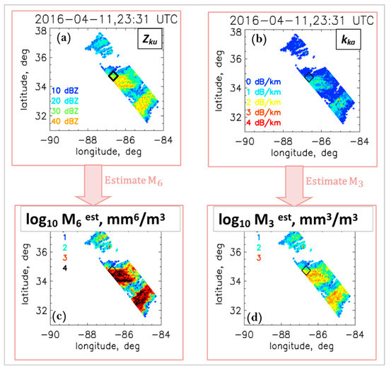
Figure 5.
DPR overpass over Huntsville on 11 April 2016 at 23:31 UTC. (a) Attenuation corrected ZKu; (b) Ka-band specific attenuation; (c) Estimated log10 (M6) from (a); (d) Estimated log10 (M3) from (b). Black diamonds indicate the disdrometer location.

Figure 6.
Examples of other retrieved moments for the 11 April 2016 case. (a) log10 (M1); (b) log10 (M2); (c) log10 (M4); (d) log10 (M5). Black Diamonds indicate the disdrometer location. The colors are the same as Figure 5.
Validation of the retrieved moments is not straightforward, but in Table 3, we show the mean and standard deviation of all moments M0 to M7 derived from the DPR data in (22) pixels over and surrounding the disdrometer site, which are compared with those derived directly from the (20) 3 min DSD within ±30 min time interval around the DPR overpass.
Table 3.
Mean and standard deviations of moments from DPR and DSDs on a log10 scale (units are mmn/m3 for nth moment) and the percentage errors.
From Table 3, we observe the following:
- i.
- Overall good agreement between the two sets of mean values, especially for the zeroth moment.
- ii.
- However, the DSD-based moments show somewhat lower mean values that the DPR-retrieved moments; although, when the standard deviations are included, the overlaps are considerable.
- iii.
- In both cases, M2 shows the lowest mean values and M7 the highest; the standard deviations also show a similar trend.
Furthermore, values of Dm, given by the ratio of the fourth moment to the third ranged from 0.9 to 1.8 mm for the DPR-based retrievals and 1.1 to 1.8 mm for the DSD-based estimates. The mean was 1.5 mm for both cases. Hence, it is likely that our retrievals of moments represent the ‘true’ values over the 4 km by 4 km pixel areas. Further comparisons are given in Appendix A.
4.2. Remnants of Storm Sally
The second event we consider in this paper is the remnants of Hurricane Sally over the Wallops area. This storm made landfall in the southern part of the US as category-1 hurricane but weakened considerably as it headed north-east. Remnants of this storm passed over the disdrometer location, and the GPM-DPR overpass occurred north of the site on 18 September 2020 at 04:40 UTC. The closest approach for the nadir beam was around 170 km NE of the disdrometer site, but the closest off-nadir beam was around 65 km north-east. Panel (a) in Figure 7 shows the (near-surface) attenuation-corrected ZKu, and panel (b) shows kKa. The retrieved M6 and M3 are shown in panels (c) and (d), respectively. These two moments were combined, as was done in the first event, with our most-probable h(x) to derive other moments. Two examples, namely M0 and M4, are shown in panels (e) and (f), respectively. Note the high M0 values in some regions, indicating high number concentrations.

Figure 7.
DPR overpass over Wallops during remnants of storm Sally. (a) Attenuation corrected ZKu; (b) Ka-band Specific Attenuation; (c) Estimated log10 (M6) from (a); (d) Estimated log10 (M3) from (b); (e) Estimated log10 (M0); (f) Estimated log10 (M4). The ‘diamond’ mark in panel (a) represents the disdrometer site.
Direct validation of the retrieved moments is, once again, not possible, especially because the DPR did not directly go over the disdrometer site, but in Figure 8, we compare the histograms of [M0 … M7] from DPR and the DSDs. For the latter, ±4 h around the DPR overpass time was used, whereas for the former, only the data shown in Figure 7 were used (a total of 3269 pixels). There seems considerable overlap in the two sets of histograms in all panels, but the DPR-based moments generally appear to be somewhat higher. On the other hand, if we restrict the DSD-based moment calculations to within 2 h of the DPR overpass, improvements in the agreement were observed. The green circle in each panel of Figure 8 represents the averaged value from the DSD data within the 2 h interval. They correspond very well to the mode of the DPR-based histograms.

Figure 8.
Storm Sally over Wallops area: Comparing histograms of log10 moments from DPR-retrieved moments (light red) and DSD based moments (light blue). The green circles represent the average of the DSD-based moments within a 2 h interval of the DPR overpass.
4.3. Evaluation of DSD Parameters
The two main DSD parameters often used in the radar retrievals are NW and Dm. There is also another parameter, namely the standard deviation of mass-spectrum, denoted as σM [37], considered useful for rain microphysics studies. While the first two parameters can be defined in terms of the third and the fourth moments, the third parameter additionally requires the fifth moment. The following equations can be derived:
Note, however, that Equation (11) is only valid for μGG > 0. For negative values, it is more appropriate to derive σM from the DSDs constructed using the two reference moments and the most-probable h(x).
Figure 9 compares histograms of DPR-retrieved and the DSD-based Dm and σM. Panel (a) corresponds to the HSV event and panel (b) to storm Sally over Wallops. There are clear differences between the two panels:

- i.
- Remnants of storm Sally shows narrower Dm histograms (both DPR-retrieved and DSD-based) having lower Dm values with a maximum value of only 1.6 mm whereas the whereas the HSV event shows Dm’s ranging up to 2.1 mm. This is to be expected, because storm Sally originated as a Hurricane, and it is well known that such storms contain an abundance of small drops (higher concentration) compared with other rain regimes [57,58].
- ii.
- The HSV event shows two peaks in the Dm, and these bimodal peaks are evident in both the DPR-retrieved and the DSD-based histograms. It is very plausible that the two peaks arise from the (semi-organized) line convection being embedded within a larger widespread (probably stratiform) rain region. The bimodal peaks are also noticeable in the σM histograms. Storm Sally, on the other hand, shows only one peak in both Dm and σM.
- iii.
- For the HSV event, there is considerable overlap between the DPR-retrieved and the DSD-based histograms, whereas for storm Sally, the DSD-based histogram has a higher number of cases with lower Dm values (i.e., <0.6 mm). This may well be due to the DPR sensitivity, which has a lower limit of approximately 12 dBZ for the radar reflectivity at Ku-band, which, in turn, indicates that light rainfall cases will not be detected often enough. On the other hand, the disdrometer-based DSDs include the MPS measurements with good accuracy for the concentration of small drops.
- iv.
- Another feature that is different between the two panels concerns the proportion of stratiform to convective rain. From the two clear peaks in Dm and σM histograms observed in the HSV event (as noted earlier in point (ii)), we can infer that the proportion of the two rain types are somewhat comparable. For storm Sally, by contrast, we have ascertained from NPOL radar quasi-vertical profiles (QVP; [59]) that it was largely stratiform rain. The single peak Dm histograms from both DPR and DSD data in panel (b) of Figure 9 support this.
Further improvement in the agreement between DPR and DSD histograms in Figure 9 may be obtained if we restrict the off-nadir angles for the DPR to be less than 10 degrees and/or by utilizing the ‘type_Precip’ flag product from DPR, in particular, the second digit of the flag. This will be investigated in the near future.
4.4. Evaluation of (Stratiform and Convective) Rain Types
Regarding stratiform and convective rain types, it is also of interest to examine the applicability of the classification based on Nw versus Dm separation technique. This observational-based empirical method has been used for disdrometer data in the past, and our own recent work has shown that the two rain types can be separated in the NW–Dm space [60,61,62]. The same method had also been applied to the S-band NPOL radar data and compared with a texture-based method described in [63]. Considerable agreement of over 86% was obtained [64]. Similar comparisons [65] were made for the C-band CPOL radar based in Darwin, Australia [66].
Disdrometer data represent “point-measurements” (albeit over a 1 or 3 min time interval), and ground-based radar data represent measurements over pulse volumes (but instantaneous). Despite these differences, the stratiform-convective rain separation technique seemed applicable to both. Here, we perform similar tests for the DPR-retrieved NW–Dm for the two cases, noting that the DPR footprint is much larger (4 km by 4 km) than the ground-based radar data.
The separation technique is based on whether a given pair of [NW, Dm] lies above or below or specified line. A simple index i given by the following equation is used to quantify the rain-type likelihood [64,65]:
where ‘sep’ corresponds to the separation line, and ‘est’ represents the estimated value.
Values of c1 and c2 may be location dependent, but to be consistent with our previous studies, we have used −1.682 and 6.541, respectively. Broadly speaking, when i is negative, stratiform rain is indicated, and when i is positive, convective rain is indicated. The pixel-by-pixel DPR-based index value derived for the HSV event is shown in panel (a) of Figure 10. The red color represents i > 0 (hence, convective rain regions), and the lighter colors indicate i < 0 (hence, stratiform rain regions). Panel (b) of Figure 10 shows the path integrated attenuation (PIA) from the matched scan (MS; [7]). The “diamond” symbol indicates the location of the disdrometer site. Positive values of i are seen south-east of the disdrometer site and correlate well, at least visually, with the PIA image in panel (b), i.e., the higher PIA regions correspond to positive index values (red) in panel (a).

Figure 10.
(a) Stratiform (blue) convective (red) rain likelihood index based on the NW versus Dm separation method for the 11 April 2016 event in HSV; (b) path-integrated attenuation from the matched scan. The diamond marks the disdrometer site.
Storm Sally, by contrast (as inferred earlier), was mostly stratiform rain when it passed over Wallops. Most of the DPR-retrieved index values (from Figure 7) were negative. Panel (a) of Figure 11 shows the variation of the index values with the PIA from the normal scan (NS; [7]) scan. Only data within a specified range of (off) nadir angles were used. Interestingly, one can see an increase in the i values with PIA. In other words, the NW–Dm points move closer to the separation line as the PIA increases, although they lie mostly on the stratiform rain side of the separation line. Panel (b) of Figure 11 shows the QVP plot (a conical scan at 20 deg elevation, height up to 10 km, and range of around 30 km) of the radar reflectivity from the S-band NPOL volume scans on 18 September 2020. The clear radar bright-band seen at 4–4.2 km height throughout the event confirms that the event was dominated by stratiform rain. This validates the predominantly negative i values from panel (c), which were derived from DPR-retrieved [NW, Dm]. The increase in i values with PIA in panel (a) is also consistent with another case event analyses using disdrometer data and vertically pointing X-band radar during a cold-rain event in Ontario, Canada (see Section 2 in Thurai et al. 2016), which showed an increase in the (negative values of) i with increasing bright-band thickness. Both the Ontario event analysis and the HSV event in Figure 11a show a very similar trend.
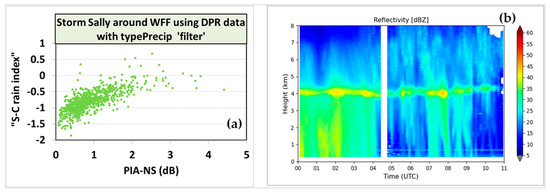
Figure 11.
(a) Stratiform–convective likelihood index based on the NW versus Dm separation method versus the path-integrated attenuation from the normal scan (PIA-NS) for the remnants of storm Sally in Wallops (note the index values are mostly negative indicating stratiform rain); (b) quasi-vertical profile of reflectivity from NPOL as time variation over the whole event, again indicating stratiform rain, from the dBZ bright-band in the 4–4.3 km a.m.s.l. throughout the event.
5. Summary and Discussion
Our results have shown that it is feasible to retrieve DSD moments directly from DPR-based quantities. The retrieved moments can act as an initial step, prior to deriving DSD parameters such as NW and Dm. Additionally, the DSD moments are very helpful in understanding the microphysical processes involved in various types of rain regimes. The basic premise of this article is that the lower order moments (M0, M2, M3) of the DSD, which are involved in the formulation of the warm rain process rates (such as evaporation, sedimentation, and binary collisions), can be expressed as products of power laws of the a priori chosen reference moments of higher order (M3, M6) along with moments of h(x), where h(x) is the intrinsic shape of the distribution. The form of h(x) can be any functional shape, provided its moments are finite and positive. The latter formulation also enables estimation of the standard deviation of the mass spectrum σM [67], as well as NW and Dm.
In our study, the retrieval of moments used only two DPR products, namely the attenuation-corrected radar reflectivity at Ku-band and the specific attenuation at Ka-band. They were used to retrieve the sixth (M6) and the third moments (M3), respectively. Using these two quantities as our chosen reference moments, and assuming an underlying shape function, h(x), for the DSDs, it is possible to retrieve other moments, ranging from M0 to M7. Note that h(x) is dependent on the pair of chosen moments, and we have assumed the generalized gamma model to represent h(x). Using 3000 3 min full DSD spectra from two (climatically) different locations, we found that the underlying function corresponding to [M3, M6] pair seemed reasonably stable.
Simulations using the 3000 3 min DSDs showed that the algorithm errors for the retrievals would be low; however, for lower-order moments, especially for M0, the errors were found to be more significant. When applying the technique to DPR data, other error sources also need to be considered. They include variance of radar measurement errors and ‘point-to-area’ variance, which arises from the fact that disdrometer data represent point measurements (although over a 3 min period), whereas DPR data are over a much larger footprint (although instantaneous), and factors such as non-uniform beam filling also need to be considered. We also need to bear in mind that the DPR has a lower threshold of around 12 dBZ for Ku-band measurements, which will put a lower limit of the estimated M6 used in this method.
Two GPM-DPR overpass cases were used to examine the validity of our retrieval technique, one over the Huntsville site on 11 April 2016 at 23:31 UTC and one over the Wallops site on 18 September 2020 at 04:42 UTC during the passage of remnants of storm Sally. We compared the mean and standard deviation of all moments (M0 to M7) derived from the DPR data in pixels in the 0.05 degree of latitude and 0.05 degree longitude around the disdrometer site and compared them with those derived directly from the DSD within a 30 min time interval around the DPR overpass. The agreement for all moments (in terms of log10) was well within 10%. Furthermore, values of Dm, given by the ratio of the fourth moment to the third, ranged from 0.9 to 1.8 mm for the DPR-based retrievals around the disdrometer site and 1.1 to 1.8 mm for the DSD-based estimates over a ±30 min period. For the second case, histograms of the moments were derived from DPR and DSDs, and when the DPR-based moments were restricted to areas over and surrounding the disdrometer location, their modes showed very good agreement with the DSD-based mean values, which determined when the disdrometer data were restricted to within 2 h of the DPR overpass.
Dm and σM histograms were also compared for both events. Of the two, remnants of hurricane Sally showed narrower Dm histograms, both DPR-retrieved and DSD-based, having lower Dm values with a maximum value of only 1.6 mm, whereas the HSV event shows Dm values ranging up to 2.1 mm. The latter, in fact, showed two peaks in the Dm, and these bimodal peaks are evident in both the DPR-retrieved and the DSD-based histograms. They were attributed to the semi-organized convective line being embedded within a larger widespread (and seemingly stratiform) rain region. The bimodal peaks were also noticeable in the σM histograms. Sally (around the Wallops disdrometer area), on the other hand, shows only one peak in both Dm and σM. The tropical environment may also be the reason that no larger drop mode was observed by the disdrometers or DPR.
Finally, a previously published method for separating stratiform and convective rain types was tested for the two events. The method is based on Nw versus Dm and has been tested using disdrometer data in several locations, e.g., [60,61,62], and against the texture-based method used in [63]. For the two events considered here, the DPR-based NW versus Dm (again note considerably larger footprint) were used to identify regions of the two rain types. For the HSV event, the convective rain regions corresponded well with regions of high PIA from the matched scan. On the other hand, DPR data for Sally showed mostly stratiform rain during the overpass. This was confirmed by QVP constructed from NPOL radar for the event.
The two initial test cases show encouraging results for more informative and accurate DSD retrievals from DPR. Our retrieval method for DSD moments followed a procedure similar to previous work by Bringi et al. [31], using X-band ground-based polarimetric radar data. The third and the sixth moments had also been used for that study. It is likely that these are also applicable for the DPR based retrievals, but further investigations are needed. Another aspect to consider is the stability of h(x), specifically, whether having two sets of h(x), one for stratiform rain and one for convective rain would improve the overall retrievals. This will also be examined in the future.
The novelty of our method lies in the conceptual fact that the rain DSDs are better characterized in terms of moments rather than the DSD parameters governing the distributions. As mentioned earlier in the Introduction, DSD moments are far more informative about the microphysical processes involved in the observation regions. Given that the DPR is capable of providing vertical profiles of attenuation corrected radar reflectivities as well as specific attenuations at Ku and Ka bands, the height variations of the DSD moments will lead to better understanding of the dominant processes. One drawback to our method is that the Ka-band specific attenuation, as mentioned several times earlier, has not been made available as one of the ‘official DPR products’. It is hoped that this will be included in the near future. The specific attenuation can also be used as one of the rain-rate estimators, as has been the base for S-band ground-based radars [68] as well as X-band ground-based radars [69].
Author Contributions
Conceptualization, M.T. and V.B.; Methodology, Investigation, and Formal Analysis, M.T. and V.B.; Data Curation, D.A.M. and M.T.W.; Writing—Original Draft Preparation, M.T. and V.B.; Writing—Review and Editing, P.N.G. and D.W.; Supervision, V.B., P.N.G. and D.W.; Resources, D.W. All authors have read and agreed to the published version of the manuscript.
Funding
M.T. was funded by NASA’s Precipitation Measurement Mission via Grant Award Number 80NSSC19K0676. V.B. was funded by NASA Atmospheric Dynamics program via Grant Award Number 80NSSC20K0893.
Data Availability Statement
Data can be made available upon request to any of the authors.
Acknowledgments
We wish to thank the four anonymous reviewers for their helpful comments.
Conflicts of Interest
The authors declare no conflict of interest. The funders had no role in the design of this study; in the collection, analyses, or interpretation of its data; in the writing of this manuscript, and in the decision to publish these results.
Appendix A
For the Huntsville event considered in Section 4.1, histograms of the retrieved DSD moments are shown in Figure A1 in this Appendix. The histograms were derived for all pixels (60) over and surrounding the disdrometer location. The latitude and longitude range are as follows:
- Latitude (deg) … from 34.999 to 34.3029
- Longitude (deg) … from −86.0023 to −86.9818
- Location of the disdrometers: 34.7245° (lat) −86.6398° (lon)
The arrows in maroon color on top of each panel correspond to the range of values determined from the ground-based 3 min DSDs from 23:00 to 24:00 UTC, i.e., within ±30 min period of the DPR overpass time of 23:31 UTC. Reasonable agreement is seen for the lower order moments, viz. M0, M1, and M2, as well as the higher-order moments, viz. M6 and M7. For those in the middle, i.e., M3, M4, and M5, there appears to be a slight overestimate of the values estimated from DPR. Overall, however, the range of DSD-based values lie well withing the range of the corresponding moments. The mean values from the DSD-based moments are provided above each panel.
As a further “sanity check”, in Figure A2, we show (in green) the actual DSDs constructed from the retrieved from the DPR data from the abovementioned pixels. Overplotted in maroon are the DSD measurements from the 2DVD and MPS disdrometers over the same ±30 min period of the DPR overpass time of 23:31 UTC. The DSD measurements show less variability than the DPR-based DSDs, particularly at the larger sizes, but they mostly lie within the set of green curves.

Figure A1.
Histograms of moments (units are mmn/m3 for the nth moment) shown in green derived from DPR data over and around the disdrometer site for the 11 April 2016 event in Huntsville (Figure 5). The maroon arrows represent those derived from the ground-based DSD measurements within ±30 min period around the overpass time.


Figure A2.
DSDs shown in green reconstructed from the moments in Figure A1 and those from the ground measurements in maroon.
Figure A2.
DSDs shown in green reconstructed from the moments in Figure A1 and those from the ground measurements in maroon.

References
- Hou, A.Y.; Kakar, R.K.; Neeck, S.; Azarbarzin, A.A.; Kummerow, C.D.; Kojima, M.; Oki, R.; Nakamura, K.; Iguchi, T. The Global Precipitation Measurement Mission. Bull. Am. Meteorol. Soc. 2014, 95, 701–722. [Google Scholar] [CrossRef]
- Seto, S.; Iguchi, T.; Oki, T. The Basic Performance of a Precipitation Retrieval Algorithm for the Global Precipitation Measurement Mission’s Single/Dual-Frequency Radar Measurements. IEEE Trans. Geosci. Remote Sens. 2013, 51, 5239–5251. [Google Scholar] [CrossRef]
- Gao, J.; Tang, G.; Hong, Y. Similarities and Improvements of GPM Dual-Frequency Precipitation Radar (DPR) upon TRMM Precipitation Radar (PR) in Global Precipitation Rate Estimation, Type Classification and Vertical Profiling. Remote Sens. 2017, 9, 1142. [Google Scholar] [CrossRef]
- Adirosi, E.; Montopoli, M.; Bracci, A.; Porcù, F.; Capozzi, V.; Annella, C.; Budillon, G.; Bucchignani, E.; Zollo, A.L.; Cazzuli, O.; et al. Validation of GPM Rainfall and Drop Size Distribution Products through Disdrometers in Italy. Remote Sens. 2021, 13, 2081. [Google Scholar] [CrossRef]
- Testud, J.; Oury, S.; Black, R.A.; Amayenc, P.; Dou, X. The concept of “normalized” distribution to describe raindrop spectra: A tool for cloud physics and cloud remote sensing. J. Appl. Meteorol. 2001, 40, 1118–1140. [Google Scholar] [CrossRef]
- Liao, L.; Meneghini, R. Physical Evaluation of GPM DPR Single- and Dual-Wavelength Algorithms. J. Atmos. Ocean. Technol. 2019, 36, 883–902. [Google Scholar] [CrossRef]
- Iguchi, T.; Seto, S.; Meneghini, R.; Yoshida, N.; Awaka, J.; Le, M.; Chandrasekar, V.; Brodzik, S.; Kubota, T. GPM/DPR Level-2 Algorithm Theoretical Basis Document Version 6; NASA Goddard Space Flight Ceneter: Greenbelt, MA, USA, 2018.
- Seto, S.; Iguchi, T.; Meneghini, R.; Awaka, J.; Kubota, T.; Masaki, T.; Takahashi, N. The Precipitation Rate Retrieval Algorithms for the GPM Dual-frequency Precipitation Radar. J. Meteorol. Soc. Jpn. Ser. II 2021, 99, 2021-011. [Google Scholar] [CrossRef]
- Gatlin, P.N.; Petersen, W.A.; Pippitt, J.L.; Berendes, T.A.; Wolff, D.B.; Tokay, A. The GPM Validation Network and Evaluation of Satellite-Based Retrievals of the Rain Drop Size Distribution. Atmosphere 2020, 11, 1010. [Google Scholar] [CrossRef]
- Radhakrishna, B.; Satheesh, S.K.; Rao, T.N.; Saikranthi, K.; Sunilkumar, K. Assessment of DSDs of GPM-DPR with ground-based disdrometer at seasonal scale over Gadanki, India. J. Geophys. Res. Atmos. 2016, 121, 11792–11802. [Google Scholar] [CrossRef]
- Ryu, J.; Song, H.-J.; Sohn, B.-J.; Liu, C. Global Distribution of Three Types of Drop Size Distribution Representing Heavy Rainfall From GPM/DPR Measurements. Geophys. Res. Lett. 2021, 48, e2020GL090871. [Google Scholar] [CrossRef]
- Hamada, A.; Takayabu, Y.N. Improvements in detection of light precipitation with the global precipitation measurement dual-frequency precipitation radar (GPM DPR). J. Atmos. Ocean. Technol. 2016, 33, 653–667. [Google Scholar] [CrossRef]
- Tuttle, J.D.; Rinehart, R.E. Attenuation Correction in Dual-Wavelength Analyses. J. Appl. Meteorol. Climatol. 1983, 22, 1914–1921. [Google Scholar] [CrossRef][Green Version]
- Fujita, M. An algorithm for estimating rain rate by a dual-frequency radar. Radio Sci. 1983, 18, 697–708. [Google Scholar] [CrossRef]
- Eccles, P.J. Comparison of Remote Measurements by Single- and Dual-Wavelength Meteorological Radars. IEEE Trans. Geosci. Electron. 1979, 17, 205–218. [Google Scholar] [CrossRef]
- Walker, B.; Lamberth, L.S.; Stephens, J.J. Dual-Frequency Radar Observations of Precipitation. J. Appl. Meteorol. Climatol. 1964, 3, 430–438. [Google Scholar] [CrossRef][Green Version]
- Ellis, S.M.; Vivekanandan, J. Liquid water content estimates using simultaneous S and Ka band radar measurements. Radio Sci. 2011, 46, RS2021. [Google Scholar] [CrossRef]
- Lee, G.; Zawadzki, I.; Szyrmer, W.; Sempere-Torres, D.; Uijlenhoet, R. A general approach to double-moment normalization of drop size distributions. J. Appl. Meteorol. 2004, 43, 264–281. [Google Scholar] [CrossRef]
- Atlas, D.; Ulbrich, C.W. Path- and Area-Integrated Rainfall Measurement by Microwave Attenuation in the 1–3 cm Band. J. Appl. Meteorol. Climatol. 1977, 16, 1322–1331. [Google Scholar] [CrossRef]
- Bringi, V.; Grecu, M.; Protat, A.; Thurai, M.; Klepp, C. Measurements of Rainfall Rate, Drop Size Distribution, and Variability at Middle and Higher Latitudes: Application to the Combined DPR-GMI Algorithm. Remote Sens. 2021, 13, 2412. [Google Scholar] [CrossRef]
- Milbrandt, J.A.; McTaggart-Cowan, R. Sedimentation-Induced Errors in Bulk Microphysics Schemes. J. Atmos. Sci. 2010, 67, 3931–3948. [Google Scholar] [CrossRef]
- Bryan, G.H.; Morrison, H. Sensitivity of a Simulated Squall Line to Horizontal Resolution and Parameterization of Microphysics. Mon. Weather Rev. 2012, 140, 202–225. [Google Scholar] [CrossRef]
- Jameson, A.R. The Meteorological Parameterization of Specific Attenuation and Polarization Differential Phase Shift in Rain. J. Appl. Meteorol. 1993, 32, 1741–1750. Available online: http://www.jstor.org/stable/44713974 (accessed on 19 November 2021). [CrossRef]
- Milbrandt, J.A.; Yau, M.K. A Multi-moment Bulk Microphysics Parameterization. Part I: Analysis of the Role of the Spectral Shape Parameter. J. Atmos. Sci. 2005, 62, 3051–3064. [Google Scholar] [CrossRef]
- Prat, O.P.; Barros, A.P.; Williams, C.R. an intercomparison of model simulations and VPR estimates of the vertical structure of warm stratiform rainfall during TWP-ICE. J. Appl. Meteorol. Climatol. 2008, 47, 2797–2815. [Google Scholar] [CrossRef]
- Morrison, H.; Kumjian, M.R.; Martinkus, C.P.; Prat, O.P.; Van Lier-Walqui, M. A general N-moment normalization method for deriving raindrop size distribution scaling relationships. J. Appl. Meteorol. Climatol. 2019, 58, 247–267. [Google Scholar] [CrossRef]
- Morrison, H.; van Lier-Walqui, M.; Kumjian, M.R.; Prat, O.P. A Bayesian Approach for Statistical-Physical Bulk Parameterization of Rain Microphysics. Part I: Scheme Description. J. Atmos. Sci. 2020, 77, 1019–1041. [Google Scholar] [CrossRef]
- Szyrmer, W.; Laroche, S.; Zawadzki, I. A Microphysical Bulk Formulation Based on Scaling Normalization of the Particle Size Distribution. Part I: Description. J. Atmos. Sci. 2005, 62, 4206–4221. [Google Scholar] [CrossRef]
- Meneghini, R.; Liao, L. On the Equivalence of Dual-Wavelength and Dual-Polarization Equations for Estimation of the Raindrop Size Distribution. J. Atmos. Ocean. Technol. 2007, 24, 806–820. [Google Scholar] [CrossRef][Green Version]
- Raupach, T.H.; Berne, A. Retrieval of the raindrop size distribution from polarimetric radar data using double-moment normalization. Atmos. Meas. Tech. 2017, 10, 2573–2594. [Google Scholar] [CrossRef]
- Bringi, V.; Mishra, K.V.; Thurai, M.; Kennedy, P.C.; Raupach, T.H. Retrieval of lower-order moments of the drop size distribution using CSU-CHILL X-band polarimetric radar: A case study. Atmos. Meas. Tech. 2020, 13, 4727–4750. [Google Scholar] [CrossRef]
- Raupach, T.H.; Berne, A. Invariance of the double-moment normalized raindrop size distribution through 3D spatial displacement in stratiform rain. J. Appl. Meteorol. Climatol. 2017, 56, 1663–1680. [Google Scholar] [CrossRef]
- Thurai, M.; Bringi, V.; Gatlin, P.N.; Petersen, W.A.; Wingo, M.T. Measurements and modeling of the full rain drop size distribution. Atmosphere 2019, 10, 39. [Google Scholar] [CrossRef]
- Marshall, J.S.; Palmer, W.M.K. The distribution of raindrops with size. J. Meteorol. 1948, 5, 165–166. [Google Scholar] [CrossRef]
- Ulbrich, C.W. Natural Variations in the Analytical Form of the Raindrop Size Distribution. J. Clim. Appl. Meteorol. 1983, 22, 1764–1775. [Google Scholar] [CrossRef]
- Kozu, T.; Iguchi, T.; Shimomai, T.; Kashiwagi, N. Raindrop size distribution modeling from a statistical rain parameter relation and its application to the TRMM precipitation radar rain retrieval algorithm. J. Appl. Meteorol. Climatol. 2009, 48, 716–724. [Google Scholar] [CrossRef]
- Williams, C.R.; Bringi, V.N.; Carey, L.D.; Chandrasekar, V.; Gatlin, P.N.; Haddad, Z.S.; Meneghini, R.; Munchak, S.J.; Nesbitt, S.W.; Petersen, W.A.; et al. Describing the Shape of Raindrop Size Distributions Using Uncorrelated Raindrop Mass Spectrum Parameters. J. Appl. Meteorol. Climatol. 2014, 53, 1282–1296. [Google Scholar] [CrossRef]
- Mallet, C.; Barthes, L. Estimation of gamma raindrop size distribution parameters: Statistical fluctuations and estimation errors. J. Atmos. Ocean. Technol. 2009, 26, 1572–1584. [Google Scholar] [CrossRef]
- Sekhon, R.; Srivastava, R.C. Doppler Radar Observations of Drop-Size Distributions in a Thunderstorm. J. Atmos. Sci. 1971, 28, 983–994. [Google Scholar] [CrossRef]
- Bringi, V.N.; Chandrasekar, V. Polarimetric Doppler Weather Radar: Principles and Applications; Cambridge University Press: Cambridge, UK, 2001. [Google Scholar]
- Ryzhkov, A.; Zrnic, D.S. Radar Polarimetry for Weather Observations; Springer: Cham, Switzerland, 2019. [Google Scholar]
- Nakamura, K.; Iguchi, T. Dual-wavelength radar algorithm. In Measuring Precipitation from Space; Levizanni, V., Bauer, P., Turk, F.J., Eds.; Springer: Dordrecht, The Netherlands, 2007; pp. 225–234. [Google Scholar]
- Skofronick-Jackson, G.; Kirschbaum, D.; Petersen, W.; Huffman, G.; Kidd, C.; Stocker, E.; Kakar, R. The Global Precipitation Measurement (GPM) mission’s scientific achievements and societal contributions: Reviewing four years of advanced rain and snow observations. Q. J. R. Meteorol. Soc. 2018, 144, 27–48. [Google Scholar] [CrossRef] [PubMed]
- Sempere-Torres, D.; Porrà, J.M.; Creutin, J.-D. Experimental evidence of a general description for raindrop size distribution properties. J. Geophys. Res. 1998, 103, 1785–1797. [Google Scholar] [CrossRef]
- Illingworth, A.J.; Blackman, T.M. The Need to Represent Raindrop Size Spectra as Normalized Gamma Distributions for the Interpretation of Polarization Radar Observations. J. Appl. Meteorol. 2002, 41, 286–297. [Google Scholar] [CrossRef]
- Yu, N.; Delrieu, G.; Boudevillain, B.; Hazenberg, P.; Uijlenhoet, R. Unified Formulation of Single- and Multimoment Normalizations of the Raindrop Size Distribution Based on the Gamma Probability Density Function. J. Appl. Meteorol. Climatol. 2014, 53, 166–179. Available online: http://www.jstor.org/stable/26175953 (accessed on 18 November 2021). [CrossRef]
- Auf der Maur, A.N. Statistical tools for drop size distributions: Moments and generalized gamma. J. Atmos. Sci. 2001, 58, 407–418. [Google Scholar] [CrossRef]
- Baumgardner, D.; Kok, G.; Dawson, W.; O’Connor, D.; Newton, R. A new ground-based precipitation spectrometer: The Meteorological Particle Sensor (MPS). In Proceedings of the 11th Conference on Cloud Physics, Ogden, UT, USA, 2–3 June 2002; p. 8.6. [Google Scholar]
- Schoenhuber, M.; Lammer, G.; Randeu, W.L. One decade of imaging precipitation measurement by 2D-video-distrometer. Adv. Geosci. 2007, 10, 85–90. [Google Scholar] [CrossRef]
- Schönhuber, M.; Lammer, G.; Randeu, W.L. The 2D-Video-Distrometer. In Precipitation: Advances in Measurement, Estimation and Prediction; Michaelides, S., Ed.; Springer: Berlin/Heidelberg, Germany, 2008; pp. 3–31. ISBN 978-3-540-77654-3. [Google Scholar]
- Rasmussen, R.; Baker, B.; Kochendorfer, J.; Meyers, T.; Landolt, S.; Fischer, A.P.; Black, J.; Thériault, J.M.; Kucera, P.; Gochis, D.; et al. How Well Are We Measuring Snow: The NOAA/FAA/NCAR Winter Precipitation Test Bed. Bull. Am. Meteorol. Soc. 2012, 93, 811–829. [Google Scholar] [CrossRef]
- Raupach, T.H.; Thurai, M.; Bringi, V.N.; Berne, A. Reconstructing the Drizzle Mode of the Raindrop Size Distribution Using Double-Moment Normalization. J. Appl. Meteorol. 2019, 58, 145–164. [Google Scholar] [CrossRef]
- Thurai, M.; Gatlin, P.N.; Bringi, V.N.; Petersen, W.A.; Notaros, B.; Carey, L.D.; Kennedy, P. Towards completing the rain drop size spectrum: Case studies involving 2D-video disdrometer, droplet spectrometer, and polarimetric radar measurements. J. Appl. Meteorol. Climatol. 2017, 56, 877–896. [Google Scholar] [CrossRef]
- Bringi, V.; Seifert, A.; Wu, W.; Thurai, M.; Huang, G.-J.; Siewert, C. Hurricane Dorian Outer Rain Band Observations and 1D Particle Model Simulations: A Case Study. Atmosphere 2020, 11, 879. [Google Scholar] [CrossRef]
- Mishchenko, M.I.; Travis, L.D.; Mackowski, D.W. T-matrix computations of light scattering by nonspherical particles: A review. J. Quant. Spectrosc. Radiat. Transf. 1996, 55, 535–575. [Google Scholar] [CrossRef]
- Thurai, M.; Bringi, V.N.; Wolff, D.B.; Marks, D.A.; Pabla, C.S. Drop Size Distribution Measurements in Outer Rainbands of Hurricane Dorian at the NASA Wallops Precipitation-Research Facility. Atmosphere 2020, 11, 578. [Google Scholar] [CrossRef]
- Brown, B.R.; Bell, M.M.; Frambach, A.J. Validation of simulated hurricane drop size distributions using polarimetric radar. Geophys. Res. Lett. 2016, 43, 910–917. [Google Scholar] [CrossRef]
- Wolff, D.B.; Petersen, W.A.; Tokay, A.; Marks, D.A.; Pippitt, J.L. Assessing Dual-Polarization Radar Estimates of Extreme Rainfall during Hurricane Harvey. J. Atmos. Ocean. Technol. 2019, 36, 2501–2520. [Google Scholar] [CrossRef]
- Ryzhkov, A.V.; Zhang, P.; Reeves, H.; Kumjian, M.; Tschallener, T.; Tromel, S.; Simmer, C. Quasi-Vertical Profiles—A new way to look at polarimetric radar data. J. Atmos. Ocean. Technol. 2016, 33, 551–562. [Google Scholar] [CrossRef]
- Bringi, V.N.; Williams, C.R.; Thurai, M.; May, P.T. Using dual-polarized radar and dual-frequency profiler for DSD characterization: A case study from Darwin, Australia. J. Atmos. Ocean. Technol. 2009, 26, 2107–2122. [Google Scholar] [CrossRef]
- Thurai, M.; Gatlin, P.N.; Bringi, V.N. Separating stratiform and convective rain types based on the drop size distribution characteristics using 2D video disdrometer data. Atmos. Res. 2016, 169 Pt B, 416–423. [Google Scholar] [CrossRef]
- Thurai, M.; Bringi, V.; Wolff, D.; Marks, D.; Pabla, C. Testing the Drop-Size Distribution-Based Separation of Stratiform and Convective Rain Using Radar and Disdrometer Data from a Mid-Latitude Coastal Region. Atmosphere 2021, 12, 392. [Google Scholar] [CrossRef]
- Steiner, M.; Houze, R.A.; Yuter, S.E. Climatological Characterization of Three-Dimensional Storm Structure from Operational Radar and Rain Gauge Data. J. Appl. Meteor. 1995, 34, 1978–2007. [Google Scholar] [CrossRef]
- Thurai, M.; Wolff, D.; Marks, D.; Pabla, C.; Bringi, V. Separation of Stratiform and Convective Rain Types Using Data from an S-Band Polarimetric Radar: A Case Study Comparing Two Different Methods. Environ. Sci. Proc. 2021, 8, 1. [Google Scholar] [CrossRef]
- Thurai, M.; Bringi, V.N.; May, P.T. CPOL radar-derived drop size distribution statistics of stratiform and convective rain for two regimes in Darwin, Australia. J. Atmos. Ocean. Technol. 2010, 27, 932–942. [Google Scholar] [CrossRef]
- Penide, G.; Kumar, V.; Protat, A.; May, P.T. Statistics of drop size distribution parameters and rain rates for stratiform and convective precipitation during the north Australian wet season. Mon. Weather Rev. 2013, 141, 3222–3237. [Google Scholar] [CrossRef]
- Haddad, Z.S.; Short, D.A.; Durden, S.L.; Im, E.; Hensley, S.; Grable, M.B.; Black, R.A. A new parametrization of the rain drop size distribution. IEEE Trans. Geosci. Remote Sens. 1997, 35, 532–539. [Google Scholar] [CrossRef]
- Ryzhkov, A.V.; Diederich, M.; Zhang, P.; Simmer, C. Potential utilization of specific attenuation for rainfall estimation, mitigation of partial beam blockage, and radar networking. J. Atmos. Ocean. Technol. 2014, 31, 599–619. [Google Scholar] [CrossRef]
- Thurai, M.; Mishra, K.V.; Bringi, V.N.; Krajewski, W. Initial Results of a New Composite-Weighted Algorithm for Dual-Polarized X-Band Rainfall Estimation. J. Hydrometeorol. 2017, 18, 1081–1100. [Google Scholar] [CrossRef]


Publisher’s Note: MDPI stays neutral with regard to jurisdictional claims in published maps and institutional affiliations. |
© 2021 by the authors. Licensee MDPI, Basel, Switzerland. This article is an open access article distributed under the terms and conditions of the Creative Commons Attribution (CC BY) license (https://creativecommons.org/licenses/by/4.0/).