Investigating the Effects of k and Area Size on Variance Estimation of Multiple Pixel Areas Using a k-NN Technique for Forest Parameters

Abstract

Combining auxiliary variables and field inventory data of forest parameters using the model-based approach is frequently used to produce synthetic estimates for small areas. These small areas arise when it may not be financially feasible to take ground measurements or when such areas are inaccessible. Until recently, these estimates have been calculated without providing a measure of the variance when aggregating multiple pixel areas. This paper uses a Random Forest algorithm to produce estimates of quadratic mean diameter at breast height (QMDBH) (cm), basal area (m${}^2$ ha${}^{-1}$), stem density (n/ha${}^{-1}$), and volume (m${}^3$ ha${}^{-1}$), and subsequently estimates the variance of multiple pixel areas using a k-NN technique. The area of interest (AOI) is the state owned commercial forests in the Slieve Bloom mountains in the Republic of Ireland, where the main species are Sitka spruce (Picea sitchensis (Bong.) Carr.) and Lodgepole pine (Pinus contorta Dougl.). Field plots were measured in summer 2018 during which a lidar campaign was flown and Sentinel 2 satellite imagery captured, both of which were used as auxiliary variables. Root mean squared error (RMSE%) and R${}^2$ values for the modelled estimates of QMDBH, basal area, stem density, and volume were 19% (0.70), 22% (0.67), 28% (0.62), and 26% (0.77), respectively. An independent dataset of pre-harvest forest stands was used to validate the modelled estimates. A comparison of measured values versus modelled estimates was carried out for a range of area sizes with results showing that estimated values in areas less than 10–15 ha in size exhibit greater uncertainty. However, as the size of the area increased, the estimated values became increasingly analogous to the measured values for all parameters. The results of the variance estimation highlighted: (i) a greater value of k was needed for small areas compared to larger areas in order to obtain a similar relative standard deviation (RSD) and (ii) as the area increased in size, the RSD decreased, albeit not indefinitely. These results will allow forest managers to better understand how aspects of this variance estimation technique affect the accuracy of the uncertainty associated with parameter estimates. Utilising this information can provide forest managers with inventories of greater accuracy, therefore ensuring a more informed management decision. These results also add further weight to the applicability of the k-NN variance estimation technique in a range of forests landscapes.

1. Introduction

Sample surveys have been able to provide estimates of finite population totals and means since 1901 [1]. However, more detailed estimates for specific areas of interest are frequently desired. These areas can be described as small areas which has been defined as “any domain for which direct estimates of adequate precision cannot be produced” [2], such as when intensive field plot sampling is not financially feasible or where areas are not accessible. Two widely accepted methods for small area estimation (SAE) are probability-based model-assisted inference and model-based inference, both methods use models to estimate target variables for small areas but differ in their sources of randomness [3]. Probability-based model-assisted inference: (i) regards the sample as fixed, (ii) regards the sample as randomly generated, and (iii) considers that the source of randomness is due to the sampling method [3]. In contrast, model-based inference: (i) regards the sample as random even if it has not been randomly selected, however, to ensure the more appropriate model is created, a random selection should be used [4]; (ii) the observations are regarded as a realisation of random variables [4]; (iii) considers that the source of randomness is due to the population; and (iv) depends completely on the ability of the model to describe the real world [5]. This difference in assumptions means that probability samples for model-based inferences are not needed. Small area estimates using model-based inference are considered synthetic, as they only use the predicted values and do not incorporate model errors [2]. Updating forest inventory has advanced considerably with the improvements of technology, especially over the past 20–30 years, due to the advantages of using earth observation (EO) data as auxiliary variables for small area estimation [6,7].

One technique of model-based inference in forest inventory, called the area-based approach (ABA), has proved to be very useful in modelling ground data and EO auxiliary variables [6]. This approach consists of (i) Stand delineation: the forest stands within the area of interest (AOI) are delineated, (ii) field survey: a field survey is carried out within the AOI, (iii) remote sensing: remotely sensed data is acquired and processed for the AOI, (iv) modelling: regression models fit the field plot data and ALS metrics, and (v) stand-wise estimation: the fitted models and auxiliary variables are used to estimate parameters of interest for every grid cell [7]. Although originally implemented using satellite imagery as the auxiliary variables [6,8], the methodology can also be used with Light Detection and Ranging (lidar) data. Since its first application, the methodology has been used in a variety of landscapes to model a range of parameters such as mean tree height, mean diameter at breast height (dbh), biomass, stem density, basal area, and volume [9,10,11,12,13,14,15,16,17,18]. Despite the fact that these estimates are extremely useful to forest managers, due to the potential of updating large scale forest inventories without the need for intensive sampling, they provide no estimate for the associated variance. It is therefore crucial that the forest manager has both an estimate of the parameter of interest and the associated variance in order to have an updated inventory to make informed management decisions from.

The variance associated with volume was first estimated by comparing a non-parametric and parametric estimator [19], followed by a logistic regression methodology that incorporated spatial correlation between pixel estimates [20]. This was further developed by using a k-NN technique that calculated parametric estimators for ${\sigma }_i^2$ and Var ($\widehat{\mu }$) that accommodate spatial correlation among reference set observations [13]. It also incorporates the uncertainty associated with spatial correlation and allows for variance estimates for multiple pixel AOIs. Prior to this, in 2007, variance estimates for multiple pixel AOI’s had not been reported and to date, and few studies have implemented it. The investigation estimated the variance of volume (m³ ha⁻¹), basal area (m² ha⁻¹), stem density, and the proportion of forested area of 15 circular AOIs, each with a 10 km radius in Minnesota, United States of America, using satellite imagery. These AOIs are naturally regenerated hardwoods and conifers such as aspen, birch, spruce, and fir mixtures. The results indicated that this k-NN technique did not lose precision relative to the probability-based approach, which is usually implemented for forest inventory.

In Ireland, previous research has focused on utilising the ABA and satellite imagery utilising Random Forest and k-NN models to estimate basal area (RMSE 10.8–16.6 m${}^2$ ha${}^{-1}$) and volume (RMSE 104–158 m${}^3$ ha${}^{-1}$) [21]. Other investigations implemented an improved k-NN model to estimate basal area (RMSE 15–19 m${}^2$ ha${}^{-1}$) and volume (128 m${}^3$ ha${}^{-1}$ to 150 m${}^3$ ha${}^{-1}$) [18]. Both of these studies have analysed forest parameters at a national scale incorporating the National Forest Inventories to produce estimates. More recently, research has focused on simulating field plots of forest parameters. This involved the simulation of 100 plots using the Discrete Anisotropic Radiative Transfer (DART) model with discrete-return height distributions. The results produced excellent estimates for basal area (RMSE 1.7 m${}^2$ ha${}^{-1}$, RMSE% 5.4%, Pearson correlation coefficient value of 0.995) and mean DBH (RMSE 1.4 cm, RMSE% 7.3%, Pearson correlation coefficient value of 0.990) [22]. These results can be used to simulate a validation dataset which would reduce the costs associated with field inventory.

This paper utilises these advances, specifically the ability to obtain variance estimates of multiple pixel AOIs, which are not widely reported in the literature, to investigate the effects the k value and the size of an AOI has on variance estimation. This is explored by modelling four parameters, QMDBH, basal area, stem density, and volume of state owned forests in the Slieve Bloom mountains in the Republic of Ireland. Each parameter will be estimated using two machine learning algorithms independently—random forest and k-NN—and implement the methodology employed by [13], and further described in the initial description in [23], to calculate the variance of these areas. The variance is calculated using a k-NN technique, which is separate from the modelling process.

2. Materials and Methods

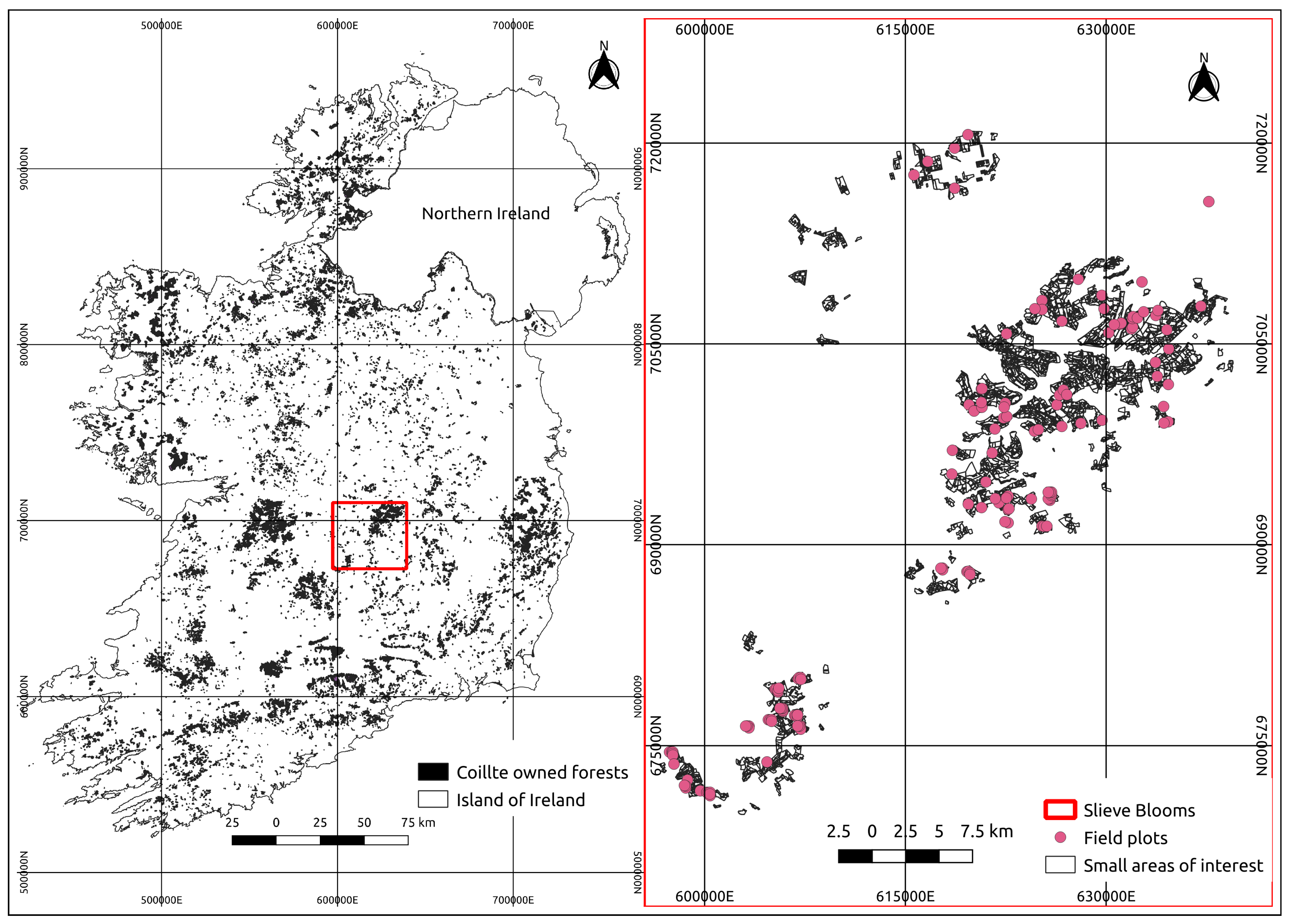
2.1. Study Area

The study area was the forested area managed by Coillte, the State Forestry Board, in the Slieve Blooms mountains which are located across counties Laois and Offaly in the Republic of Ireland (Figure 1). The Slieve Blooms was chosen as the AOI as it has multipurpose forests that provide sustainable timber production and recreational services. The AOI contains approximately 11,800 ha of forested area consisting of 9500 ha of Sitka spruce (Picea sitchensis (Bong.) Carr.) (SS), 1300 ha of Lodgepole pine (Pinus contorta Dougl.) (LP), and 300 ha of Norway spruce (Picea abies (L.) H.Karst) (NS). Other species include European larch (Larix decidua Mill.), Japanese larch (Larix kaempferi (Lamb.) Carr.), and silver birch (Betula pendula, Roth.) along with other broadleaved species. Typically tree species are intimately mixed, planted at a 2 × 2 m spacing to produce a stem density of approximately 2500 stems per hectare. Most forest stands have two thinning interventions, removing approximately one third of the stems in each intervention. The AOI has a mean elevation of 300 m above sea level [24] and contains approximately 50% blanket peat, with a mixture of luvisols, groundwater gleys, and stagnic iron-pan podzols soils [25]. The median age of Sitka spruce is 25 years old with typical rotation periods of spruce in Ireland being 30–35 years old. The percentage breakdown of the AOI by age and yield class (YC) shows approximately 25% of the area is greater than or equal to 25 years old and has a YC greater than or equal to 14 m${}^3$ ha${}^{-1}$ year${}^{-1}$ (

Table 1. Percentage breakdown of the Slieve Blooms mountains spruce forests by age and yield class.

Age	Yield Class ≥ 14 m${}^3$ ha${}^{-1}$ year${}^{-1}$	Yield Class < 14 m${}^3$ ha${}^{-1}$ year${}^{-1}$
≥25 years old	25%	15%
<25 years old	52%	8%

). Yield class is a productivity measure indicating the maximum mean annual increment of cumulative timber volume [26].

2.2. Field Inventory

Field inventory data were collected for the AOI during the summer of 2018 based on stratified random sampling by primary species (SS and LP) and age. The total number of field plots was 136, each of which was geo-located using a Trimble R1 differential global positioning system device with real-time correction (±1 m accuracy). All circular field plots had a radius of 11.28 m on a flat plane and adjusted for slopes greater than 10°. All trees with a DBH greater than 7 cm on a plot were measured with a Haglof digital calipers and transponder. Where a tree was outside the radius by less than 0.1 m using the calipers, which uses a transponder to calculate if a tree is within the radius or not, a tape measure was used for corroboration. The tree was included if the distance measured by the tape measure was within the radius. The associated heights of the minimum, maximum, 25th, 50th, and 75th percentile of measured DBH trees per species were recorded using a Haglof VERTEX IV. The data were then aggregated by plot and species to calculate parameter estimates such as QMDBH (cm), basal area (m² ha⁻¹), stem density (ha⁻¹), and volume (m³ ha⁻¹) (

Table 2. Field inventory measurements.

	Training			Validation
Parameter	Minimum	Maximum	Mean	Minimum	Maximum	Mean
QMDBH (cm)	9	43	20	20	44	28
Basal area (m2 ha−1)	2	108	45	26	74	47
Stems (ha−1)	275	3,250	1498	279	2200	953
Volume (m3 ha−1)	12	1308	412	296	872	535
Age (Years)	10	50	29	27	55	37

). Volume was calculated using the British Forestry Commission stand tariff system [27]. This meant that there would be a value for each of the above parameters for each species per plot. These data were used as training data during the modelling process (Table 2).

Another field inventory dataset collected within the AOI in 2016, 2017, and 2018 was used as validation (Table 2). Prior to clearfelling, stand-level inventory was performed to estimate the standing volume and value. These areas are mature stands with slow growth rates, meaning this inventory should be a good indicator for what will be clearfelled and therefore a valuable validation dataset. To ensure statistically robust comparisons between the estimated values and the validation data, only forests that where the dominant species was SS or NS, greater than or equal to 25 years old, and had a YC greater than or equal to 14 m${}^3$ ha${}^{-1}$ year${}^{-1}$ were used in the modelling process. This subsample represents approximately 25% of the entire AOI. It was chosen to be a representative sample as the error between estimated values and measured values should be minimal due to the slow growth and spacing of thinned mature stands (Table 1). The results from this dataset are expected to be representative of the other 52% of the AOI once they are at least 25 years old, i.e., 52% of the AOI have a YC greater than 12 m${}^3$ ha${}^{-1}$ year${}^{-1}$ but are not yet greater than or equal to 24 years old. This expectation is dependent on the YC remaining above 12 m${}^3$ ha${}^{-1}$ year${}^{-1}$. There are 349 plots in this dataset which were measured using similar methodology as described above with the exceptions being that only the heights of the maximum, minimum, and mean dbh trees per species were measured and the field plot size could be altered based on stocking density present. Although there are 349 plots, these are aggregated to derive median estimates of parameters for a range of areas. Any area with less than ten field plots in it was excluded. Due to the complexity of the methodology and numerous sources of data, a summarised workflow is presented (Figure 2).

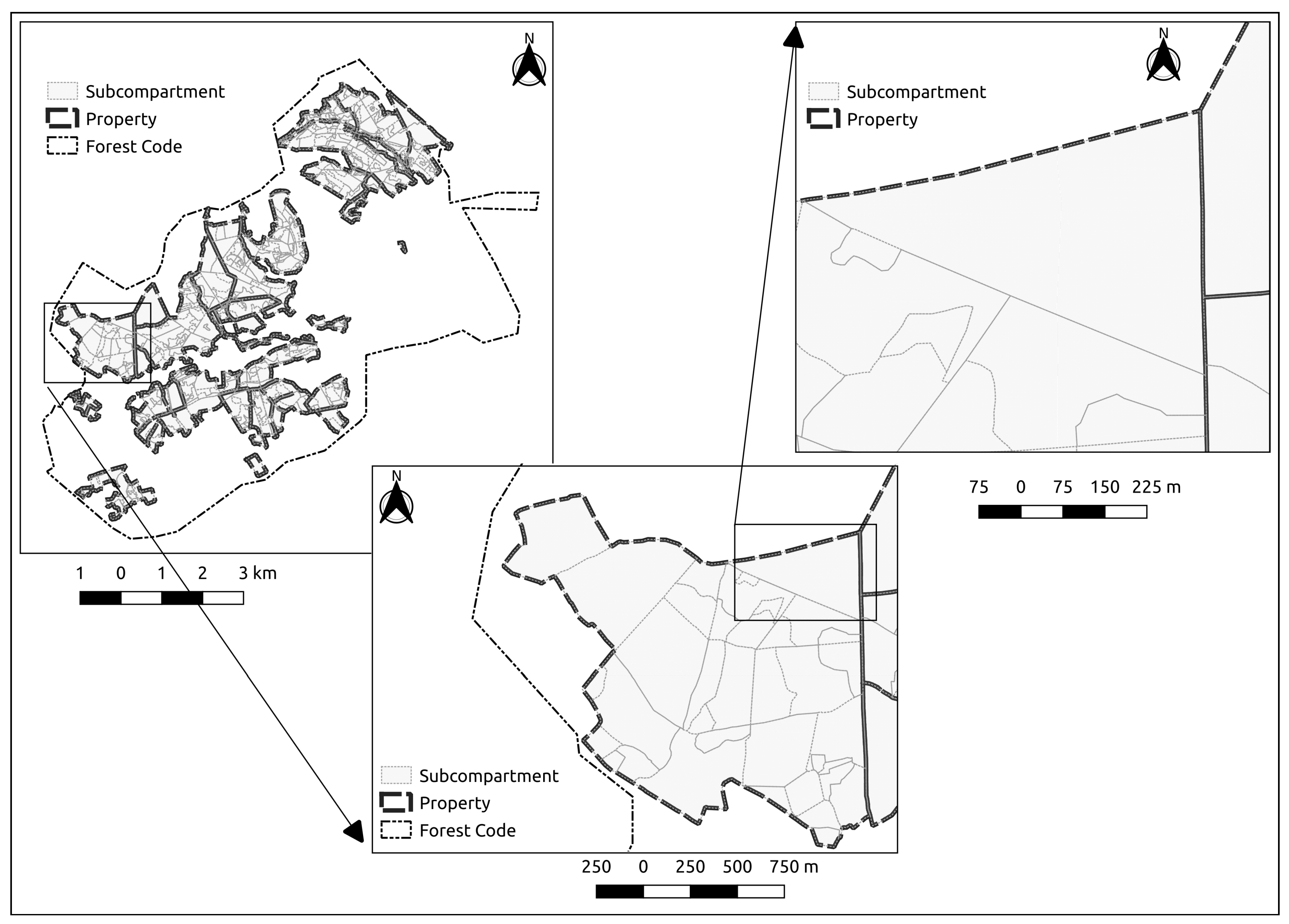
2.3. Spatial Aggregation Layers

Forests can be managed at a variety of spatial scales, the minimum of which, for this study, is a subcompartment (

Table 3. Management scale details for the Slieve Blooms.

Scale	Minimum Area (ha)	Mean Area (ha)	Median Area (ha)	Maximum Area (ha)
Subcompartment	0.5	4.3	2.5	55
Property	2.4	92	47	660
Forest code	42	797	640	2216

). Subcompartments are delineated as polygons according to species, age, and height if available. Neighbouring subcompartments can be aggregated to a larger polygon, called Compartments, and aggregated again to a larger polygon called a Property based on geographical location. Neighbouring Properties can be further aggregated to larger polygons known as Forest codes which are arbitrary codes based on location (Figure 3). These three layers—subcompartment, Property, and Forest Code—were used to create a range of areas to (i) validate the model and (ii) assess the effects of areal size in variance estimation. This was achieved by aggregating the polygons in the subcompartment layer according to polygons in the Property layer and also the Forest Code layer. For example, if there are six subcompartment polygons within two Property polygons, the six measured field plot values are aggregated to two mean measured values, one for each polygon in the Property layer. If these six subcompartment polygons were within one Forest Code polygon, then the six field plot values are aggregated to one mean measured value. It is crucial to note that although the size of the polygons in the subcompartment, Property, and Forest Code layers differ (Table 3), the total size of the area never changed from one layer to another, as only the polygons of the subcompartment within the other layers were used. It was possible to aggregate the areas as such because the species were the same, YC was greater than 14 m${}^3$ ha${}^{-1}$ year${}^{-1}$, and the age profile of these areas were in a similar growth stage, i.e., they were all productive, mature, spruce forests. Herein, the names of the layers will not be mentioned as only the actual size of the area is important. For example, the variance of a polygon 10 ha in size from the subcompartment layer would yield the same variance if it was the only and exact same area in the Property layer.

2.4. Auxiliary Variables

Four sources of auxiliary variables were used, the first of which was lidar. The lidar campaign was flown during July and August of 2018, capturing approximately 11,800 ha of forested area with flight and sensor parameters specified pre-flight (

Table 4. Lidar acquisition details.

Parameter	2018
Sensor	Optech Galaxy T1000
Maximum altitude flown (m)	1200
Speed of plane (knots)	110
Scan angle (degrees off nadir)	14
Flight lines overlap (%)	20
Pulses (per m${}^2$—all returns)	4

). The lidar data was georeferenced using 10 ground control points surveyed using differential GPS. The lidar dataset was processed using the Sorted Pulse Data library (SPDlib) which is a free and open source command line lidar processing software [28]. The processing steps included

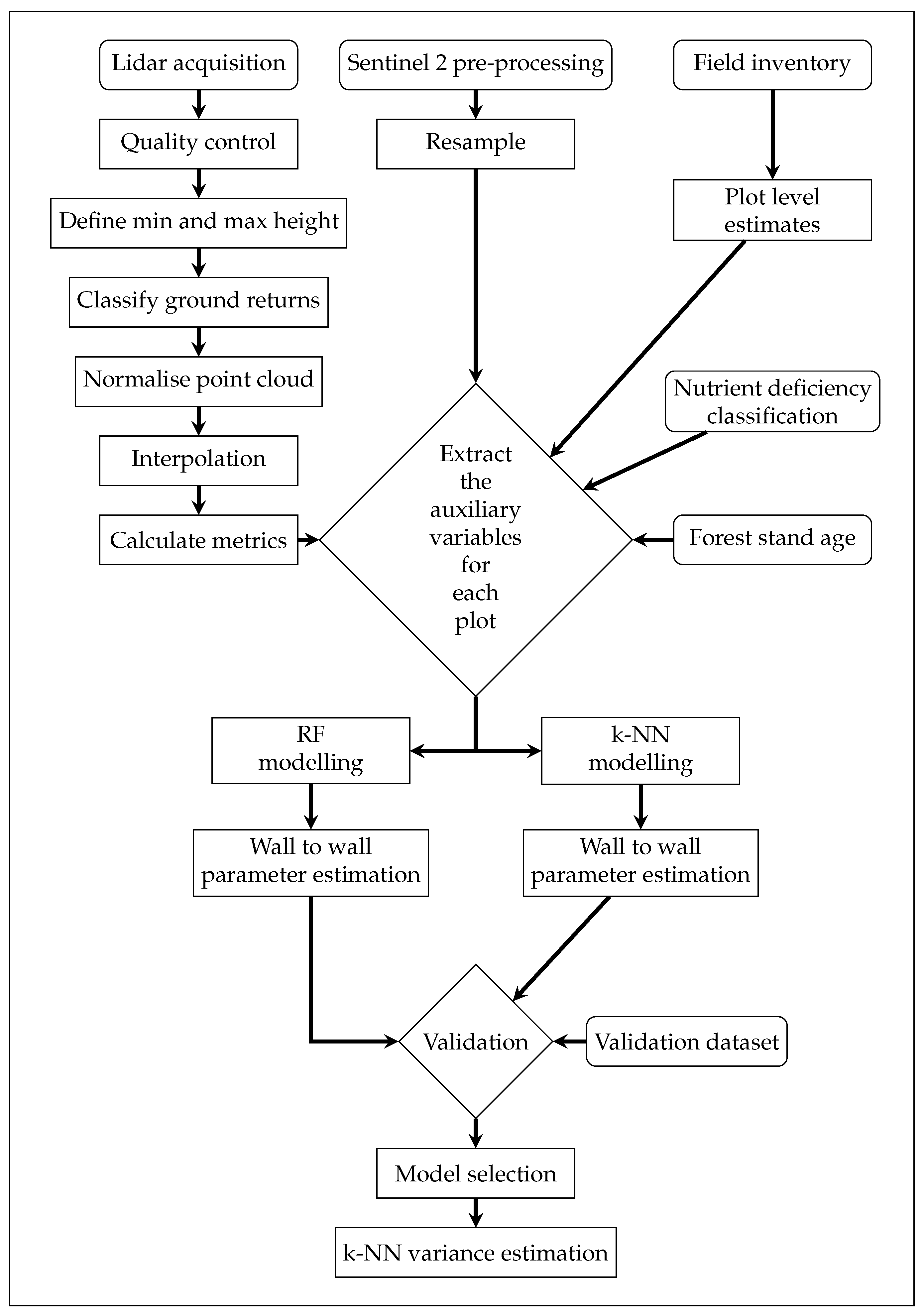
• a quality control check to ensure the point cloud had no anomalies or issues;
• removing noise by defining a local and global minimum and maximum height threshold;
• classifying ground returns using a progressive morphology filter [29] and a multi-scale curvature algorithm [30];
• point cloud normalisation;
• interpolating surfaces to create a canopy height model (CHM), digital terrain model (DTM), and digital surface model (DSM); and
• calculating metrics.

A natural neighbour algorithm was implemented in order to create the CHM, DTM, and DSM products at 1 m resolution, and a range of metrics were calculated (

Table 5. Auxiliary variables used during modelling.

Lidar Metric	Return	Details
Height	All returns that were not ground	Minimum, maximum, mean, median, mode, dominant, 10, 20, 30, 40, 50, 60, 70, 80, 90, 100 percentile heights, standard deviation for all height percentiles, kurtosis, variance, skewness, sum.
Height	All	Minimum, maximum, mean, median, mode, dominant, standard deviation, kurtosis, variance, skewness, sum.
Height	First	Minimum, maximum, mean, median, mode, dominant, standard deviation, kurtosis, variance, skewness, sum.
Height	Last	Minimum, maximum, mean, median, mode, dominant, standard deviation, kurtosis, variance, skewness, sum.
Density	All returns that were not ground	Between 2 m–40 m, 2.5 m–5 m, 5 m–10 m, 10 m–15 m, 15 m–20 m, 20 m–25 m, 25 m–30 m, 30 m–40 m.
Canopy cover percent	All returns that were not ground	Between 2.5 m–5 m, 5 m–7.5 m, 7.5 m–10 m, 10 m–12.5 m, 12.5 m–15 m, 15 m–17.5 m, 17.5 m–20 m, 20 m–22.5 m, 22.5 m–25 m, 25 m–27.5 m, 27.5 m–30 m, 30 m–40 m.
Amplitude	All returns that were not ground	Sum, mean, median, max, standard deviation, variance, percentile 10–100
Height density [10]	All	95th Percentile between 2 m and 40 m height.
Sentinel 2		Bands 1, 2, 3, 4, 5, 6, 7, 8, 9, 10
Sentinel 2		Nutrient deficiency classification
Internal database		Age of forest

variables in bold were removed during modelling as they provided less than 1% increase in MSE.

) based on a 20 × 20 m grid cell to ensure equivalence with the field plot area. The second source was cloud-free multi-spectral satellite imagery from the Sentinel 2 mission, acquired during the Spring and Summer months of 2018. The images were atmospherically corrected and all pixels were resampled to 20 × 20 m using ARCSI [31] and a nearest neighbour algorithm. The third source of auxiliary variables was a multi-spectral derived nutrient deficiency classification for the AOI [32]. The final source of auxiliary variables was the age of the forest stands from Coillte’s spatial database. In total there was 97 auxiliary variables used, 85 lidar metrics, 10 Sentinel 2 bands, a Sentinel 2 nutrient deficiency classification, and the age of the forests. All of the auxiliary data were georeferenced to Irish Transverse Mercator (EPSG:2157) and quality control of the spatial data suggested a high spatial accuracy between layers.

2.5. Parameter Estimation

This study utilised the well-documented area-based approach (ABA) [6,7] for modelling ground data and auxiliary variables to produce parameter estimates per grid cell. Two machine learning algorithms were employed in this study—Random Forest (RF) and a weighted k-NN—in the statistical programming language R [33]. The RF modelling included removal of auxiliary variables according to the variable importance plot [34] assessed by the percent increase in mean squared error (MSE), where if the variable had an increase of less than one percent, it was removed. This removed 10 of the 97 auxiliary variables, mainly the Sentinel 2 bands. From the remaining variables, the most important were max height, standard deviation of heights, and the 80th percentile height for all returns that were not classified as ground. The modelling also included a grid search for the best mtry and ntree, as determined by the root MSE (RMSE). The Euclidean distance was used as the distance metric for the grid search and validated using a 10 repeat cross-validation. The weighted k-NN modelling, using the kknn package [35], trialled all available kernels using the Minkowski distance metric and assessed the best using a leave one out cross validation. The range of k values tested was from 2 to 10, as a meta-analysis of k-NN studies concluded that the most frequently used values of k in remote sensing applications applied to forestry are within this range [36]. The parameter estimates were compared by calculating the RMSE, RMSE%, R${}^2$, and bias.

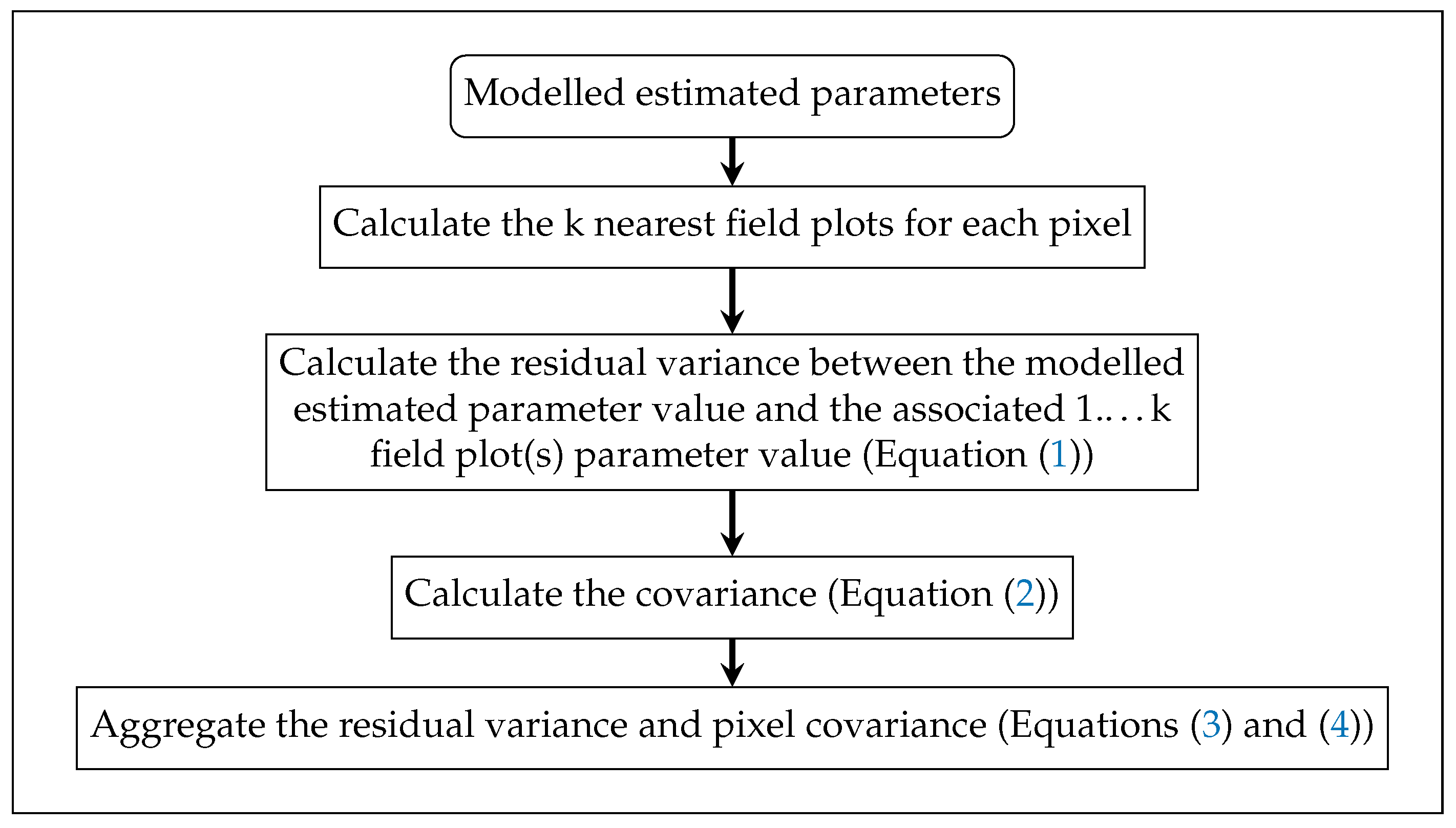
2.6. Variance Estimation

Estimation of variance for the parameter estimates was carried out using a methodology developed in [13], further explained in the initial description in [23], and summarised below (Figure 4). This methodology can incorporate spatial correlation but is not included in the description below as no spatial correlation was present using the semi-variogram methodology [13]. This variance estimation technique is derived by first equating the estimated value or prediction, ${\tilde{y}}_i$ to both the mean, ${\mu }_i$ and realisation, $y_i$ of values in a regression context [13,37]. The next step of the methodology is to calculate which k number of measured plots are nearest in the covariate space according to the auxiliary variables for each pixel. Once this is complete, the residual variance between the measured and estimated value for the above k plots for each pixel is calculated using

$${\hat{\sigma }}_i^2=\frac{{\displaystyle \sum _{j=1}^k}{(y_j^i-{\hat{\mu }}_i)}^2}{k-1}$$

(1)

where {$y_j^i,j=1,2,\dots ,k$} is the set of response variable observations for the k reference set elements, or pixels in this example, that are nearest to the ith pixel in feature space, ${\hat{\mu }}_i$ is the mean for the ith pixel, and k is the number of nearest neighbours.

Following that, the covariance between the ith pixel estimate and jth pixel estimate for all pixels is calculated within the defined small area (Equation (2)).

$$C\hat{o}v({\hat{\mu }}_i,{\hat{\mu }}_j)\approx \frac{m_{i_j}{\hat{\sigma }}_i{\hat{\sigma }}_j}{k^2}$$

(2)

where $m_{i_j}$ is the number of field plots that are common to both the ith and jth pixels and ${\hat{\sigma }}_i$${\hat{\sigma }}_j$ can be estimated by substituting ${\hat{\sigma }}_i$ from (1).

Finally, calculate the variance for the small area by aggregating the residual variance and pixel covariance estimates by substituting (2) and (3) into (4).

$$V\hat{a}r\left({\hat{\mu }}_i\right)\approx \frac{{\hat{\sigma }}_i^2}{k}$$

(3)

$$Var\left(\hat{\mu }\right)=\frac{1}{N^2}\left[\sum _{i=1}^{N}Var\left({\widehat{\mu }}_i\right)+2\sum _i^N\sum _{<j}^{N}Cov({\widehat{\mu }}_i,{\widehat{\mu }}_j)\right]$$

(4)

where N is the number of pixels.

In [13], the exact variance was not calculated for each AOI, instead, after calculating the exact variance for three AOIs, it was concluded that the variance would not change significantly after approximately 15% of the pixels had been processed. This is due to the large size of the AOIs in [13]. In this investigation, the exact variance was calculated for each AOI, as they are much smaller. k values from 2 to 7 were tested and the variance was compared using the relative standard deviation (RSD) which is expressed as twice the square root of the variance as a percentage of the mean.

$$RSD=\frac{2\sqrt{Var\left(\hat{\mu }\right)}}{\hat{\mu }}100$$

(5)

using

$$\hat{\mu }=\frac{1}{N}\sum _{i=1}^N{\hat{\mu }}_i=\frac{1}{N}\sum _{i=1}^N{\tilde{y}}_i$$

(6)

3. Results

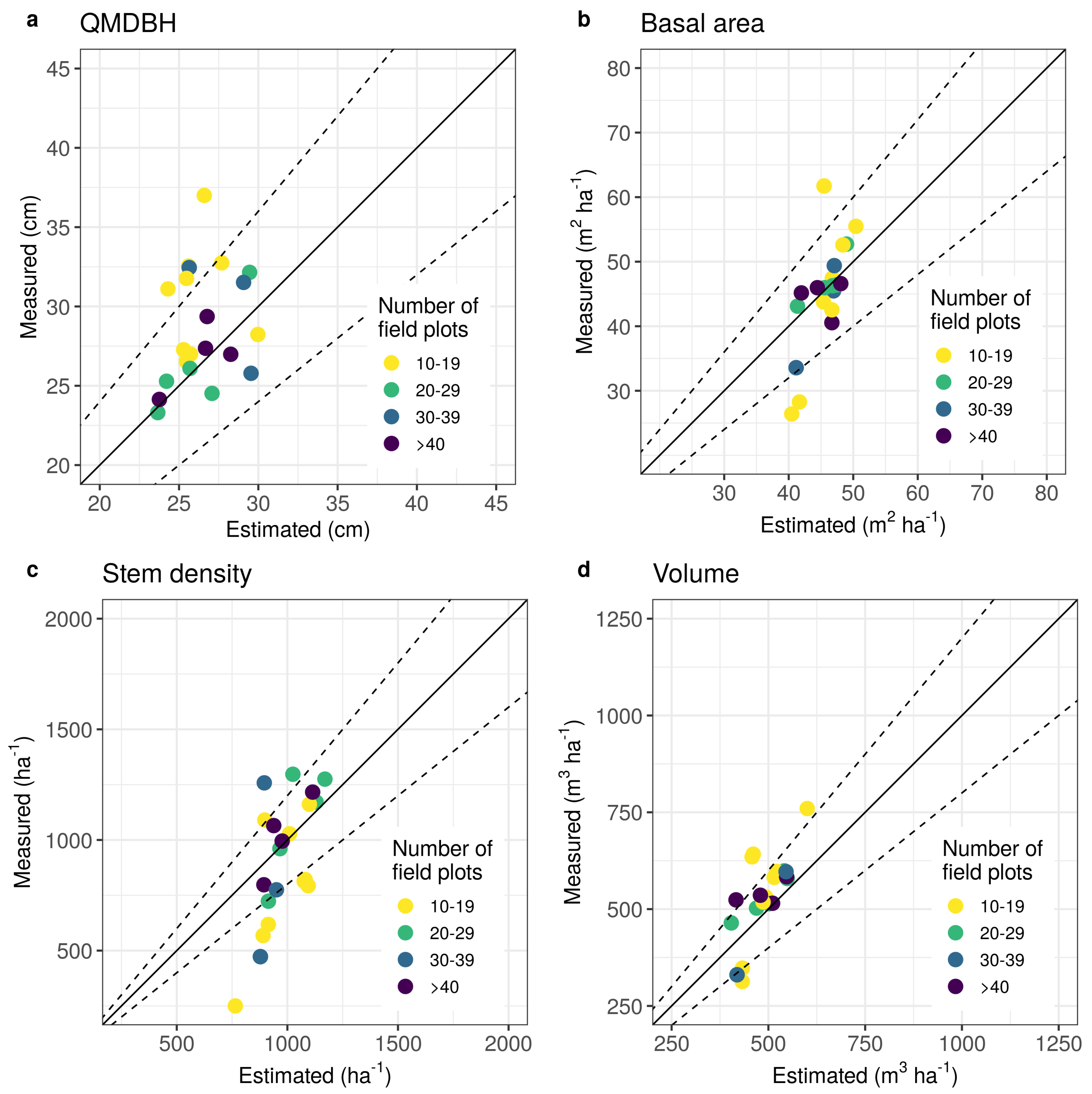
3.1. Parameter Estimation

The RMSE, RMSE%, R${}^2$, and standardised bias results for modelling QMDBH, basal area, stem density, and volume using a RF and weighted k-NN model with all field plots and just majority Spruce field plots are presented (

Table 6. Random Forest modelling results for all field plots (AF) and only using majority Spruce field plots (Spruce).

Parameter	AF				Spruce
	RMSE	RMSE (%)	R${}^2$	Bias	RMSE	RMSE (%)	R${}^2$	Bias
QMDBH (cm)	3.95	19	0.70	0.0303	4.21	19	0.69	0.1179
Basal area (m${}^2$ ha−1)	9.95	22	0.67	0.0778	10.49	21	0.61	0.0775
Stems (ha−1)	420	28	0.62	1	409	27	0.69	8
Volume (m${}^3$ ha−1)	110	26	0.77	2	111	23	0.75	4

and

Table 7. Weighted k-NN modelling results for all field plots (AF) and only using majority Spruce field plots (Spruce).

Parameter	AF				Spruce
	RMSE	RMSE (%)	R${}^2$	Bias	RMSE	RMSE (%)	R${}^2$	Bias
QMDBH (cm)	4.83	24	0.58	0.1141	5.40	26	0.54	0.1111
Basal area (m${}^2$ ha−1)	10.52	23	0.64	0.1380	11.23	23	0.57	0.4066
Stems (ha−1)	461	31	0.56	5	465	30	0.62	45
Volume (m${}^3$ ha−1)	121	29	0.72	3	132	28	0.65	7

). RF modelling for QMDBH using all field plots resulted in a 3.95 cm RMSE, equivalent to 19%, with an R${}^2$ value of 0.7. The RMSE value increased to 4.83 cm when using the weighted k-NN model. The QMDBH RMSE was 4.21 cm with a similar 19% RMSE% and R${}^2$ value of 0.69 when using majority Spruce field plots. The RMSE value increased to 5.33 cm when using the weighted k-NN model. For the other parameters, the RF RMSE values are all smaller compared to the weighted k-NN model while the R${}^2$ values are all greater. All RMSE values are based on pixel comparisons using a repeated cross-validation methodology. The mtry and ntree values for the RF modelling were 9 and 500, respectively.

The mean parameter estimates versus mean measured results are shown for each parameter coloured by the number of field plots in each point (Figure 5). The mean measured values are calculated for areas which contain at least ten field plots which means there are 22 data points in this figure. For areas with 10–19 field plots, some underestimation is present for QMDBH (a) while both under and over estimation is present for basal area (b). Approximately half of the data points for stem density lie outside the 20% error lines. Overall, as the number of field plots increases the data point tends to be within the 20% error lines for QMDBH, basal area, and volume.

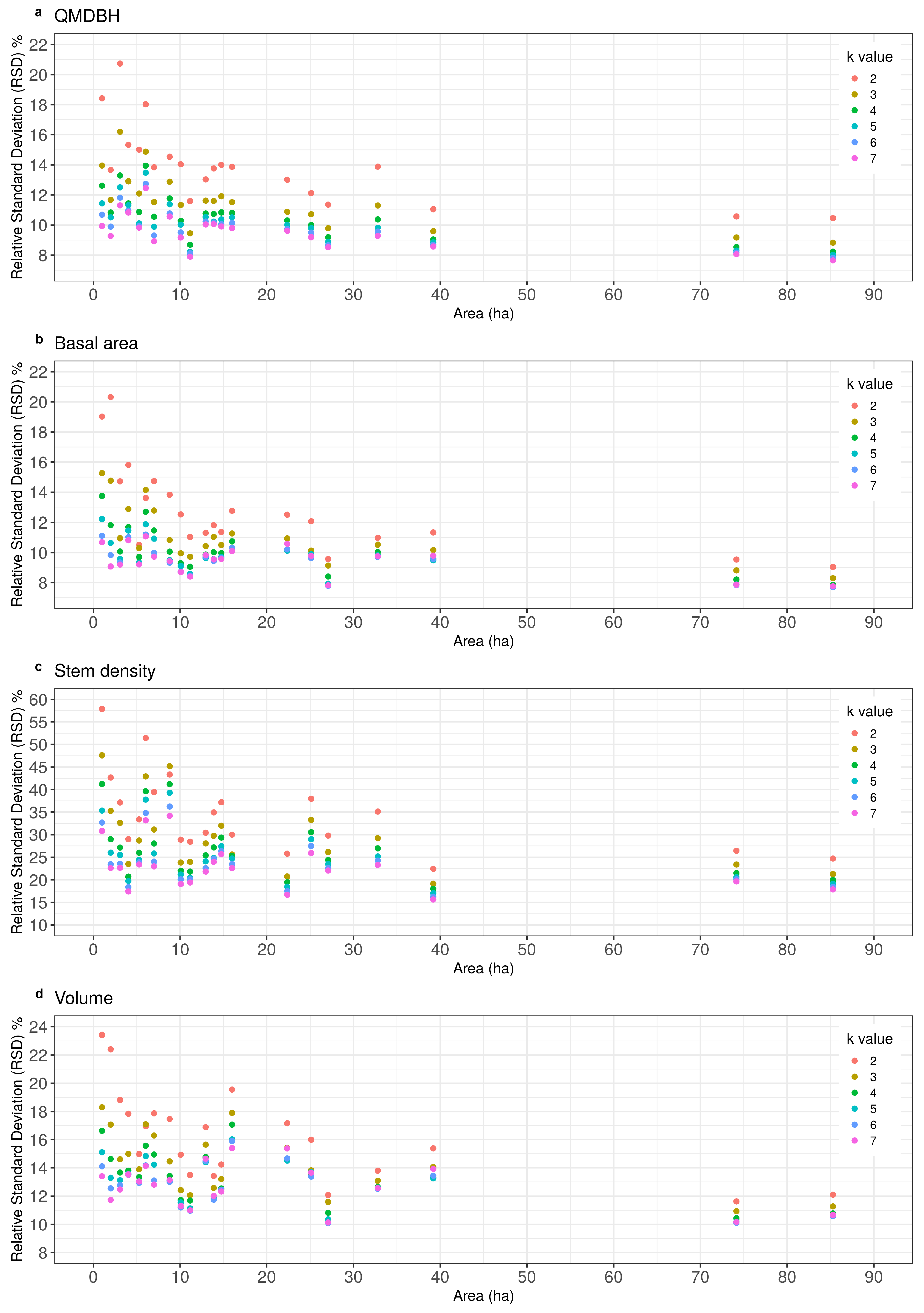
3.2. Variance Estimation

The RSD for all parameters at a range of areas are presented (Figure 6a–d). The results for all parameters have the same trend, which is, for any area, as the k value increases, the RSD decreases. When using a k value of 2, the RSD is greater for areas less than 10–15 ha than it is for areas greater than 15 ha. The difference in RSD from using a low k value, such as 2, compared to a larger k value, such as 6, is greater for areas less than 10–15 ha compared to areas greater than 15 ha.

4. Discussion

4.1. Parameter Estimation

In this study, we estimated QMDBH, basal area, stem density, and volume using two different machine learning algorithms: RF and k-NN. Using the optimum model of a low RMSE and a high R${}^2$ value, the RF model was used to estimate the variance of each parameter. The variance estimation uses a k-NN estimation technique, which is separate from the modelling process. We investigated how k values between 2 and 7 and the size of the small area affect the variance.

The QMDBH results can be difficult to place in an international context as few studies have modelled QMDBH for the same species investigated here. However, a comparison with other studies is still useful as our results are at the upper thresholds of the range of values reported in the literature. An investigation of plantation conifers in Ontario, Canada using ALS resulted in an RMSE of 11% with an R${}^2$ value of 0.83 [38]. Another ALS study of mixed-conifer stands in northern Idaho, United States of America, obtained an R${}^2$ value of 0.61 [39]. Furthermore, QMDBH estimates using ALS in Sweden for Norway spruce (Picea abies) and Scots pine (Pinus sylvestris) plantation crops achieved an RMSE of 8.9% [40]. Although the reported RMSE% is comparably high to these studies, the differences in the environment and species cannot be overstated as forests are highly fragmented in Ireland with a large variation in age and growth rates across the country. Nonetheless, the R${}^2$ value of 0.70 from our results show that the model has captured the majority of variance for QMDBH.

Modelling basal area is more common in the literature. For example, stand estimates for areas dominated mainly by western red cedar (Thuja plicata) and western hemlock (Tsuga heterophylla) using ALS and Landsat time series data showed an RMSE of 18% and an R${}^2$ value of 0.75 [41]. Pine (Pinus radiata) estimates in New Zealand using ALS resulted in an RMSE of 4.5% and an R${}^2$ value of 0.69 [42]. Basal area estimates in Sweden for Norway spruce (Picea abies) and Scots pine (Pinus sylvestris) using ALS results in an RMSE of 15% and RMSE 10% respectively [43]. Standard deviations between 14.1 and 23.0% were obtained for Norway spruce (Picea abies) and Scots pine (Pinus sylvestris) in Norway [11]. Comparing our results to the above studies, the modelling results are on the upper scale of what has been previously reported.

The RF modelling RMSE for stem density is 420 ha${}^{-1}$ (28%) with an R${}^2$ value of 0.62. Although the R${}^2$ value can be considered a reasonable value, the RMSE and RMSE% are too large to be considered useful in a commercial setting in Ireland. As a result, the linking model has not effectively captured the stem density on the ground. Stem density has been problematic for other studies due to the sub-dominant tree stems that do not reach the upper canopy likely being missed in the lidar returns [38,44].

The volume results show a good comparison with other international studies such as that in [45], the authors of which used national forest inventory data from Italy to model volume using satellite imagery, microwave sensor data, a ALS derived CHM, in addition to meteorological data. Their investigation resulted in an R${}^2$ value of 0.69 and an RMSE of 37.2% using an independent dataset. Other investigations for estimating volume attained an RMSE of 27% and an R${}^2$ value of 0.67 for western red cedar (Thuja plicata) [41]; 19% and 11% at two previously mentioned sites in Sweden for Norway spruce (Picea abies) and Scots pine (Pinus sylvestris) [43], respectively; and an R${}^2$ value of 0.46 for a mix of spruce and pine [9]. Volume estimates for Norway spruce (Picea abies) were also modelled at a site in Freiburg, Germany, using low-density ALS [15]. They obtained root mean squared distance of 99% for their spruce volume model due to the complexity of the modelled area including a diverse range of species. Calculation of root mean square distance is identical to RMSE. They also modelled a combination of coniferous species together, which yielded better results, an RMSE of 44.23% using a k-NN modelling approach. Similar to the basal area results, the modelling results are on the upper scale of what has been previously reported. Based on the results from the RMSE, RMSE%, R${}^2$, and bias (Table 6 and Table 7), the RF model estimates were used in the variance estimation.

A graph of the mean measured versus mean estimated parameter values for a number of areas shows that the model is able to produce estimates consistent with the measured data (Figure 5a–d). There are a number of data points that have been underestimated QMDBH (a) and volume (d), and also both under and over estimation basal area (b), however the vast majority of points for QMDBH, basal area, and volume are all within the 20% error lines. This graph also illustrates that as the number of field plots within an area increases, the more likely it is to be within the 20% error lines for all parameter except stem density. This result is not unusual as the mean measured value is being compared to the mean estimated value for an area and so the areas are better estimated with more field plots included. The lack of fit with the stem density is due to the limitations of the linking model to capture sub-dominant stems which is also evident from the results in Table 6. Nonetheless, the results for QMDBH, basal area, and volume adds further weight to Table 6 to prove that the model has been able to accurately capture these parameters on the ground. As the variance estimation relies on the linking model being able to describe an area, this result will allow for confidence in the variance estimation results.

4.2. Variance Estimation

There is ample literature regarding the estimation of forest parameters using model-based inference [46,47,48,49] and numerous which investigate increasing k values with decreasing error estimates [13,15,23,36]. However, few studies have examined the effects of k and the size of an area with respect to variance estimation of multiple pixel AOIs, making this study a timely addition to the literature. The main benefit of utilising this variance estimation technique is that a variance estimate can be obtained when aggregating multiple pixels, which is not widely reported in the literature. Consequently, the effects of k and the size of the AOI have not been investigated in depth in relation to variance estimation of multiple pixel AOIs.

Note that the variance estimation relies on the capability of the model to accurately capture the AOI, and so if the model does not capture the AOI, the variance estimation will not be useful. This can be seen in Figure 6c where the variance estimation of stem density is shown. The linking model in the parameter estimation showed poor correlation with validation data and as a result was deemed to not have effectively captured the stem density. The RSD values show this where the majority of areas between 10–15 ha have RSD values of 20–40%, which is too large to be considered useful in an operational setting. The RSD values improve when investigating larger areas, however the underlying model is still the same and so does not represent a model better able to represent the study area. This is why particular attention should be placed on training and validating the underlying linking model.

The RSD for all parameters at a range of areal sizes show that as the k value increases, the RSD decreases (Figure 6a–d). This result is not surprising as the k value is in the denominator of Equations (1)–(3) in the variance estimation. Although the numerator would increase due to the addition of another value for each equation as the k value increases, the magnitude of the denominator is far more influential and so, as it increases, the magnitude of Equations (1)–(3) decreases. This decrease is far more pronounced for areas less than 10–15 ha in size. Areas greater than this are less affected by the change in the value of k due to the greater value of N, the number of pixels, in the denominator of Equation (4). Therefore, the dominant variable in estimating variance for areas less than 15 ha using this methodology is the value of k.

This does not mean any one AOI will have a lower RSD than any other AOI, just based on the fact that it is a larger area, as different AOIs will have different characteristics and therefore different variances. This is shown in the QMDBH graph for the AOI at approximately 4 ha, in the basal area graph for the AOI at approximately 5.2 ha, and in the volume graph for the AOI at 39 ha (Figure 6a,b,d), where AOI’s with a greater area did not always obtain smaller RSD. Similar results using a different variance estimation technique for forest parameters have also resulted in decreasing RSD with increasing area size, however, all of these studies have considerably larger ’small’ areas than the areas presented within this study [50,51,52]. Studies that investigated similar sized small areas showed consistent trends of decreasing RSD with increasing AOI size for volume [15,53]. A comparison of RSD between studies is not applicable as different AOI’s with different species and stocking are not comparable. Nonetheless, the trend of increasing area sizes with reducing variance estimates is consistent. This study therefore shows the applicability of the k-NN variance estimation technique for a range of study areas and its utility in estimating variance for multiple pixel AOI. Forest managers utilising this technique will be able to make better management decisions as the addition of the associated parameter estimate variance gives an enhanced description, and therefore understanding, of the AOI.

5. Conclusions

The conclusions from this investigation are threefold: First, the results from implementing this methodology show that the parameter estimation of areas less than 10–15 ha in size yielded greater uncertainty than areas greater than 15 ha. Second, the results from the k value analysis illustrated that as the k value increases, the variance, as described by the RSD, decreases, and that this decrease is more prominent for smaller areas (10–15 ha). Finally, as area increases, the variance decreases for any value of k albeit, not indefinitely. These results illustrate the applicability of the technique to provide precise variance estimates for small areas of multiple pixel AOIs. This work can be used as a reference guide for researchers, forest managers, and inventory assessors when estimating variance of forest attributes as it will allow for variance estimates of multiple pixel AOIs and also how the variance is affected by the value of k and the size of the AOI. This work also demonstrates the applicability of using a random forest model with this k-NN variance estimation technique in another operational setting.

References

1. Smith, T.M.F. The Foundations of Survey Sampling: A Review. J. R. Stat. Soc. Ser. A (Gen.) 1976, 139, 183. [Google Scholar] [CrossRef]
2. Rao, J.N.K. Small Area Estimation, 1st ed.; Wiley: Hoboken, NJ, USA, 2003; pp. 1–3. [Google Scholar]
3. Kangas, A.; Maltamo, M. Forest Inventory: Methodology and Applications; Springer: Dordrecht, The Netherlands, 2006; Volume 10, pp. 39–51. [Google Scholar]
4. Gregoire, T.G. Design-based and model-based inference in survey sampling: Appreciating the difference. Can. J. For. Res. 1998, 28, 1429–1447. [Google Scholar] [CrossRef]
5. Mandallaz, D. A Unified Approach to Sampling Theory for Forest Inventory Basedon Infinite Population and Superpopulation Models. Ph.D. Thesis, Swiss Federal Institute of Technology (ETH), Zurich, Switzerland, 1991. [Google Scholar]
6. Næsset, E. Determination of mean tree height of forest stands using airborne laser scanner data. ISPRS J. Photogramm. Remote Sens. 1997, 52, 49–56. [Google Scholar] [CrossRef]
7. Maltamo, M.; Næsset, E.; Vauhkonen, J. Forestry Applications of Airborne Laser Scanning. In Managing Forest Ecosystems, 1st ed.; Springer: Dordrecht, The Netherlands, 2014; Volume 27, Chapter 11; p. 462. [Google Scholar] [CrossRef]
8. Tomppo, E. Satellite image-based national forest inventory of Finland. In Proceedings of the Symposium on Global and Environmental Monitoring, Techniques and Impacts, Victoria, BC, Canada, 17–21 September 1990; pp. 419–424. [Google Scholar]
9. Næsset, E. Estimating timber volume of forest stands using airborne laser scanner data. Remote Sens. Environ. 1997, 61, 246–253. [Google Scholar] [CrossRef]
10. Næsset, E.; Bjerknes, K.O. Estimating tree heights and number of stems in young forest stands using airborne laser scanner data. Remote Sens. Environ. 2001, 78, 328–340. [Google Scholar] [CrossRef]
11. Næsset, E. Predicting forest stand characteristics with airborne scanning laser using a practical two-stage procedure and field data. Remote Sens. Environ. 2002, 80, 88–99. [Google Scholar] [CrossRef]
12. Breidenbach, J.; Astrup, R. Small area estimation of forest attributes in the Norwegian National Forest Inventory. Eur. J. For. Res. 2012, 131, 1255–1267. [Google Scholar] [CrossRef]
13. McRoberts, R.E.; Tomppo, E.O.; Finley, A.O.; Heikkinen, J. Estimating areal means and variances of forest attributes using the k-Nearest Neighbors technique and satellite imagery. Remote Sens. Environ. 2007, 111, 466–480. [Google Scholar] [CrossRef]
14. McRoberts, R.E.; Næsset, E.; Gobakken, T. Inference for lidar-assisted estimation of forest growing stock volume. Remote Sens. Environ. 2013, 128, 268–275. [Google Scholar] [CrossRef]
15. Breidenbach, J.; Nothdurft, A.; Kändler, G. Comparison of nearest neighbour approaches for small area estimation of tree species-specific forest inventory attributes in central Europe using airborne laser scanner data. Eur. J. For. Res. 2010, 129, 833–846. [Google Scholar] [CrossRef]
16. Chirici, G.; McRoberts, R.E.; Fattorini, L.; Mura, M.; Marchetti, M. Comparing echo-based and canopy height model-based metrics for enhancing estimation of forest aboveground biomass in a model-assisted framework. Remote Sens. Environ. 2016, 174, 1–9. [Google Scholar] [CrossRef]
17. McRoberts, R.E.; Chen, Q.; Walters, B.F. Multivariate inference for forest inventories using auxiliary airborne laser scanning data. For. Ecol. Manag. 2017, 401, 295–303. [Google Scholar] [CrossRef]
18. McInerney, D.; Barrett, F.; McRoberts, R.E.; Tomppo, E. Enhancing the Irish NFI using k-Nearest Neighbors and a genetic algorithim. Can. J. For. Res. 2018, 99, 1482–1494. [Google Scholar] [CrossRef] [Green Version]
19. Kangas, A. Small-area estimates using model-based methods. Can. J. For. Res. 1996, 26, 758–766. [Google Scholar] [CrossRef]
20. McRoberts, R.E. A model-based approach to estimating forest area. Remote Sens. Environ. 2006, 103, 56–66. [Google Scholar] [CrossRef]
21. McInerney, D.; Nieuwenhuis, M. A comparative analysis of kNN and decision tree methods for the Irish National Forest Inventory. Int. J. Remote Sens. 2009, 30, 4937–4955. [Google Scholar] [CrossRef]
22. Roberts, O.; Bunting, P.; Hardy, A.; McInerney, D. Sensitivity analysis of the DART model for forest mensuration with airborne laser scanning. Remote Sens. 2020, 12, 247. [Google Scholar] [CrossRef] [Green Version]
23. McRoberts, R.E. Estimating forest attribute parameters for small areas using nearest neighbors techniques. For. Ecol. Manag. 2012, 272, 3–12. [Google Scholar] [CrossRef]
24. EU-DEM. Copernicus Land Monitoring Service; European Environment Agency: Copenhagen, Denmark, 2017. [Google Scholar]
25. Teagasc. Nutrient Deficiencies in Forest Crops; Technical Report 14; Teagasc: Wexford, Ireland, 2007. [Google Scholar]
26. Forest Research. How Forest Yield Works; Forest Research: London, UK, 2020. [Google Scholar]
27. Matthews, R.; Mackie, E. Forest Mensuration: A Handbook for Practitioners; Forestry Comission: Bristol, UK, 2006. [Google Scholar]
28. Bunting, P.; Armston, J.; Lucas, R.M.; Clewley, D. Sorted pulse data (SPD) library. Part I: A generic file format for LiDAR data from pulsed laser systems in terrestrial environments. Comput. Geosci. 2013, 56, 197–206. [Google Scholar] [CrossRef]
29. Zhang, K.; Chen, S.C.; Whitman, D.; Shyu, M.L.; Yan, J.; Zhang, C. A progressive morphological filter for removing nonground measurements from airborne LIDAR data. IEEE Trans. Geosci. Remote Sens. 2003, 41, 872–882. [Google Scholar] [CrossRef] [Green Version]
30. Evans, J.S.; Hudak, A.T. A multiscale curvature algorithm for classifying discrete return LiDAR in forested environments. IEEE Trans. Geosci. Remote Sens. 2007, 45, 1029–1038. [Google Scholar] [CrossRef]
31. Bunting, P.; Clewley, D.; Lucas, R.M.; Gillingham, S. The Remote Sensing and GIS Software Library (RSGISLib). Comput. Geosci. 2014, 62, 216–226. [Google Scholar] [CrossRef]
32. Walshe, D.; McInerney, D.; Kerchove, R.V.D.; Goyens, C.; Balaji, P.; Byrne, K.A.; Forest, C. Detecting nutrient deficiency in spruce forests using multispectral satellite imagery. Int. J. Appl. Earth Obs. Geoinf. 2020, 86, 101975. [Google Scholar] [CrossRef]
33. R Core Team. R: A Language and Environment for Statistical Computing; R Core Team: Vienna, Austria, 2020. [Google Scholar]
34. Liaw, A.; Wiener, M. Classification and Regression by randomForest. R News 2002, 2, 18–22. [Google Scholar]
35. Schliep, K.; Hechenbichler, K. kknn: Weighted k-Nearest Neighbors; Ludwig-Maximilians University Munich: Munich, Germany, 2016. [Google Scholar]
36. Chirici, G.; Mura, M.; McInerney, D.; Py, N.; Tomppo, E.O.; Waser, L.T.; Travaglini, D.; McRoberts, R.E. A meta-analysis and review of the literature on the k-Nearest Neighbors technique for forestry applications that use remotely sensed data. Remote Sens. Environ. 2016, 176, 282–294. [Google Scholar] [CrossRef]
37. Draper, N.R.; Smith, H. Applied Regression Analysis, 3rd ed.; Wiley: New York, NY, USA, 1998; pp. 28–29. [Google Scholar]
38. Woods, M.; Lim, K.; Treitz, P. Predicting forest stand variables from LiDAR data in the Great Lakes - St. Lawrence forest of Ontario. For. Chron. 2008, 84, 827–839. [Google Scholar] [CrossRef] [Green Version]
39. Rooker Jensen, J.L.; Humes, K.S.; Conner, T.; Williams, C.J.; DeGroot, J. Estimation of biophysical characteristics for highly variable mixed-conifer stands using small-footprint lidar. Can. J. For. Res. 2006, 36, 1129–1138. [Google Scholar] [CrossRef]
40. Holmgren, J.; Jonsson, T. Large scale airborne laser scanning of forest resources in Sweden. Int. Arch. Photogramm. Remote Sens. Spat. Inf. Sci. 2004, 36, 157–160. [Google Scholar]
41. Bolton, D.K.; White, J.C.; Wulder, M.A.; Coops, N.C.; Hermosilla, T.; Yuan, X. Updating stand-level forest inventories using airborne laser scanning and Landsat time series data. Int. J. Appl. Earth Obs. Geoinf. 2018, 66, 174–183. [Google Scholar] [CrossRef]
42. Dash, J.P.; Marshall, H.M.; Rawley, B. Methods for estimating multivariate stand yields and errors using k-NN and aerial laser scanning. Forestry 2015, 88, 237–247. [Google Scholar] [CrossRef]
43. Holmgren, J. Prediction of tree height, basal area and stem volume in forest stands using airborne laser scanning Prediction of Tree Height, Basal Area and Stem Volume in Forest. Scand. J. For. Res. 2006, 19, 543–553. [Google Scholar] [CrossRef]
44. Maltamo, M.; Eerikäinen, K.; Pitkänen, J.; Hyyppä, J.; Vehmas, M. Estimation of timber volume and stem density based on scanning laser altimetry and expected tree size distribution functions. Remote Sens. Environ. 2004, 90, 319–330. [Google Scholar] [CrossRef]
45. Chirici, G.; Giannetti, F.; McRoberts, R.E.; Travaglini, D.; Pecchi, M.; Maselli, F.; Chiesi, M.; Corona, P. Wall-to-wall spatial prediction of growing stock volume based on Italian National Forest Inventory plots and remotely sensed data. Int. J. Appl. Earth Obs. Geoinf. 2020, 84, 101959. [Google Scholar] [CrossRef]
46. Puliti, S.; Ørka, H.O.; Gobakken, T.; Næsset, E. Inventory of small forest areas using an unmanned aerial system. Remote Sens. 2015, 7, 9632–9654. [Google Scholar] [CrossRef] [Green Version]
47. Frank, B.; Mauro, F.; Temesgen, H. Model-based estimation of forest inventory attributes using lidar: A comparison of the area-based and semi-individual tree crown approaches. Remote Sens. 2020, 12, 2525. [Google Scholar] [CrossRef]
48. Næsset, E.; Gobakken, T.; Jutras-Perreault, M.C.; Ramtvedt, E.N. Comparing 3D point cloud data from laser scanning and digital aerial photogrammetry for height estimation of small trees and other vegetation in a boreal–alpine ecotone. Remote Sens. 2021, 13, 2469. [Google Scholar] [CrossRef]
49. Knapp, N.; Huth, A.; Fischer, R. Tree crowns cause border effects in area-based biomass estimations from remote sensing. Remote Sens. 2021, 13, 1592. [Google Scholar] [CrossRef]
50. Katila, M.; Tomppo, E. Stratification by ancillary data in multisource forest inventories employing k-nearest-neighbour estimation. Can. J. For. Res. 2002, 32, 1548–1561. [Google Scholar] [CrossRef]
51. Magnussen, S.; McRoberts, R.E.; Tomppo, E.O. Model-based mean square error estimators for k-nearest neighbour predictions and applications using remotely sensed data for forest inventories. Remote Sens. Environ. 2009, 113, 476–488. [Google Scholar] [CrossRef]
52. Magnussen, S.; McRoberts, R.E.; Tomppo, E.O. A resampling variance estimator for the k nearest neighbours technique. Can. J. For. Res. 2010, 40, 648–658. [Google Scholar] [CrossRef] [Green Version]
53. Breidenbach, J.; McRoberts, R.E.; Astrup, R. Empirical coverage of model-based variance estimators for remote sensing assisted estimation of stand-level timber volume. Remote Sens. Environ. 2016, 173, 274–281. [Google Scholar] [CrossRef] [PubMed] [Green Version]
Figure 1. Slieve blooms (AOI).
Remotesensing 13 04688 g001
Figure 2. Methodology workflow.
Remotesensing 13 04688 g002
Figure 3. Illustration of the difference in scale from a forest code, property, and subcompartment.
Remotesensing 13 04688 g003
Figure 4. k-NN variance workflow summary.
Remotesensing 13 04688 g004
Figure 5. Random forest estimated versus measured (a) QMDBH, (b) basal area, (c) stem density, and (d) volume for a range of areas, a 1:1 line (solid), and 20% error lines (dashed).
Remotesensing 13 04688 g005
Figure 6. Relative Standard Deviation (RSD) for (a) QMDBH, (b) basal area, (c) stem density, and (d) volume for k values between 2 and 7 and a range of areas.
Remotesensing 13 04688 g006