The MSG Technique: Improving Commercial Microwave Link Rainfall Intensity by Using Rain Area Detection from Meteosat Second Generation

Abstract

Commercial microwave link (MWL) used by mobile telecom operators for data transmission can provide hydro-meteorologically valid rainfall estimates according to studies in the past decade. For the first time, this study investigated a new method, the MSG technique, that uses Meteosat Second Generation (MSG) satellite data to improve MWL rainfall estimates. The investigation, conducted during daytime, used MSG optical (VIS0.6) and near IR (NIR1.6) data to estimate rain areas along a 15 GHz, 9.88 km MWL for classifying the MWL signal into wet–dry periods and estimate the baseline level. Additionally, the MSG technique estimated a new parameter, wet path length, representing the length of the MWL that was wet during wet periods. Finally, MWL rainfall intensity estimates from this new MSG and conventional techniques were compared to rain gauge estimates. The results show that the MSG technique is robust and can estimate gauge comparable rainfall estimates. The evaluation scores every three hours of RMSD, relative bias, and r² based on the entire evaluation period results of the MSG technique were 2.61 mm h⁻¹, 0.47, and 0.81, compared to 2.09 mm h⁻¹, 0.04, and 0.84 of the conventional technique, respectively. For convective rain events with high intensity spatially varying rainfall, the results show that the MSG technique may approximate the actual mean rainfall estimates better than the conventional technique.

1. Introduction

A commercial microwave link (MWL) is a communication between two antennas (i.e., transmitter and receiver antennas) usually installed on telephone towers or roofs of buildings by mobile telecom service providers for data transmission from radio, TV, internet, and wireless communication between our cell phones [1,2,3]. MWL uses 10 GHz–80 GHz frequency ranges for data transmission, which are attenuated mainly by rainfall such that the more intense the rainfall, the stronger the MWL experiences attenuation. For this reason, previous studies pioneered by [4,5] have investigated and converted the MWL signal to hydro-meteorological valid rainfall estimates.

Indeed, the MWL signal data have been studied for estimating rainfall for many applications, e.g., [6,7,8,9,10,11]. For example, Overeem, Leijnse, and Uijlenhoet [6] used the MWL data for measuring urban rainfall, and [7] demonstrated the data’s potential application for monitoring rainfall in dry climatic regions. In Africa, [8,9] investigated the MWL data’s potential for providing valuable rainfall information for agricultural needs and [10,11] tested its application for rainfall monitoring. Other studies have applied the data for country-wide rainfall monitoring [12,13] and complimenting gauge and radar rainfall estimates [14].

Such extensive research of the MWL data for rainfall estimation is due to their specific advantages for rainfall monitoring comparable to prevailing techniques. For instance, their network on land is relatively dense and can estimate rainfall over vast areas comparable to weather radars. Additionally, this naturally dense MWL network allows for spatially redundant rainfall observing systems with potentially no single point of failure (i.e., unlike radars; when one MWL fails, several other links are usually active). Moreover, line-average rainfall estimated from the MWL is spatially representative of areal rainfall compared to point estimates from rain gauges. Further, the potential costs of running and maintaining the MWL network for rainfall estimation and monitoring are minimal, since the telecom service providers have already established and continue to maintain the infrastructure.

Nonetheless, there are limitations to MWL rainfall estimation and monitoring. Access to MWL data can be a challenge, and usually, there are no standard procedures [15], which is why some studies e.g., [4,16] utilised self-made MWL data in their MWL rainfall estimation. Additionally, the MWL network is designed for a purpose other than rainfall monitoring, often arbitrary in space and mostly biased towards densely populated areas [17]. This complicates rainfall mapping from the MWL and can affect the retrieval accuracies for low MWL network density areas. Furthermore, the low sampling frequency (usually 15 min), precision (often 1 dB), and the noisy nature of the MWL data present additional challenges to accurate rainfall estimation from MWL data [15,18,19,20].

Currently, three primary steps are used to estimate rainfall from the MWL data. Firstly, the MWL received signal levels (RSL) are classified into wet and dry periods, describing periods when rain is present or absent on the MWL, respectively. This is essential because MWL rainfall estimation is performed using data from only the wet periods. Prevailing methods for this classification are centred on two concepts. One concept assumes rainfall is naturally correlated in space and relies on mutual attenuation on neighbouring for the wet–dry classification [21]. This concept favours high MWL network density areas but may significantly challenge areas with low network density and high spatially varying rainfall. The other concept classifies the MWL RSL data by analysing the statistical properties of the time series of the individual MWL [22] and thus may not be affected by the network’s density. However, gaps in the MWL RSL and low sampling frequency data may affect the wet and dry classification accuracy.

Step two estimates the baseline level to represent the RSL behaviour during the dry period. The accuracy of this baseline level estimate is affected by the classification accuracy in the previous step and the fact that the MWL RSL fluctuate during the dry period due to attenuation caused by other non-rainfall related sources [15]. Previous studies, e.g., [11,23], estimated the baseline level as the median signal of all dry periods in the previous 24 hrs. The final step computes rain-induced specific attenuation (i.e., the relative loss of signal attributed to the MWL length) by subtracting the signal level from the baseline level and dividing it by the length of the MWL. Before estimating the path average rainfall from, e.g., the power-law model from [24], attenuations due to antenna wetting are often corrected using varying techniques (see, e.g., [25,26]). The wet antenna attenuation describes the additional attenuation caused by wetting of the MWL antenna surfaces during and after rainfall; this needs to be estimated and corrected to prevent the overestimation of the MWL rainfall.

The conventional MWL rainfall estimation technique described above implies that the rain-induced attenuation and rainfall retrieved from the MWL represent average attenuation and rainfall over the entire MWL propagation path [23]. Nevertheless, rainfall, in some cases, can vary spatiotemporally along the MWL propagation path, suggesting that the conventional technique may not, at all times, accurately represent the actual average rainfall intensity, e.g., as identified by rain gauges [27].

Due to the existing challenges in MWL rainfall estimation, this study advocates incorporating high-resolution information on cloud and rainfall from meteorological satellites, including Meteosat Second Generation (MSG), in the rainfall retrieval procedure. MSG represents a significant advancement in observation capabilities from previous geostationary meteorological satellites. MSG’s radiometric sensor, the Spinning Enhanced Visible and Infrared Imager (SEVIRI) has a wide spectral range and a frequent repeat cycle [28]. These measurement characteristics permit a quasi-continuous observation of rainfall distribution, making it possible to study spatiotemporally varying rainfall in near-real-time [29].

Surprisingly, only a few studies have combined the MWL and the satellite data for rainfall detection and estimation [11,30]. To our knowledge, no study has used the MSG satellite data to improve MWL rainfall estimations. Both data already exist at a comparable spatial coverage (on land) and temporal resolution; while being used independently for rainfall detection, estimation, and monitoring. Nevertheless, the MWL and MSG data synergy could be valuable for areal rainfall estimation from the MWL. More precisely, a combination of the MWL and MSG, in which the satellite estimates high spatiotemporal resolution raining area information, could be valuable to the MWL rainfall estimation procedure. For example, this study shows how MSG-based rain area information could benefit the MWL’s wet–dry periods and baseline level estimation during the daytime. Additionally, it is shown in this study that the spatially distributed raining areas identified by the MSG could be the critical information for identifying the approximate wet path of the MWL, particularly during spatially varying raining conditions such as convective rainfall [31], and improve the MWL rainfall estimates thereof during the daytime.

Therefore, this study benefits from MSG’s high measurement (temporal, spatial, and spectral) resolution for improving MWL rainfall intensity estimation during the daytime. More precisely, it is investigated whether the high-resolution rain area detection provided by MSG could achieve wet–dry and baseline level estimation for a successful MWL rainfall estimation. Further, the rain area information from the satellite is used to investigate a new parameter, wet path length (wpl in km), representing the approximate length of the wet MWL (i.e., length of the MWL covered by the rainfall) during each wet interval. This is particularly important under spatially varying raining conditions for improving the retrieved MWL rainfall estimates. Ultimately, this new technique—herein, the MSG technique—and the conventional technique are compared to the actual mean rainfall intensities from rain gauges to evaluate the MSG-based rain areas’ effect on improving the MWL rainfall estimates.

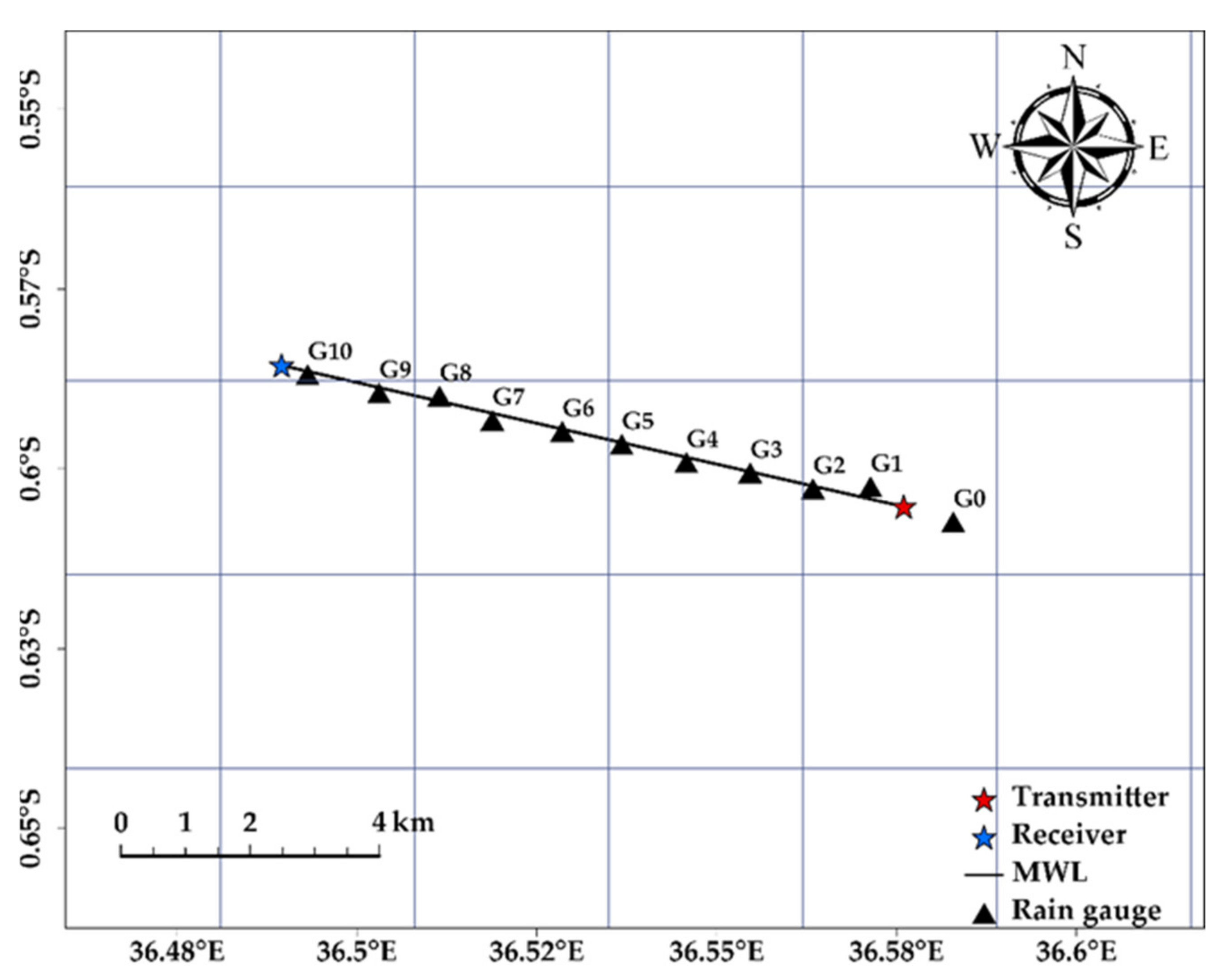
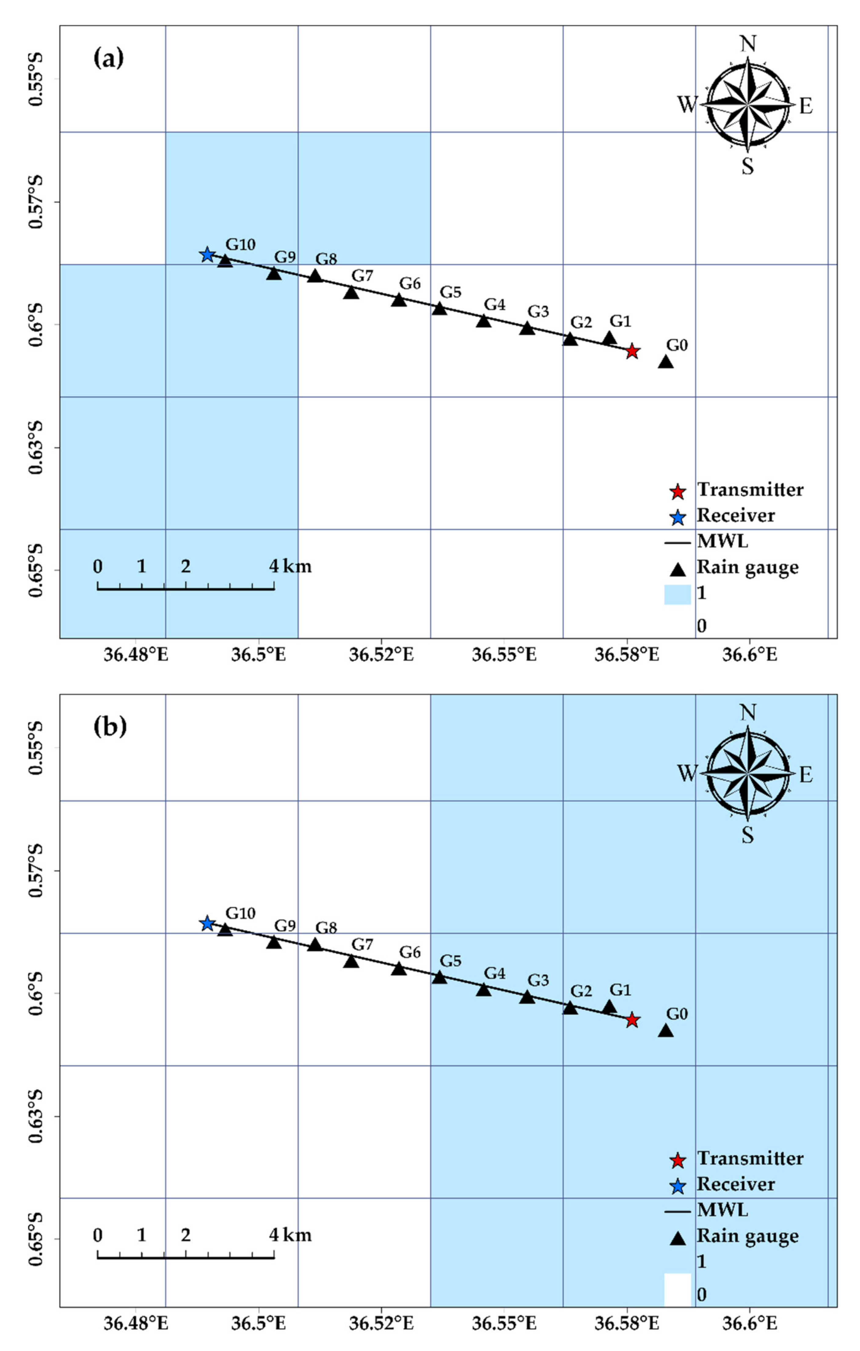
2. Study Area and Dataset

The data used in this study were MWL, rain gauges, and MSG SEVIRI from a topographically complex area (−0.61°S, 36.6°E) close to the Aberdare mountain in Kenya (0.02°S, 37.90°E). The evaluation period was between May–June 2018. Previous research conducted in this region and the evaluation period demonstrated the data’s capability for rainfall detection and estimation [11].

Rainfall data from nine aerodynamic ‘tipping buckets’ (ARG TB) rain gauges and two rain gauges from Trans-African Hydro-Meteorological Observatory (TAHMO) [32] served as ground truth in this study. The ARG TB were aligned under the MWL transect. In contrast, the TAHMO gauges were placed close to its transmitting and receiving antennas. The ARG TB logged data every minute using a Gemini Tinytag data logger, while the TAHMO gauges recorded rainfall data every 5 min. One tip of the ARG TB equates to 0.198 to 0.202 mm rain.

A Kenyan telecom service provider, Safaricom, supplied the received signal level (RSL) data for a 15 GHz, 9.88 km MWL. The RSL data were characterised by minimum, maximum, and mean values at 15 min intervals and a resolution of 0.1 dBm. It is an Aviat Eclipse MWL, vertically polarised, and has a constant transmitted signal level (TSL). The data was accessed through Safaricom’s head office in Nairobi, Kenya.

The MSG SEVIRI data was obtained from the Meteosat at 41.5°E, which corresponded to Meteosat 8 [33] when the data was retrieved. The SEVIRI channels used were visible (VIS0.6 μm) and near-infrared (NIR1.6 μm), provided by https://www.eumetsat.int/archived-meteosat-data (accessed on 16 June 2021) at 3 km and 15 min spatiotemporal resolution.

3. Method

3.1. Rainfall Intensities Estimated from Rain Gauges

The rainfall for all gauges was used to estimate rainfall intensities (R mm h⁻¹) at 15 min. For the ARG TB, this was computed from the per-minute rain rate in millimetres estimated from the tipping count and the gauge specific tip equivalent of rain in mm provided by the manufacturer. On the other hand, R (mm h⁻¹) from the TAHMO data were computed from their 5 min accumulated rain rates. In this study, a gauge was considered raining if the R (mm h⁻¹) was above 0.5 mm h⁻¹; otherwise, it was non-raining.

Table 1. Summary of non-zero rainfall intensities from all rain gauges.

	G0	G1	G2	G3	G4	G5	G6	G7	G8	G9	G10
Mean	7.12	7.65	8.74	8.25	6.79	4.41	2.88	4.36	6.7	3.82	3.98
Maximum	43.46	23.64	72.36	49.53	27.72	43.63	5.54	27.47	19.3	12.86	28.02
Standard deviation	9.8	7.65	15.01	12.79	8.16	8.56	1.43	5.61	7.33	3.98	5.71
Fraction%	3.29	1.72	2.4	1.98	1.46	2.82	1.14	2.47	0.62	0.82	1.88
N	70	7	23	19	14	44	11	46	6	8	40
n days	53	12	26	26	26	39	26	46	26	26	53

N is the total number of 15 min of rainfall data assembled from n number of days during the daytime in the evaluation period. The Fraction (%) represents the fraction of raining periods.

provides a summary of the non-zero rainfall data for all the gauges. The differences in the gauge rainfall data records are mainly due to spatial variability of rainfall in the area due to topography and gauge malfunctions during the field campaign. For instance, gauge G1 was often non-operational during the field campaign, thus having the least days with data records. Nonetheless, these gauge rainfall records depict high spatial variability of rainfall over the MWL propagation path.

3.2. Rainfall Intensities Estimated from MWL

The rain-induced specific attenuation $A$ (dB km⁻¹) can be used to estimated $R$ (mm h⁻¹) from, e.g., the power-law model in [24]:

$$\mathrm{A}=a{R}^b$$

(1)

where the $a$ ((dB km⁻¹) (mm h⁻¹)^−b) coefficient and $b$ (-) exponent depend on the MWL frequency, polarisation, and local rainfall climatology [19,24], which can be acquired from the literature, such as [34].

3.2.1. The Conventional Technique

The conventional technique used to estimate MWL rainfall intensities in this study is described in detail [11]. Here, a summary of the steps used to estimate the path average rainfall from the mean RSL data is provided. (1) The wet–dry classification of the MWL signal was by the rolling window approach, which uses the time series of the individual MWL signals separately. (2) Next, a reference or baseline level was estimated as the median of the mean RSL of the previous 24 h labelled as dry periods by the preceding step. Before computing $A$ from Equation (2), a dynamic model [25] was used to correct the mean RSL from attenuation due to antenna wetting.

$$A_{fp}=\frac{B-P}{L_{fp}}$$

(2)

where $A_{fp}$ (dB/km) is the rain-induced specific attenuation averaged over the entire MWL, $L_{fp}$ is the MWL length, and $B$ and $P$ are the baseline and the mean RSL, corrected for the effect of antenna wetting according to the dynamic model by [25]. Finally, Equation (3) estimated the R (mm h⁻¹) from $A_{fp}$.

$$R_{fp}={\left(\frac{A_{fp}}{a}\right)}^{\frac{1}{b}}$$

(3)

where $R_{fp}$ is the path average rainfall computed based on the entire MWL length, and $a \left(0.05008\right)$ and $b \left(1.0440\right)$ were from [34].

3.2.2. The New MSG Technique

The MSG technique incorporates an MSG-based rain area detection and correction method recently developed by [35] into the MWL rainfall estimation procedure. The method detects rain areas at 3 km and 30 min spatiotemporal resolution. However, in this study, it was implemented at MSG’s 15 min temporal resolution to match the temporal resolution of the MWL RSL data. Additionally, the method is capable of daytime and nighttime rain area detection, but this study focused on daytime detection due to its high success rate of rain detection. Further details of the method and its accuracy can be found in [35]; here, a summary and its application for MWL rainfall estimation are provided.

This rain area detection method is instantaneous, which means that, for each individual MSG scene, the method detects rain areas independent of the previous and subsequent scenes. It employs a parametric threshold model developed from a conceptual framework in which clouds characterised by top properties such as high top optical thickness and large effective radius have high rainfall probabilities and intensities. The daytime model is from MSG SEVIRI optical (VIS0.6) and near-infrared (NIR1.6) reflectance difference. Specifically, the model application assumes that a cloud is raining if the reflectance difference is above 0.21; otherwise, it is non-raining. The method subsequently corrects the detected rain areas by employing a gradient-based adaptive correction technique that uses rain area-specific parameters to reduce the number and sizes of the detected rain areas.

The following steps describe how the MSG-based rain area information is incorporated in the MSG technique for estimating rainfall intensities from the mean RSL data. (1) During each 15 min interval in the MWL mean RSL data, the rain area detection method classified the pixels over the link as raining or non-raining. When a pixel over the MWL was classified as raining, the new parameter, wpl, was retrieved from the length (km) of the MWL touching the raining pixel. Figure 1 displays the MSG pixels over and around the neighbourhood of the MWL.

A 15 min interval in the mean RSL data was classified as wet if the wpl was larger than 15% of the MWL length; otherwise, the interval was classified as dry. This was to ensure the retrieval of realistic path averaged specific attenuations values in the subsequent step. Simultaneously, the rainfall intensities measured by the rain gauges situated in the wpl were retrieved and averaged as the actual mean rainfall intensities. (2) After identifying the wet and dry period in the RSL data, the baseline level was estimated from the mean RSL. The latter is the median of the previous 24 h classified as dry by the MSG-based rain area detection technique. (3) Finally, the wet antenna correction method by [25] was implemented before estimating the rain-induced specific attenuation from:

$$A_{wp}=\frac{B_{MSG}-P}{L_{wp}}$$

(4)

where:

$A_{wp}$ (dB km⁻¹)—the rain-induced specific attenuation averaged over wpl

$L_{wp}$—the wpl (km) retrieved from the MSG-based rain area information

$B_{MSG}$—the baseline, retrieved from dry periods identified by the MSG-based rain area information. The average R (mm h⁻¹) was estimated from $A_{wp}$ using:

$$R_{wp}={\left(\frac{A_{wp}}{a}\right)}^{\frac{1}{b}}$$

(5)

where $R_{wp}$ (mm h⁻¹) represents the average rainfall intensity over wpl.

3.2.2.1. Conditions and Uncertainties in Estimating the $R_{wp}$

Some conditions under which the $R_{wp}$ may be uncertain and the approach used to retrieve more accurate estimates are described. The first is when the wpl is between 1.5 (the threshold MWL length used to make a wet–dry decision in the RSL data) and 3 km (i.e., the width of the MSG pixel). Figure 2a shows rain area detection over the MWL in binary classification (1 is rain and 0 is no rain) where wpl is approximately 2 km. The $R_{wp}$ for such wpl are high and do not correlate with the gauge rainfall and MSG pixel intensity, such as those from convective raining pixels, because the MWL attenuation is computed over a short MWL length. For these cases, the $R_{wp}$ from Equation (5) was multiplied by $\alpha =\frac{wpl}{L}$, where $\alpha$ < 1 and $L$ is the MWL length, to retrieve more accurate estimates. The second is when wpl is estimated from rain areas defined by mixed pixels (i.e., raining MSG pixels of varying reflectance difference intensities) from a convective rain cloud. A convective rain cloud covered few rain gauges (see Figure 2b), had high gauge rain intensities, and, mostly, lasted for less than an hour. The intensities of the raining area MSG pixels also varied from a maximum reflectance difference to a relatively low difference. To capture the high rain intensities for such raining cases requires determining the centre of the convective rainstorm. This was determined as the raining pixels with reflectance difference greater than mean reflectance difference of all raining pixels covering the MWL, and wpl was estimated from the length of the MWL covered by these pixels.

3.3. Error Metrics

The average rainfall intensities by the conventional and MSG technique were compared to the rain gauges using the root mean squared deviation (RMSD), relative bias (RB), and coefficient of determination (r²) to evaluate their performances against the actual mean rainfall intensities. The actual mean rainfall intensities for the conventional technique were computed from all gauges under the MWL; for the MSG technique, this was computed from gauges under wpl. Detailed descriptions for these metrics are in [36,37,38] and in Equations (6) and (7), respectively.

$$RMSD=\sqrt{\frac{{{\displaystyle \sum }}_{i=1}^N{\left(R_{Mi}-R_{RGi}\right)}^2}{N}}$$

(6)

$$RB=\frac{\frac{1}{N}*{{\displaystyle \sum }}_{i=1}^N\left(R_{Mi}-R_{RGi}\right)}{\frac{1}{N}*{{\displaystyle \sum }}_{i=1}^N{R}_{RGi}}$$

(7)

where $R_{Mi}$ represents all possible MWL rainfall intensity estimates by the conventional and MSG technique, $R_{RGi}$ represents all possible gauge mean rainfall estimates, and N is the number of samples.

4. Results

This section compares the MWL rainfall intensity estimates by the conventional and the new MSG technique to actual mean rainfall intensities from gauges to evaluate the new technique’s accuracy for improving MWL rainfall intensity estimates. From the raw mean RSL to the MWL rainfall intensity estimates, line plots for specific rainy periods were used to compare MWL rainfall intensity estimates to rain gauge estimates. The selected periods, due to their variable rain intensities observed, allowed for an effective visual comparison of the new MSG and conventional techniques. Finally, performance metrics computed based on all the 15 min intervals in the MWL RSL data evaluate the accuracy of the new technique for MWL rainfall intensity estimation.

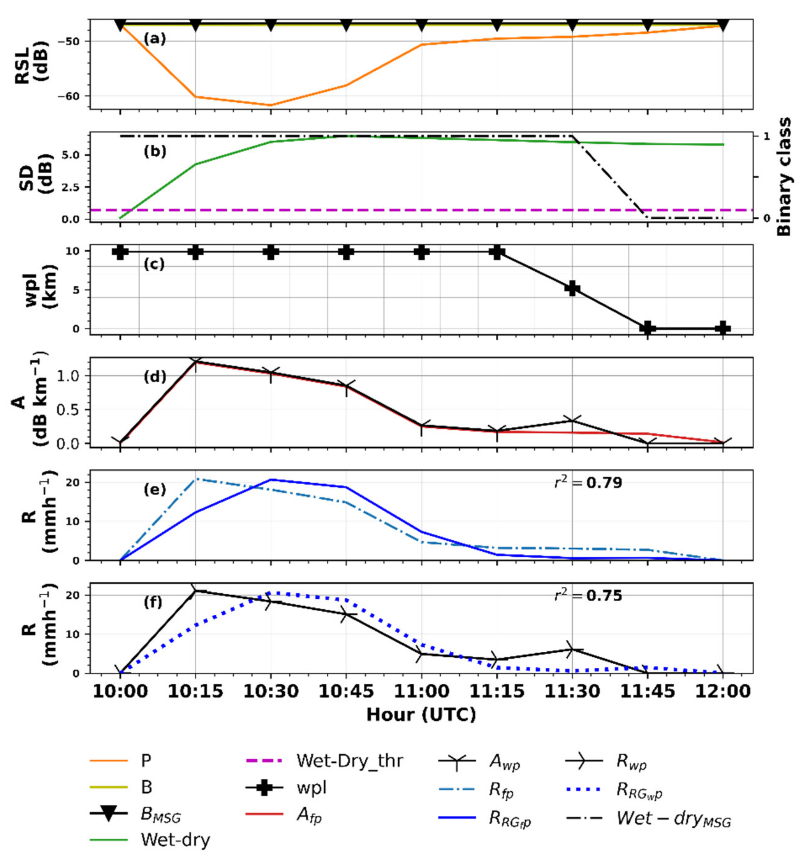
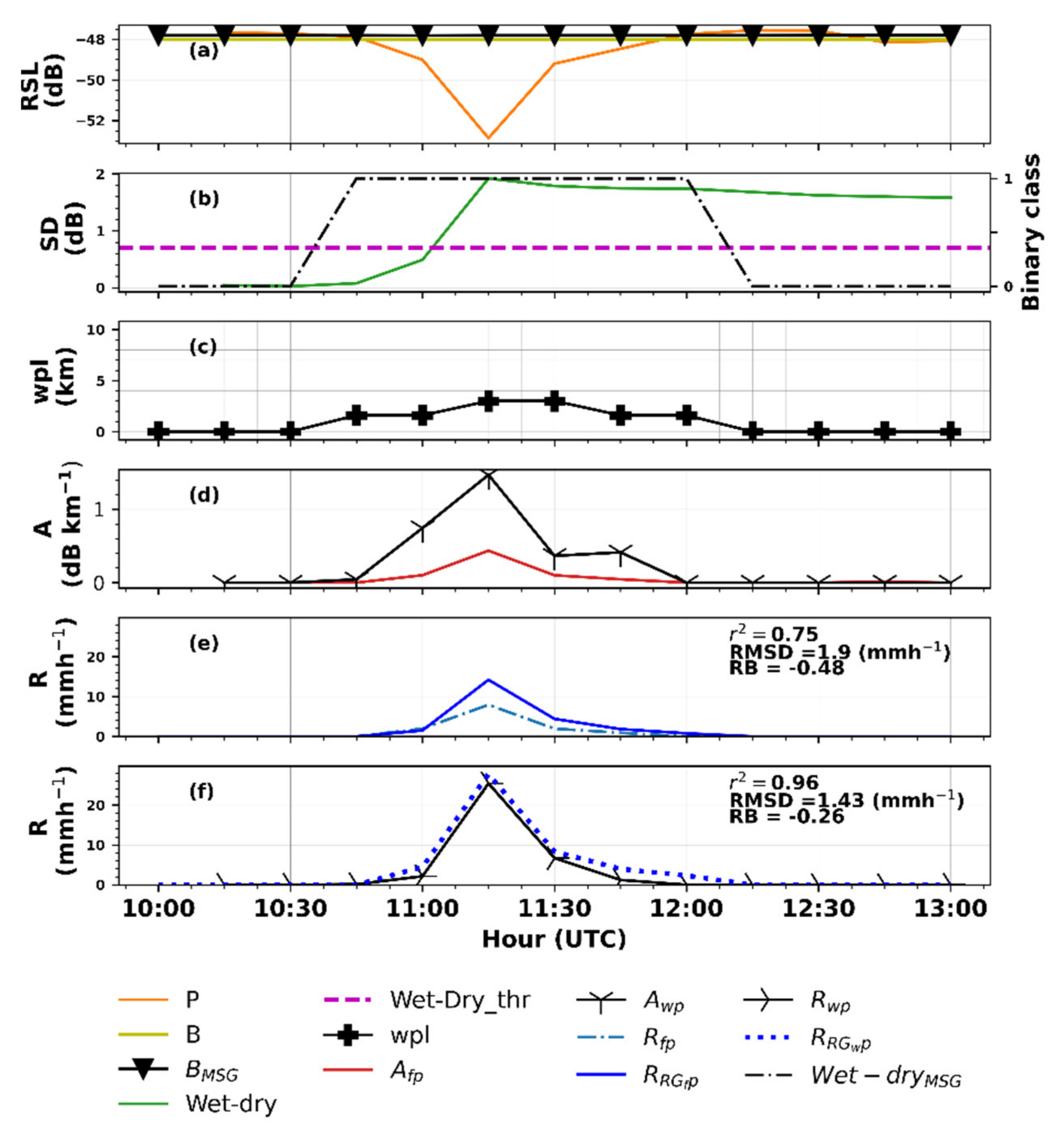
4.1. From Raw RSL to Rainfall Intensity Estimates: A Comparison of the Conventional and MSG Technique

Figure 3 demonstrates the transformation of the mean RSL to rainfall intensities and its comparison with the actual mean intensities from rain gauges according to the conventional and MSG techniques. Figure 3a shows comparable baseline levels estimates by the conventional and MSG techniques. Figure 3b compares wet–dry classification by the conventional and MSG technique. The dashed pink line indicates a standard deviation threshold value of 0.7 (dB), an empirically determined value by [11], that separates the wet (above 0.7 dB) and dry (below 0.7 dB) in the conventional technique. Instead, the MSG technique uses a binary classification of 0 and 1 to indicate when the MWL is wet (1) and dry (0).

From Figure 3b, one can observe comparable wet–dry classification estimates by the two techniques. For wet intervals above 0.7 (dB) in the conventional technique, the MSG technique flagged those intervals as wet. These observations mostly coincide with the decrease in mean RSL (dB) in Figure 3a, attributed to rainfall occurrences identified by the rain gauges. Nonetheless, unlike the MSG technique, the conventional wet–dry classification occasionally detects wet periods even when it has ceased, e.g., after 11:45, which may be due to the effect of antenna wetting after a rain event.

According to the wpl in Figure 3c, the MWL was fully wet from the onset of the rain event till 11:15 and then partially wet at 11:30. Thus, this suggests that the rain events during the former periods occurred over the entire MWL length, whereas for the latter period, the event occurred over approximately half the MWL length.

Following these observations, one can observe comparable rain-induced specific attenuation estimates (Figure 3d) by the conventional and MSG techniques from the rain event onset till 11:15 since their attenuation estimates were computed over the entire MWL length. In contrast, the attenuation estimate at 11:30 was comparatively higher for the MSG because, unlike the conventional technique, it was estimated over a shorter MWL length (approximately 5 km). The MWL rainfall intensities by the conventional and MSG techniques in Figure 3e,f, respectively, were comparable most of the time for this rain event. Overall, they had a convincing agreement with the actual mean rainfall intensities from the rain gauges according to the r² values computed based on the entire rain event period. One observable feature in Figure 3e,f is that both the conventional and MSG techniques overestimated the actual mean intensities at the onset of the rainfall event.

Figure 4, like Figure 3, demonstrates the transformation of the mean RSL to rainfall intensities by the conventional and MSG techniques compared to the actual mean rainfall intensities from rain gauges. The baseline level by both techniques in Figure 4a again shows comparable estimates.

Their wet–dry classifications (Figure 4b) are also primarily comparable, especially for wet periods between 11:00 and 12:00. As was observed in Figure 3, these observations coincide with a decrease in mean RSL (dB) attributed to rainfall as observed by the rain gauges. However, there are some differences in Figure 4b. The wet–dry classification by the MSG technique seems to detect wet periods before the onset of the wet period, which does not agree with the mean RSL and the no rainfall occurrence in the rain gauges, e.g., between 10:30 and 10:45. On the other hand, the conventional technique missed the onset of the wet periods between 10:45 and 11:00. For the MSG technique, this may be due to the raining cloud top properties available before the onset of the rain event, which resulted in false rain detection by the rain detection method used by the MSG wet–dry classification technique. By contrast, the conventional wet–dry technique missing the beginning of the wet period may be due to low rainfall intensities that resulted in a mean RSL that is not entirely different from RSL in the preceding dry periods. Again, the conventional technique continues to report wet periods even after it has ceased, likely due to the wet antenna effect.

Figure 4c suggests spatiotemporally distributed rainfall events occurred along the MWL length, indicated by time-varying wpl, for the entire raining period. Such rainfall events are often attributed to convective rainfall and are associated with subhourly high rain intensities. In Figure 4d, the MSG technique estimated comparatively high attenuations than the conventional technique because it was estimated over a portion of the MWL length rather than the entire length (i.e., according to the conventional technique).

As shown in Figure 4e,f, the rainfall intensities by the MSG technique are also comparatively higher than the conventional technique due to its higher attenuation estimates. Its rainfall intensity estimates better reflect the high rainfall intensities observed for that rainfall event and compare better to its actual mean rainfall than the conventional technique according to the error metrics shown in the figures. This can be attributed to determining the rainstorm’s centre for a more accurate estimation of wpl to capture the high rainfall intensities.

Figure 5 is an analogous comparison of Figure 3 and Figure 4, but for different date–time periods. Again, Figure 5a shows comparable baseline levels estimates by the MSG and conventional techniques. The wet–dry classification in Figure 5b shows that the MSG technique captures the dynamics in the mean RSL and rainfall observation in the rain gauges better than the conventional technique. It is clear from the figure that the technique coincides nicely with the onset and end of the wet period and the dry periods preceding and after the wet periods. On the other hand, the conventional technique missed the onset of the wet period and continued to detect wet periods even after it has ceased.

The wpl showed in Figure 5c suggests spatiotemporally varying rainfall events occurred along the MWL length, as in the previous analysis (Figure 4c). Correspondingly, Figure 5d shows comparatively higher attenuation estimates by the MSG than the conventional technique. This is because it was estimated over varying portions of the MWL rather than the entire length based on the conventional technique. According to their figures’ error metrics, their rainfall estimates in Figure 5e,f show good agreement with the actual mean rainfall estimates from the gauges, albeit better in the MSG than the conventional technique.

Albeit analogous to previous figures, Figure 6 is a unique comparison of the MSG and conventional technique regarding frequent gaps in the MWL RSL data. The mean RSL in Figure 6a shows that the MWL data was available for only a few minutes of this rainfall event. For this reason, wet–dry classification, attenuation, and rainfall (Figure 6b,d,e, respectively) were not successful in the conventional technique. However, the MSG technique determines the wet–dry periods and wpl instantaneously from the rain areas information (Figure 6b,c). Therefore, the technique could estimate attenuation and rainfall intensities (Figure 6d,f, respectively) for the period when the MWL data was available. Note here that the r² values are not computed in Figure 6e,f because the MWL data gaps did not allow for a fair comparison of MWL–gauge rainfall intensities.

Figure 7 demonstrates the effect of $\alpha$ in correcting the $R_{wp}$ described in Section 3.2.2.1. As shown in Figure 7b,d,e, the conventional technique missed this period’s rain event, possibly due to the low rain rates (< 5 mm h⁻¹) observed based on the gauge rainfall data. The MSG technique’s wet–dry classification detected the event (Figure 7b), which may be attributed to the MSG-based rain area detection’s ability to detect low rain rates. The wpl in 7c shows the time-varying MWL length covered by the rain. For instance, at the beginning and end of the event, the estimated wpl was < 3 km. Subsequently, the attenuation and rainfall retrieved based on this MWL length were high and did not agree with the gauge rainfall intensities, thus requiring correction. After correction using the $\alpha$, the MSG technique’s rainfall intensities $R_{wp-corrected}$, visually shows a better agreement with the observed rainfall intensities by the rain gauges than its previous estimate based on the wpl.

Overall, the results show that rainfall estimation from MWL is robust in approximating the actual mean rainfall intensities over the MWL propagation path. Additionally, the MSG technique was successful in estimating wet–dry and baseline level MSG techniques. This can be attributed to the MSG-based rain area detection, which uses relevant information content on cloud-top properties and rainfall available in the VIS 0.6 and NIR 1.6 reflectance pair. In particular, the successful baseline level estimates by the MSG technique can be attributed to the robustness of the MSG data in detecting dry areas [11]. Furthermore, the new parameter, wpl, derived from the MSG-based rain area information, effectively estimated attenuation and, subsequently, rainfall intensities comparable to the conventional and actual gauge estimates, especially when the entire MWL length was wet. Based on the results, it can also be stated that, when the rainfall is not spatially covering the entire length of the MWL, the MSG technique provides a better estimate of the actual mean rainfall as retrieved from, e.g., rain gauges.

4.2. Appraisal of the MSG and Conventional Technique for MWL Rainfall Intensity Estimation

Table 2. Error metrics computed for varying evaluation timestamps.

Estimation technique	RMSD mm h−1				RB				r2
	15 min	30 min	1 h	3 h	15 min	30 min	1 h	3 h	15 min	30 min	1 h	3 h
MSG technique	0.63	0.84	1.32	2.61	0.47	0.47	0.47	0.47	0.70	0.78	0.83	0.81
Conventional technique	0.60	0.80	1.23	2.09	0.02	0.02	0.03	0.04	0.63	0.73	0.80	0.84

The total number of MWL–gauge rainfall intensity pairs (including raining >0.5 mm h⁻¹ and non-raining <0.5 mm h⁻¹) that computed the error metrics were 2088, 1380, 660, and 240 for the evaluation timestamps at 15, 30 min, one hour, and three hours, respectively, covering the evaluation period. Note that these data and periods corresponded to when the MWL, MSG satellite, and rain gauges coincided.

presents the error metrics computed based on MWL and gauge rainfall intensity pairs for evaluation timestamps at 15 min, 30 min, hourly, and every three hours for both the MSG and conventional techniques. The RB suggest an overestimation of rainfall intensities by the MWL relative to the actual gauge estimates, albeit comparatively higher in the MSG than the conventional technique. This is reflected in the RMSD, which is comparable for the two techniques, except for the scores every three hours. Nonetheless, their r² values were above 0.5 at 15 min, which increased due to aggregation [39] above 0.8 at evaluation timestamps every hour, and three hours, indicating that both techniques can estimate gauge comparable rainfall intensities.

Various factors may account for the overestimation of rainfall intensities by the MWL relative to the gauge estimates. The MWL rainfall intensities represent areal average estimates derived from 15 min instantaneous mean RSL data, whereas the gauge computed areal average rainfall estimates from point measurements recorded at per minute and 5 min intervals. Additionally, spatial variability of rainfall in the study area and uncertainties in the MWL rainfall estimation may contribute to the discrepancies between the MWL and gauge estimates [11,40].

In particular, the comparatively high overestimation by the MSG, compared to the conventional technique, is mainly attributed to uncertainties in the MSG-based rain area detection [35]. For instance, false alarms in the rain area detection method could significantly affect the wet–dry classification and baseline level estimation. A dry interval in the MWL data, incorrectly identified by the MSG-based information as wet, could compute rainfall for a dry period and impact the RMSD and RB scores. Furthermore, the MSG technique estimated high attenuation and rainfall intensities for wpl less than the MWL length (indicating spatial variability of rainfall over the MWL). Additionally, this wpl is tied to the MSG rain area information’s accuracy and may further impact the computed error metrics that evaluate the MSG technique’s accuracy.

5. Discussion

A new technique for MWL rainfall estimation is investigated and described using a 15 GHz, 9.88 km MWL, and MSG SEVIRI VIS0.6 μm and NIR1.6 μm satellite data. The investigation, conducted during the daytime, used the MSG data for detecting rain areas, according to the method by [35], over the MWL propagation path. This spatial information on rain areas provided by the MSG data estimated three significant parameters: wet–dry periods, baseline level, and wpl for estimating MWL rainfall intensities.

All three parameters were estimated instantaneously from the MSG satellite data. The wet–dry periods indicate periods when the MWL was wet or dry, whereas the baseline level represented the MWL’s behaviour in the dry period. The wpl is a property of the MWL’s length, and it indicates the approximate length of the MWL during a wet period based on which the rain-induced attenuation was estimated. Eventually, rainfall intensity was estimated using all parameters, and the results were compared to intensities estimated by a conventional method and rain gauges (where the gauge served as the actual estimates).

The results demonstrate an effective skill of the new MSG technique. The wet–dry periods and baseline level estimates were comparable to those of the conventional technique. In addition, the wpl effectively estimated the MWL signal attenuations for wet periods, and subsequently, the rainfall estimates agreed well with the conventional and rain gauge estimates when the rainfall was spatially covering the entire length of the MWL (i.e., when the wpl was equal to the MWL length). However, when the rainfall is convective and spatially covered a portion of the MWL, determining the centre of the rainstorm is required to estimate a more accurate wpl and capture the high rainfall intensities that reflect the actual mean intensities better than the conventional technique. Moreover, unlike the conventional technique, the MSG technique’s rainfall detection and estimation were unaffected by periods with no MWL RSL measurement.

Furthermore, the current study’s results were better than the previous study’s results [11] for the same link, albeit with overestimation. The hourly RB and r² values were –0.18 and 0.58, respectively, estimated from daytime and nighttime rainfall combined. The differences in performance may be due to the daytime rainfall and its high rainfall intensities measured by this current study, for which the influence of wet antenna and wet–dry classification errors may be minimal [41]

The MSG technique showed high RB and RMSD scores compared to the conventional technique. Generally, the differences can be attributed to factors such as the differences in their measurement techniques and uncertainties in the MWL rainfall estimation procedure. The differences resulting from the uncertainties in the rain area detection provided by the MSG, such as false rain detections, could be interpreted in the MWL data as wet periods and be used to compute rainfall during dry periods, impacting the metric scores. It is noteworthy that this study’s results were based on daytime MSG satellite reflectance data. Additionally, convective clouds with cold cloud top temperatures are responsible for most of the rainfall in the area. Therefore, our analysis did not consider the overall effect of warm rainfall, i.e., rain from clouds with top temperatures warmer than 273 K [42,43]. However, nighttime applications and applications with rain areas derived from thermal infrared satellite data, e.g., [42], warm rains, may further impact the error metrics. For instance, the MSG technique may underestimate the actual mean rainfall estimates for warm rains that are not detected by the satellite-based rain area information.

The study’s results may have many implications. For instance, the successful wet–dry classification and baseline level estimation by this MSG technique indicates that it may be applied when the conventional technique is limited. In particular, since their estimation is independent of the MWL RSL data and instantaneous from the satellite data, it may not be affected by the MWL network density or sampling frequency of the MWL RSL data, which are common to the conventional technique. Additionally, wpl could estimate mean rainfall intensities more reflective of the actual mean rainfall intensities. This fact indicates that spatial variability of rainfall along the MWL (as shown in Section 3.1) may be essential information to consider in the MWL rainfall estimation. More detailed information on the rainfall process and type (such as convective, stratiform) from the satellite, e.g., [43,44], may also inform the $a$ and $b$ parameters in Section 3.2, because these parameters may differ according to the rainfall type, e.g., convective rainfall [24], and may improve the MWL rainfall estimates. An overall implication of the success of this MSG technique based on this study’s results is that the MWL MSG synergy may be beneficial for large scale rainfall estimation and monitoring or complement existing techniques.

Despite the new MSG technique’s robustness and accurate rainfall estimates, further studies are needed, for instance, using multiple MWL. Additionally, wpl needs further investigation, especially for wpl less than the width of the MSG pixel (i.e., ~3 km). Furthermore, from a scientific research perspective, it is necessary to estimate and validate wpl using other remote sensing systems such as weather radars. In fact, radars may provide better estimates since they can provide rainfall locations more accurate than those derived using cloud-top information from geostationary satellites such as MSG. These questions constitute our future research.

6. Conclusions

A new MSG technique for MWL rainfall estimation was presented, which incorporates rain areas detections by MSG satellite for the MWL rainfall retrievals. Based on the presented results, the technique is robust and is capable of wet–dry, baseline, and gauge comparable rainfall intensity estimates to benefit many operational and research applications. Specifically, the results confirm the capability of the MWL to estimate accurate mean rainfall estimates that had occurred over the MWL propagation path, especially when the rainfall occurred over the entire MWL path. However, when rainfall is spatially varying over the MWL (often the case for high-intensity convective rainfall), the results suggest that the MSG technique may approximate the actual mean rainfall better than the conventional technique.

Nevertheless, the technique is limited because its accuracy is linked to the spatial information on rain areas provided by the MSG satellite data. Nonetheless, this limitation may be prevented to some extent by using more accurate information from remote sensors such as weather radars. The study’s results are from a single 15 GHz, 9.88 km MWL with two months of gauge, MWL, and satellite data. Despite this limitation, the results improve the MWL rainfall estimation specifically from the perspective of a spatially varying rainfall occurrence. Additionally, we show that the satellite information is capable of wet–dry and baseline level estimation, which may benefit large scale application of the MWL and satellite for rainfall retrievals.

Overall, the new MSG technique may largely contribute to rainfall estimation and monitoring in many ungauged areas where the MWL and satellite data are readily available. In particular, its application for estimating high rainfall intensities from convective systems may benefit many applications in flash flood warnings and the nowcasting of hazardous storms.

References

1. Patrick, S. Microwave Link: Gigabit Microwave Connectivity. Available online: https://www.microwave-link.com/ (accessed on 13 July 2021).
2. Ericsson. Ericsson Microwave towards 2020: Delivering High-Capacity and Cost-Efficient Backhaul for Broadband Networks Today and in the Future; Ericsson: Stockholm, Sweden, 2015. [Google Scholar]
3. Edstam, J.; Olsson, A.; Flodin, J.; Öhberg, M.; Henriksson, A.; Hansryd, J.; Ahlberg, J. Ericsson Microwave Outlook; Ericsson: Göteborg, Sweden, 2018. [Google Scholar]
4. Leijnse, H.; Uijlenhoet, R.; Stricker, J.N.M. Hydrometeorological Application of a Microwave Link: 2. Precipitation. Water Resour. Res. 2007, 43, 1–9. [Google Scholar] [CrossRef]
5. Messer, H.; Zinevich, A.; Alpert, P. Environmental monitoring by wireless communication networks. Science 2006, 312, 713. [Google Scholar] [CrossRef] [Green Version]
6. Overeem, A.; Leijnse, H.; Uijlenhoet, R. Measuring urban rainfall using microwave links from commercial cellular communication networks. Water Resour. Res. 2011, 47, 1–16. [Google Scholar] [CrossRef]
7. David, N.; Alpert, P.; Messer, H. The potential of cellular network infrastructures for sudden rainfall monitoring in dry climate regions. Atmos. Res. 2013, 131, 13–21. [Google Scholar] [CrossRef]
8. David, N.; Liu, Y.; Kumah, K.K.; Hoedjes, J.C.B.; Su, B.Z.; Gao, H.O. On the Power of Microwave Communication Data to Monitor Rain for Agricultural Needs in Africa. Water 2021, 13, 730. [Google Scholar] [CrossRef]
9. David, N.; Gao, H.O.; Kumah, K.K.; Hoedjes, J.C.B.; Su, Z.; Liu, Y. Microwave communication networks as a sustainable tool of rainfall monitoring for agriculture needs in Africa. In Proceedings of the 16th International Conference on Environmental Science and Technology, Rhodes, Greece, 4–7 September 2019. [Google Scholar]
10. Doumounia, A.; Gosset, M.; Cazenave, F.; Kacou, M.; Zougmore, F. Rainfall monitoring based on microwave links from cellular telecommunication networks: First results from a West African test bed. Geophys. Res. Lett. 2014, 41, 6016–6022. [Google Scholar] [CrossRef]
11. Kumah, K.K.; Hoedjes, J.C.B.; David, N.; Maathuis, B.P.; Gao, H.O.; Su, B.Z. Combining MWL and MSG SEVIRI Satellite Signals for Rainfall Detection and Estimation. Atmosphere 2020, 11, 884. [Google Scholar] [CrossRef]
12. Overeem, A.; Leijnse, H.; Uijlenhoet, R. Country-wide rainfall maps from cellular communication networks. Proc. Natl. Acad. Sci. USA 2013, 110, 2741–2745. [Google Scholar] [CrossRef] [PubMed] [Green Version]
13. Overeem, A.; Leijnse, H.; Uijlenhoet, R. Two and a half years of country-wide rainfall maps using radio links from commercial cellular telecommunication networks. Water Resour. Res. 2016, 52, 8039–8065. [Google Scholar] [CrossRef] [Green Version]
14. Rahimi, A.R.; Upton, G.J.G.; Holt, A.R. Dual-frequency Links—A Complement to Gauges and Radar for the Measurement of Rain. J. Hydrol. 2004, 288, 3–12. [Google Scholar] [CrossRef]
15. Chwala, C.; Kunstmann, H. Commercial microwave link networks for rainfall observation: Assessment of the current status and future challenges. Wires Water 2019, 6, e1337. [Google Scholar] [CrossRef] [Green Version]
16. Upton, G.J.G.; Holt, A.R.; Cummings, R.J.; Rahimi, A.R.; Goddard, J.W.F. Microwave Links: The Future for Urban Rainfall Measurement? Atmos. Res. 2005, 77, 300–312. [Google Scholar] [CrossRef]
17. Zinevich, A.; Alpert, P.; Messer, H. Estimation of rainfall fields using commercial microwave communication networks of variable density. Adv. Water Resour. 2008, 31, 1470–1480. [Google Scholar] [CrossRef]
18. Leijnse, H.; Uijlenhoet, R.; Stricker, J.N.M. Microwave link rainfall estimation: Effects of link length and frequency, temporal sampling, power resolution, and wet antenna attenuation. Adv. Water Resour. 2008, 31, 1481–1493. [Google Scholar] [CrossRef]
19. Uijlenhoet, R.; Overeem, A.; Leijnse, H. Opportunistic remote sensing of rainfall using microwave links from cellular communication networks. Wires Water 2018, 5, e1289. [Google Scholar] [CrossRef] [Green Version]
20. David, N.; Sendik, Q.; Messer, H.; Alpert, P. Cellular network infrastructure: The future of fog monitoring? Bull. Am. Meteorol. Soc. 2015, 96, 1687–1698. [Google Scholar] [CrossRef]
21. Overeem, A.; Leijnse, H.; Uijlenhoet, R. Retrieval algorithm for rainfall mapping from microwave links in a cellular communication network. Atmos. Meas. Tech. 2016, 9, 2425–2444. [Google Scholar] [CrossRef] [Green Version]
22. Schleiss, M.; Berne, A. Identification of Dry and Rainy Periods Using Telecommunication Microwave Links. IEEE Geosci. Remote Sens. Lett. 2010, 7, 611–615. [Google Scholar] [CrossRef]
23. Gaona, M.F.R.; Overeem, A.; Leijnse, H.; Uijlenhoet, R. Measurement and interpolation uncertainties in rainfall maps from cellular communication networks. Hydrol. Earth Syst. Sci. 2015, 19, 3571–3584. [Google Scholar] [CrossRef] [Green Version]
24. Olsen, R.; Rogers, D.; Hodge, D. The aRb Relation in the Calculation of Rain Attenuation. IEEE Trans. Antennas Propag. 1978, 26, 318–329. [Google Scholar] [CrossRef]
25. Schleiss, M.; Rieckermann, J.; Berne, A. Quantification and modeling of wet-antenna attenuation for commercial microwave links. IEEE Geosci. Remote Sens. Lett. 2013, 10, 1195–1199. [Google Scholar] [CrossRef]
26. Nakamura, M. Method for wet antenna correct at 50 GHz. J. Chem. Inf. Modeling 2013, 53, 1689–1699. [Google Scholar] [CrossRef]
27. Villarini, G.; Mandapaka, P.V.; Krajewski, W.F.; Moore, R.J. Rainfall and sampling uncertainties: A rain gauge perspective. J. Geophys. Res. Atmos. 2008, 113, D11102. [Google Scholar] [CrossRef]
28. Schmetz, J.; Pili, P.; Tjemkes, S.; Just, D.; Kerkmann, J.; Rota, S.; Ratier, A. An Introduction to Meteosat Second Generation (MSG). Bull. Am. Meteorol. Soc. 2002, 83, 977–992. [Google Scholar] [CrossRef]
29. Kuhnlein, M.; Thies, B.; Nauss, T.; Bendix, J. Rainfall-Rate Assignment Using MSG SEVIRI Data-A Promising Approach to Spaceborne Rainfall-Rate Retrieval for Midlatitudes. J. Appl. Meteorol. Climatol. 2010, 49, 1477–1495. [Google Scholar] [CrossRef]
30. Van het Schip, T.I.; Overeem, A.; Leijnse, H.; Uijlenhoet, R.; Meirink, J.F.; van Delden, A.J. Rainfall measurement using cell phone links: Classification of wet and dry periods using geostationary satellites. Hydrol. Sci. J. 2017, 62, 1343–1353. [Google Scholar] [CrossRef]
31. Hoedjes, J.C.B.; Kooiman, A.; Maathuis, B.H.P.; Said, M.Y.; Becht, R.; Limo, A.; Mumo, M.; Nduhiu-Mathenge, J.; Shaka, A.; Su, B. A Conceptual Flash Flood Early Warning System for Africa, Based on Terrestrial Microwave Links and Flash Flood Guidance. ISPRS Int. J. Geo Inf. 2014, 3, 584–598. [Google Scholar] [CrossRef] [Green Version]
32. Van de Giesen, N.; Hut, R.; Selker, J. The Trans-African Hydro-Meteorological Observatory (TAHMO). Wiley Interdiscip. Rev. Water 2014, 1, 341–348. [Google Scholar] [CrossRef] [Green Version]
33. Eumetsat. Meteosat-8 Satellite’s New Position of 41.5E Provides Weather and Climate View over the Indian Ocean. Available online: https://phys.org/news/2016-09-meteosat-satellite-position-415e-weather.html (accessed on 14 July 2020).
34. ITU. Specific Attenuation Model for Rain for Use in Prediction Methods; I.T.U. RECOMMENDATION ITU-R P.838-3; ITU: Geneva, Switzerland, 2005. [Google Scholar]
35. Kingsley, K.K.; Maathuis, B.H.P.; Hoedjes, J.C.B.; Rwasoka, D.T.; Retsios, B.V.; Su, B.Z. Rain Area Detection in South-Western Kenya by Using Multispectral Satellite Data from Meteosat Second Generation. Sensors 2021, 21, 3547. [Google Scholar] [CrossRef]
36. Wilks, D.S. Statistical Methods in the Atmospheric Sciences; Academic Press: London, UK, 2006; Volume 14, p. 627. [Google Scholar]
37. Walther, B.A.; Moore, J.L. The concepts of bias, precision and accuracy, and their use in testing the performance of species richness estimators, with a literature review of estimator performance. Ecography 2005, 28, 815–829. [Google Scholar] [CrossRef]
38. Barnston, A.G. Correspondence among the Correlation, Rmse, and Heidke Forecast Verification Measures—Refinement of the Heidke Score. Weather Forecast. 1992, 7, 699–709. [Google Scholar] [CrossRef] [Green Version]
39. Rowe, R.D. The Effects of Aggregation over Time on T-Ratios and R2’s. Int. Econ. Rev. 1976, 17, 751. [Google Scholar] [CrossRef]
40. Leijnse, H.; Uijlenhoet, R.; Berne, A. Errors and Uncertainties in Microwave Link Rainfall Estimation Explored Using Drop Size Measurements and High-Resolution Radar Data. J. Hydrometeorol. 2010, 11, 1330–1344. [Google Scholar] [CrossRef] [Green Version]
41. Overeem, A.; Leijnse, H.; van Leth, T.; Bogerd, L.; Priebe, J.; Tricarico, D.; Droste, A.M.; Uijlenhoet, R. Tropical rainfall monitoring with commercial microwave links in Sri Lanka. Environ. Res. Lett. 2021, 16, 074058. [Google Scholar] [CrossRef]
42. Feidas, H.; Giannakos, A. Identifying precipitating clouds in Greece using multispectral infrared Meteosat Second Generation satellite data. Theor. Appl. Climatol. 2011, 104, 25–42. [Google Scholar] [CrossRef]
43. Thies, B.; Nauss, T.; Bendix, J. Precipitation process and rainfall intensity differentiation using Meteosat Second Generation Spinning Enhanced Visible and Infrared Imager data. J. Geophys. Res. Atmos. 2008, 113, D23206. [Google Scholar] [CrossRef]
44. Thies, B.; Nauss, T.; Bendix, J. First results on a process-oriented rain area classification technique using Meteosat Second Generation SEVIRI nighttime data. Adv. Geosci. 2008, 16, 63–72. [Google Scholar] [CrossRef] [Green Version]
Figure 1. The MWL and rain gauges displayed in MSG pixels.
Remotesensing 13 03274 g001
Figure 2. Rain area detection over the MWL and wpl for different wet periods. (a) Rain areas covering approximately 20% of the MWL length (b) Rain areas covering approximately 50% of the MWL length The Blue (1) areas show raining areas and the white (0) are dry areas detected by the MSG-based rain area detection.
Remotesensing 13 03274 g002
Figure 3. From MWL mean RSL to rainfall for 15 min interval rain events of 8 May 2018. (a) compares the conventional ( B ) and MSG technique ( B M S G ) baseline level to the mean RSL ( P ), (b) compares wet–dry classification by the conventional (wet–dry) and MSG technique (wet–dryMSG)—the standard deviation threshold (wet–dry_thr, dashed pink line) value (0.7 dB) separates the wet and dry periods in the conventional technique; a binary class showing raining (1) and non-raining (0) periods separates the wet and dry periods in the MSG technique—(c) is the wpl over which the MSG technique computed attenuation ( A w p ), (d) compares the conventional ( A f p ) and MSG technique ( A w p ) attenuation, (e) compares the conventional MWL rainfall intensity ( R f p ) and the actual mean rainfall intensity ( R R G f p ), and (f) compares the MSG technique MWL rainfall intensity ( R w p ) and actual mean rainfall intensity ( R R G w p ).
Remotesensing 13 03274 g003
Figure 4. (af) As in Figure 3 but for 15 min interval rain events of 2 June 2018.
Remotesensing 13 03274 g004
Figure 5. (af) As in Figure 3 but for 15 min interval rain events of 9 June 2018.
Remotesensing 13 03274 g005
Figure 6. (af) As in Figure 3 but for 15 min interval rain events of 3 May 2018.
Remotesensing 13 03274 g006
Figure 7. (af) As in Figure 3 but for 15 min interval rain events of 15 May 2018.
Remotesensing 13 03274 g007