Improved Classification Models to Distinguish Natural from Anthropic Oil Slicks in the Gulf of Mexico: Seasonality and Radarsat-2 Beam Mode Effects under a Machine Learning Approach

Abstract

Distinguishing between natural and anthropic oil slicks is a challenging task, especially in the Gulf of Mexico, where these events can be simultaneously observed and recognized as seeps or spills. In this study, a powerful data analysis provided by machine learning (ML) methods was employed to develop, test, and implement a classification model (CM) to distinguish an oil slick source (OSS) as natural or anthropic. A robust database containing 4916 validated oil samples, detected using synthetic aperture radar (SAR), was employed for this task. Six ML algorithms were evaluated, including artificial neural networks (ANN), random forest (RF), decision trees (DT), naive Bayes (NB), linear discriminant analysis (LDA), and logistic regression (LR). Using RF, the global CM achieved a maximum accuracy value of 73.15. An innovative approach evaluated how external factors, such as seasonality, satellite configurations, and the synergy between them, limit or improve OSS predictions. To accomplish this, specific classification models (SCMs) were derived from the global ones (CMs), tuning the best algorithms and parameters according to different scenarios. Median accuracies revealed winter and spring to be the best seasons and ScanSAR Narrow B (SCNB) as the best beam mode. The maximum median accuracy to distinguish seeps from spills was achieved in winter using SCNB (83.05). Among the tested algorithms, RF was the most robust, with a better performance in 81% of the investigated scenarios. The accuracy increment provided by the well-fitted models may minimize the confusion between seeps and spills. This represents a concrete contribution to reducing economic and geologic risks derived from exploration activities in offshore areas. Additionally, from an operational standpoint, specific models support specialists to select the best SAR products and seasons for new acquisitions, as well as to optimize performances according to the available data.

1. Introduction

1.1. Natural and Anthropic Oil Slicks in the Gulf of Mexico

Oil and gas can reach the sea surface by leaking directly from either geological faults at the seafloor or from man-made facilities, such as drilled wells, pipelines, oil rigs, mono-buoys, and others [1,2,3,4,5]. In this study, seepage slicks were considered natural oil slicks, and oil spills from a variety of man-made sources were considered anthropic oil slicks.

The Gulf of Mexico (GoM) is known for its high incidence of petroleum seepage concentrated in both shallow and deep-water offshore regions. Optimal conditions that cause oil seepage can be found there, including abundant oil and gas generation, as well as geological faults that promote the migration of hydrocarbons up to the seafloor and then towards the sea surface. Although 95% of released oils in the GoM come from natural sources, anthropic oil slicks may simultaneously occur. These spills are mostly derived from petroleum exploration, production, and transportation activities [1,2,3,4,5].

The imminent risk of environmental, social, and economic impacts caused by oil pollution highlights the importance of identifying the source of the slicks. During emergency responses, oil spill identification can be used as ancillary data for guiding responders to collect oil samples for fingerprint analysis, as well as for supporting clean-up operations [6,7]. On the other hand, oil seep identification protects the petroleum industry against penalties for events in which there was no human interference. Additionally, geological risks related to oil generation and migration in new exploratory frontiers may be minimized [3,5].

Remote sensors in different spectral ranges, onboard aerial or orbital platforms, are useful for oceanic surveillance. However, synthetic aperture radars (SAR) are the main instrument used for detecting and monitoring oil slicks operationally. These sensors have the potential for providing data in near real-time, during day and night, under all weather conditions, as well as for combining different frequencies in the electromagnetic spectrum, spatial resolutions, incidence angles, and polarization modes [6,7,8,9,10].

Regardless of whether the source is natural or anthropic, petrogenic oil slicks induce the same physical mechanism of damping the sea surface roughness. Consequently, these events are similarly detected as dark spots (Figure 1b), that is, regions with low backscatter coefficients in SAR images [11,12,13,14,15], making the pollution source identification more challenging. Several factors significantly affect the detection of an oil slick [9], including (i) oil type and volume [16,17,18,19]; (ii) SAR antenna configuration, image acquisition parameters, data format, and pre-processing techniques [20,21,22]; (iii) meteo-oceanographic conditions and the presence of false alarms (FAs), known as lookalikes [23,24,25].

Despite backscattering similarities, different weathering processes may change oil physicochemical properties and, consequently, their detectability in SAR data [2,7,16,18,19]. Therefore, distinct weathering mechanisms suffered by oil seeps and spills are expected to cause differences—even if small—in the backscattering coefficients. Moreover, patterns observed in terms of shape, dimensions, persistence, and spatial recurrence are also distinct, adding important information when designing a classification model (CM) [9].

There are several published articles using radiometric information extracted from SAR imagery to discriminate oil slicks from oceans, as well as from FAs [15,20]. However, the potential of these data for identifying petrogenic oil coming from different sources is under investigation [3,4,5,26,27,28], consolidating an important research topic.

Considering a large database collected and validated over 13 years as a reference [28], the aim of the current study was to develop a CM to differentiate natural from anthropic oil slicks using these time series of calibrated RADARSAT-2 data. To accomplish this, several radiometric, geometric, and ancillary features were used as predictive (independent) attributes to learn and recognize patterns related to the categorical (dependent) one, named the oil slick source (OSS).

Machine learning (ML) is widely recommended to deal with scientific problems that have no defined solution but have a large and validated database to be statistically explored and learned [29]. ML algorithms are robust to integrate and extract knowledge from a variety of features with different statistical properties, and they are able to recognize patterns and generalize models to predict simple and complex classes [29,30,31].

The development of classification models is challenging and requires not only the best set of selected attributes, algorithms, and parameters but also an understanding of which conditions may limit or improve their performance. To consolidate robust models to distinguish seeps from spills under an operational approach, it is essential to discover proper satellite configurations and suitable seasons. In this context, the present study offers a unique and innovative perspective, evaluating seasonality effects and satellite beam modes over the developed CM. To achieve this goal, several specific classification models (SCMs) were derived from the global one.

The oil and gas industry increasingly requires scientific solutions at a multidisciplinary level, integrating data and methodologies to develop intelligent systems. This study reflects these tendencies and shows how ML represents an efficient way to extract knowledge and improve CM accuracy to identify OSSs.

The remainder of the paper addresses the study area characteristics (item 1.2), the important theoretical aspects related to remote sensing (item 1.3) and ML (item 1.4), the dataset and methodology description (item 2), as well as the achieved results (item 3), discussions (item 4) and conclusions (item 5).

1.2. Study Area

Situated in the southern Gulf of Mexico (GoM), the study area comprised the offshore region of Campeche Bay (Figure 1a), where prolific oil and gas reservoirs are located [1,32]. Discovered in 1976, the Cantarell complex is one of the most important oil provinces exploited by the state-owned PEMEX (Petróleos Mexicanos). According to PEMEX’s annual report in 2012 [33], only 4 out of 12 offshore assets—including Cantarell—account for 74% of the country’s total oil production. Heavy crude oil is the predominant type, followed by light and extra-light.

The spatial and temporal recurrence of seepage in Campeche Bay [1,4], particularly in Cantarell, established the region as an important test site, offering the possibility to validate oil slick detection by employing SAR sensors. Figure 1b shows an example of a simultaneous occurrence of a seepage slick and oil rig releases in the Cantarell complex using radar imagery.

Furthermore, the GoM presents strong seasonal variability in terms of meteo-oceanographic conditions, especially regarding wind intensities and including extreme climatic events, such as tropical cyclones and hurricanes [34,35]. Winds also drive water circulation dynamics, transporting waters of different temperatures and salinity [35].

1.3. Oil Slick Detection Using SAR Data

In the microwave spectrum, clean sea water is characterized by a rough scattering mechanism, also known as diffuse reflection [36,37]. Oil slicks dampen the sea surface roughness and are detected as dark spots and regions with low backscattering coefficients, following a smooth scattering mechanism [12,13,14,15].

Regarding the SAR system configuration, the detectability of sea surface scattering mechanisms is dependent on and limited by the viewing geometry. Backscattering coefficients decrease as incidence angles (θi) increase. Consequently, the contrast between oil slicks and the adjoining sea surface is reduced at higher incidence angles (far range) due to a weaker signal return [12,15,36]. Conversely, the contrast may also be reduced at lower incidence angles (near range) due to a stronger signal return [37,38,39].

The range of incidence angles suitable for oil slick detection (20° ≤ θi ≤ 45°) is smaller than the range of angles sensitive to Bragg scattering (20° ≤ θi ≤ 70°) due to the stronger signal decay over smooth surfaces [12,37]. Consequently, the effect of the noise floor, known as the noise equivalent sigma zero (NESZ), is particularly stronger over the oil-covered surfaces since low backscattering coefficients are susceptible to contamination [15,17,38].

The detection of dark spots is possible in all polarization channels (VV, HH, HV, and VH). However, the backscattering over the sea surface is stronger for VV [12,38], which is considered the best polarization channel for oil slick detection, offering a lower risk of signal contamination by the NESZ [15,39].

Meteo-oceanographic conditions, like the intensity of winds and currents, wave height, and sea surface temperature, have a direct effect on the sea surface roughness [8,9]. Generally, wind intensities between 3 m·s⁻¹ and 10 m·s⁻¹ are considered suitable for oil detection, producing enough contrast between oil slicks and the surrounding ocean [12,13,14,15,17]. Low winds (≤3 m·s⁻¹) attenuate the sea surface roughness, producing backscattering coefficients similar to those of oil-contaminated surfaces, while higher wind intensities (≥10 m·s⁻¹) fragment, disperse, and mix the oil into the ocean [17] making detection unfeasible [13].

Other natural phenomena, such as algae blooms, biogenic oils, cold water, and rain cells, can be similarly detected as petrogenic oils in SAR sensors. It is important to highlight that lookalike interferences have not been considered in this study.

There are different distortions generated by the SAR satellites that are inherent to the image acquisition process. The system can suffer many losses affecting the power density of the reflected signal detected by the antenna [22,37]. Oil slick physical properties, measured by the normalized radar cross-section (RCS), vary between each acquired scene and tend to increase with the platform operation time. Therefore, the pre-processing image stage, that is, the SAR data calibration, is essential to perform quantitative analyses using radiometric and geometric properties extracted from the time series data [38,40], as proposed here.

Radiometric corrections convert the data acquired in a linear amplitude, using as a reference the maximum power density backscattered by a controlled target in the same acquisition period, which allows for comparison among different sensors, dates, and environmental conditions [38,40].

There are three types of calibration, as follows: (i) Sigma (S: σ₀): projected signal on the Earth’s surface (ground-range); (ii) Beta (B: β₀): backscattered signal in the inclined range (slant-range); (iii) Gamma (G: Υ₀): backscattered signal on the incident wavefront (perpendicular to the slant-range) [36,37,38,40]. The calibrated power images can be converted to decibels (dB), using amplitude (A) [$dB=20.{\log }_{10}\left(A\right)]$ or intensity (I) [$dB= 10{.\log }_{10}\left(\mathrm{I}\right)]$ as formats, where I is equal to A². Applying filtering to remove the speckle noise is another common data treatment.

Besides radiometric properties, geometric attributes such as area, perimeter, and derivate metrics can be extracted from satellite imagery, providing valuable information about oil slick dimensions. Even knowing that oil seeps and spills may be confused because of their similar dimensions, attributes such as shape and compactness can reveal different associated patterns. The shape indicates how irregular and fragmented the edges of the oil slicks are, while the compactness reveals their roundness level. Oil slicks with larger dimensions may remain on the sea surface longer, suffering a higher fragmentation of the edges by weathering processes, and the action of waves and currents. Particularly in Cantarell, where oil seeps can be predominantly larger than the anthropic slicks [28], geometric properties may improve the CM predictive potential.

1.4. Machine Learning and Remote Sensing for Oil Slick Detection

Over the last decades, ML techniques have been widely employed to solve a range of classification and regression problems, using multiple data sources as a basis, including remote sensing [30,41]. ML algorithms are useful for generalizing models to detect simple and complex classes, and they are effective for handling large datasets, including input features of different natures, formats, and statistical properties [42,43,44,45]. The ML workflow involves recognizing patterns, memorizing, remembering, and adapting them automatically to build intelligent systems [42,43].

Identifying an OSS is an example of a complex real-world application that requires a higher data dimensionality because of the radiometric similarities between seeps and spills. In these cases, it is almost humanly impossible to find redundancies and statistical dependence relations to select attributes and recognize patterns without using computational methods [43]. Therefore, supervised ML algorithms are powerful tools for extracting knowledge that employ different statistical approaches to learn from multiple dimensions automatically in a controlled way [42,43,44,45].

In the last 20 years, significant achievements have been reported regarding the contributions of ML to the development of automatic and semi-automatic systems for oil slick detection at the sea surface [9,46,47]. The first papers published between 1993 and 1999 [48,49,50] employed traditional statistical classifiers with a Bayesian approach, not well adapted to deal with non-gaussian, non-linear, and multidimensional data. Later, the performance of other parametric algorithms, such as linear discriminant analysis (LDA) [5,46,47,51,52] and logistic regression (LR) [53], were also evaluated for dark spot and oil slick detection. Over time, a number of nonparametric supervised ML algorithms, such as the artificial neural networks (ANNs), decision trees (DTs), random forest (RF), support vector machines (SVMs) and others, were employed, minimizing the human subjectivity and improving prediction performances.

Systems with an adaptative nature, such as ANNs, have the potential to make better predictions, as well as to distinguish complex and nonlinear relationships between input and output data [47,54,55]. Several systems have been designed by integrating different ANN architectures in many ways [56,57,58,59,60], using SAR data acquired by multiple frequencies and input features. Topouzelis et al. [58] combined two ANNs; the first was to detect dark spots and the second was to classify these events as oil or lookalikes. Garcia-Pineda et al. [60] employed a hierarchical use of neural networks, considering the wind intensity as ancillary information in the classification model. This system uses the first ANN to filter the pixels as oil candidates when the wind intensities are above 3 m·s⁻¹ and the second ANN to classify the selected pixels as oil or lookalikes, saving processing time and minimizing the false alarms ratio. Recently, Dhavalikar and Choudhari [61] trained an ANN to extract the geometry of dark spots from oil spills and lookalikes, utilizing Sentinel-1 data.

Random forest (RF) is a decision tree-based (DT) ensemble classifier, where each classification tree is trained using a reduced randomly generated data subset and a subset of attributes [30,45,47,62]. This architecture makes each DT less accurate but at the same time, it minimizes the correlation between them, improving the final accuracy [30]. RF has been proven to be excellent for handling multidimensional datasets and multicollinearity, indicating the relative importance of the predictive attributes without model overfitting [30,52,63]. Therefore, this method has been successfully used not only for oil slick classification [47,63,64] but also for feature selection [65].

The most recent publications show an increasing focus on deep learning, employing deep neural networks, semantic segmentation, and convolutional neural networks to extract dark spots [53,54,66] and classify them as oil or lookalikes [67,68].

Some important efforts compared the performance of parametric and nonparametric algorithms to build oil detection systems. Xu et al. [47] conducted a comparison between SVMs, ANNs, penalized LDAs, and RFs, showing that RFs provided the most reliable and accurate results. Zhang et al. [55] employed an SVM, maximum likelihood (MaxL), and an ANN, showing that the performance of these algorithms oscillates according to the data format. Liu 2019 et al. [52] found similar accuracies for SVMs, KNNs, LDAs, and RFs; however, the LDA was faster and the RF slower.

The diversity of ML methods evaluated by the scientific community has shown that there is no perfect algorithm [30,41,69]. The trade-off between the algorithms makes their selection challenging, not only because of the range of available methods, but mainly because their performance is case-specific, as it is affected by many factors, such as, among others, (i) the quantity and quality of the remote sensing data; (ii) the dataset dimensions and statistical properties of the predictor features; (iii) the number and complexity of the classes; (iv) training and test samples balancing [30,31].

Additionally, most methodologies have been designed to detect dark spots or to classify them as oil or lookalikes. Few studies have been carried out to investigate the potential of SAR data for distinguishing seeps from spills, as proposed in this study. Carvalho et al. [5,26,27,28] published a set of analyses aimed at this objective. The tests varied the number of attributes and methods used to transform the input data but employed only the parametric algorithm LDA to classify the slicks. MacDonald et al. [3] only used an ANN to quantify the magnitude of oil slicks coming from natural seeps and from the Deepwater Horizon (DWH) discharge, using SAR images acquired in the Gulf of Mexico.

Since OSS identification is a relatively new investigation area, and considering that the parametric and nonparametric methods may respond better or worse over different stages of building a classification model, it is strongly recommended to evaluate different ML algorithms [30,41,47]. Furthermore, to consolidate a robust and operational classification model, it is necessary to not only select the best set of attributes, algorithms, and parameters but also to understand which conditions may limit or improve its performance. The integration of ancillary information to conduct a knowledge-based classification is recognized as an effective way to improve the models’ accuracy for remote sensing data [30,41].

Given this background, the proposed study offers a unique and innovative perspective to evaluate seasonality effects and satellite beam modes on the classification model performance.

2. Materials and Methods

The starting point for the present study was the database compiled, reviewed, and described by Carvalho et al. [5,26,27,28]. It includes 4916 samples detected in 277 RADARSAT-2 images, including 2021 oil seeps and 2895 spills, all of them validated by PEMEX over 5 years of operational monitoring [28].

This valuable historical series of data follows all recommended parameters for oil detection, gathering a long time series of radar imagery acquired in C band, with VV polarization and covering the proper range of incidence angles. The RADARSAT-2 data were acquired using the beam modes ScanSAR Narrow A (SCNA), ScanSAR Narrow B (SCNB), Wide 1 (W1), and Wide 2 (W2).

The radar images were pre-processed and interpreted. and the geometries of the oil slicks were generated utilizing the unsupervised semivariogram textural classifier (USTC) with the iterative self-organizing data analysis (ISODATA) [4]. From each oil slick, 418 predictive features were extracted, as follows: (a) 10 geometric—shape and dimensions, and (b) 408 radiometric—statistical measures comprising combinations of backscattering coefficients calibrated in Sigma (S: σ₀), Beta (B: β₀), and Gamma (G: Υ₀), using amplitude (A) and decibel (dB) formats, as well as evaluating the benefits of the frost (F) filter application.

Figure 2 provides the defined names and acronyms, simplifying the database in terms of number and type of features. A description of the complete database, indicating the applied feature calculations and transformations, is available in the work by Carvalho et al. [26,27,28].

The dependent categorical feature, the oil slick source (OSS), identifies the source of oil slicks, assigning each sample to the class of Seep (1) or Spill (0), and constitutes the key to a successful learning process.

The described dataset was used to carry out predictive analyses and to develop a CM to distinguish OSSs. To understand the model stability and potential operating under different environmental conditions with different satellite configurations, two ancillary features were added, including (a) seasonality—indicating the season when each slick was detected, and (b) imaging beam modes.

Table 1. RADARSAT-2 imaging modes and the number of oil slicks per beam and season.

Radarsat-2 Beam Modes	Swath (km)	Spatial Resol. (m)	Incidence Angles	Number of Slicks	%	Winter	Spring	Summer	Fall
SCNA	300	50	20–39	2661	54.13	459	886	621	695
SCNB	300	50	31–47	1899	38.63	381	674	430	414
Wide 1	150	26	20–32	340	6.92	81	100	79	80
Wide 2	150	26	31–39	16	0.32	0	0	0	16
			Total	4916	100	921	1660	1130	1205
					%	18.73	33.77	22.99	24.51

provides the database details, indicating the swath width, the spatial resolution, and the range of incidence angles, as well as the number of oil slicks per beam mode and season.

Figure 3 illustrates the ML workflow, pointing out the methods and algorithms utilized and encompassing the following four steps: (I) exploratory data analysis (EDA); (II) machine learning; (III) CM designing; (IV) CM assessment and validation.

Step I: EDA starts with data pre-processing, detecting, and treating multiple correlations, outliers, missing values, spurious, and redundant attributes to select an optimal subset. Univariate statistical techniques, such as correlation matrices, boxplots, and histograms were employed, as well as multivariate methods like multi-dimensional scaling (MDS) and hierarchical clustering dendrograms. Regarding the dendrogram technique, the unweighted pair group method with arithmetic mean (UPGMA) was used. MDS was employed to group similar features as a basis to select attributes and to reduce dataset dimensionality. Correlation matrices, box plots, and dendrograms offered support for a supervised selection. At the end of the process, only one feature per MDS group was kept. This procedure was performed 12 times for each block of 34 radiometric attributes (Figure 2) and once for the geometric ones, selecting the best features.

Step II: The radiometric and geometric features selected by EDA were used as input (separately and integrated) to perform supervised classifications. Six well-known and consolidated ML algorithms were evaluated, including (i) parametric—NB, LDA, and LR, and (ii) nonparametric—ANN, RF, and DT. The global accuracies were used as a reference to select the best set of attributes, including the integration between geometric and radiometric features, splitting 70% of the samples for training and 30% for testing. To avoid the development of over-fitted models, the k-fold cross-validation technique [30,42,43,44] was employed in the evaluation of the CM for all performed tests.

Step III: The objective was to develop a global CM with a sufficient generalization capacity, combining the best attributes, ML algorithms, and parameters to distinguish OSSs. The set of parameters required by the algorithms affects the classification accuracies, especially for the nonparametric methods, which have a higher number to be fitted. In connection, a parameter tuning investigation was done randomly, changing its configuration and employing cross-validation.

Step IV: In the last research phase, the global CM (

Table 2. Number of scenarios suggested in the development of global and specific classification models considering the effect of seasonality and beam modes.

Scenarios	All	SCN	SCNA	SCNB
All	1	6	7	8
Winter	2	9	13	17
Spring	3	10	14	18
Summer	4	11	15	19
Fall	5	12	16	20

: 1) was used as a reference to design SCMs, considering seasonality and satellite beam modes as ancillary data. The goal was to optimize the model to operate under different conditions, improving the final accuracies. As a result, 19 different scenarios were created to investigate the effects of the four seasons (Table 2: 2–5), the beam modes (Table 2: 6–8), and the synergy between them highlighted in light grey at Table 2: 9–20.

All steps of the applied methodology were performed with Python language, using several libraries such as Numpy, Matplotlib, Pandas, Scikitlearn, and Seaborn (Figure 4). Furthermore, a software prototype was implemented, making it feasible to automatically test and evaluate all the scenarios employing different ML algorithms. Figure 4 presents the proposed methodology and results, organized per item and indicating the Python toolboxes employed for the software building.

3. Results

3.1. Exploratory Data Analysis: Radiometric and Geometric Features Selection

EDA was conducted in two stages, the first one focused on the radiometric properties, while the second focused on the evaluation of the geometric features. During the first stage, the correlation matrices showed that the radiometric features were multicorrelated, highlighting the need for a data dimensionality reduction. MDS was employed to consolidate strategic blocks of multicorrelated features, where the smaller the distances among the correlations, the greater the similarity among the features being grouped in the same cluster. Then, the MDS clustered each block of 34 features (Figure 2) into five distinct groups.

For all sets of 34 features, the MDS found three stable groups, including Group 1—Central Tendency; Group 2—Dispersion; Group 3—Coefficients of Variation (COV), with the variance in the numerator. The remaining attributes, with greater variability, were clustered into Groups 4 and 5.

The redundancies were analyzed and only one attribute was selected per MDS group. In this process, the correlation matrices were used to map and exclude multicorrelated features with coefficients ≥ 0.9. The histograms per feature provided a comparison among the probability density functions (PDF), illustrating the separability between the classes of seeps and spills. The boxplots allowed for identifying and selecting those attributes with lower overlapping among the statistical distributions. At the end of this process, five features remained for each one of the twelve types of attributes (Figure 2).

Subsequently, considering the five features selected per attribute type as the input, the supervised ML algorithms (ANN, RF, LDA, LR, NB, and DT) were applied to evaluate the best calibration type, data format, and filtering benefits.

Table 3. Classification accuracies for S, B, and G, considering all formats and algorithms.

		Features and Formats	Machine Learning Algorithms
			NB	LR	DT	RF	ANN	LDA
a	Sigma	Sigma	62.51	63.53	63.53	65.76	67.12	68.54
b		Sigma Frost	61.22	57.36	60.95	65.49	68.95	64.34
c		Sigma dB	64.68	65.97	57.56	64.68	64.88	67.66
d		Sigma dB Frost	59.80	63.66	61.22	66.98	62.31	67.25
e	Beta	Beta	62.17	60.47	60.61	65.42	61.15	69.29
f		Beta Frost	63.39	58.71	63.25	66.85	65.49	63.86
g		Beta dB	65.63	65.97	58.64	61.83	67.39	67.59
h		Beta dB Frost	61.22	63.46	61.42	66.51	65.22	66.64
i	Gamma	Gamma	62.24	62.71	61.22	66.17	63.80	68.27
j		Gamma Frost	61.49	58.51	59.39	64.81	58.31	63.80
k		Gamma dB	63.93	65.42	55.86	61.69	64.07	65.42
l		Gamma dB Frost	61.76	62.31	59.39	65.29	60.27	64.27

presents the results considering their global classification accuracies; the best performance found per line is highlighted in blue.

Since LDA delivered the best performances (Table 3), this algorithm was used as a reference to interpret the results and recommend the proper calibration and data format, as well as the filtering benefits.

The results were quite similar among S (68.54), B (69.29), and G (68.27) (Table 3, lines a, e, and i); since they are trigonometric derivations of one another, the Sigma calibration was selected. Regarding data format, the amplitude format was chosen due to its better accuracies (a, c, e, g, i, k in Table 3) relative to those of dB for all calibrations. The frost filter was not recommended since its application did not significantly contribute to either the calibrations or the data format (Table 3).

Therefore, when keeping just the Sigma calibration in the amplitude format without the frost filter application, only five radiometric features remained after MDS, without confounding the predictions. The same EDA workflow was performed to select the best geometric features. As a result, among ten attributes, only seven were preserved. Details regarding the attribute descriptions, EDA, and features selection can be found in previous articles [5,26,27,28,70].

3.2. Classification Model to Distinguish Natural from Anthropic Oil Slicks

Considering that the quality of input attributes is key for a successful prediction model, a deeper analysis was conducted to discover if geometric and radiometric features perform better when isolated or integrated. In this sense, adopting the features selected by EDA (item 3.1) as the input, the next steps progressed by specifying the best group of features and algorithm fitting parameters.

The software prototype made the processing of all data combinations feasible, thus amplifying the number of iterations to design global (item 3.2) and specific models (items 3.2.1 and 3.2.2) for 20 different scenarios (Table 2). The same six ML algorithms were implemented and evaluated (ANN, RF, DT, NB, LR, and LDA).

Table 4. Global classification accuracies for all tested ML algorithms, showing the performance of isolated and integrated radiometric and geometric features.

CM	(5) Radiometric	(7) Geometric	(12) Geometric and Radiometric
RF	67.59	66.78	73.15
ANN	66.98	71.19	73.02
LDA	67.25	71.05	72.07
LR	66.51	71.46	72.00
DT	70.24	62.03	70.71
NB	59.73	70.17	68.95

provides the obtained performances using the following as the input: (i) only five radiometric features; (ii) only seven geometric features; (iii) the geometric and radiometric features, totaling 12 features.

In general, the accuracies using only geometric features (71.46) were better than the ones using only radiometric features (70.24). However, their integration improved the performances, reaching 73.15 of maximum accuracy and making them the best input option for the building of the CM. Figure 5 shows a comparison among the performances of the ML algorithms when processing the isolated and integrated radiometric and geometric attributes. DT and NB had inverse behaviors for the radiometric and geometric attributes. It is noticeable that DT and NB were the ones with the most unstable performances throughout the classifiers and presented the worst accuracies, with values below the average for almost all attribute combinations. Consequently, they were not considered in subsequent analyses. ANN, LDA, and LR delivered the most stable performances, with similar behaviors for all feature groups. Considering the integration of the geometric and radiometric features, RF and ANN delivered the best performances for OSS identification.

Since the performances of the algorithms are case-specific, the next analyses used the 12 selected features as the input, keeping the parametric (LDA and LR) and nonparametric (ANN and RF) approaches. The goal was to find the proper inference method to derivate specific classification models (SCMs) from the global model (CM), considering different satellite beam modes and seasons.

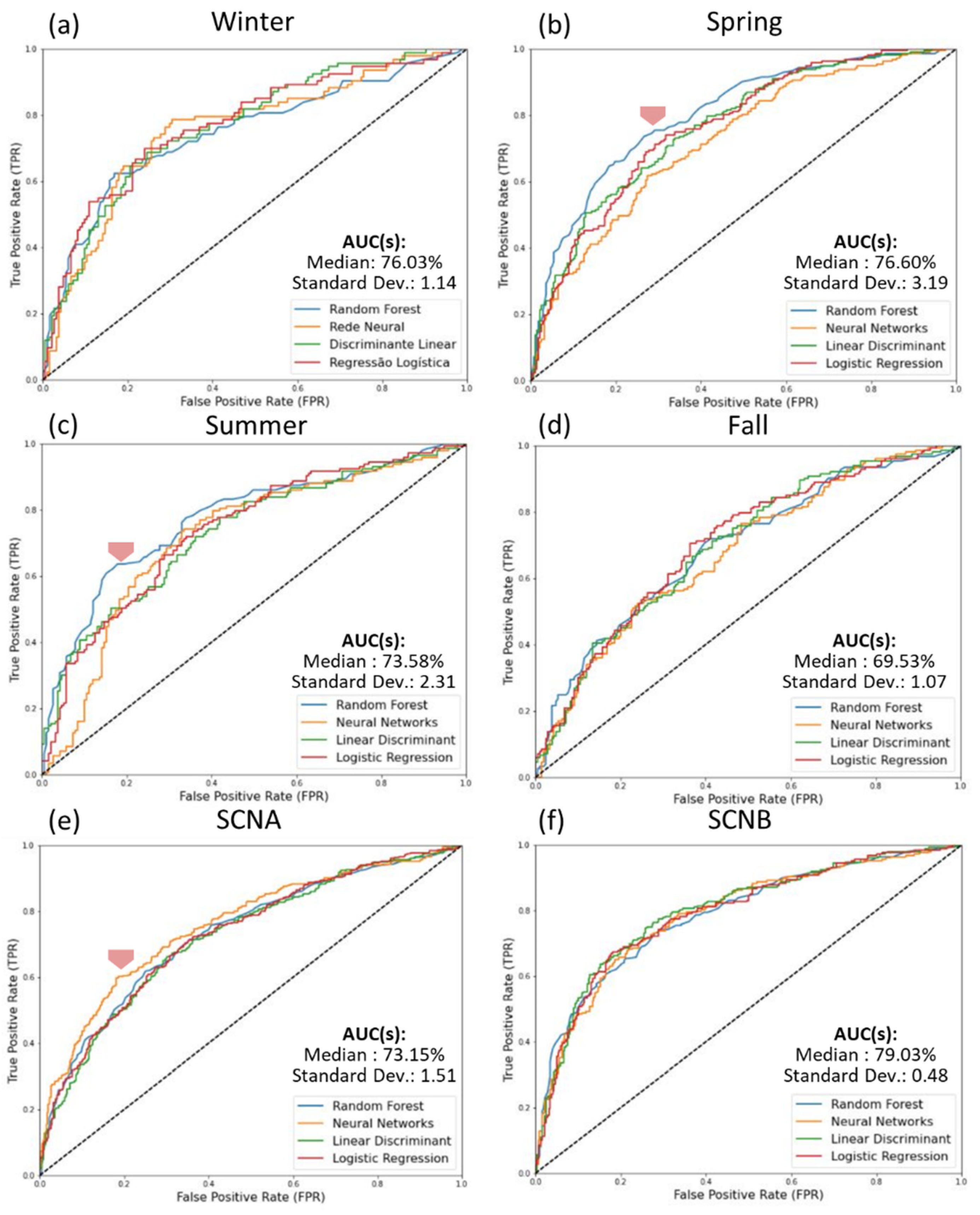
3.2.1. Seasonality Effects on the Classification Model Accuracy

As mentioned previously, many factors can affect the detectability of oil slicks at the sea surface, such as the SAR system configuration, meteo-oceanographic conditions, and the physicochemical properties of different oil types. The available database indicates in which season each oil slick was detected, giving indirect clues about the wind behavior. This information allows for evaluating the benefits of building and fitting SCMs considering seasonality effects, as the GoM presents significant variations in terms of wind intensity and direction throughout the year.

To accomplish this objective, five scenarios were investigated (Table 2: 1–5), considering the following: (a) All seasons together (All); (b) Winter; (c) Spring; (d) Summer; (c) Fall. Table 1 indicates that, even when the oil samples were divided per season, the classes remained relatively balanced, given (a) Winter (1130: 23), (b) Spring (1205: 24), (c) Summer (921: 19), and; (e) Fall (1660: 34). The goal was to discover the best seasons in which to distinguish seeps from spills, seeking the best algorithms and parameters to optimize the accuracy of each searched model. The maximum prediction accuracies obtained using the four ML algorithms are available in

Table 5. (a) Maximum accuracies and (b) median accuracies for all datasets and for each season, indicating the performances of the algorithms RF, ANN, LDA, and LR.

(a) Maximum Accuracies						(b) Median Accuracies
	All	Winter	Spring	Summer	Fall		All	Winter	Spring	Summer	Fall
RF	73.15	80.51	77.76	73.82	72.93	RF	71.53	74.91	75.80	70.80	68.65
ANN	73.02	77.98	75.15	72.65	73.48	ANN	70.04	75.45	71.99	69.77	67.82
LDA	72.07	78.34	75.35	72.94	73.20	LDA	70.14	74.55	72.99	67.26	68.79
LR	72.00	78.34	73.75	71.76	75.14	LR	70.24	75.27	71.39	67.11	68.51

a, and the median accuracies are available in Table 5b.

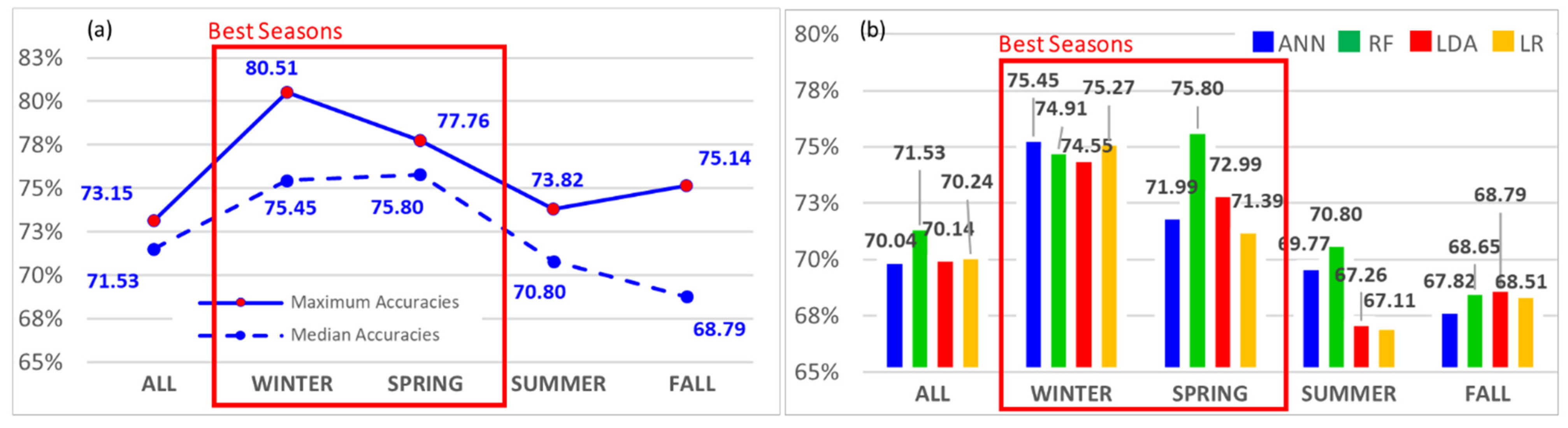
The graph in Figure 6a compares the maximum and median accuracies achieved by the prediction models considering the seasonality effects. Figure 6b provides the median accuracies for all tested ML algorithms, plotting the average and maximum trends as a reference.

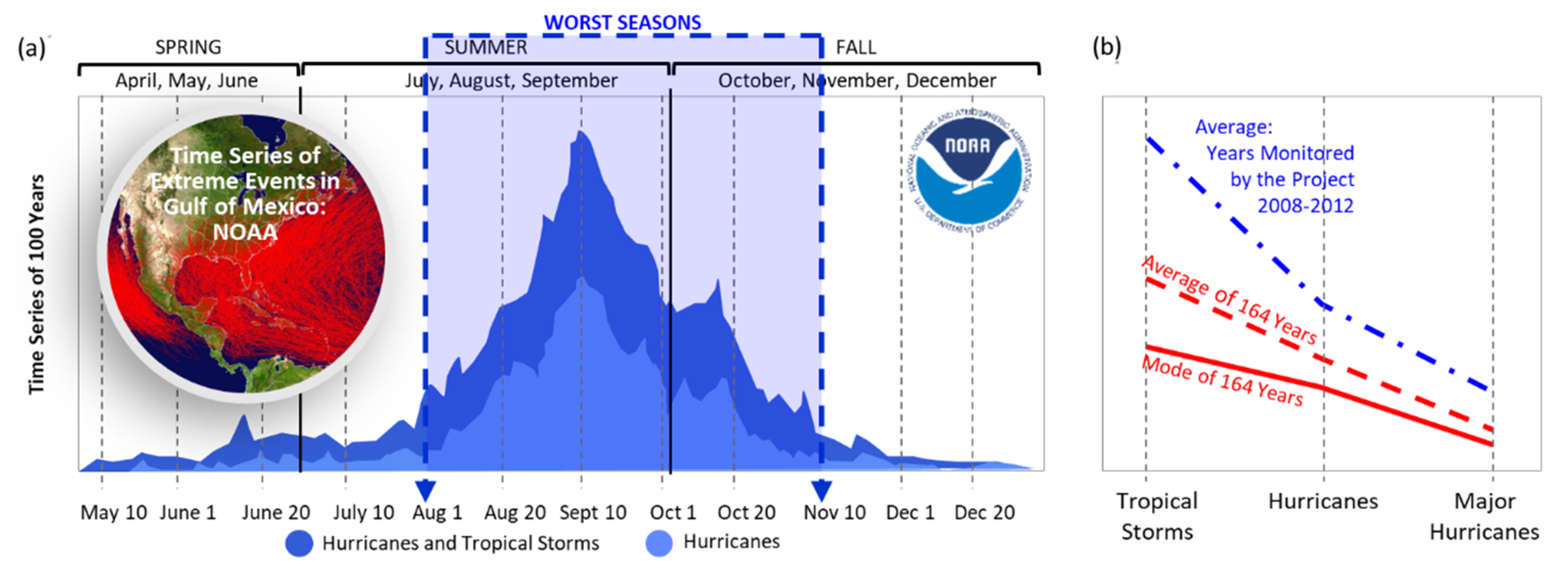
The highest accuracies were obtained during the winter (Max: 80.51; Median: 75.45) and spring (Max: 77.76; Median: 75.80), reaching the worst predictions during the summer (Max: 73.82; Median: 70.80) and fall (Max: 75.14; Median: 68.79). Result consistency was evidenced by a historical database containing more than 100 years of hurricane and tropical storm records (Figure 7a: adapted from https://www.nhc.noaa.gov/climo/ (accessed on 1 May 2020)) in the Atlantic (Atlantic Ocean, Caribbean Sea, and Gulf of Mexico). This database provided by the National Oceanic and Atmospheric Administration (NOAA) [34] shows that the months with the highest incidence of extreme weather events (August, September, and October) coincide with the worst seasons indicated by the prediction models. The occurrence of high-intensity winds during the summer and fall certainly contributed to the worst performance of these models in distinguishing natural from anthropic oil slicks.

Precisely in the years of the project (2008–2012), the time series evidenced a higher incidence of extreme weather events (Figure 7b, blue dashed line), notably with major hurricanes above the NOAA’s average, reinforcing the above conclusions.

Extreme events generate high-intensity winds that increase the heights of the waves and the strength of the gravity currents. These extreme conditions tend to damage pipelines, causing oil spills. Additionally, accumulated damage to oil rigs and vessels, as well as to several other critical facilities in petroleum fields, may indirectly produce oil spills during these events or later. Coincidentally, exactly in the years with the highest incidence of extreme weather events (2010, 2011, 2012), the number of spills was significantly higher than the occurrence of seeps (

Table 6. Number of seeps and spills during the five years of the project.

	Oil Slicks Detected Per Year
Number of Slicks	2008	2009	2010	2011	2012
Seeps	350	319	293	566	493
Spills	328	436	528	769	834
Total	678	755	821	1335	1327
N° of Events	27	14	36	30	31

). Investigating the relationship between the spills and increasing extreme events is an important topic for future research, considering the environmental and socio-economic impacts that oil pollution may have on local ecosystems.

Regarding ML algorithms (Figure 6b), RF showed the highest median accuracies, remaining above average for almost all seasons. It is interesting to note that the maximum accuracy achieved using the complete dataset (73.15) was surpassed during the best (Winter: 80.51) and the worst scenarios (Summer: 73.82).

3.2.2. Effect of the RADARSAT-2 Beam Modes on the Classification Model Accuracy

Since oil slick detectability is also limited by satellite configurations, an analysis regarding the effect of RADARSAT-2 beam modes over OSS predictions is recommended.

Aiming to discover the best SAR configuration, the same 12 features and ML algorithms were used to investigate four scenarios (Table 2, 1, 6–8) as follows: (a) All beam modes together (ALL: W1, W2, SCNA, and SCNB); (b) only the SCN modes (SCN: SCNA and SCNB); (c) SCNA; (d) SCNB. The properties of each beam mode and the respective number of oil slicks detected per beam are available in Table 2.

The Wide modes were not individually evaluated, since they represent only 7% of the oil slicks registered in the database. This poor sample representation by the Wide modes would provide neither robust nor statistically significant results to be evaluated. To avoid an imbalance of classes, the effect of SCN beam modes was solely considered in the analysis. The maximum prediction accuracies obtained are available in

Table 7. (a) Maximum accuracies and (b) median accuracies for all combinations of beam modes, showing the performance of the algorithms RF, ANN, LDA, and LR.

(a) Maximum Accuracies					(b) Median Accuracies
	All	SCN	SCNA	SCNB		All	SCN	SCNA	SCNB
RF	73.15	71.95	74.59	80.00	RF	71.53	71.13	71.65	77.11
ANN	73.02	71.95	73.47	78.77	ANN	70.04	70.29	68.59	76.67
LDA	72.07	70.93	72.59	78.60	LDA	70.14	70.10	69.46	76.58
LR	72.00	70.34	72.34	78.42	LR	70.24	69.96	68.72	76.67

a, and the median accuracies are available in Table 7b.

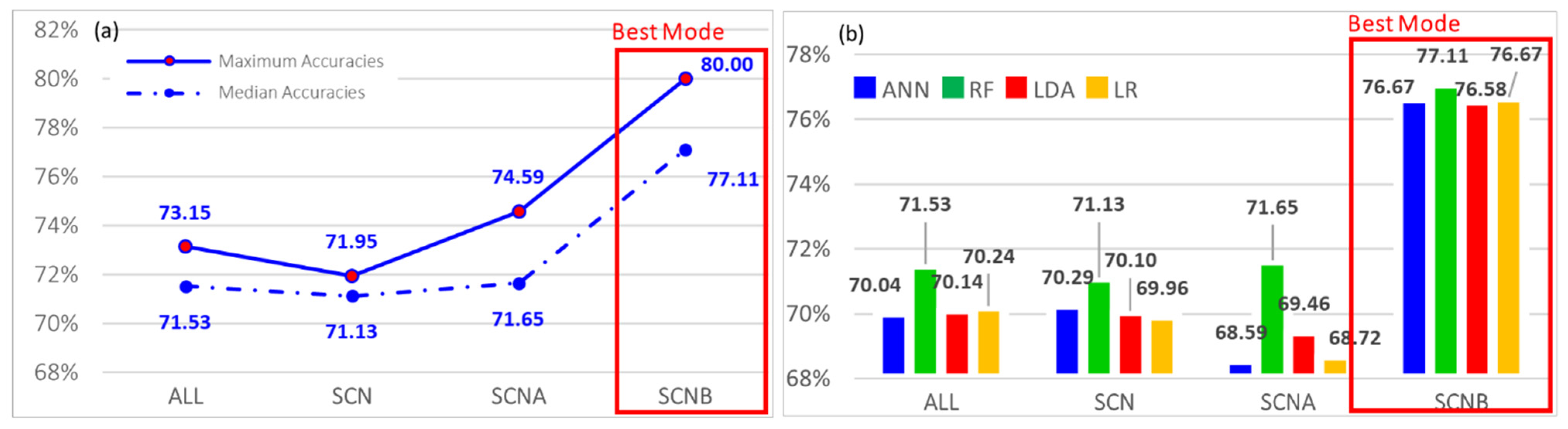
The graph in Figure 8a compares the maximum and the median accuracies achieved by CM considering all beam modes, SCN modes, SCNA, and SCNB. Figure 8b provides the median accuracies for all tested ML algorithms, plotting the average as a reference.

It is interesting to mention that the exclusion of the Wide modes slightly decreased the classification model maximum accuracies, keeping a similar median accuracy (Figure 8a). This indicates that even though in a smaller proportion within the database, the Wide modes may have been positively contributing to OSS identification, probably because of the higher spatial resolution of these modes (26 m) when compared to SCNA and SCNB (50 m). The higher the spatial resolution, the higher the mode’s ability to detect small dark spots, as well as to better delineate the shape and the border of the larger oil slicks.

Another important conclusion can be seen in the graph available in Figure 8a, which indicates that for both modes, SCNA and SCNB, the maximum accuracies improved from 73.15, considering all modes together, to 74.59 with only SCNA, achieving a detectability value of 80 using the SCNB mode. The importance of the SCNB mode is enhanced when examining the median accuracies (Figure 8a, dashed line). This graph demonstrates that the contribution of the SCNB mode to improving CMs is significantly higher (77.11) than that of SCNA (71.65). SCNA showed median accuracies (71.65) similar to those obtained by all modes (71.53) and SCN modes together (71.13).

Thus, SCMs designed for SCNB improved OSS prediction, providing an increment of about 8%, in terms of median accuracies. The higher performances were obtained using the RF algorithm, presenting above average median accuracies for all tested cases (Figure 8b). Particularly for the SCNB mode, all tested ML algorithms showed similar or higher performances, reinforcing the conclusion that SCNB presented better potential to distinguish seeps from spills.

The obtained results are consistent with the concepts regarding the detectability of the sea surface scattering mechanisms using SAR instruments. As mentioned previously, it is well known that SAR viewing geometry and instrument noise floor (NESZ) can affect target detection [12,36,37,38,39].

In this case study, both RADARSAT-2 beam modes, SCNA and SCNB, covered the range of incidence angles recommended by oil slick detection (20° ≤ ϴ_i ≤ 45°), with the same swath width. However, SCNB comprises higher incidence angles (31° ≤ ϴ_i ≤ 47°) with a higher inclined geometry, starting the scene acquisition 11^o above SCNA (20° ≤ ϴ_i ≤ 39°). These characteristics may have enhanced the contrast between the dark spots and the surrounding ocean in the near range.

Moreover, conceptual beam modes like SCNA and SCNB are a multiplexing of different physical beams [38]; consequently, their NESZ is an integration of the noise floor provided by each single mode (

Table 8. Conceptual and real beam modes with the incidence angles, and the maximum and minimum noise floor (NESZ) for SCNA and SCNB.

Beams		Incidence Angles	NESZ (dB)
Conceptual	Real		Maximum	Minimum
SCNA	W1+W2	20–39°	−24.50	−30.00
SCNB	W2+S5+S6	31–47°	−27.00	−30.75

). SCNA merges the geometric and the noise properties of two physical beams, Wide 1 (W1) and Wide 2 (W2), while SCNB merges three different beams, Wide 2 (W2), Standard 5 (S5), and Standard 6 (S6) [38]. Table 8 synthesizes the NESZ in dB, indicating that the maximum and the minimum noise levels are lower for SCNB, remaining 2.5 dB below SCNA.

Therefore, differences in terms of viewing geometry in the near range added to lower noise floor levels, very likely contributed to a better detectability provided by the SCNB mode, probably improving the contrast between the dark spots and the surrounding ocean.

Moreover, since the information about the beam modes can also be depicted per seasonality, a deeper analysis was done considering the synergy effect among them in 12 scenarios (Table 2, 9–20). SCN was not affected after being divided by seasons (Table 2, Scenarios 9–12), thus keeping the previously observed tendency.

The synergy effect between the beam modes and seasonality is perceptible in terms of accuracies for SCNA and SCNB. After dividing SCNA by season (Table 2, Scenarios 13–16), the maximum median accuracy increases from 71.65 to 82.25 during the winter. The same effect occurs for the SCNB mode. Without considering the seasons, the maximum median accuracy is 77.10; after splitting by seasons (Table 2, Scenarios 17–20), it reaches 83.05 during the winter.

Assessing the performances of the algorithms for SCNA, RF kept the best accuracies always above the average, before and after the division by seasons. For SCNB, the behavior of the algorithms was different after splitting, showing that LDA and LR responded better than RF. These results are important to demonstrate the potential of specific models to improve classification results.

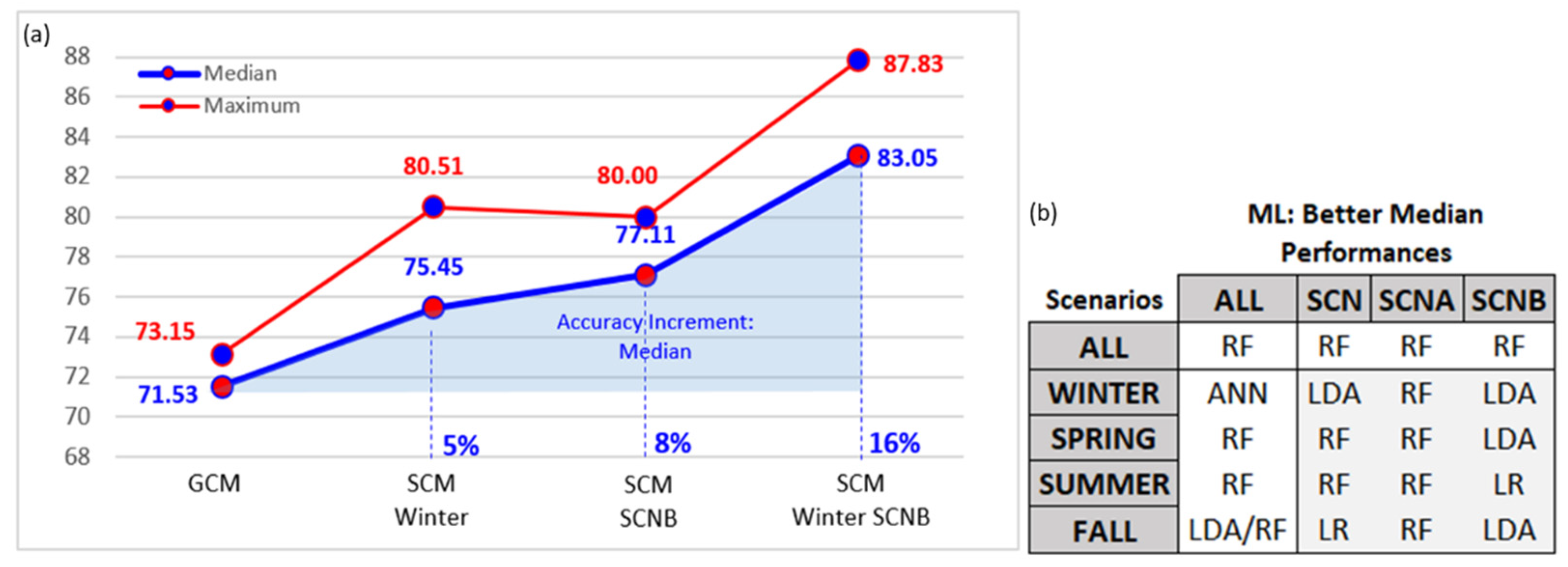
Figure 9a synthesizes the landmarks achieved by classification models in terms of performance. It shows the best maximum accuracies (red line), median accuracies (blue line), and the total increments in terms of median performances, considering (i) the global model (GCM); (ii) the better season (SCM: Winter); (iii) the better beam mode (SCM: SCNB); (iv) the synergy between the best beam mode and season (SCM: SCNB/Winter).

The landmarks evolution shows the potential of optimized models (SCM) to significantly improve the prediction accuracies, which in previous studies, did not surpass a median accuracy of 70 [5,26,27,28]. The seasonality effect provoked an increment of 5% in terms of median accuracy over the best season (winter). SCNB provided a median increment of 8%. Finally, the best scenario showed a median increment of around 16%, accomplishing a maximum accuracy of 87.83 and distinguishing natural from anthropic oils (SCNB/Winter).

Analyzing the best median performances obtained by the tested ML algorithms, the non-parametric RF was the most robust in distinguishing seeps from spills in the GoM. RF delivered the best predictions in 81% of the scenarios (13), offering the best potential for distinguishing natural from anthropic oil slicks (Figure 9b). Regarding satellite configurations, the best predictions were obtained employing RF in all combinations of beam modes (Figure 9b). RF offered the best performances for spring, summer, and fall, while ANN had the best only for winter. RF robustness for oil slick detection has also been evidenced by different authors [47,52,63,64,65]. However, the parametric algorithms LDA and LR offered better performances mainly after the synergy between the beam modes and seasons. Five out of 20 scenarios responded well using LDA and two responded well using LR (Figure 9b). It is likely that the lower number of training samples available for these scenarios justifies the results, as parametric methods require a smaller number of samples for training [41,42,43,44].

4. Discussion

As previously mentioned, distinguishing seeps from spills is a crucial task for the oil and gas sector. The automatic identification of OSS is a trustworthy way to provide ancillary information for guiding environmental and exploratory studies. The identification of OSS as natural may protect the oil industry against penalties for events in which there was no human intervention. Moreover, the oil seep clusters, detected under a machine learning approach, can be integrated with geological, geochemical, and geophysical information, enriching the studies for discovering new exploratory frontiers.

From this standpoint, it is desirable to evaluate the misclassification of a spill as a seep (false positive rate: FPR) and of a true oil seep as a spill (false negative rate: FNR). On this basis, the area under the receiver operating characteristic (ROC) curve (AUC) was estimated using cross-validation to provide a more detailed assessment of the classifiers’ sensitivity, setting the oil seep class as the true positive (TP).

Table 9. (a) Median accuracies and standard deviations for the AUC(s) from the SCM, and (b) the median accuracies for the global CM.

(a) Area under the ROC Curve (AUC): Sensitivity for Oil Seeps
Algorithm	All	Winter	Spring	Summer	Fall	SCNA	SCNB
RF	73.91	74.65	80.24	77.30	69.39	73.30	78.90
ANN	74.74	75.41	72.43	71.86	67.90	75.77	78.94
LDA	76.00	76.64	76.64	73.25	69.66	72.30	79.92
LR	75.90	77.15	76.55	73.90	70.46	73.00	79.11
Median	75.32	76.03	76.60	73.58	69.53	73.15	79.03
σ	1.00	1.14	3.19	2.31	1.07	1.51	0.48
Better AG	LDA	LR	RF	RF	LR	ANN	LDA
(b) GLOBAL ACCURACY (GA)
	All	Winter	Spring	Summer	Fall	SCNA	SCNB
Median	71.53	75.45	75.80	70.80	68.79	71.65	77.11
Better AG	RF	ANN	RF	RF	LDA	RF	RF

presents a comparison of the calculated AUC for each tested algorithm, considering all data, seasonality, and satellite beam modes (Table 9a), with median global accuracies for the same datasets without considering errors (Table 9b).

Detailing the results, the AUC medians (Table 9a) are higher than those of global accuracies (Table 9b) in all scenarios. Even considering the seeps correctly classified (true positive rate: TPR) by the classification errors (FPR), the global trend verified for the four seasons is maintained by AUC(s), confirming winter and spring as the best seasons, and summer and fall as the worst for oil seep identification. In the same way, the trend observed for global accuracies is also preserved for satellite configurations, keeping the highest AUC(s) associated with the SCNB mode. AUC curves considering the seeps correctly classified (TPR) by the spills misclassified as seeps (FPR) are shown in Figure 10. The higher the AUC, the better the potential of the classification model for identifying oil slicks coming from natural sources.

Considering all the studied scenarios utilizing the four ML algorithms (Figure 10), interesting conclusions can be drawn by analyzing the geometric patterns of the curves together with the median values of the AUC(s) and their respective standard deviations (ơ).

For seasonality, the highest standard deviations occurred during spring and summer (

Table 10. K-fold cross-validation, indicating the accuracy intervals obtained per algorithm for global and specific models (minimum and maximum accuracies).

K-Fold Cross-Validation = 5: Accuracy Interval (Minimum and Maximum Accuracies)
	RF	ANN	LDA	LR
All	[61.54~75.41%]	[63.07~73.87%]	[68.84~71.50%]	[64.38~76.64%]
Winter	[67.80~81.29%]	[65.14~80.32%]	[66.47~83.53%]	[65.95~83.14%]
Spring	[64.01~78.84%]	[65.88~72.90%]	[59.33~75.37%]	[66.62~74.19%]
Summer	[61.01~82.27%]	[55.30~73.06%]	[63.53~72.83%]	[57.36~79.01%]
Fall	[45.35~76.87%]	[57.34~68.68%]	[58.30~73.20%]	[61.11~75.01%]
SCNA	[67.83~69.67%]	[64.71~77.79%]	[62.66~70.68%]	[65.08~72.42%]
SCNB	[66.91~82.22%]	[65.50~80.12%]	[65.25~85.63%]	[63.62~82.00%]

a), suggesting that the ML algorithm made a difference in obtaining the best performances. In these seasons, RF achieved higher AUC(s) (blue lines in Figure 10b,c), confirming the same algorithm highlighted for the global accuracies (Table 10b). The winter and fall seasons presented more stable performances among the ML algorithms (Figure 10a,d), showing lower standard deviations among the AUC(s).

A lower standard deviation (Table 10a) among the AUC(s) was obtained for the SCNB mode. A similar behavior among its curves reflects it (Figure 10f), reinforcing SCNB as the best beam mode for oil seep identification, regardless of the employed algorithm. The results centered in the oil seep class reinforce the importance and benefit of investigating and selecting the optimal classifiers and configurations for OSS identification.

Table 10 summarizes the accuracy intervals calculated by the k-fold cross-validation applied to the global and specific models, considering all tested algorithms. The distance between the minimum and maximum accuracies, for each season and SCN mode, indicates no over-fitting for the developed classification models.

5. Conclusions and Outlook

Understanding the relationships among features, algorithms, and parameters is crucial for developing efficient rules to be implemented in expert systems aiming to fit classification models in order to run under favorable and unfavorable conditions. In this framework, feature selection is strategic from an operational point of view, as it minimizes the time required for attribute calculation, data pre-processing, and data analysis. A detailed EDA successfully reduced the data dimensionality, selecting 12 features and preserving its representativeness without compromising classification accuracies.

Seasonality causes a significant impact on oil slick source (OSS) identification. The best seasons to acquire SAR data in order to distinguish seeps from spills in the Gulf of Mexico (GoM) are winter and spring. The predictions evidenced the sensitivity and the potential offered by the models’ specifications in terms of features, algorithms, and parameters selection, consolidating a robust approach to improve classification accuracy. Coherently, the worst seasons, summer and fall, coincide with the hurricane season in the GoM, where high-intensity winds really hamper oil slick detection using SAR instruments. When analyzing the sensitivity of the models for oil seep class detection, this tendency was confirmed by the areas under the ROC curve (AUC). Although some algorithms provided a better response in specific scenarios, RF appeared to be the most robust one to distinguish seeps from spills for global and specific classification models.

Oil slick detectability on the sea surface is also affected by satellite configurations. In fact, from the analyzed beam modes, SCNB offered the best potential when considering both the global accuracies and AUC(s). All designed models were trained and tested with attributes extracted from Radarsat-2 images in C Band. However, different beam modes affected the prediction performances. Thus, although the developed models can be applied to other airborne or orbital SAR sensors in C Band, carrying out training with samples from different satellites, spatial resolutions, and incidence angle ranges is recommended.

Hence, there is no perfect algorithm, since their performances are case-specific and can be affected by dataset quality, geographic region, environmental factors, and satellite configuration, as well as by the number of samples available [30,31,41,69].

The adopted ML approach is powerful as well as innovative and demonstrates how these specific models (SCMs) can operate under different real-world conditions. These added-value products are strategic for operational activities, helping remote sensing specialists to select the best SAR products and seasons for new acquisitions in exploratory projects. However, only when archived data are available is it possible to set the proper algorithms and parameters according to season and beam mode, which optimizes the detectability even under unfavorable weather conditions.

The gains in terms of accuracy provided by well-fitted models minimize the confusion between natural and anthropic oil slicks, contributing to three important applications—(i) providing ancillary information for supporting environmental studies; (ii) securing the oil industry against penalties for events in which there was no human intervention; (iii) reducing geologic risks related to oil generation and migration in offshore exploration frontiers.

Therefore, the particularities observed for each SCM have opened new fronts for more in-depth research on the feasibility and applicability of these models as a way to increase accuracy. For instance, a more precise investigation into how different incidence angles (θi) improve OSS detectability is recommended. In a wider domain, the global model generalization capacity should be assessed in future initiatives over different geographic regions, including the contribution of new features and algorithms to OSS prediction.