Article

A Robust InSAR Phase Unwrapping Method via Phase Gradient Estimation Network

School of Information and Communication Engineering, University of Electronic Science and Technology of China, Chengdu 611731, China
*
Author to whom correspondence should be addressed.
Remote Sens. 2021, 13(22), 4564; https://doi.org/10.3390/rs13224564
Submission received: 1 September 2021 / Revised: 27 October 2021 / Accepted: 9 November 2021 / Published: 13 November 2021
(This article belongs to the Special Issue Synthetic Aperture Radar (SAR) Meets Deep Learning)

Abstract

:
Phase unwrapping is a critical step in synthetic aperture radar interferometry (InSAR) data processing chains. In almost all phase unwrapping methods, estimating the phase gradient according to the phase continuity assumption (PGE-PCA) is an essential step. The phase continuity assumption is not always satisfied due to the presence of noise and abrupt terrain changes; therefore, it is difficult to get the correct phase gradient. In this paper, we propose a robust least squares phase unwrapping method that works via a phase gradient estimation network based on the encoder–decoder architecture (PGENet) for InSAR. In this method, from a large number of wrapped phase images with topography features and different levels of noise, the deep convolutional neural network can learn global phase features and the phase gradient between adjacent pixels, so a more accurate and robust phase gradient can be predicted than that obtained by PGE-PCA. To get the phase unwrapping result, we use the traditional least squares solver to minimize the difference between the gradient obtained by PGENet and the gradient of the unwrapped phase. Experiments on simulated and real InSAR data demonstrated that the proposed method outperforms the other five well-established phase unwrapping methods and is robust to noise.

Graphical Abstract

1. Introduction

Synthetic aperture radar interferometry (InSAR) is playing an increasingly important role in the field of surface deformation monitoring and topographic mapping [1,2,3]. The InSAR system uses two co-registered complex images from different viewing angles to obtain the two-dimensional interferometric phase images. Due to the trigonometric function in the transmitting and receiving models, the obtained interferometric phase is wrapped—that is, its range is in ( π , π ] [4,5]. In order to obtain an accurate elevation measurement of the surveying area, the unwrapped phase must be obtained by adding the correct wrap count to each pixel of the wrapped phase, which is called phase unwrapping. Therefore, in the InSAR data processing pipeline, the measurement accuracy of elevation level is highly correlated with the accuracy of phase unwrapping.
Since phase unwrapping is an ill-posed problem, the phase continuity assumption is usually considered in the process of phase unwrapping: the absolute values of the gradients in the two directions of the unwrapped phase are less than π [6]. Under this assumption, many kinds of phase unwrapping methods have been presented in recent decades, and they can be divided into two categories: path following [5,7,8] and optimization-based methods [9,10,11,12,13,14,15]. A path following method selects the integration path for integrating the estimated phase gradient through the residue distribution or the phase quality map, so as to avoid the local error from being propagated globally. Examples are the branch-cut method [5] and the quality-guided method [7]. An optimization-based method minimizes the difference between the estimated gradient and the unwrapping phase gradient through the objective function to obtain the optimal unwrapped phase. Examples are the least squares (LS) method [13] and the statistical-cost, network-flow algorithm for phase unwrapping (SNAPHU) method [15], and phase unwrapping max-flow/min-cut algorithm (PUMA) [10]. Both types of method need to obtain the estimated value of the phase gradient through the phase continuity assumption before unwrapping. Due to the presence of noise and abrupt terrain changes, the phase continuity assumption is not always satisfied—that is, the unwrapped phase may jump above π , which may cause local errors in the unwrapping process. This local error may produce a global error along the integration path, so the estimated phase gradient information will directly affect the final unwrapping accuracy. Therefore, it is a valuable aim to seek a more accurate estimation method of phase gradient information instead of directly relying on the traditional estimation method based on the phase continuity assumption.
In recent years, the deep learning-based phase unwrapping methods have attracted significant interest [16,17,18,19,20,21,22,23,24]. Most of these methods [16,17,18] convert the unwrapping problem into a classification problem of the wrap count, and their effectiveness is verified using optical images. In the field of InSAR, the unwrapping problem becomes more difficult because of two characteristics: the complex wrapped phase caused by topography features and the low coherence coefficient. Therefore, combining traditional phase unwrapping methods with deep learning, instead of relying solely on deep learning, is a promising development trend [19,20,21,22,23]. In [19], a modified fully convolutional network was first applied to classify the wrapped phase into normal pixels and layover residues, which can suppress the error propagation of layover residues during the phase unwrapping process. Additionally, a CNN-based unwrapping method was proposed in [20], which feeds the wrapped phase and coherence map into the network at the same time for training to obtain the wrap count gradient. In this method, the wrap count reconstruction is necessary for obtaining the final unwrapping result. A deep learning-based method combined with the minimum cost flow (MCF) unwrapping model was proposed in [21]. In this method, the phase gradient is discretized to match the MCF unwrapping model and treated as a three-classification deep learning problem, but the number of categories may need to change according to the terrain changes, because the three categories cannot cover all situations. In addition, the ambiguity gradient [23] is taken as ground truth for network training, and the MCF model is used as the postprocessing step for final unwrapped phase reconstruction. However, the MCF unwrapping model is usually very complex computationally and requires numerous computational resources [25].
The LS phase unwrapping method is widely used in practical applications and converges quickly [9,26,27]; therefore, we considered combining it and deep learning to improve the unwrapping accuracy while retaining the advantages of the LS method. In the traditional LS method, estimating the phase gradient according to the phase continuity assumption (PGE-PCA) is an essential step. Recent studies [28,29,30,31,32] have indicated that the encoder–decoder architecture based on deep convolutional neural networks (DCNN) can learn the global features from a large number of input images with different levels of noise or other disturbances, which is useful for obtaining the robust phase gradient from noisy wrapped phase images.
In this paper, we propose a robust LS InSAR phase unwrapping method that works via a phase gradient estimation network (PGENet-LS). In this method, we transform the phase gradient estimation into a regression problem and design a phase gradient estimation network based on the encoder–decoder architecture (PGENet) for InSAR. From lots of wrapped phase images with topography features and different levels of noise, PGENet can extract global high-level phase features and recognize the phase gradient between adjacent pixels, so the more accurate and robust phase gradient can be estimated by PGENet than that obtained by PGE-PCA. Finally, the phase unwrapping result is obtained by using the least squares solver to minimize the difference between the gradient obtained by PGENet and the gradient of the unwrapped phase. The phase gradient estimated by PGENet is used to replace the PGE-PCA in the traditional LS unwrapping method. As the accuracy of the phase gradient estimated by PGENet is significantly higher and more robust than that of the phase gradient estimated by PGE-PCA, the proposed method has higher accuracy than the traditional LS phase unwrapping method. A series of experimental results of simulated wrapped phase and real InSAR data demonstrate that the proposed method outperforms the other five well-established phase unwrapping methods and is robust to noise.
This paper is organized as follows. Section 2 introduces the principles of phase unwrapping, problem analysis, PGENet, and the proposed method. In Section 3, the data generation method, loss function, performance evaluation index, and experiment settings are described. In Section 4, a series of experimental results using simulated and real InSAR data are presented. Section 5 and Section 6 present the discussion and conclusions of the paper, respectively.

2. PGENet-LS Phase Unwrapping Method

In this section, we first introduce the principle of phase unwrapping and how to use deep neural networks instead of PGE-PCA to estimate the phase gradient. Then we describe the detailed structure of PGENet, and finally introduce the processing flow of the PGENet-LS phase unwrapping method.

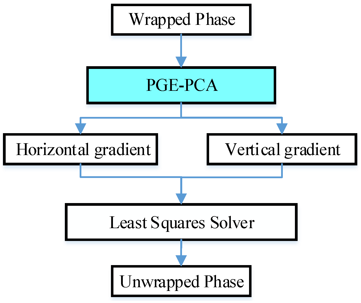
2.1. Principle of Phase Unwrapping

The wrapped phase is distributed in ( π , π ] containing the ambiguities of integral multiples of 2 π . For an image pixel point ( i , j ) , the relationship between the wrapped phase ϕ i , j and the unwrapped phase φ i , j can be expressed as
φ i , j = ϕ i , j + 2 π k i , j
where k i , j is a sequence of integers, which is called the wrap count. When k i , j is known, the unwrapped phase can be recovered from the wrapped phase. However, a unique solution k i , j cannot be obtained because there are two unknowns in (1). Therefore, in the traditional phase unwrapping method, the phase continuity assumption is used to ensure the uniqueness of the phase unwrapping result. Under this assumption, the LS phase unwrapping method can be divided into the following two steps: phase gradient estimation and implementation of the least squares solver. The flowchart is shown in Figure 1.
Step 1: According to the phase continuity assumption, for the two-dimensional phase unwrapping issue, the horizontal gradient and vertical phase gradient can be estimated by
Δ i , j x = ϕ i , j + 1 ϕ i , j , π ϕ i , j + 1 ϕ i , j π ϕ i , j + 1 ϕ i , j 2 π , π < ϕ i , j + 1 ϕ i , j 2 π ϕ i , j + 1 ϕ i , j + 2 π , 2 π ϕ i , j + 1 ϕ i , j < π
Δ i , j y = ϕ i + 1 , j ϕ i , j , π ϕ i , j + 1 ϕ i , j π ϕ i + 1 , j ϕ i , j 2 π , π < ϕ i , j + 1 ϕ i , j 2 π ϕ i + 1 , j ϕ i , j + 2 π , 2 π ϕ i , j + 1 ϕ i , j < π
where Δ i , j x and Δ i , j y are the horizontal gradient and vertical gradient, respectively. For brevity, the step is called PGE-PCA.
Step 2: After obtaining the estimated horizontal gradient Δ i , j x and vertical gradient Δ i , j y , the final unwrapping result φ i , j can be calculated according to the least squares solver of (4).
arg min φ i , j i j φ i , j + 1 φ i , j Δ i , j x 2 + i j φ i + 1 , j φ i , j Δ i , j y 2
The meaning of (4) is to minimize the difference between the estimated gradient and the gradient of the unwrapped phase. To obtain the solution of (4), there are mainly two classes of fast algorithms: transformation-based methods [13] and multi-grid methods [12]. We can see that the accuracy of the phase unwrapping result from (4) is directly related to the accuracy of the estimated phase gradient. In other words, if the accuracy of the estimated phase gradient can be improved, we can obtain the more accurate phase unwrapping result.

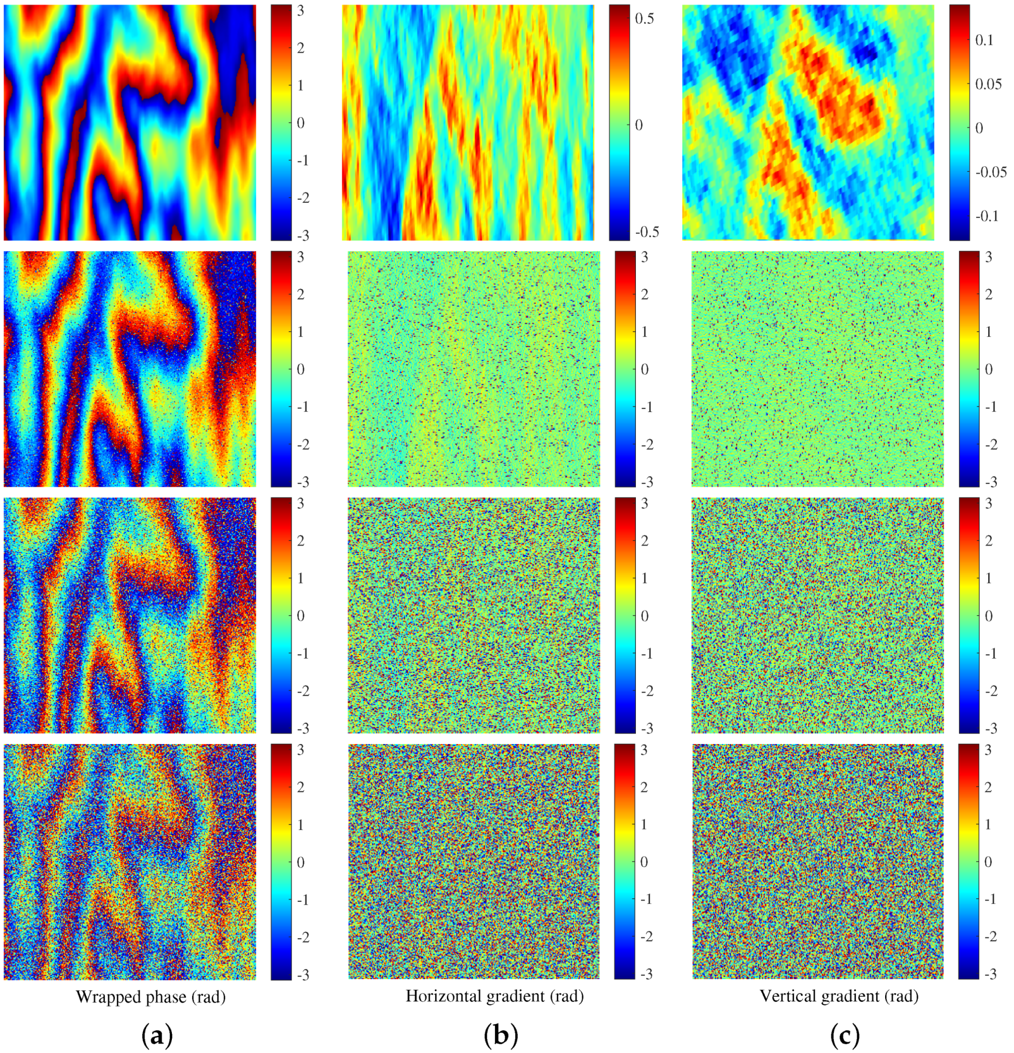
2.2. Problem Analysis
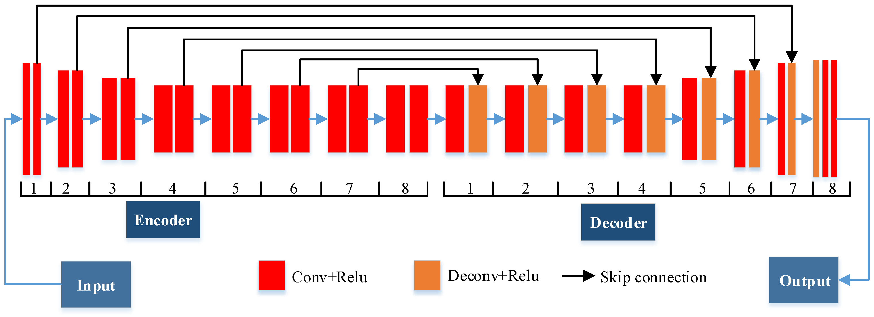
In practical applications, the phase continuity assumption is often not satisfied in every pixel due to the presence of noise and abrupt terrain changes. The noise level can be evaluated by the coherence coefficient, which can be expressed as
ρ = | E { S 1 · S 2 * } E { | S 1 | 2 } · E { | S 2 | 2 } |
where S 1 and S 2 are the co-registered master and slave complex images, respectively; * denotes the complex conjugate; and E { · } denotes the mathematical expectation.
Figure 2 shows the influences of different coherence coefficients on the wrapped phase and the corresponding gradients in the horizontal and vertical directions. Figure 2a shows the wrapped phase with different coherence coefficients, and Figure 2b,c shows the corresponding phase gradients in two directions obtained by (2) and (3), respectively. We can see that in the case of a coherence coefficient of 1 (no noise), the accurate vertical and horizontal phase gradients can be obtained by (2) and (3), but in the presence of noise, the estimated phase gradients in two directions from (2) and (3) are no longer reliable because the gradient information is destroyed by noise. As the coherence coefficient gets lower and lower, the phase gradients in two directions are destroyed more and more severely. From (2) and (3) and Figure 2, we can see that only considering the relationship between adjacent pixels to calculate the gradient is not enough, which means that more or even global phase information may need to be employed. Therefore, in the presence of noise, we use the global phase information in the gradient estimation process for improving the accuracy of phase gradient estimation. That is to say, the gradient estimation of each pixel does not only depend on the adjacent pixels but on the overall wrapped image.
In recent years, the encoder–decoder architecture based on DCNN has been widely used in image processing in the fields of optics, medicine, and SAR [29,30,31,32]. These studies have indicated that the encoder–decoder architecture can learn the global high-level features from input images with different levels of noise or other disturbances. The powerful feature extraction capability is conducive to extract global phase features from the noisy wrapped images to obtain the accurate phase gradient. In addition, according to (2) and (3), it can be seen that the gradient calculation principles in the two directions are the same. Therefore, while the original wrapped phase image and the horizontal gradient image are used as an image pair, the transposed original wrapped phase image and the transposed vertical gradient image of the original wrapped phase image are taken as another equivalent image pair, so that we can get the horizontal and vertical gradient images of the wrapped phase after inputting the original and transposed wrapped phase images to a network, respectively. Based on the above analysis, we designed PGENet based on the encoder–decoder architecture that takes the original or transposed wrapped phase images as inputs and outputs the estimated horizontal or vertical phase gradient images. The deep convolutional neural network can learn global phase features and the phase gradient between adjacent pixels from lots of wrapped phase images with topography features and different coherence coefficients; hence, the accurate and robust horizontal and vertical phase gradient images can be predicted after training.

2.3. PGENet

PGENet is designed based on the encoder–decoder architecture and is mainly composed of two parts: an encoder and a decoder. Its overall structure and the detailed parameters of each layer are shown in Figure 3 and Table 1, respectively. As shown in Figure 3 and Table 1, the encoder part (Encoder) contains eight encoder blocks and converts the input noisy wrapped phase images into more feature maps with smaller sizes, which can enrich the global phase gradient features and reduce memory requirements when adding the number of feature maps. An encoder block is constitutive of two convolution layers (Conv + Relu), and each layer performs two operations, namely, convolution and activation (Relu). After the encoding process, a large number of global phase features are extracted in the feature maps. The decoder part (Decoder) contains eight decoder blocks and gradually recovers the phase gradient from these extracted global phase feature maps. Each decoder block is constitutive of a convolution layer and a deconvolution layer (Deconv + Relu). Each deconvolution layer performs two operations, namely, deconvolution and activation. During the decoding process, a large number of feature maps are gradually merged into larger images until the output image is the same as the input image. At the same time, due to the fusion of global phase features, the accurate phase gradient is extracted.
In the process of constructing the Encoder and Decoder, a deep network structure is formed. The deep architecture of PGENet is used to enrich the level of phase gradient features, which can ensure that the network has sufficient phase gradient estimation capabilities when processing noisy wrapped phase images. While increasing the network depth, the feature maps with the same size between the encoder and decoder are added by skip connections [28]. As shown in Figure 3, the skip connections can transfer the extracted global phase features containing more detailed gradient information to the deconvolution layer of the Decoder and accelerate convergence. Therefore, in the decoder process, the low/mid/high-level global phase gradient features containing more detailed information from the Encoder are compensated and fused in the current phase gradient feature maps. Under the effect of the deep structure and skip connections, PGENet can obtain accurate and robust phase gradient estimation results when inputting images with different noise levels.

2.4. PGENet-LS Phase Unwrapping Method

As shown in Figure 4, in the PGENet-LS phase unwrapping method, the horizontal and vertical gradients are estimated by PGENet first, and then the least squares solver is employed to minimize the difference between the gradients obtained by PGENet and the gradients of the unwrapped phase. Therefore, the processing flow can be divided into the following two steps: phase gradient estimation and unwrapping using the least squares solver.
Step 1: For estimating the phase gradients using PGENet, training and testing are required. PGENet takes the original or transposed wrapped phase images with different coherence coefficients and topography features as input and produces the corresponding horizontal or vertical gradient images. During the training processing, the loss function described in Section 3.2 is selected to update the trainable parameters. During the testing processing, the testing wrapped phase image (simulated or real InSAR data) or its transposed version is fed into the trained PGENet to obtain the estimated horizontal or vertical phase gradient images, respectively.
Step 2: After obtaining the horizontal gradient and vertical gradient estimated by PGENet, all least squares solvers based on phase gradients from (2) and (3) can be used in this step. In this paper, the well-established weighted least squares solver of (6) [26] are selected to get the unwrapping result and can be expressed as
arg min φ i , j i j ω i , j x φ i , j + 1 φ i , j Δ i , j x 2 + i j ω i , j y φ i + 1 , j φ i , j Δ i , j y 2
where w i j x = min w i , j + 1 2 , w i , j 2 , and w i j y = min w i + 1 , j 2 , w i , j 2 . w i j x are the weights defined as the normalized cross-correlation coefficient.

3. Experiments

In this section, the detailed data generation process, loss function, and performance evaluation index are described.

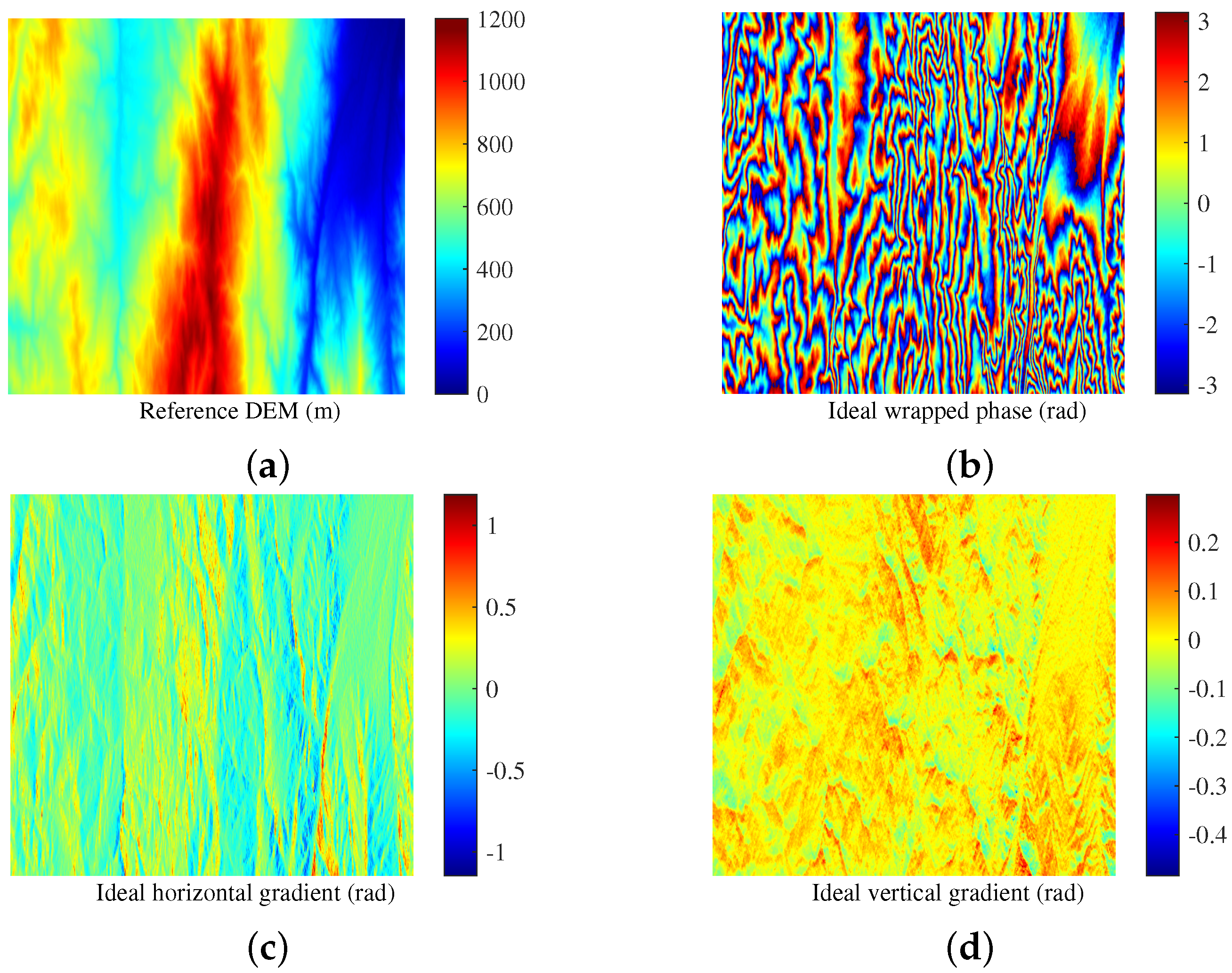
3.1. Data Generation

To make the trained PGENet have a good generalization capability, a large number of labeled images with topography features are needed for training. Therefore, we used a digital elevation model (DEM) to generate wrapped phase images according to the ambiguity height of the real InSAR system [21,33]. After generating the wrapped phase, the corresponding ideal horizontal and vertical phase gradients were obtained according to (2) and (3). In addition, different levels of noise were added to the ideal (no noise) wrapped phase images, and the noise level is expressed by the coherence coefficient in the field of InSAR [2,33]. A lower coherence coefficient means a higher noise level, and in the absence of noise, the coherence coefficient is 1. The wrapped phase images with different coherence coefficients were used to train PGENet, which ensured that the trained PGENet had good robustness to noise.
The details of the generated training data are as follows. Figure 5a shows the DEM (eastern part of Turkey, 2048 × 2048 pixels) used for training in this study. It was from SRTM 1Sec HGT and can be downloaded from the Sentinel Application Platform (SNAP). The reason for choosing this DEM data was that their topographic features are similar to those of the real wrapped phase in the subsequent experiments. In addition, the ambiguity height of the simulated system (92.13 m) was the same as that of the real wrapped phase image in the subsequent experiments. Similar topographic features and the same ambiguity height made the phase gradient features of the training data and the real data as similar as possible. According to the ambiguity height and the DEM, the corresponding ideal wrapped phase and horizontal and vertical phase gradient images are shown in Figure 5b–d. The examples of the noisy wrapped phase images are shown in Figure 6. Ten noisy wrapped phase images were generated for training. Their coherence coefficients were in the range of [ 0.5 , 0.95 ] , and the interval was 0.05. This range of the coherence coefficients can cover most common InSAR data. In order to reduce the memory requirement, the whole wrapped phase images were cut into image patches with the size of 256 × 256 pixels. To augment the training data, 128 pixels were shifted on the columns or rows in each cropping process to ensure 50% overlap of adjacent image patches. Therefore, the total number of horizontal and vertical gradient image patches for training was 4500.
The details of the generated testing data are as follows. Figure 7a shows the reference DEM ( 1024 × 1024 pixels) which was used for testing. The 10 noisy wrapped phase images were generated, and the range of the coherence coefficients was the same as that of the training data. Figure 7b shows an example of a noisy wrapped phase with a coherence coefficient of 0.5, and Figure 7c,d shows the ideal horizontal and vertical phase gradients, respectively. The whole wrapped phase images were cut into image patches of 256 × 256 pixels for testing, and 128 pixels were shifted on the columns or rows in each cropping process to ensure 50% overlap of adjacent image patches. Therefore, the total number of horizontal and vertical gradient image patches for testing was 980, accounting for 22% of the sum of training data and testing data.

3.2. Loss Function

The widely-used mean-square error (MSE) [33] is taken as the loss function to update the training parameters of PGENet. It is calculated according to the ideal phase gradient (ground truth) and the estimated phase gradient image (network output), and can be expressed as
L = i = 1 N Δ i Δ i 2 N
where N is the number of phase gradient image pixels; Δ i and Δ i are the ideal gradient and the gradient estimated by PGENet, respectively.

3.3. Performance Evaluation Index

To fully evaluate the accuracy and robustness of the proposed method, we employed qualitative and quantitative methods to perform the evaluation. Qualitative evaluation refers to performing the unwrapping accuracy judgment based on the observation of the image by the naked eye. Therefore, the original wrapped images and DEM images obtained by the unwrapped phases of six different unwrapping methods are simultaneously presented in this paper. To more comprehensively and objectively evaluate the unwrapping accuracy and robustness, the unwrapping failure rate [19] and root mean square error (RMSE) were adopted for quantitative evaluation.
The unwrapping failure rate can be defined as
UFR = 1 M N i = 1 M j = 1 N d i , j
where d i , j = 1 , if φ i , j φ i , j π 0 , otherwise . φ i , j and φ i , j are the estimated unwrapped phase and ideal unwrapped phase, respectively. M and N are the width and height of the unwrapped phase image, respectively. A smaller UFR value means better unwrapping accuracy to a certain extent in simulated data processing.
For simulated data processing, in addition to the unwrapping failure rate, the RMSE between the estimated unwrapped phase and ideal unwrapped phase was also employed to evaluate the unwrapping accuracy. For real InSAR data processing, due to the ideal unwrapped phase being unknown and the ultimate goal of wrapped phase processing being to obtain elevation, we employed the RMSE between the reference DEM and the DEM obtained by the unwrapped phases of different unwrapping methods to evaluate the unwrapping accuracy [20,23]. The formulaic expression of RMSE is
RMSE = j N i M φ i , j φ i , j 2 M N
where φ i , j is the reference DEM image; φ i , j is the DEM image obtained by the estimated unwrapped phase; M and N are the DEM image width and height, respectively. A small RMSE means that the estimated DEM is close to the reference DEM—that is, the unwrapping accuracy is high.

3.4. General Experiment Settings

We implemented all experiments on a PC with an Intel i7-8700K CPU, a NVIDIA GeForce RTX 2080 GPU, and 64G memory. PGENet was trained for 260 epochs with a batch size of 16 on the TensorFlow platform, and Adam optimizer [34] was selected to accelerate training. The initial learning rate was set to 1 × 10 4 and gradually decayed to 0 exponentially. We chose the early stopping method [35,36] to determine when the network would stop iterating. The trained PGENet was used in the following experiments on simulated and real data.

4. Results

Three experiments were implemented to evaluate the unwrapping accuracy and robustness of the proposed method. In the first experiment, we demonstrated the accuracy of the phase gradient and the robustness of PGENet, and compared PGENet with PGE-PCA. In the second experiment, we evaluated the unwrapping accuracy and robustness of the proposed method on simulated data; and we compared the proposed method with the LS [26], QGPU [7], SNAPHU [14], and PUMA [10] unwrapping methods, and a state-of-the-art deep learning-based method [20]. In the third experiment, the proposed method was compared with the three aforementioned phase unwrapping methods using the real Sentinel-1 InSAR data. For a clear comparison, RMSE was used for performance evaluation in these three experiments.

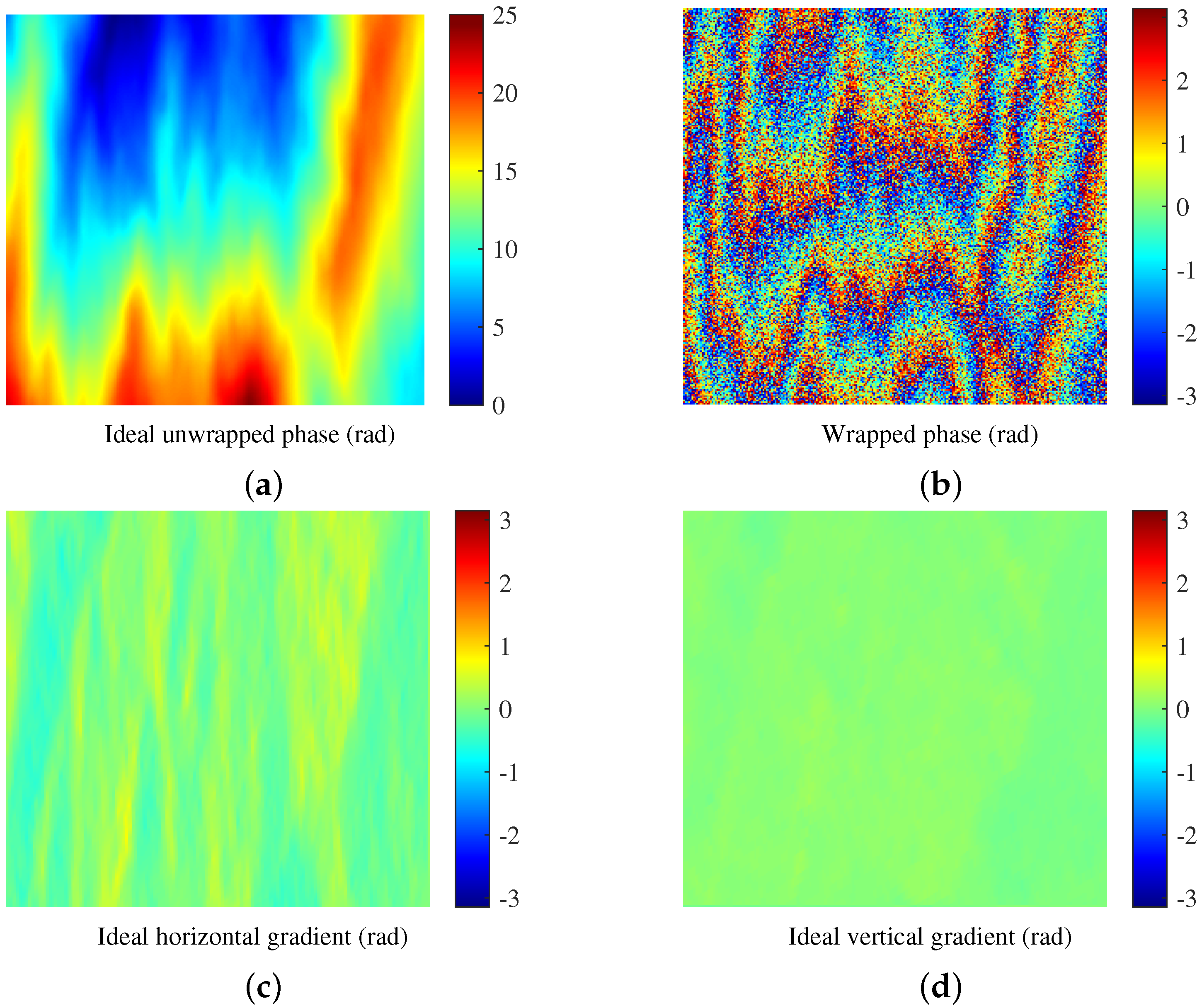
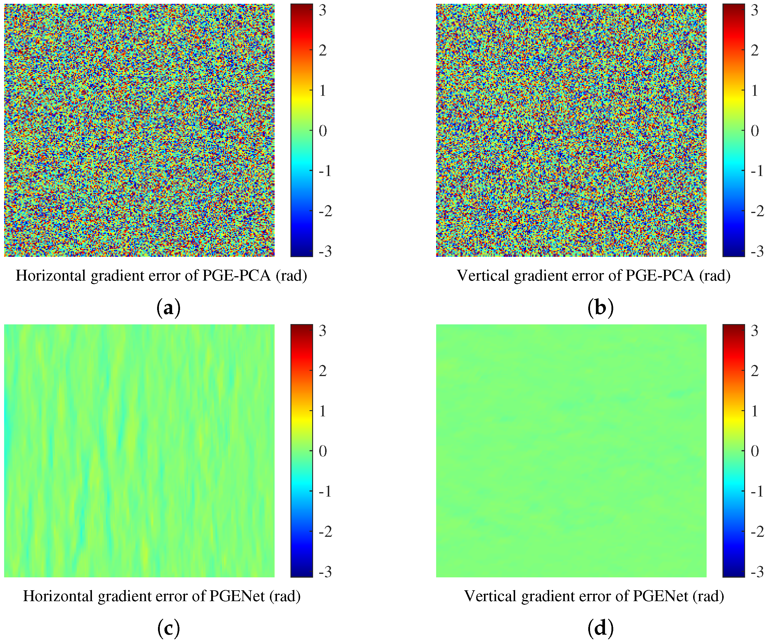
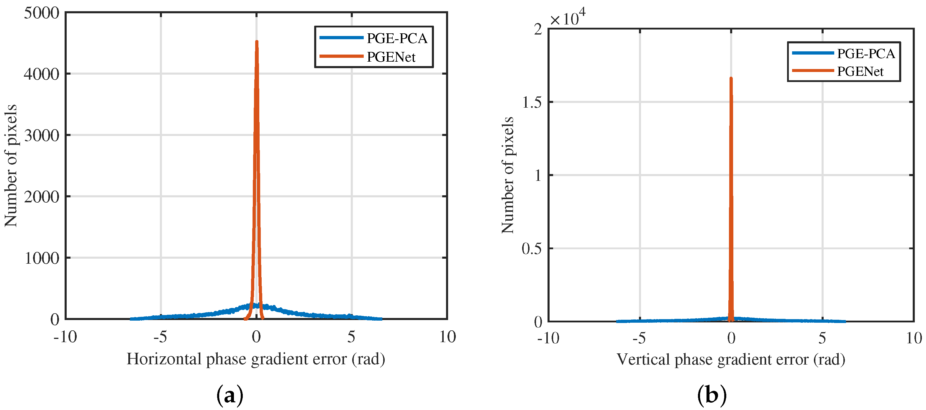
4.1. Performance Evaluation of PGENet

We first selected a testing sample with a coherence coefficient of 0.5 from the testing samples described in Section 3.1 to visually analyze the performance of phase gradient estimation and then evaluate the estimation accuracy of PGENet from the perspective of the phase gradient error. Meanwhile, PGENet was compared with PGE-PCA.
The reference DEM is shown in Figure 8a, and the corresponding wrapped phase image with a coherence coefficient of 0.5 is shown in Figure 8b. Figure 8c,d shows the ideal horizontal and vertical phase gradients, respectively. The horizontal and vertical phase gradients estimated by PGE-PCA are shown in Figure 9a,b, respectively, and the horizontal and vertical phase gradients estimated by PGENet are shown in Figure 9c,d, respectively. The corresponding gradient errors between the results estimated by PGE-PCA and ideal gradients are shown in Figure 10a,b. The corresponding gradient errors between the results estimated by PGENet and ideal gradients are shown in Figure 10c,d. It can been seen that the horizontal and vertical phase gradients obtained by PGENet are very close to the corresponding ideal horizontal and vertical phase gradients because most pixels of its error image are close to zero. In order to better quantify the gradient errors of the two methods, their error histogram curves were fitted according to their gradient error histograms and are shown in Figure 11. The horizontal axis of Figure 11 is the gradient error, and its vertical axis is the corresponding number of pixels of the gradient error image. The histogram curve can clearly shows the error distribution and is convenient for comparing the errors of different methods, so it was also used for subsequent analysis. From Figure 11, regardless of the horizontal gradient error or the vertical gradient error, it can be seen that the error curve of PGENet is more concentrated near zero and sharper than that of PGE-PCA, so the estimation accuracy of PGENet is significantly better than that of PGE-PCA from the perspective of the phase gradient error.

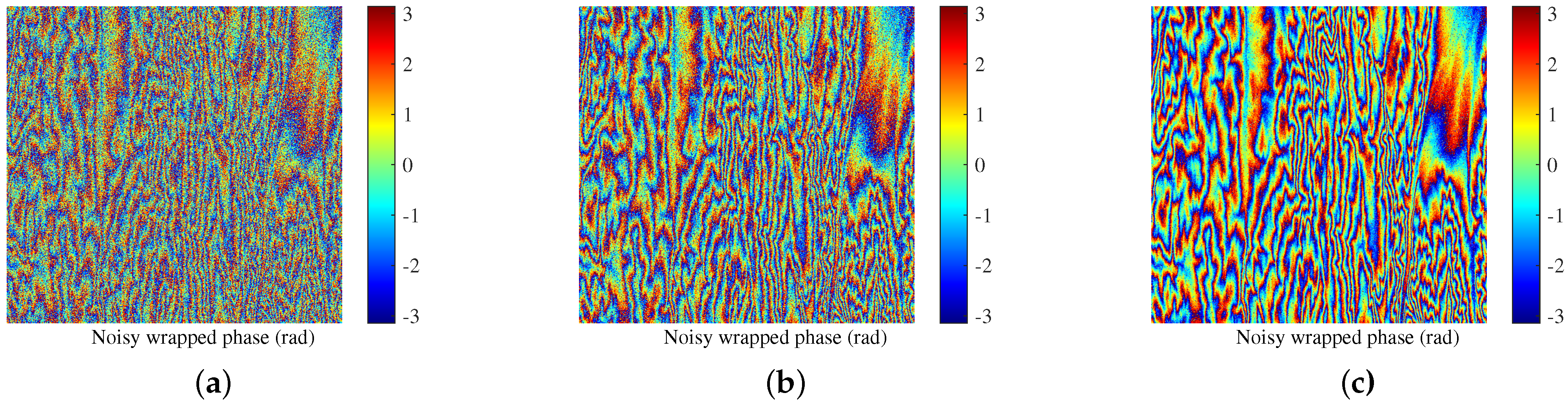
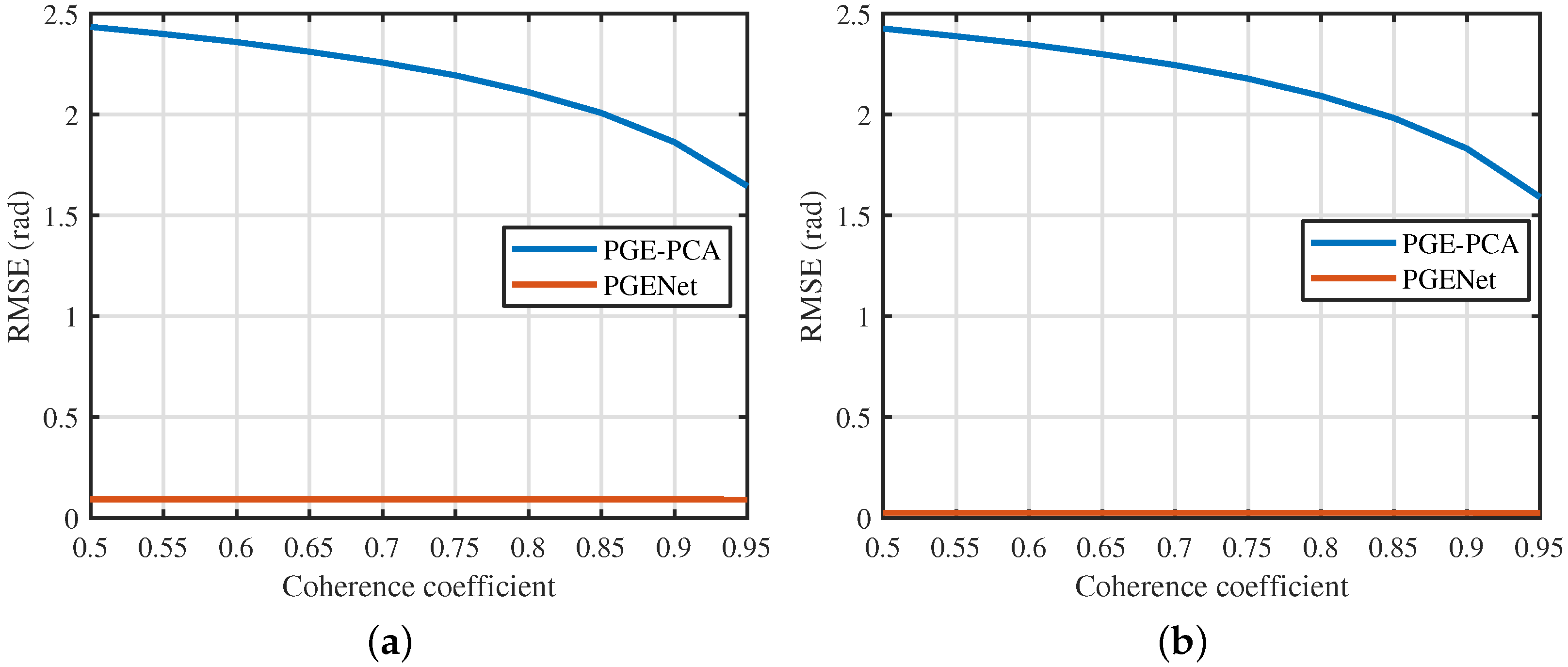
4.2. Robustness Testing of PGENet

As described in Section 3.1, the coherence coefficients of all testing samples ranged from 0.5 to 0.95. For the noise robustness testing, we calculated the mean values of the RMSE of PGENet and PGE-PCA for the testing samples with the same coherence coefficients. The results of the horizontal and vertical phase gradients are shown in Figure 12. Regardless of the horizontal gradient estimation result or the vertical gradient estimation result, we can observe that the RMSE of PGENet is smaller, which means that the accuracy of PGENet was significantly higher than that of PGE-PCA for each considered case. Moreover, the RMSE of PGENet did not change significantly with the changes in the coherence coefficient, which means that PGENet is robust to noise. To evaluate the comprehensive performance in response to different coherence coefficient situations, we calculated the mean values of the RMSE of all testing samples and list the results in Table 2. We can see that PGENet is robust to noise and has higher estimation accuracy than PGE-PCA.

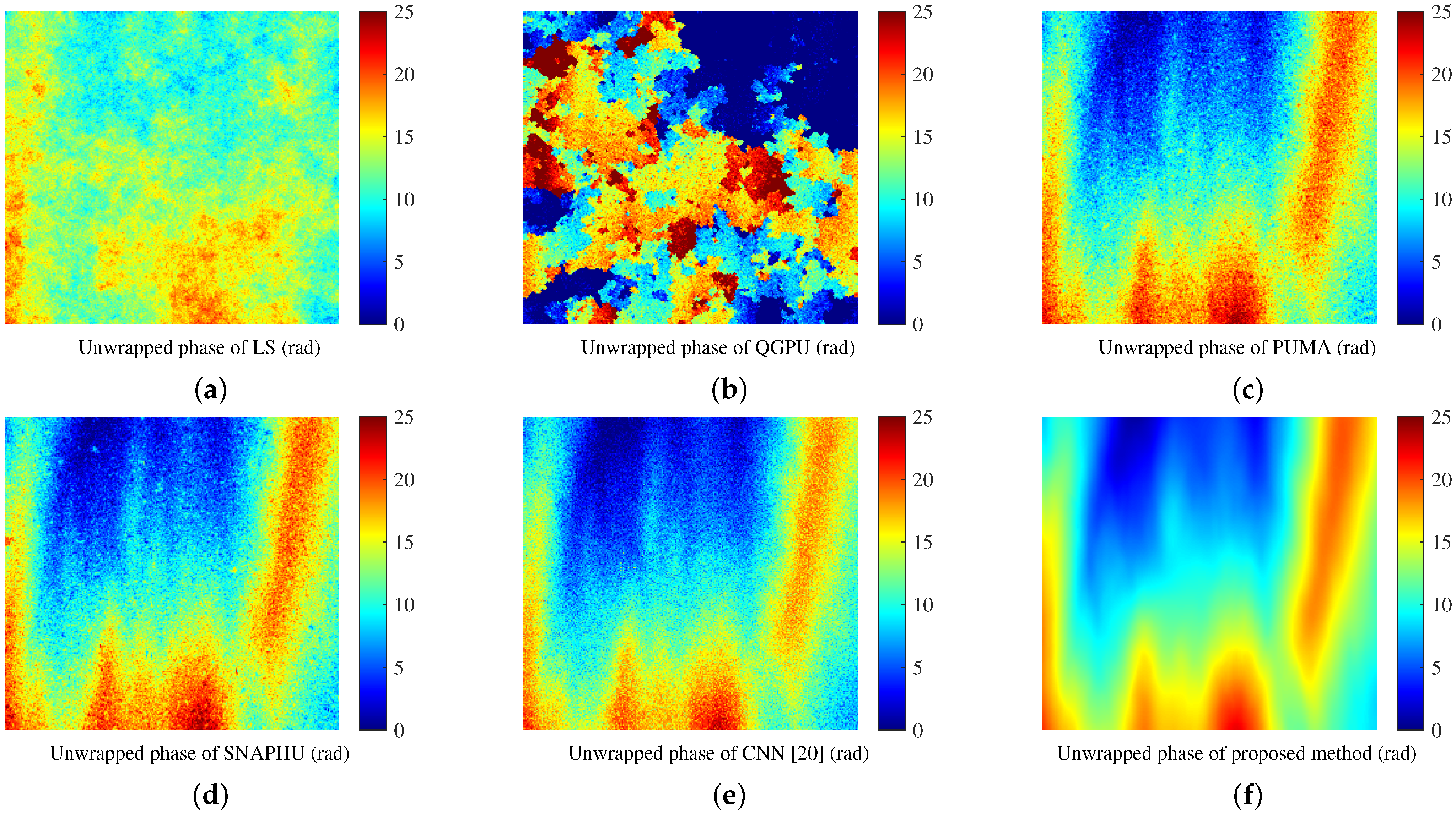
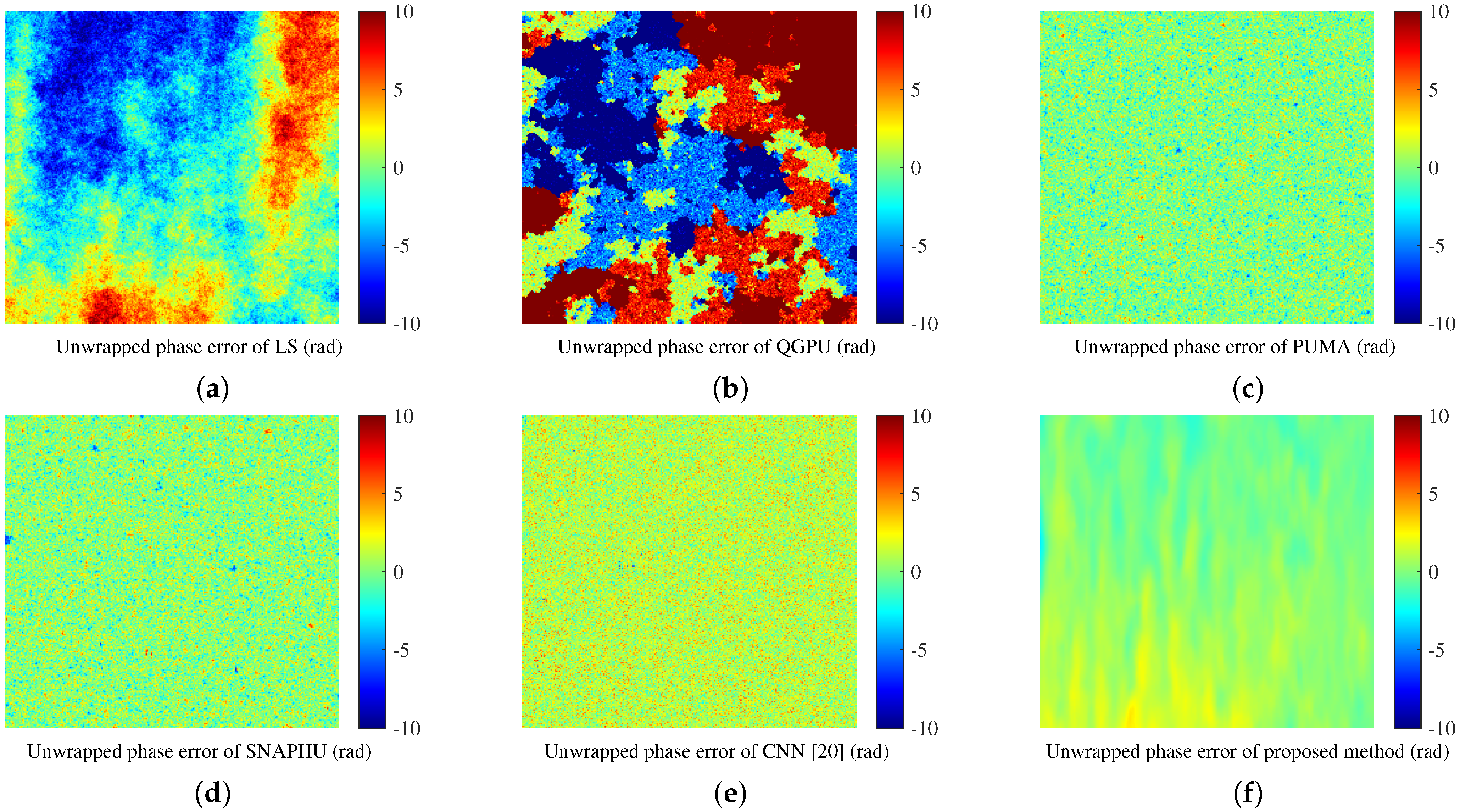
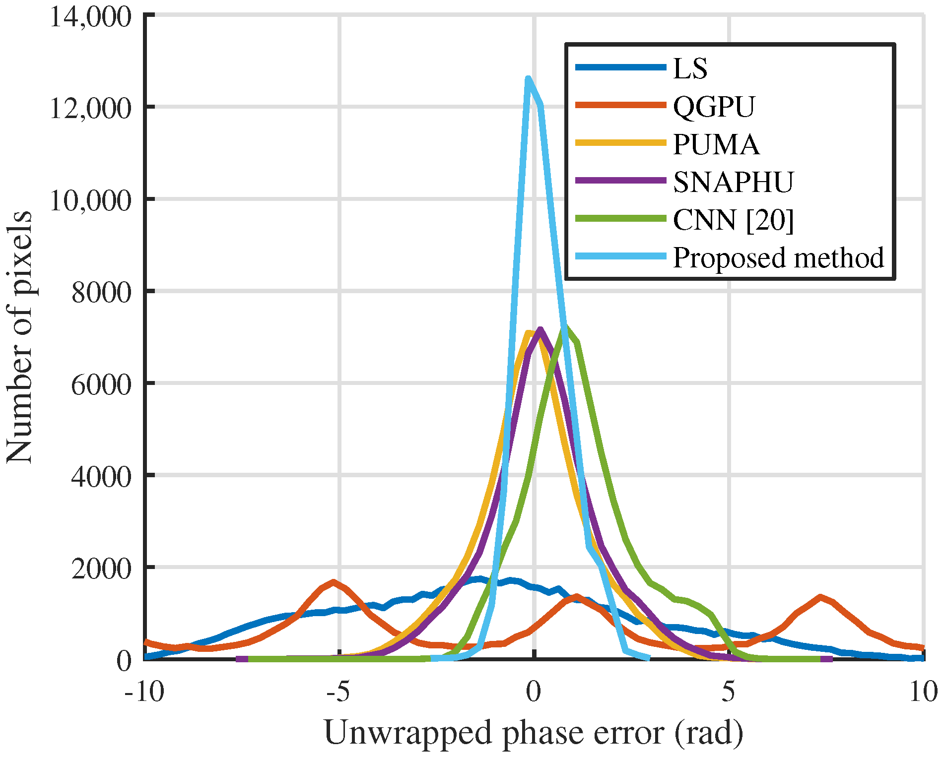
4.3. Performance Evaluation of Phase Unwrapping on Simulated Data

We selected a testing sample with a coherence coefficient of 0.5 (Figure 8b) to analyze the unwrapping accuracy of the proposed method from the perspective of the unwrapped phase error. The proposed method is compared with five widely-used phase unwrapping methods, namely, LS, QGPU, PUMA, and SNAPHU methods, and a deep learning-based method.
The unwrapped phases obtained by these six methods are shown in Figure 13. Figure 14 shows the corresponding errors between the estimated unwrapped phases and ideal unwrapped phase (Figure 8a). We can observe that the unwrapped phase obtained by the propose method is close to the ideal unwrapped phase because most pixels of its error image are close to zero. In order to better quantify the unwrapped phase errors of these six methods, their error histogram curves were fitted and are shown in Figure 15. From Figure 15, compared with the other five unwrapping methods, the error curve of the proposed method is more concentrated near zero and sharper, so the unwrapping accuracy of the proposed method was the highest among these six methods.

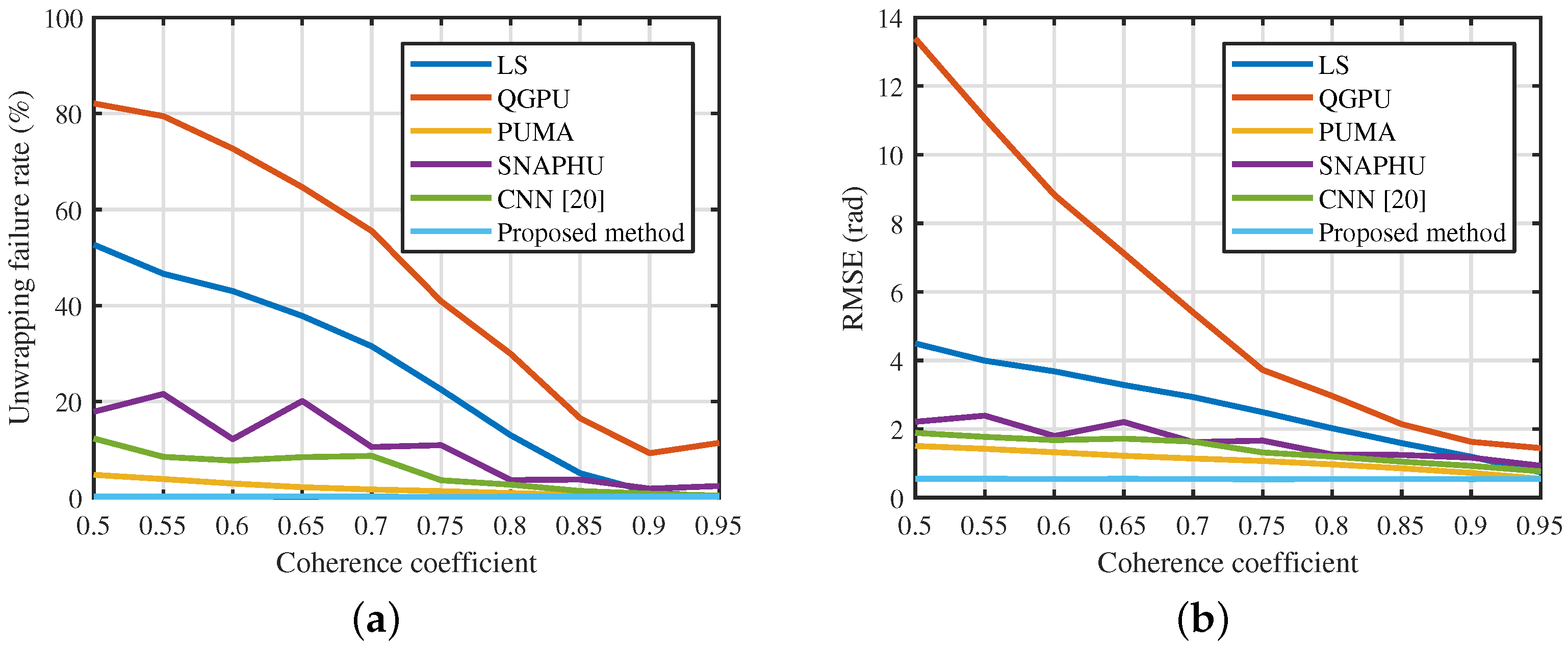
4.4. Robustness Testing of Phase Unwrapping on Simulated Data

As described in Section 3.1, the coherence coefficients of all testing samples ranged from 0.5 to 0.95. For the noise robustness testing, we calculated the mean values of the unwrapping failure rate and RMSE of these six unwrapping methods for the testing samples with the same coherence coefficients, and the results are shown in Figure 16. It can been observed that the proposed method had the smallest unwrapping failure rate and RMSE for each considered coherence coefficient case; that is, among these six unwrapping methods, the proposed method has the highest unwrapping accuracy. Moreover, the unwrapping failure rate and RMSE of the proposed method did not change significantly with the changes in the coherence coefficient, which means the proposed method is robust to noise. To evaluate the comprehensive performance in response to different coherence coefficient situations, the mean values of the unwrapping rate and RMSE for all testing samples were calculated, and are listed in Table 3. We can observe that the unwrapping failure rate and RMSE of the proposed method are the smallest among all six unwrapping methods. Compared with the PUMA method, the unwrapping failure rate and RMSE of the proposed method were 89.3% and 49.5% lower, respectively. Compared with the CNN method [20], the unwrapping failure rate and RMSE of the proposed method were 96.3% and 61.2% lower, respectively. The reason for this performance improvement may be that the classification error is further amplified in the post-processing of the CNN method [20] due to the difference between adjacent categories corresponding to an unwrapped phase of 2 π . Additionally, in the proposed method, the continuous phase gradient estimation can ensure the unwrapped phase error is within a small range. From Figure 14, we can indeed observe that the unwrapped phase error range of the CNN method [20] is significantly larger than that of the proposed method. In addition, the unwrapping failure rate and RMSE of the CNN method [20] increased as the noise level increased, which may be because the classification error increased as the noise level increased. Furthermore, as the level of noise decreased, the performance gaps among the different unwrapping methods gradually decreased. Based on the above analysis, the proposed method has the highest unwrapping accuracy among these six unwrapping method and is robust to noise.

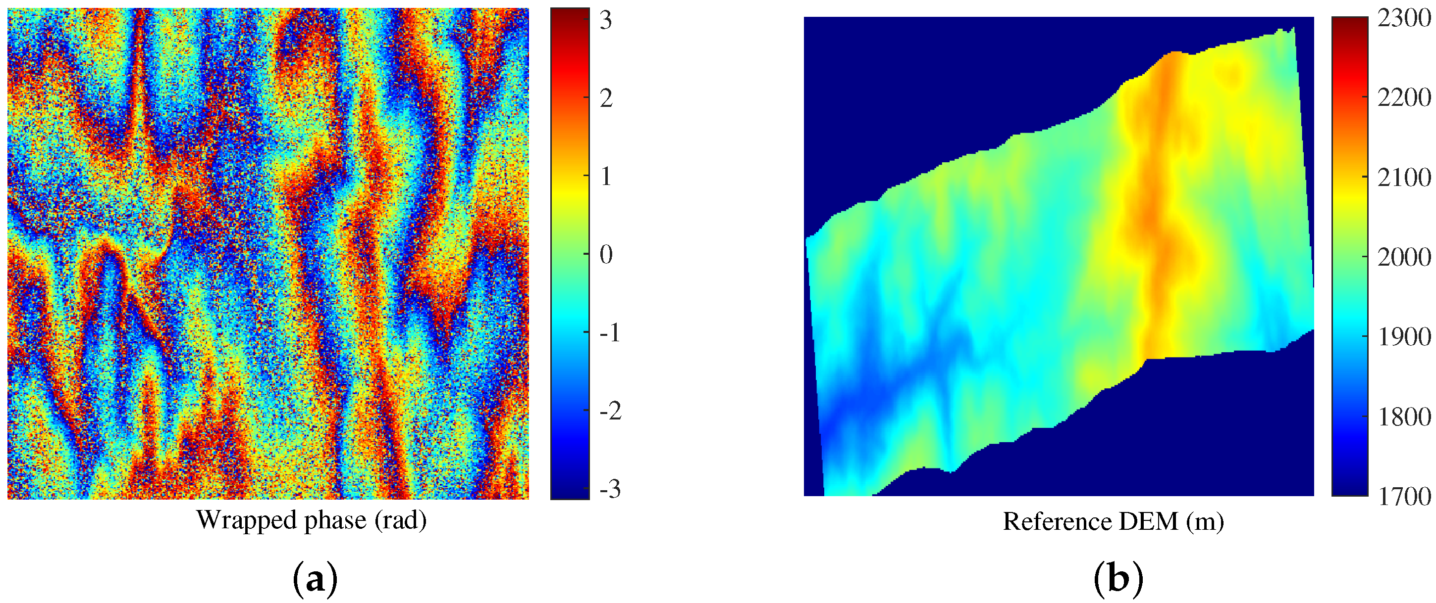
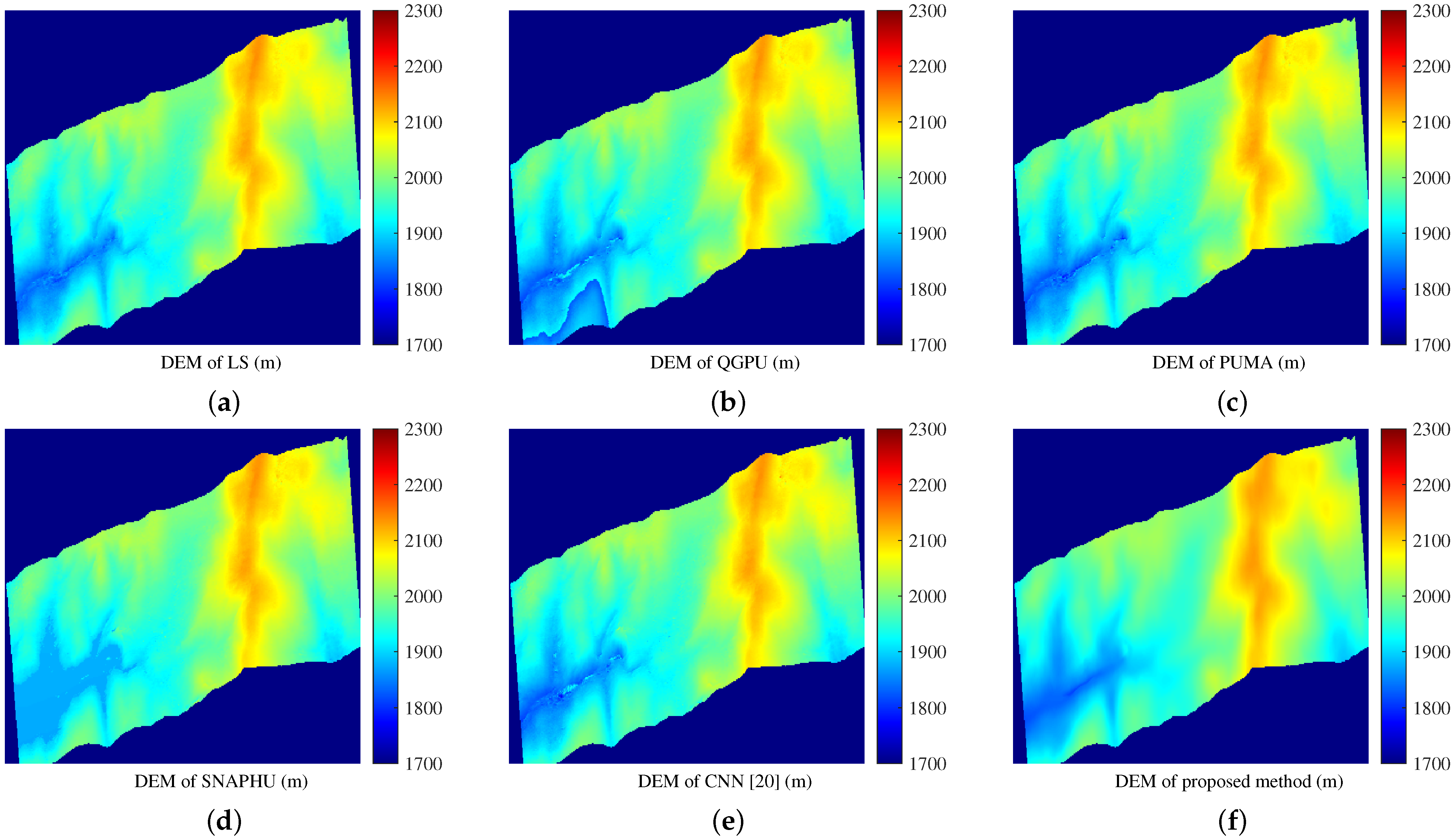
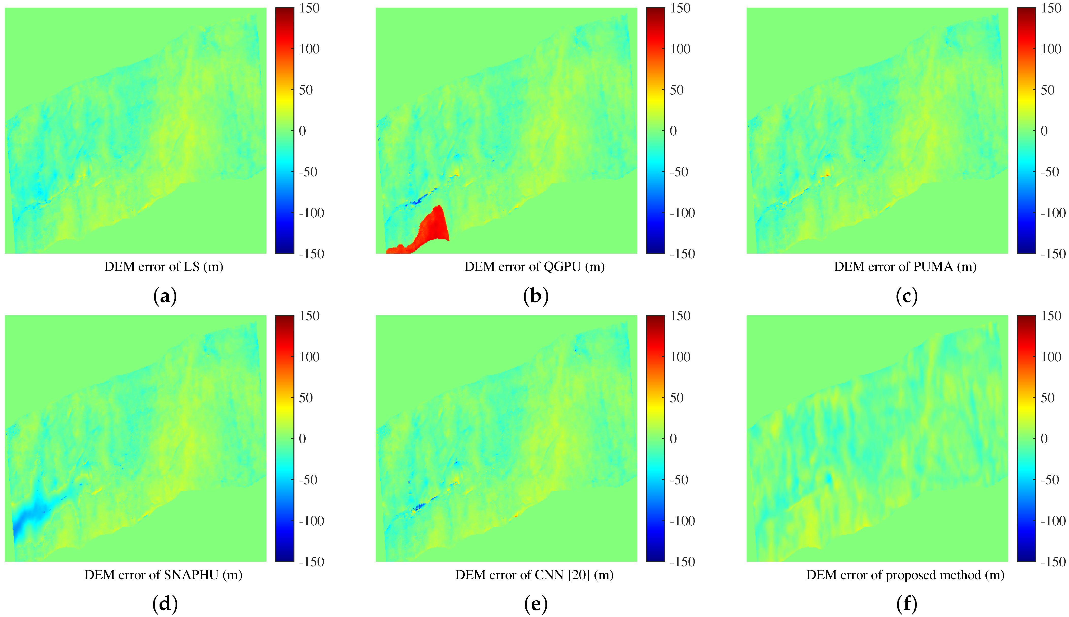
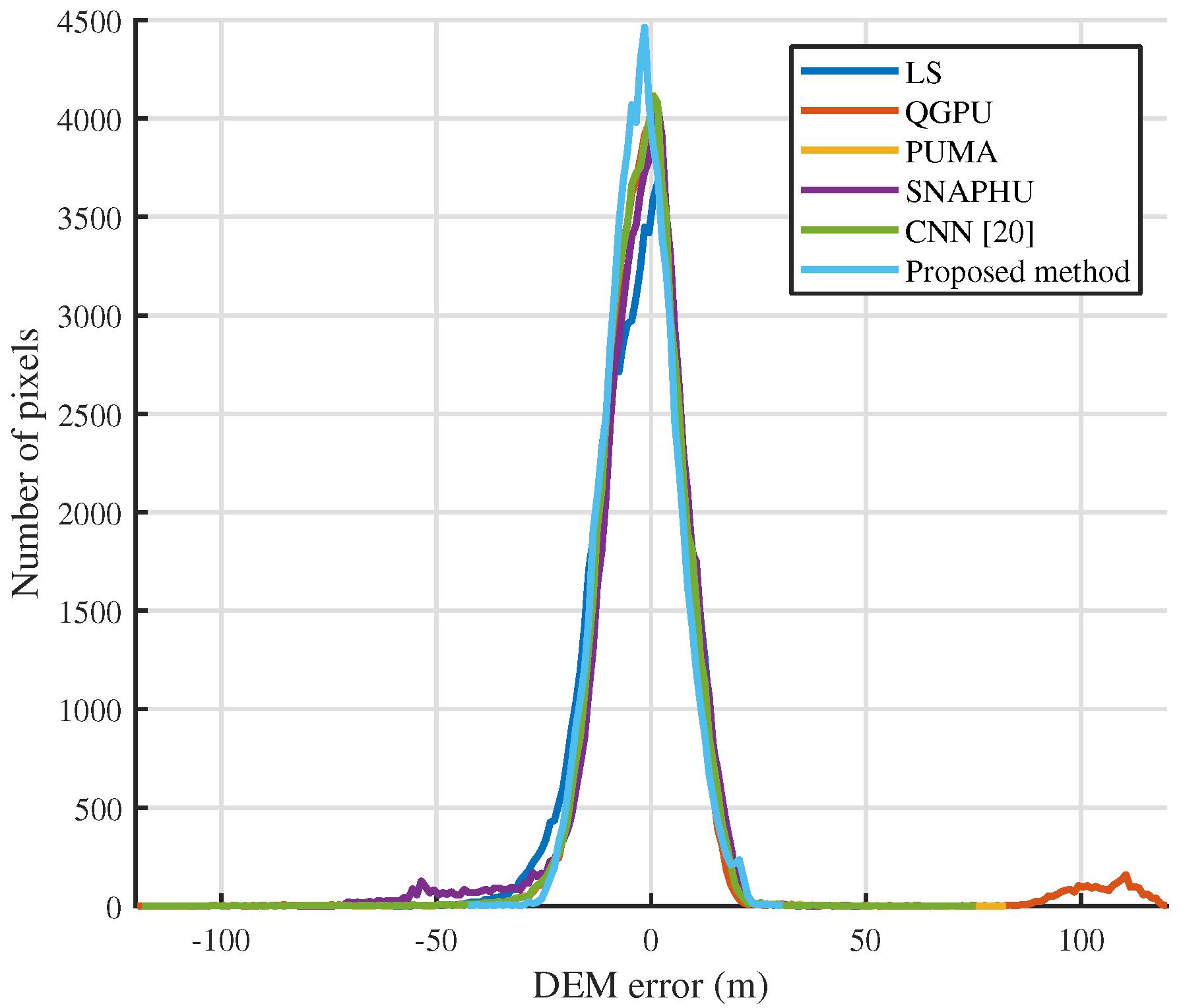
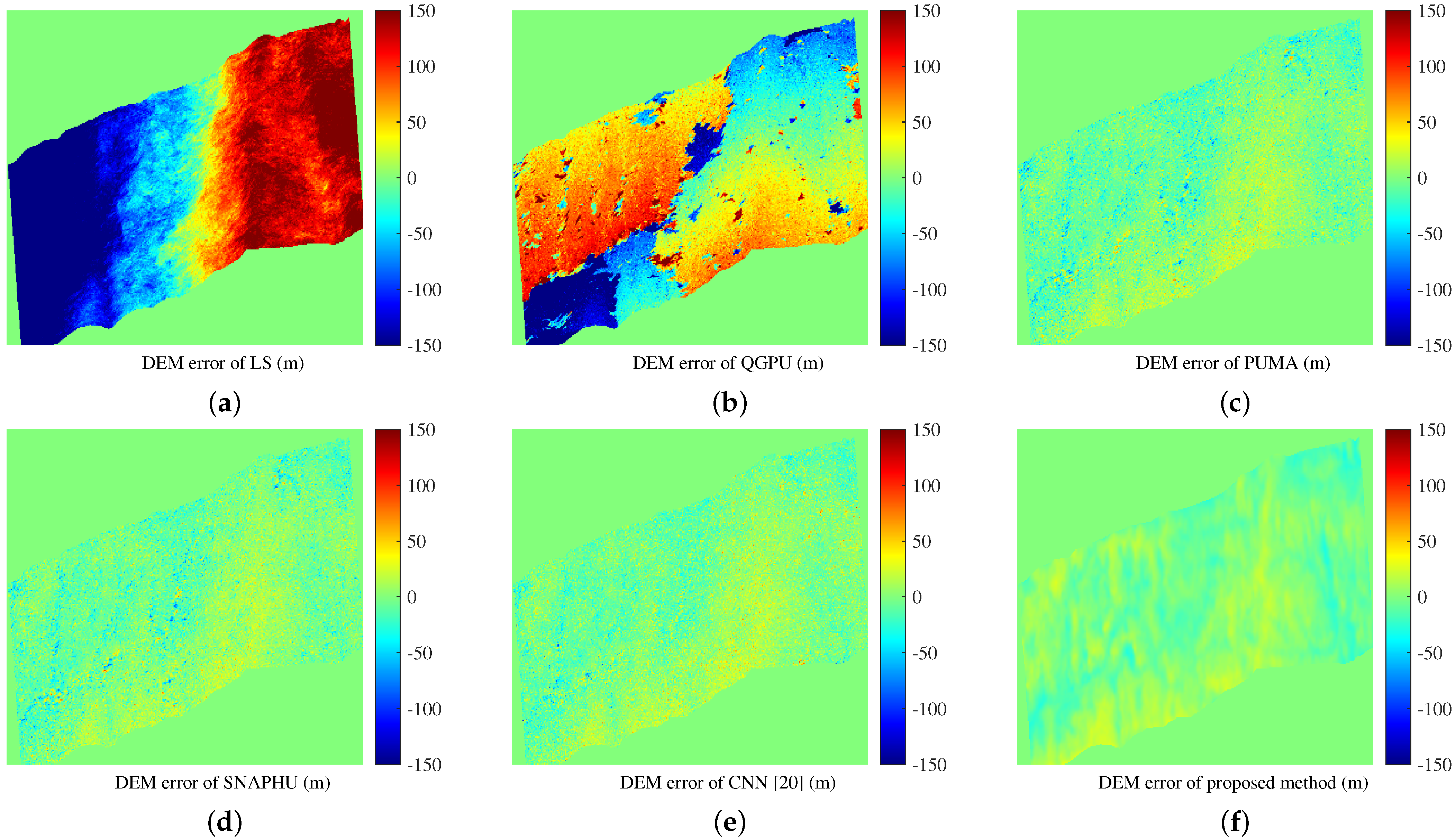
4.5. Performance Evaluation of Phase Unwrapping on Real InSAR Data

A real wrapped phase image was used to evaluate the phase unwrapping performance of the proposed method. The proposed method’s performance is compared with those of other five unwrapping methods. Before unwrapping, the widely-used Goldstein phase filtering algorithm [37] was employed to suppress the noise of the real wrapped phase image. According to the unwrapping results, we performed two operations to obtain the estimated DEM: elevation inversion and terrain correction. This two operations were performed by the standard methods of SNAP software (“Phase to Elevation” and “Range Doppler Terrain Correction”).
The wrapped phase image covering the eastern part of Turkey was computed from a pair of SLC images acquired by the SAR satellite Sentinel-1 Interferometric Wide Swath mode on 2 and 8 July 2019. Figure 17a is the wrapped phase image and Figure 17b is the corresponding reference DEM. The DEM is from SRTM 1Sec HGT and can be downloaded with the official SNAP software; and it was processed using the bilinear interpolation method to match the grid size of the estimated DEM (13.93 m).
In the case of performing phase filtering, the DEM results obtained by the phase unwrapping results of these six unwrapping methods are shown in Figure 18. Figure 19 shows the corresponding errors between the DEM solutions and the reference DEM. We can observe that the DEM obtained by the proposed method is closest to the reference DEM among these six methods because most pixels of its error image are closest to zero. To better quantify the DEM errors of these six unwrapping methods, the histogram error curves were fitted and are shown in Figure 20. From Figure 20, compared with the other five unwrapping methods, the error curve of the proposed method is more concentrated near zero and sharper, so the unwrapping accuracy of the proposed method was the highest among these six methods.
For quantitative evaluation, the RMSE between DEM solutions obtained by these six methods and the reference DEM were calculated and are listed in Table 4. As seen from Table 4, the RMSE of the proposed method is the smallest among these six unwrapping methods. In addition, compared with the PUMA method and CNN method [20], the RMSE of the proposed method is 3.73% or 7.0% lower, respectively. The performance improvement was not as large as with the simulated data, because the noise level was greatly reduced after performing phase filtering. As the level of noise decreases, the performance gaps among different unwrapping methods gradually decreases. Based on the above analysis, the unwrapping accuracy of the proposed method is the highest among these six methods.

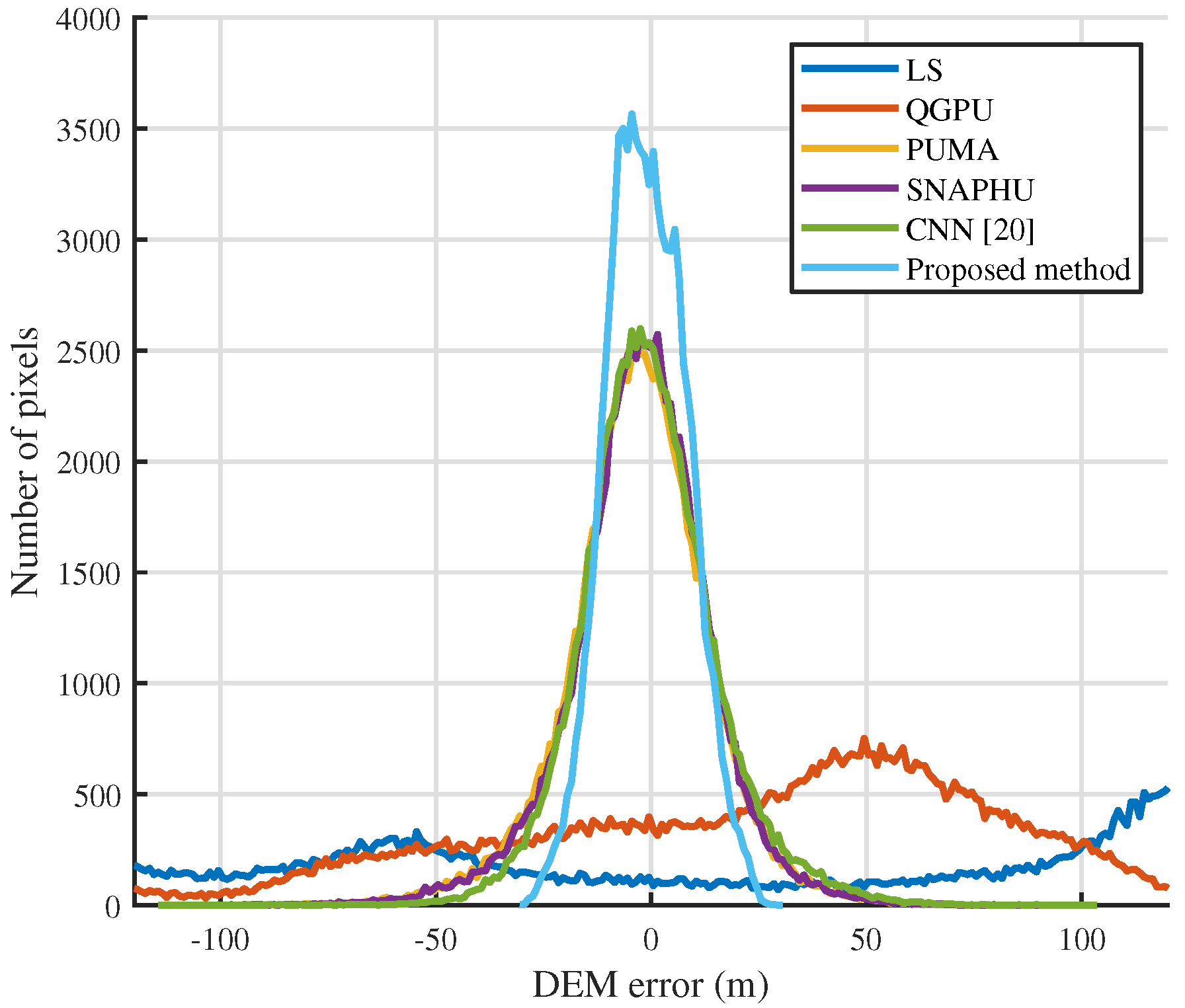
4.6. Robustness Testing of Phase Unwrapping on Real InSAR Data

In real data processing, to improve the accuracy of phase unwrapping, phase filtering is often required before unwrapping, but after filtering, there will still be different levels of noise, and its level depends on the noise suppression performance of the filtering algorithm and the quality of the wrapped phase [38]. To evaluate the robustness of the proposed method, this section shows the DEM estimation results of Figure 17a in the case of no phase filtering.
The DEM results obtained by the phase unwrapping results of these six unwrapping methods without phase filtering are shown in Figure 21. Figure 22 shows the corresponding errors between the DEM solutions and the reference DEM. The histogram error curves were fitted and are shown in Figure 23, and the RMSE between DEM solutions and the reference DEM are listed in Table 5. We can see that the unwrapping accuracy of the proposed method was still the highest among these six methods because the RMSE of the proposed method is smallest. In addition, compared with Section 4.5, the unwrapping results of the LS and QGPU methods are failures, and the performances of the PUMA, SNAPHU, and CNN [20] methods decreased significantly when the noise level became larger because their RMSE increased by 85.04%, 39.60%, and 66.16%, respectively. The performance of the proposed method decreased slightly because its RMSE increased by 7.25%. Based on the above analysis, it can be seen that the proposed method has better anti-noise performance than the other five methods in real data processing.

5. Discussion

To analyze the influence of networks with different block numbers on the unwrapping performance, we complemented three experiments with simulated data, and their numbers of blocks were 10, 8, and 5, respectively. Their RMSE were calculated and are listed in Table 6. As the RMSE of the network with eight blocks were smallest, we selected the network with eight blocks. From Table 3 and Table 6, we can see that different block numbers led to slight fluctuations in RMSE for our method, but the unwrapping performance was still better than those of the other five unwrapping methods.

6. Conclusions

In this paper, a robust InSAR phase unwrapping method combining PGENet and the least squares solver was proposed to improve the accuracy of phase unwrapping. We designed PGENet to estimate the horizontal and vertical gradients first, and then the phase unwrapping result is obtained by using the least squares solver to minimize the difference between the gradient obtained by PGENet and the gradient of the unwrapped phase. The horizontal and vertical gradients estimated by PGENet are used to replace the gradients estimated by PGE-PCA in the traditional LS unwrapping method. PGENet can extract global high-level phase features and recognize the phase gradient between adjacent pixels from lots of wrapped phase images with topography features and different coherence coefficients. Therefore, compared with the phase gradient obtained by PGE-PCA, the more accurate and robust phase gradient can be estimated by PGENet. This is the reason why the proposed method has higher precision and better robustness than the traditional LS unwrapping method. The experimental results on simulated data showed that the proposed method has the highest unwrapping accuracy among six widely-used unwrapping methods and is robust to noise. Furthermore, when processing the real Sentinel-1 InSAR data, the proposed method had the best performance among these six unwrapping methods.
The proposed method successfully combines deep learning and the traditional LS method for InSAR phase unwrapping. The core of this method is the accurate and robust phase gradient estimation based on PGENet, which makes the proposed method have high accuracy and robustness. In future work, to achieve more accurate unwrapping, we will make targeted modifications to PGENet to match more traditional InSAR phase unwrapping methods. In addition, we will use the proposed phase unwrapping method to process more real InSAR data.

Author Contributions

Conceptualization, L.P., X.Z. and J.S.; methodology, L.P. and X.Z.; software, L.P., Z.Z. and S.W.; validation, L.P., Z.Z. and J.S.; formal analysis, L.P., S.W., L.L. and L.Z.; investigation, L.P., Z.Z., L.Z. and L.L.; resources, X.Z. and S.W.; data curation, L.P. and X.Z.; writing—original draft preparation, L.P., X.Z. and J.S.; writing—review and editing, L.P., L.L., L.Z. and S.W.; visualization, L.P., Z.Z., L.L. and L.Z.; supervision, X.Z. and J.S.; project administration, X.Z.; funding acquisition, X.Z. All authors have read and agreed to the published version of the manuscript.

Funding

This research was supported in part by the National Key R&D Program of China under grant 2017YFB0502700, and in part by the National Natural Science Foundation of China under grants 61571099, 61501098, and 61671113.

Institutional Review Board Statement

Not applicable.

Informed Consent Statement

Not applicable.

Data Availability Statement

Not applicable.

Acknowledgments

We thank all editors and reviewers and for their valuable comments and suggestions for improving this manuscript.

Conflicts of Interest

The authors declare no conflict of interest.

References

  1. Moreira, A.; Prats-Iraola, P.; Younis, M.; Krieger, G.; Hajnsek, I.; Papathanassiou, K.P. A tutorial on synthetic aperture radar. IEEE Geosci. Remote Sens. Mag. 2013, 1, 6–43. [Google Scholar] [CrossRef] [Green Version]
  2. Yu, H.; Lan, Y.; Yuan, Z.; Xu, J.; Lee, H. Phase Unwrapping in InSAR: A Review. IEEE Geosci. Remote Sens. Mag. 2019, 7, 40–58. [Google Scholar] [CrossRef]
  3. Zhu, X.; Wang, Y.; Montazeri, S.; Ge, N. A Review of Ten-Year Advances of Multi-Baseline SAR Interferometry Using TerraSAR-X Data. Remote Sens. 2018, 10, 1374. [Google Scholar] [CrossRef] [Green Version]
  4. Bamler, R.; Hartl, P. Synthetic aperture radar interferometry. Inverse Probl. 1998, 14, R1. [Google Scholar] [CrossRef]
  5. Goldstein, R.M.; Zebker, H.A.; Werner, C.L. Satellite radar interferometry: Two-dimensional phase unwrapping. Radio Sci. 1988, 23, 713–720. [Google Scholar] [CrossRef] [Green Version]
  6. Itoh, K. Analysis of the phase unwrapping algorithm. Appl. Opt. 1982, 21, 2470. [Google Scholar] [CrossRef] [PubMed]
  7. Herráez, M.A.; Burton, D.R.; Lalor, M.J.; Gdeisat, M.A. Fast two-dimensional phase-unwrapping algorithm based on sorting by reliability following a noncontinuous path. Appl. Opt. 2002, 41, 7437–7444. [Google Scholar] [CrossRef] [PubMed]
  8. Lin, Q.; Vesecky, J.F.; Zebker, H.A. New approaches in interferometric SAR data processing. IEEE Trans. Geosci. Remote Sens. 1992, 30, 560–567. [Google Scholar] [CrossRef]
  9. Yan, L.; Zhang, H.; Zhang, R.; Xie, X.; Chen, B. A robust phase unwrapping algorithm based on reliability mask and weighted minimum least-squares method. Opt. Lasers Eng. 2019, 112, 39–45. [Google Scholar] [CrossRef]
  10. Bioucas-Dias, J.M.; Valadao, G. Phase unwrapping via graph cuts. IEEE Trans. Image Process. 2007, 16, 698–709. [Google Scholar] [CrossRef]
  11. Zhang, Y.Z.; Wang, W.D.; Li, P. Minimum L 2-norm two dimensional phase unwrapping. J. Earth Sci. Enivron. 2005, 1, 80–83. [Google Scholar]
  12. Pritt, M.D. Phase unwrapping by means of multigrid techniques for interferometric SAR. IEEE Trans. Geosci. Remote Sens. 1996, 34, 728–738. [Google Scholar] [CrossRef]
  13. Ghiglia, D.C.; Romero, L.A. Robust two-dimensional weighted and unweighted phase unwrapping that uses fast transforms and iterative methods. JOSA A 1994, 11, 107–117. [Google Scholar] [CrossRef]
  14. Chen, C.W.; Zebker, H.A. Phase unwrapping for large SAR interferograms: Statistical segmentation and generalized network models. IEEE Trans. Geosci. Remote Sens. 2002, 40, 1709–1719. [Google Scholar] [CrossRef] [Green Version]
  15. Chen, C.W.; Zebker, H.A. Network approaches to two-dimensional phase unwrapping: Intractability and two new algorithms. JOSA A 2000, 17, 401–414. [Google Scholar] [CrossRef] [PubMed]
  16. Liang, J.; Zhang, J.; Shao, J.; Song, B.; Yao, B.; Liang, R. Deep Convolutional Neural Network Phase Unwrapping for Fringe Projection 3D Imaging. Sensors 2020, 20, 3691. [Google Scholar] [CrossRef]
  17. Zhang, T.; Jiang, S.; Zhao, Z.; Dixit, K.; Zhou, X.; Hou, J.; Zhang, Y.; Yan, C. Rapid and robust two-dimensional phase unwrapping via deep learning. Opt. Express 2019, 27, 23173–23185. [Google Scholar] [CrossRef]
  18. Spoorthi, G.; Gorthi, R.K.S.S.; Gorthi, S. PhaseNet 2.0: Phase Unwrapping of Noisy Data Based on Deep Learning Approach. IEEE Trans. Image Process. 2020, 29, 4862–4872. [Google Scholar] [CrossRef]
  19. Li, S.; Xu, H.; Gao, S.; Li, C. A non-fuzzy interferometric phase estimation algorithm based on modified Fully Convolutional Network. Pattern Recognit. Lett. 2019, 128, 60–69. [Google Scholar] [CrossRef]
  20. Sica, F.; Calvanese, F.; Scarpa, G.; Rizzoli, P. A CNN-Based Coherence-Driven Approach for InSAR Phase Unwrapping. IEEE Geosci. Remote Sens. Lett. 2020. early access. [Google Scholar] [CrossRef]
  21. Zhou, L.; Yu, H.; Lan, Y. Deep Convolutional Neural Network-Based Robust Phase Gradient Estimation for Two-Dimensional Phase Unwrapping Using SAR Interferograms. IEEE Trans. Geosci. Remote Sens. 2020, 58, 4653–4665. [Google Scholar] [CrossRef]
  22. Zhou, L.; Yu, H.; Lan, Y.; Xing, m. Artificial Intelligence In Interferometric Synthetic Aperture Radar Phase Unwrapping: A Review. IEEE Geosci. Remote Sens. Mag. 2021, 9, 10–28. [Google Scholar] [CrossRef]
  23. Wang, H.; Hu, J.; Fu, H.; Wang, C.; Wang, Z. A Novel Quality-Guided Two-Dimensional InSAR Phase Unwrapping Method via GAUNet. IEEE J. Sel. Top. Appl. Earth Obs. Remote Sens. 2021, 14, 7840–7856. [Google Scholar] [CrossRef]
  24. Ahmad, A.; Lu, Y. Identifying the phase discontinuities in the wrapped phase maps by a classification framework. Opt. Eng. 2016, 55, 033104. [Google Scholar] [CrossRef]
  25. Costantini, M. A novel phase unwrapping method based on network programming. IEEE Trans. Geosci. Remote Sens. 1998, 36, 813–821. [Google Scholar] [CrossRef]
  26. Pritt, M.D. Weighted least squares phase unwrapping by means of multigrid techniques. In Proceedings of the Synthetic Aperture Radar and Passive Microwave Sensing, Paris, France, 25–28 September 1995; International Society for Optics and Photonics: Paris, France, 1995; Volume 2584, pp. 278–288. [Google Scholar]
  27. Guo, Y.; Chen, X.; Zhang, T. Robust phase unwrapping algorithm based on least squares. Opt. Lasers Eng. 2014, 63, 25–29. [Google Scholar] [CrossRef]
  28. Mao, X.; Shen, C.; Yang, Y.B. Image restoration using very deep convolutional encoder-decoder networks with symmetric skip connections. Adv. Neural Inf. Process. Syst. 2016, 29, 2802–2810. [Google Scholar]
  29. Tao, X.; Gao, H.; Shen, X.; Wang, J.; Jia, J. Scale-recurrent network for deep image deblurring. In Proceedings of the IEEE Conference on Computer Vision and Pattern Recognition, Salt Lake City, UT, USA, 18–23 June 2018; pp. 8174–8182. [Google Scholar]
  30. Ronneberger, O.; Fischer, P.; Brox, T. U-net: Convolutional networks for biomedical image segmentation. In Proceedings of the International Conference on Medical Image Computing and Computer-Assisted Intervention, Munich, Germany, 5–9 October 2015; pp. 234–241. [Google Scholar]
  31. Nah, S.; Hyun Kim, T.; Mu Lee, K. Deep multi-scale convolutional neural network for dynamic scene deblurring. In Proceedings of the IEEE Conference on Computer Vision and Pattern Recognition, Honolulu, HI, USA, 21–26 July 2017; pp. 3883–3891. [Google Scholar]
  32. Zhou, Y.; Shi, J.; Yang, X.; Wang, C.; Kumar, D.; Wei, S.; Zhang, X. Deep multi-scale recurrent network for synthetic aperture radar images despeckling. Remote Sens. 2019, 11, 2462. [Google Scholar] [CrossRef] [Green Version]
  33. Pu, L.; Zhang, X.; Zhou, Z.; Shi, J.; Wei, S.; Zhou, Y. A Phase Filtering Method with Scale Recurrent Networks for InSAR. Remote Sens. 2020, 12, 3453. [Google Scholar] [CrossRef]
  34. Kingma, D.P.; Ba, J. Adam: A method for stochastic optimization. arXiv 2014, arXiv:1412.6980. [Google Scholar]
  35. Yao, Y.; Rosasco, L.; Caponnetto, A. On early stopping in gradient descent learning. Constr. Approx. 2007, 26, 289–315. [Google Scholar] [CrossRef]
  36. Raskutti, G.; Wainwright, M.J.; Yu, B. Early stopping and non-parametric regression: An optimal data-dependent stopping rule. J. Mach. Learn. Res. 2014, 15, 335–366. [Google Scholar]
  37. Goldstein, R.M.; Werner, C.L. Radar interferogram filtering for geophysical applications. Geophys. Res. Lett. 1998, 25, 4035–4038. [Google Scholar] [CrossRef] [Green Version]
  38. Wang, Y.; Huang, H.; Dong, Z.; Wu, M. Modified patch-based locally optimal Wiener method for interferometric SAR phase filtering. ISPRS J. Photogramm. Remote Sens. 2016, 114, 10–23. [Google Scholar] [CrossRef] [Green Version]
Figure 1. Flowchart of the traditional least squares phase unwrapping method.
Remotesensing 13 04564 g001
Figure 2. (a) Wrapped phase images, and (b,c) are the corresponding horizontal gradient images and vertical gradient images, respectively. From top to bottom, the coherence coefficients are 1, 0.95, 0.75, and 0.5, respectively.
Remotesensing 13 04564 g002
Figure 3. Overall architecture of PGENet.
Remotesensing 13 04564 g003
Figure 4. Flowchart of the proposed method.
Remotesensing 13 04564 g004
Figure 5. (a) Reference DEM used for training. (b) Ideal wrapped phase simulated by the reference DEM. (c) Ideal horizontal gradient. (d) Ideal vertical gradient.
Remotesensing 13 04564 g005
Figure 6. Examples of the noisy wrapped phase with different coherence coefficients. (a) 0.5. (b) 0.75. (c) 0.95.
Remotesensing 13 04564 g006
Figure 7. (a) Reference DEM used for testing. (b) Wrapped phase with a coherence coefficient of 0.5. (c) Ideal horizontal phase gradient. (d) Ideal vertical phase gradient.
Remotesensing 13 04564 g007
Figure 8. A testing sample. (a) Ideal unwrapped phase used for performance evaluation. (b) Noisy wrapped phase with a coherence coefficient of 0.5. (c) Ideal horizontal phase gradient. (d) Ideal Vertical phase gradient.
Remotesensing 13 04564 g008
Figure 9. Phase gradient images estimated by two methods. (a) Horizontal phase gradient and (b) vertical phase gradient estimated by PGE-PCA. (c) Horizontal phase gradient and (d) vertical phase gradient estimated by PGENet.
Remotesensing 13 04564 g009
Figure 10. Phase gradient estimation errors. (a) Horizontal gradient error and (b) vertical gradient error of PGE-PCA. (c) Horizontal gradient error and (d) vertical gradient error of PGENet.
Remotesensing 13 04564 g010
Figure 11. Phase gradient error curves. (a) Horizontal phase gradient error. (b) Vertical phase gradient error.
Remotesensing 13 04564 g011
Figure 12. Root mean square errors (RMSE) of two phase gradient estimation methods on simulated data with different coherence coefficients. (a) Horizontal phase gradient estimation. (b) Vertical phase gradient estimation.
Remotesensing 13 04564 g012
Figure 13. Unwrapped phase images of six phase unwrapping methods on simulated data. (a) LS. (b) QGPU. (c) PUMA. (d) SNAPHU. (e) CNN [20]. (f) Proposed method.
Remotesensing 13 04564 g013
Figure 14. Unwrapped phase errors on simulated data. (a) LS. (b) QGPU. (c) PUMA. (d) SNAPHU. (e) CNN [20]. (f) Proposed method.
Remotesensing 13 04564 g014
Figure 15. Fitted unwrapped phase error histogram curves of six phase unwrapping methods on simulated data.
Remotesensing 13 04564 g015
Figure 16. Quantitative indexes of six methods for phase unwrapping results on simulated wrapped phase images with different coherence coefficients. (a) Unwrapping failure rate. (b) Root mean square error (RMSE).
Remotesensing 13 04564 g016
Figure 17. Sentinel-1 InSAR data. (a) Wrapped phase image. (b) Reference DEM.
Remotesensing 13 04564 g017
Figure 18. In the case of performing phase filtering, the DEM results of six phase unwrapping methods on real data. (a) LS. (b) QGPU. (c) PUMA. (d) SNAPHU. (e) CNN [20]. (f) Proposed method.
Remotesensing 13 04564 g018
Figure 19. In the case of performing phase filtering, the DEM errors on real data. (a) DEM errors of the least squares method. (b) DEM errors of QGPU. (c) DEM errors of PUMA. (d) DEM errors of SNAPHU. (e) DEM errors of CNN [20]. (f) DEM errors of the proposed method.
Remotesensing 13 04564 g019
Figure 20. In the case of performing phase filtering, the fitted DEM error histogram curves of six phase unwrapping methods on real InSAR data.
Remotesensing 13 04564 g020
Figure 21. In the case of no phase filtering, the DEM results of six phase unwrapping methods on real data. (a) LS. (b) QGPU. (c) PUMA. (d) SNAPHU. (e) CNN [20]. (f) Proposed method.
Remotesensing 13 04564 g021
Figure 22. In the case of no phase filtering, the DEM errors on real data. (a) DEM errors of the least squares method. (b) DEM errors of QGPU. (c) DEM errors of PUMA. (d) DEM errors of SNAPHU. (e) DEM errors of CNN [20]. (f) DEM errors of the proposed method.
Remotesensing 13 04564 g022
Figure 23. In the case of no phase filtering, the fitted DEM error histogram curves of six phase unwrapping methods on real InSAR data.
Remotesensing 13 04564 g023
Table 1. Detailed parameters of each layer in PGENet.
#Layer NameFilter Size# Feature MapsPaddingStrideImage Size
Encoder Block 1Conv + Relu 5 × 5 6421 M × N × 64
Conv + Relu 5 × 5 6422 M / 2 × N / 2 × 64
Encoder Block 2Conv + Relu 5 × 5 12821 M / 2 × N / 2 × 128
Conv + Relu 5 × 5 12822 M / 4 × N / 4 × 128
Encoder Block 3Conv + Relu 5 × 5 25621 M / 4 × N / 4 × 256
Conv + Relu 5 × 5 25622 M / 8 × N / 8 × 256
Encoder Block 4Conv + Relu 5 × 5 51221 M / 8 × N / 8 × 512
Conv + Relu 5 × 5 51222 M / 16 × N / 16 × 512
Encoder Block 5Conv + Relu 5 × 5 51221 M / 16 × N / 16 × 512
Conv + Relu 5 × 5 51222 M / 32 × N / 32 × 512
Encoder Block 6Conv + Relu 5 × 5 51221 M / 32 × N / 32 × 512
Conv + Relu 5 × 5 51222 M / 64 × N / 64 × 512
Encoder Block 7Conv + Relu 5 × 5 51221 M / 64 × N / 64 × 512
Conv + Relu 5 × 5 51222 M / 128 × N / 128 × 512
Encoder Block 8Conv + Relu 5 × 5 51221 M / 128 × N / 128 × 512
Conv + Relu 5 × 5 51222 M / 256 × N / 256 × 512
Decoder Block 1Conv + Relu 5 × 5 51221 M / 256 × N / 256 × 512
Deconv + Relu 4 × 4 51212 M / 128 × N / 128 × 512
Decoder Block 2Conv + Relu 5 × 5 51221 M / 128 × N / 128 × 512
Deconv + Relu 4 × 4 51212 M / 64 × N / 64 × 512
Decoder Block 3Conv + Relu 5 × 5 51221 M / 64 × N / 64 × 512
Deconv + Relu 4 × 4 51212 M / 32 × N / 32 × 512
Decoder Block 4Conv + Relu 5 × 5 51221 M / 32 × N / 32 × 512
Deconv + Relu 4 × 4 51212 M / 16 × N / 16 × 512
Decoder Block 5Conv + Relu 5 × 5 25621 M / 16 × N / 16 × 256
Deconv + Relu 4 × 4 25612 M / 8 × N / 8 × 256
Decoder Block 6Conv + Relu 5 × 5 12821 M / 8 × N / 8 × 128
Deconv + Relu 4 × 4 12812 M / 4 × N / 4 × 128
Decoder Block 7Conv + Relu 5 × 5 6421 M / 4 × N / 4 × 64
Deconv + Relu 4 × 4 6412 M / 2 × N / 2 × 64
Decoder Block 8Conv + Relu 5 × 5 3221 M / 2 × N / 2 × 64
Deconv + Relu 4 × 4 3212 M / 2 × N / 2 × 32
Conv + Relu 5 × 5 121 M × N × 1
Table 2. A comparison of two phase gradient estimation methods using root mean square error (RMSE) on simulated data with different coherence coefficients.
MethodsHorizontal Phase GradientVertical Phase Gradient
RMSE (Rad)RMSE (Rad)
PGE-PCA2.162.14
PGENet0.090.03
Table 3. Quantitative indexes of six phase unwrapping methods on simulated data.
MethodsUnwrapping Failure Rate (%)RMSE (Rad)
LS25.352.64
QGPU46.245.77
PUMA1.871.07
SNAPHU10.491.65
CNN [20]5.451.39
Proposed method0.200.54
Table 4. In the case of performing phase filtering, the comparison of six phase unwrapping methods using root mean square error (RMSE) on real InSAR data.
MethodsRMSE (m)
LS8.00
QGPU15.16
PUMA7.02
SNAPHU9.09
CNN [20]7.27
Proposed method6.76
Table 5. In the case of no phase filtering, the comparison of six phase unwrapping methods using root mean square error (RMSE) on real InSAR data.
MethodsRMSE (m)
LS110.89
QGPU64.08
PUMA12.99
SNAPHU12.69
CNN [20]12.08
Proposed method7.25
Table 6. Root mean square errors (RMSE) of the proposed method in networks with different numbers of blocks.
Number of BlockRMSE (rad)
100.6039
80.5425
50.6150
Publisher’s Note: MDPI stays neutral with regard to jurisdictional claims in published maps and institutional affiliations.

