Article

Estimating Ground Elevation and Vegetation Characteristics in Coastal Salt Marshes Using UAV-Based LiDAR and Digital Aerial Photogrammetry

1
Department of Civil and Coastal Engineering, University of Florida, Gainesville, FL 32603, USA
2
School of Forest Resources and Conservation, University of Florida, Gainesville, FL 32611, USA
3
Department of Mechanical and Aerospace Engineering, University of Florida, Gainesville, FL 32611, USA
*
Author to whom correspondence should be addressed.
Remote Sens. 2021, 13(22), 4506; https://doi.org/10.3390/rs13224506
Submission received: 27 September 2021 / Revised: 4 November 2021 / Accepted: 7 November 2021 / Published: 9 November 2021
(This article belongs to the Special Issue UAV for High-Resolution Salt Marsh Monitoring)

Abstract

:
This study evaluates the skills of two types of drone-based point clouds, derived from LiDAR and photogrammetric techniques, in estimating ground elevation, vegetation height, and vegetation density on a highly vegetated salt marsh. The proposed formulation is calibrated and tested using data measured on a Spartina alterniflora-dominated salt marsh in Little Sapelo Island, USA. The method produces high-resolution (ground sampling distance = 0.40 m) maps of ground elevation and vegetation characteristics and captures the large gradients in the proximity of tidal creeks. Our results show that LiDAR-based techniques provide more accurate reconstructions of marsh vegetation (height: MAEVH = 12.6 cm and RMSEVH = 17.5 cm; density: MAEVD = 6.9 stems m−2 and RMSEVD = 9.4 stems m−2) and morphology (MAEM = 4.2 cm; RMSEM = 5.9 cm) than Digital Aerial Photogrammetry (DAP) (MAEVH = 31.1 cm; RMSEVH = 38.1 cm; MAEVD = 12.7 stems m−2; RMSEVD = 16.6 stems m−2; MAEM = 11.3 cm; RMSEM = 17.2 cm). The accuracy of the classification procedure for vegetation calculation negligibly improves when RGB images are used as input parameters together with the LiDAR-UAV point cloud (MAEVH = 6.9 cm; RMSEVH = 9.4 cm; MAEVD = 10.0 stems m−2; RMSEVD = 14.0 stems m−2). However, it improves when used together with the DAP-UAV point cloud (MAEVH = 21.7 cm; RMSEVH = 25.8 cm; MAEVD = 15.2 stems m−2; RMSEVD = 18.7 stems m−2). Thus, we discourage using DAP-UAV-derived point clouds for high-resolution vegetation mapping of coastal areas, if not coupled with other data sources.

1. Introduction

Salt marshes are essential environments that provide ecological and anthropologic functions, such as storm attenuation [1,2], carbon sequestration, and water quality enhancement [3,4,5,6]. In the last decades, coastal marsh systems suffered a progressive conversion to open water areas and mudflats due to sea-level rise (SLR), climate change, and anthropogenic impact [4,7,8,9,10]. Additionally, it is estimated that, by 2100, up to 50% of global wetland will be lost, depending on the evolution of SLR, human activity, and the availability of accommodation space facilitating wetland migration [4,10,11,12]. The reduction in salt marsh extent limits the ecosystem functions, endangering human communities living in coastal areas. In the US alone, coastal communities represent ~30% of the total population [13].
Effective monitoring methods are required to address the loss of these valuable habitats. Monitoring marsh morphology and vegetation can provide insight into the response of these ecosystems to environmental and anthropogenic stressors. Ground elevation dictates the tidal prism [14], and the marsh hydroperiod [15], thus regulating vegetation growth over the marsh. Vegetation mitigates the impact of meteorological and hydrodynamic forcing [16], controls organic and inorganic deposition rates in the marsh system [17], and deflects water fluxes over less vegetated regions, thus modulating marsh platform flooding [18,19]. Accurate knowledge of these processes is fundamental to maximize the effectiveness of marshland preservation and management. This is generally achieved using numerical models [20,21,22]. Because an accurate description of both ground elevation and vegetation will improve the models, this will also have beneficial implications on marsh preservation.
Traditional approaches to determine marsh ground elevation and vegetation characteristics are based on in situ surveys [23,24,25]. Although these approaches allow collecting precise data on the marshland, they are intrusive, are limited by domain accessibility, and require significant effort to collect and process a dataset [26]. Alternative non-intrusive remote sensing technologies are used to study coastal environments. These methods mostly use imagery, multispectral, and point clouds datasets, coupled with statistical analysis, machine learning techniques, and custom methods to evaluate ground elevation, as well as vegetation characteristics in various environments. In the past, several studies had been based on satellite images to estimate morphology and vegetation properties of salt marshes [6,26,27]. However, due to the limited spatial resolution of the datasets, and the high dependency on atmospheric conditions of these technologies [26,28,29,30,31], they had been progressively replaced by or coupled with manned or Unmanned Aerial Vehicles (UAVs) [19,31,32,33]. In particular, due to their rapid technological advancement, UAVs are becoming standard technology for high-resolution coastal [34,35,36] and agricultural [37,38] survey and mapping.
Light Detection and Ranging (LiDAR) is a remote sensing technology based on lasers. It is usually associated with aircraft or UAVs to monitor land surfaces. Aircraft are generally preferred to UAVs to survey larger areas rapidly, at the expense of the spatial resolution of the collected datasets [39]. Airborne LiDARs have been widely used to survey coastal wetlands [31,40], and salt meadows [32], as well as for forestry applications [41,42,43,44,45]. Airborne LiDAR had also been coupled with other remote sensing datasets, which lack tridimensionality and adequate spatial resolution to supply this information. Satellite data were associated with LiDAR to map wetland flooding [46], vernal pools [47], and coastal wetlands landscape and vegetation characteristics [48,49,50,51,52]. Optical images were also coupled with LiDAR point clouds for vegetation classification purposes [53,54,55].
In the last decade, airborne LiDARs have valuably increased their spatial resolution, reaching point densities of 50–120 points m−2 [42,56]. However, their resolution is still not comparable with UAV-based LiDAR, which can reach point densities >500 points m−2 [57]. A possible solution to increase airborne LiDAR’s resolution is to scan the same area multiple times, which inevitably increases the monetary and analysis cost of the survey. Another solution is to reduce the flight altitude of the aircraft, which reduces the laser beam footprint and consequently increases the time and the cost of the survey. Especially in vegetated coastal areas, where a large density of points is necessary to resolve large gradients in bed elevation and vegetation characteristics and to minimize the screening effect of the dense vegetation on the creek levees [19,23], UAVs are generally preferred to aircraft. This depends on the elevated density of the collected point clouds, but also on the capability UAVs have to follow the path of meandering rivers and tidal creeks, and on the low cost and flexibility of the surveys [23,58].
An alternative technique used to survey point clouds is based on Terrestrial Laser Scanners (TLS). TLSs gave good results in estimating vegetation in different habitats [59,60]. However, they suffer the following limitations. To survey large areas, many TLSs are required. This is because the point cloud should be surveyed at the same time, or in a short time frame. The use of a large number of TLSs implies: (i) a higher cost of the survey; (ii) a higher cost, in terms of time and people needed to dispose and remove the TLSs in the field; (iii) a higher impact of the survey on the surveyed area, due to the movement of surveyor and tools in the field. In addition, previous studies underlined that TLSs suffer strong limitations in areas where dense ground vegetation predominates [59,60], such as salt marshes. Dense vegetation layers reduce the penetration of laser beams, especially in the areas scanned with a high incident angle. Indeed, laser penetration is high only in the limited area close to the scanner, where laser beams are perpendicular to the ground. The effect of the incident angle is low using UAVs, which allow to survey the area from a nadir perspective.
A low-cost alternative to LiDAR to acquire point clouds is Structure from Motion (SfM) photogrammetry [61,62] (or Digital Aerial Photogrammetry, DAP). This technique reconstructs 3D point clouds by overlapping multiple 2D images and using the distances calculated between the image key points [63]. DAP applications are various and include agricultural mapping [64], 3D modeling of complex structures [65], and the identification of vegetation structures [66,67]. DAP has shorter and less intricate flight paths than LiDAR. Moreover, it has lower errors on vertical elements and the adjacent area [68]. In addition, DAP is scale-invariant [69], and the camera resolution is the only limit of the output images and point clouds [63]. However, compared with LiDAR, DAP shows: (i) lower performances to estimate forest variables [70,71] due to low accuracy, even if in some cases, the two data sources demonstrated to be interchangeable or complementary [72,73]; (ii) higher errors due to glares and shadows [74]; (iii) possible surface discontinuities in the collected datasets [75]; (iv) higher time-consuming data processes [68,76,77,78], even if, due to the substantial research conducted on remote sensing image mosaicking, and the presence of numerous commercial software [78], this limitation has been partially reduced; (v) the lower penetration of dense vegetation layers in comparison with LiDAR [75,79].
Many studies compared the performances SfM and LiDAR point clouds have when they are used to describe topographic and vegetation features on urban environments [68], forests, [71,72,80,81,82], and post-mining applications [73,75]. For example, recent studies analyzed the possibility to extract accurate Digital Elevation Models (DEMs) and Digital Terrain Models (DTMs) from UAV-DAP point clouds under open forest canopies, by using different approaches, based on classification, and ground-points filtering methods [83,84,85,86,87]. Accuracies of the DEMs and DTMs derived from DAP-UAV are generally evaluated against ground filtered Aerial LiDAR datasets, by using statistical predictors, such as root-mean-square error (RMSE). For example, Graham et al. [85] found RMSE lower than 1.50 m for the DTM defined in a conifer forest. Jensen et al. [87] found that SfM overestimates lidar-modeled ground height with a mean difference of 0.19 m. In addition, Guerra-Hernández et al. [86], found an RMSE of 0.19 m estimating tree height in a Pinus pinea plantation using an SfM technique. An analysis between RMSE, ground slope, and canopy cover distributions, underlines their strong relationship [83,85]. In addition, a few studies estimated ground elevation and vegetation characteristics in a salt marsh using either LiDAR- or DAP-UAV point clouds [23,49,79,88].
However, a study comparing the results obtained using LiDAR- and DAP-UAV point clouds, in a cordgrass-populated salt marsh, does not exist. For this reason, our work consists of the first comparison between LiDAR and Photogrammetry in a salt marsh environment. With our work, we aim to fill this gap, by comparing the spatial distribution of ground elevation and vegetation characteristics (height and density) obtained from a LiDAR- and a DAP-UAV dataset we collected on a Spartina alterniflora vegetated salt marsh system in Little Sapelo Island, Georgia, USA, (Figure 1). The LiDAR and DAP point clouds are georeferenced using a Total station and 27 Ground Control Points (GCPs), respectively. The ground elevation and vegetation characteristics (height and density) distributions are obtained by applying the machine learning algorithm (Genetic Algorithm, GA) proposed in Pinton et al. (2020) [23] to both point clouds. The algorithm is previously trained, validated, and tested for both point clouds, through a rigorous leave-one-out cross-validation (LOOCV) procedure, by using ground elevation data, which were collected using an RTK-GPS, vegetation density, and vegetation height data, which were manually collected in the marsh. LiDAR- and DAP-UAV distributions are then compared, and the RMSE of the differences obtained for each variable is calculated.

2. Data and Methods

2.1. Study Site

Our study site is located at the south-eastern boundary of Little Sapelo Island, Georgia, USA (Figure 1b), and is located in the Georgia Coastal Ecosystem Long Term Ecological Research (GCELTER) (Figure 1a). The site is a 0.26 km2 portion of a vegetated marsh system, which is flanked by the Duplin River at the eastern side and crossed by eleven creeks. Various cordgrass species populate the environment, but the predominant one is Spartina alterniflora [89,90]. It occupies the creek banks, the low marsh, and the marsh edge with heights up to 2 m [91], and the high marsh with heights up to 0.60 m. The local tide gauge (NOAA, n. #8675761) indicates that the tide has a semi-diurnal cycle and can reach a water level of ~1.6 m MSL during spring tides, submerging the marsh with a water layer of ~1 m.

2.2. Field Measurements

Field measurements were performed on the 22 November 2019, at low tide, to limit the presence of water on the marsh platform and the creeks, and its interference on the fieldwork.

2.2.1. Ground Control Points

In the study area, we placed twenty-seven Ground Control Points (GCPs). The GCPs were uniformly distributed to cover the entire salt marsh system. The upper part of the GCPs was a 0.30 m × 0.30 m target, made of a wooden panel. The panel was painted with red and black matte paint (Figure 2a), to make it visible in the imagery dataset we collected, and to avoid possible glares and reflections due to the sun. The wooden plate was set on a 2-m-tall T-post. To avoid being covered by water and tall Spartina alterniflora, each GCP was placed in the ground for half of the pole’s length. Once we set the GCPs, we collected the geographic position of their midpoint using a Trimble R6 GNSS GPS-RTK, which has ±2 cm of vertical accuracy, and ±1 cm horizontal accuracy.

2.2.2. Ground Elevation and Vegetation Survey

We laid out and surveyed sixty-eight 0.40 m × 0.40 m plots (Figure 2b) over the study area. In each plot, we surveyed the geographic position of the midpoint with the GPS-RTK system. For each location, the midpoint of the plot (Figure 2b) was identified as the intersection of the two diagonals, obtained by intersecting a couple of nylon strings. Once the midpoint of the plot was identified, a 5 cm × 5 cm × 0.2 cm plastic plate was placed on its position, gently pressed in the soil for its thickness (0.2 cm). The RTK-GPS measurement was obtained by placing the lower part of the pole on this plate, to avoid its sink. The average PDOP and HDOP we observed for the survey are equal to 2.54 and 1.45, respectively. The respective standard deviations are equal to 0.254 and 0.093. The vegetation height and density were manually taken. They correspond to the average height and the total number of stems in each plot, respectively. The spatial distribution of the plots was chosen to uniformly cover both the domain area and the range of the vegetation height and density in the marsh system. We also added nine plots to the dataset. Because these plots were placed in unvegetated areas located close to the creek heads, we assigned null vegetation height and density values to them. Those plots were not originally included in the RTK-GPS survey and have been added a posteriori to increase the size of the dataset.

2.3. Remote Sensing Survey

2.3.1. LiDAR-UAV Point Cloud

A UAV-borne LiDAR was employed to survey the study domain on the 22nd of November 2019. The survey was performed at low tide, to avoid water on the marsh platform and the creeks. To perform the survey, we employed a custom-built LiDAR system, based on a Velodyne VLP-16 Puck LiDAR, and mounted on a DJI Matrice 600 airframe (Figure 2c). The Velodyne sensor we used has a 903 nm wavelength. The scanner has 16 beams, acquires ~600,000 points s−1, and is georeferenced by a GNSS receiver and a Novatel STIM-300 Intertial Measurement Unit. We post-processed the GNSS data using a local base station and OPUS (https://www.ngs.noaa.gov/OPUS/ (accessed on 7 November 2021)).
To acquire our data, the flight altitude and line spacing were set to 40 m and 50 m, respectively. The average density of the collected point cloud is ~500 points m−2. The dataset was collected in the UTM WGS84 17N geodetic system, considering the WGS84 ellipsoid for the elevation data. To test the LiDAR-UAV point cloud accuracy, we identified the geographic coordinates (X, Y, and Z) of the GCPs centroids, and we compared them with the values surveyed in the field using the RTK-GPS (see Section 2.2.1). The mean absolute horizontal and vertical error corresponds to 0.019 m and 0.050 m, respectively. The horizontal and vertical RMSE correspond to 0.023 m and 0.062 m, respectively.
Finally, although the short vegetation did not allow the differentiation between different returns of the laser impulse, Pinton et al. (2020) [23] showed that a single return is sufficient to describe both the ground elevation, vegetation height, and density in a coastal marsh. The results obtained by D. Wang et al. (2017) [92] in densely vegetated grasslands and Nie et al. (2018) [40] in coastal wetlands, using a single return laser impulse, confirm this assumption.

2.3.2. Imagery Dataset

On the 26th of October 2019, we flew a DJI Phantom 4 Pro UAV on the study domain, to collect the imagery (RGB) dataset. Images were collected from a nadir perspective, at the highest resolution (5472 × 3648 pixels), with a 3:2 aspect ratio, by using the 20-megapixel camera mounted on the UAV gimbal. Images were collected with a lateral and longitudinal overlap of 80%. We chose a flight altitude of 105 m. Consequently, images have a footprint of ~175 m × 115 m on the ground, and a pixel spacing of ~3 cm.
We used the collected RGB images as inputs for the Pix4DMapper software (Release 4.4.12), which gave us a point cloud as output. We used the default software settings to determine the point cloud, which had an average density of ~500 points m−2. This density is very close to the density of the LiDAR-UAV point cloud (see Section 2.3), and corresponds, on average, to a GSD of ~4 cm. Pix4DMapper used the coordinates of the GCPs to georectify the point cloud in their geographic and vertical elevation systems. The program uses a semi-automated georeferencing approach, which requires manual identification of the GCPs. We identified each GCP midpoint in different groups of seven images. To circumvent distortion errors, we avoided images containing the GCPs on their sides. The calculated point cloud lays on the same reference system as the LiDAR-UAV point cloud.
To test the DAP-UAV point cloud accuracy, we identified the geographic coordinates (X, Y, and Z) of the GCPs centroids, and we compared them with the values surveyed in the field using the RTK-GPS (see Section 2.2.1). The mean absolute horizontal and vertical error corresponds to 0.032 m and 0.089 m, respectively. The horizontal and vertical RMSE correspond to 0.050 m and 0.104 m, respectively.

2.3.3. Point Clouds Post-Processing

We used the same procedure to filter both the LiDAR- and DAP-UAV point clouds. We first applied a filter to remove the points lower than 1.20 m below MSL and higher than 2.50 m above MSL. These points described the Duplin River surface and the freshwater forest located at the north-western edge of the domain, respectively. We then applied a second filter to remove the points outside the study domain. We performed the filters using the CloudCompare software (Release 2.11).
We then divided the LiDAR- and DAP-UAV point clouds into subsets by using a 2737 × 1379 grid, of 0.40 m × 0.40 m cells. Gridlines are oriented northward and eastward, and each cell is identified by the indices “n” (north) and “e” (east). We defined the subset of points of the chosen cloud (LiDAR- and DAP-UAV) in the cell (n,e), and the 3 × 3 cell stencil centered in (n,e) as PCn,e, and STn,e, respectively. Here, we use the term "stencil" as it is used in computational fluid dynamics, i.e., in the sense of a geometric arrangement of nodes (our grid cell centers) that relate to the node of interest [93,94]. As in Pinton et al. (2020) [23], we select a 1.20 m × 1.20 m stencil, which was shown to minimize the estimation error in both flat and non-flat areas.

2.4. Ground Elevation and Vegetation Properties Estimation

2.4.1. Point Cloud Transformation Algorithm

In this study, to perform our analysis, we used the algorithm proposed by Pinton et al. (2020) [23]. In the following, we recall only some relevant background from our earlier paper ([23]). The algorithm structure is fully reported in Appendix A.
The algorithm improves the estimate of ground elevation and vegetation characteristics for sloping ground. Standard approaches that employ point clouds use the minimum elevation of the points over a specific area (or “cell”) to estimate the ground elevation. This estimate is assigned to the center of the cell. The area has to be small enough so that the minimum elevation represents the elevation at its center, and large enough to increase the chance that at least a point describes the ground. For a non-flat ground, these approaches can produce a large error, since a point located in a less elevated region is taken as the minimum and assigned to the center. To avoid this problem, the algorithm uses the point cloud to estimate a real ground surface approximation and uses this approximation to transform a sloping-ground case into a flat-ground case. The minimum elevation ( z   S T n , e m i n , see Appendix A) was taken on this transformed point cloud, thus reducing the estimation error.
The algorithm was applied to both the LiDAR- and DAP-UAV point clouds. To determine the bed elevation, we performed a linear regression (Section 3.1) between z   S T n , e m i n and the surveyed ground elevations. The vegetation characteristics (height and density) were obtained from the machine learning technique described in the next section, which uses as inputs (i.e., predictors) the statistical quantities we estimated from the transformed point clouds (see Section 2.5.2) and the imagery dataset (see Section 2.5.3).

2.4.2. Genetic Algorithm

We used a regression model based on a Genetic Algorithm to calculate vegetation characteristics (height and density) at each cell (n,e). The GA simulates a biological evolution process, where an initial population, constituted of random individuals, evolves over consecutive stages until it reaches the optimal composition, which resembles the composition of the target population [95]. At each generational step, the individuals composing the next step are chosen by a fitness function, which is calibrated on the target population. In our study: (i) the individuals were the predictors calculated from the LiDAR-UAV, DAP-UAV, and RGB datasets (see Table 1), (ii) the population changes based on the fitness function (iii), which was the linear regression function the algorithm used to fit the input data, and it was calibrated using as evaluation metric the Root Mean Square Error (RMSE). Finally, (iv) the target population was the ground elevation and vegetation characteristic data collected at each plot.
Genetic algorithms have many advantages over traditional optimization algorithms [96,97]. In particular, the reasons why we preferred a GA to other techniques are: (i) the possibility to be used even with small datasets; (ii) the possibility to obtain as output a formulation, which is based on the assigned model predictors and could be directly adopted for classification procedures. This could be directly adopted for classification procedures and allows an immediate interpretation of the contribution of the model predictors to describe the considered target population.
Some limitations of GA are: (i) the high computational cost, which is compensated by its possibility to be parallelized; (ii) the correct choice of appropriate model predictors, because any inappropriate choice will limit the algorithm converge or it increases the chance to obtain meaningless results [96]. This limitation was resolved by using the most informative predictors obtainable from our datasets (Section 2.5.1).

2.5. Leave-One-Out Cross-Validation Procedure

To train and validate the transformation method and the GA, we used to estimate ground elevation, vegetation height, vegetation density, and we performed a LOOCV. Thus, we split the dataset in two: the training/validation and the test subsets, respectively. The training/validation subset contains ~75% of the “TV” data points collected on the field. With this subset, we trained the algorithms using TV-1 data points, we validate the algorithms on the remaining data points, and we calculate the training and prediction errors. We repeated this procedure for all the TV permutations of the training/validation subset. We then used the average prediction and training errors to verify the performances of the models at the training and validation steps. Once the algorithms are validated, we tested them on an independent dataset, constituted of the remaining ~25% of the fieldwork dataset. Once the algorithms were tested, we finally used the whole dataset to determine the regression formulas and calculate the ground elevation and vegetation characteristics.
We used the 68 plots where the ground elevation was surveyed using the GPS-RTK (see Section 2.2.2) to train, validate, and test the algorithm used to calculate the bed elevation. The data collected in 50 and 18 plots, corresponding to ~75% and ~25% of the dataset, compose the validation and test subsets, respectively. To train, validate, and test the algorithm used to calculate the vegetation characteristics, we used the 77-plot dataset constituted of the 68 plots where the ground elevation was surveyed and the nine plots at the creek heads, where vegetation height and density are set equal to zero (see Section 2.2.2). The 68 plots were divided as we did for the ground elevation (50 + 18 plots). We then randomly split the 9 additional plots, and we assigned 7 (~75%) points to the training/validation dataset and the remaining 2 (~25%) to the test dataset. By doing that, the resulting training/validation dataset contains 57 points and the test dataset 20 points.

2.5.1. Model Predictors

The following sections list and describe the twenty predictors (i.e., input data) of the GA, we identified from the remote sensing datasets. In particular, we calculated eight of them from the transformed point clouds (see Appendix A, Equation (A6)), and 12 from the imagery (RGB) dataset. The list of the model predictors, for each dataset, is reported in Table 1. Notice that the predictors we used in this paper do not differ from the ones commonly used in the literature for land classification purposes, using LiDAR and imagery datasets [89,90,92,98]. The main difference is in the higher resolution of these data, and consequently, the higher amount of information they can provide the GA to describe the local topography and vegetation characteristics.
The following equation describes the standardization procedure we used for on each predictor P :
P ^ = P P ¯ S D P   ,
where P ^ , P ¯ , and S D P are the standardized value, the mean, and the standard deviation of the model predictor, respectively.

2.5.2. Model Predictors from the Point Clouds

This section summarizes the model predictors we computed in STn,e, by using the relative elevations (see Appendix A, Equation (A6)) of the transformed LiDAR- and DAP-UAV point clouds. For readability, hereinafter, “n,e” replaces STn,e when it is used as a subscript. Moreover, we used the index “s” to indicate the generic point of the transformed point cloud contained in STn,e.
The maximum elevation z n , e m a x reads:
z n , e m a x = max   s S T n , e z s r e l   .
Considering that z n , e m i n is null for the transformed point clouds, Δ z n , e corresponds to z n , e m a x .
The mean elevation value z n , e m e a n is calculated as:
z n , e m e a n = s S T n , e z s r e l M n , e   ,
where M n , e is the number of points of the point cloud in STn,e.
The standard deviation σ n , e is expressed as:
σ n , e = s S T n , e z s r e l z n , e m e a n 2 M n , e 1   .
The skewness S n , e is calculated as:
S n , e = 1 M n , e s S T n , e z s r e l z n , e m e a n 3 1 M n , e s S T n , e z s r e l z n , e m e a n 2 3 / 2   .
The kurtosis K n , e reads:
K n , e = 1 M n , e s S T n , e z s r e l z n , e m e a n 4 1 M n , e s S T n , e z s r e l z n , e m e a n 2 2   .
We also calculate the mode z n , e m o d e and the median z n , e m e d i a n for the point cloud in STn,e. To calculate the mode, we divide the transformed point cloud belonging to STn,e into six equivalent vertical layers. We then identified the layer containing the maximum number of points, and we indicated its average elevation as the mode. Finally, we identified the median as the elevation separating the higher and the lower halves of the point cloud in each STn,e. The value is unique for odd M n , e . For even M n , e instead, we averaged the two middle elevation values.
The first column of Table 1 contains all these predictors.

2.5.3. Model Predictors from the Imagery (RGB) Dataset

To calculate the RGB predictors, we first divided the orthomosaic we created from the collected imagery database (see Section 2.3.2) by using the same regular 2737 × 1379 grid of 0.40 m × 0.40 m cells we used to divide the point clouds. For each (n,e) cell, we identified the R (red), G (green), B (blue), and GRAY (grayscale) intensity value of the pixels contained in the 3 × 3 stencil (STn,e) centered in (n,e). The predictors are the minimum (min), maximum (max), and mean of these intensity values.
The second column of Table 1 contains these predictors.

2.6. Error Analysis

The error of the estimated ground elevation and vegetation characteristics was estimated using the Mean Absolute Error (MAE) and the RMSE. When MAE and RMSE are close to zero, the model has good estimation skills. Values were calculated as:
MAE = i = 1 N y o y p r N   ,
RMSE = i = 1 N y o y p r 2 N   ,
where yo are the observed data and ypr are the predicted quantities in the ith sampling location. N is the dimension of the dataset.

3. Results

3.1. Ground Elevation Estimate

The method proposed by Pinton et al. (2020) [23] was used to calculate ground elevation from transformed LiDAR- and DAP-UAV point clouds. To evaluate the performance of the model, we used the LOOCV procedure reported in Section 2.5. To estimate bed elevation ( B L n , e , c l o u d m e t h o d ), we performed a linear regression between surveyed and computed ground elevations values. The regression reads:
  B L n , e , c l o u d m e t h o d = a + b   ·   z n , e , c l o u d m i n , m e t h o d   ,
where z n , e , c l o u d m i n , m e t h o d are the bed elevations corresponding to: (method 1) the elevation of the lowest point of the non-transformed point cloud belonging to STn,e; (method 2) the elevation of the lowest point of the transformed point clouds belonging to STn,e. The transformation is performed by using the regression plane in Equation (A2) (see Appendix A). The methods are applied to both LiDAR- and DAP-UAV point clouds. In Equation (9), “a” and “b” are the linear regression coefficients. We set b = 1 [23], which means that we are looking for a shift equal to “a” that corrects the bias over the entire marsh, independently from the ground elevation.
Table 2 shows the values of MAE and RMSE for all the steps of the cross-validation procedure of the two regression methods applied to both LiDAR- and DAP-UAV point clouds. The errors show similar trends for the two point clouds. Errors are higher for the creek samples than for the marsh samples. Errors obtained for the whole dataset are similar to the ones obtained for the marsh samples. For both the marsh and the entire dataset, DAP error is mostly ~50–150% larger than LiDAR errors, but in two cases, it reaches ~200%. For the creek dataset, DAP errors are ~5–110% larger than LiDAR ones. Values of MAE and RMSE obtained for the test and training/validation phase with the LiDAR database are similar (difference in the errors smaller than 30%), thus confirming the accuracy of the survey method. On the contrary, significant differences in the errors for the test and training/validation phases are seen for the DAP-UAV database (difference ±75%).
The regression methods were then applied to the entire dataset for both the LiDAR- and DAP-UAV datasets, obtaining the coefficients in Table 3. The coefficient “a” is the intercept of the linear regression formula and the bias of the regression model. When the ground elevation is calculated using the original (i.e., non-transformed) point cloud in STn,e, the coefficient “a” is equal to 1.3 and 5.5 cm for the LiDAR- and DAP-UAV datasets, respectively (Table 3, first row). When the ground elevation is calculated using the transformed point cloud, “a” is equal to -1.8 and -0.7 cm for the LiDAR- and DAP-UAV datasets, respectively (Table 3, second row).
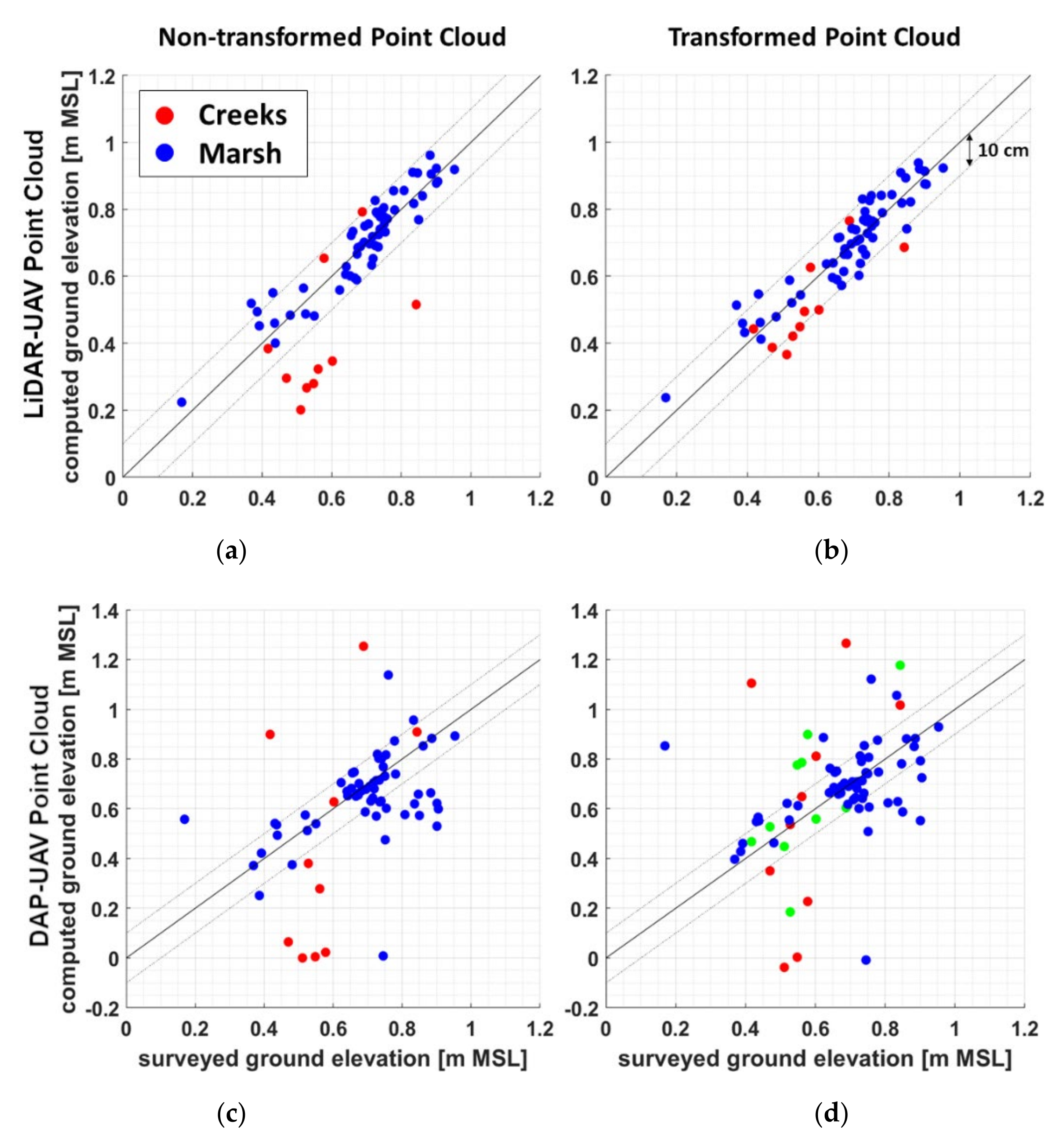
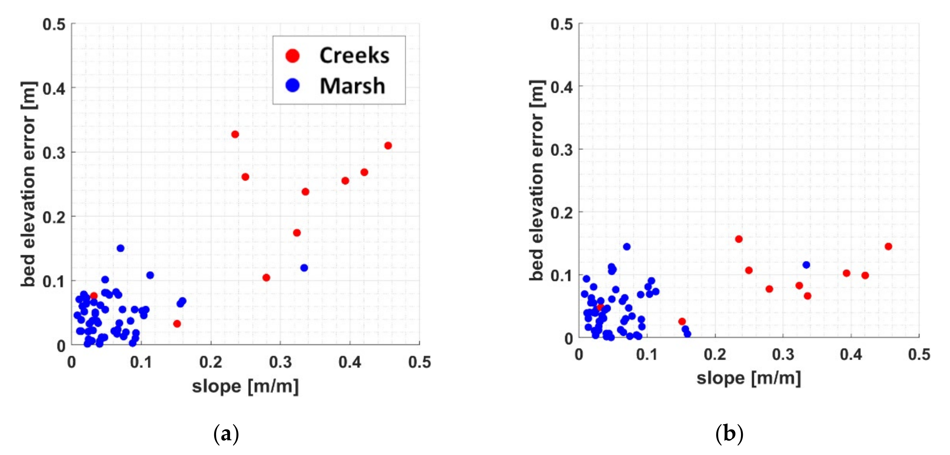
Figure 3a,b compare the measured ground elevation with the values calculated by the non-transformed and transformed LiDAR-UAV point clouds, respectively. The values related to plots surveyed in the marsh platform and on the creeks are reported in blue and red, respectively. The values of RMSE and MAE obtained for the two methods and distinguished between the creek, marsh, and creek plus marsh plots, are reported in the “Test” columns of Table 2, for the dataset indicated as LiD (LiDAR). From Figure 3a,b, a significant underestimation of ground elevation is not observed for the LiDAR-UAV point cloud due to the higher penetration into the vegetation layer and the precise georeferencing of the point cloud due to the employed collection procedure (Section 2.3). For the non-transformed point cloud, a larger underestimation is obtained on the creek banks (red points in Figure 3a). The transformation method (Figure 3b) produces a small overestimation of the ground elevation (second row in Table 3). Figure 3b shows that the transformation strongly reduces the errors for the surveys next to the creeks (red dots). Figure 4a confirms, for the LiDAR-UAV dataset, the dependency of the ground estimation error on the local ground slope, whose value is higher for the plots surveyed close to the creeks (red dots) than in the marsh platform (blue dots). Figure 4b confirms that our model reduces the effect of ground slope on the ground elevation estimation error for the LiDAR-UAV dataset, and makes them comparable to the ones observed in the marsh platform.
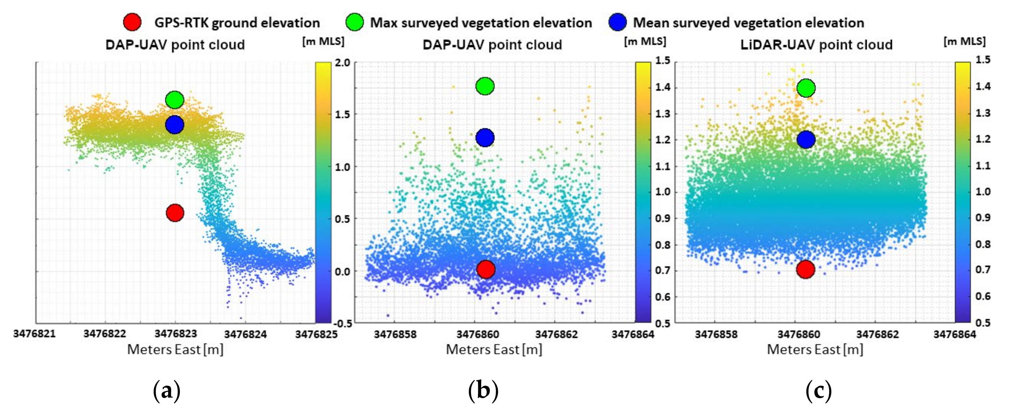
Figure 3c compares the measured ground elevation with the values calculated from the non-transformed DAP-UAV point cloud. The values of RMSE and MAE obtained for this method and distinguished between the creek, marsh, and creek plus marsh plots, are reported in the “Test” columns of Table 2, in the first row related to the DAP-UAV dataset. The comparison in Figure 3c shows a marked misestimation of the ground elevation (>±10 cm) in many of the surveyed points, and a higher tendency of ground level to be underestimated. The strongest underestimation is obtained for the points located on the creek banks (red points in Figure 3c). This happens because, for a 1.20 m × 1.20 m stencil located on the creek bank, the minimum elevation of the point cloud can be given by points on the creek bed, which is ~0.4-0.5 m below the levee elevation. When the ground slope is used to transform the DAP-UAV point cloud (Figure 3d), the error for the creek points is slightly reduced or even amplified in some cases. This is also observed in the values of RMSE and MAE obtained for this method (fourth row) in the creek, marsh, and creek plus marsh plots, as indicated in the “Test” columns of Table 2. These variations happen because a non-accurate estimate of the ground elevation in the nine cells’ center of the stencil (see Appendix A, green dots in Figure 3b) implies a non-accurate estimate of the ground slope through Equation (A2) (see Appendix A). We observed that, for the points located on the creek banks, the upper part of the vegetation is correctly described by the point cloud. We obtained this point by applying the method proposed by Pinton et al. (2020) [23] on the local maxima instead of the minima. We then calculated the ground elevation for each plot by subtracting the maximum vegetation height we manually collected in the field from the elevation of the local maxima we obtained from the LiDAR-UAV point cloud. The results, reported in Figure 3d using green dots, underline a slight improvement, compared to the standard method (red dots). Indeed, in the figure, the MAE observed for the point on the creek banks decreased from 33.4 to 16.4 cm. Finally, for points surveyed on the marsh platform (blue points in Figure 3d), the error is generally low. This happens because, in this area, the low vegetation density and height facilitate the identification of points closer to the marsh ground. Moreover, the low slope of the marsh platform reduces the impact of the point cloud transformation on the error, which indeed shows a negligible difference compared to the one obtained when the transformation is not performed.
For a comparative purpose, the distribution of the ground elevation was estimated by using both the transformed LiDAR- and DAP-UAV point clouds.

3.2. Vegetation Height and Density Estimates

In this section, we present the GA results we obtained by using the predictors derived from the transformed LiDAR- and DAP-UAV point clouds and the RGB images, to estimate the vegetation height and density. The evaluation metrics, corresponding to RMSE and MAE, are reported in Table 4 for all the steps of the validation procedure (train, validation, and test) and all the considered datasets (LiDAR-UAV, DAP-UAV, LiDAR-UAV plus RGB, DAP-UAV plus RGB). Table 4 contains the results for both vegetation height and density. The results of the LiDAR-UAV-based datasets are taken from Pinton et al. (2020) and are reported for a comparative purpose.
For the vegetation height, the metrics have similar values in all the phases of the validation procedure. Here, we comment only on the values obtained in the test phase of the LOOCV. The first row of Table 4 shows that the GA has good predictive skills when it uses only LiDAR predictors to estimate vegetation height. This is due to the higher penetration of LiDAR than DAP in vegetation, which allows the collection of a denser and more accurate point cloud in the vegetation layer. In particular, we obtained an MAE and RMSE equal to 12.6 m and 17.5 cm, respectively. The third row of Table 4 shows that the addition of RGB to LiDAR-UAV-derived predictors slightly reduces the errors obtained using only the LiDAR-UAV predictors. Thus, MAE and RMSE decrease to 10.0 cm and 14.0 cm, respectively. Extremely poor predictive capabilities are obtained by using the DAP-UAV point cloud (Table 4, second row) to estimate vegetation height. The resulting MAE and RMSE are equal to 31.1 cm and 38.1 cm, respectively. Finally, the fourth row of Table 4 shows that the combination of RGB and DAP-UAV-derived predictors gives MAE and RMSE equal to 21.7 cm and 25.8 cm, respectively, which are ~10 cm lower than those obtained for the DAP-UAV dataset.
We estimate vegetation density using the additional predictor B n , e (as in Pinton et al., 2020 [23]), which is a proxy for the biomass, and is defined as:
B n , e = Δ z n , e · V n , e D s u r v e y e d   ,
where V n , e D s u r v e y e d is the vegetation density measured on the marsh.
There is a good agreement between the evaluation metrics of the test and validation stages for the vegetation density. As for the vegetation height, we comment only on the results obtained for the test phase of the LOOCV. The first and third rows of Table 4 show that the MAE and RMSE obtained from the LiDAR-UAV and the LiDAR-UAV plus RGB datasets predictors, are the same. Their value is equal to 6.9 stems m−2 and 9.4 stems m−2, respectively. Because the surveyed range for vegetation density is ~200 stems m−2, the error is ~5%. We consider this a good result. In addition, the error for the DAP-UAV and DAP-UAV plus RGB datasets show similar results (Table 4, second and fourth rows), but higher than the ones observed for the LiDAR-UAV datasets. In particular, the RMSE is equal to 16.6 and 18.7 stems m−2, and the MAE is equal to 12.7 and 15.2 stems m−2.
Finally, once the model was validated and tested, we used the entire database (77 samples) and the predictors obtained from LiDAR- and DAP-UAV point clouds, to determine the formulations describing the vegetation height and the vegetation density over the studied salt marsh. For the LiDAR-UAV dataset, the relationships are the following ones, which are also reported in Pinton et al. (2020) [23]:
V n , e , L i D A R H ^ = 0.92   σ n , e , L i D A R ^   ,
B n , e , L i D A R ^ = 0.39   σ n , e , L i D A R ^ + z n , e , L i D A R m e d i a n ^   .
For the DAP-UAV dataset we obtained the following relationship:
B n , e , L i D A R ^ = 0.39   σ n , e , L i D A R ^ + z n , e , L i D A R m e d i a n ^   .
The relationships underline the importance of the σ n , e ^ (i.e., the standard deviation) in describing the vegetation properties on a densely vegetated salt marsh. Moreover, they underline the importance the RGB parameters assume when coupled with a DAP-UAV point cloud to estimate the vegetation properties.

3.3. Ground Elevation and Vegetation Maps

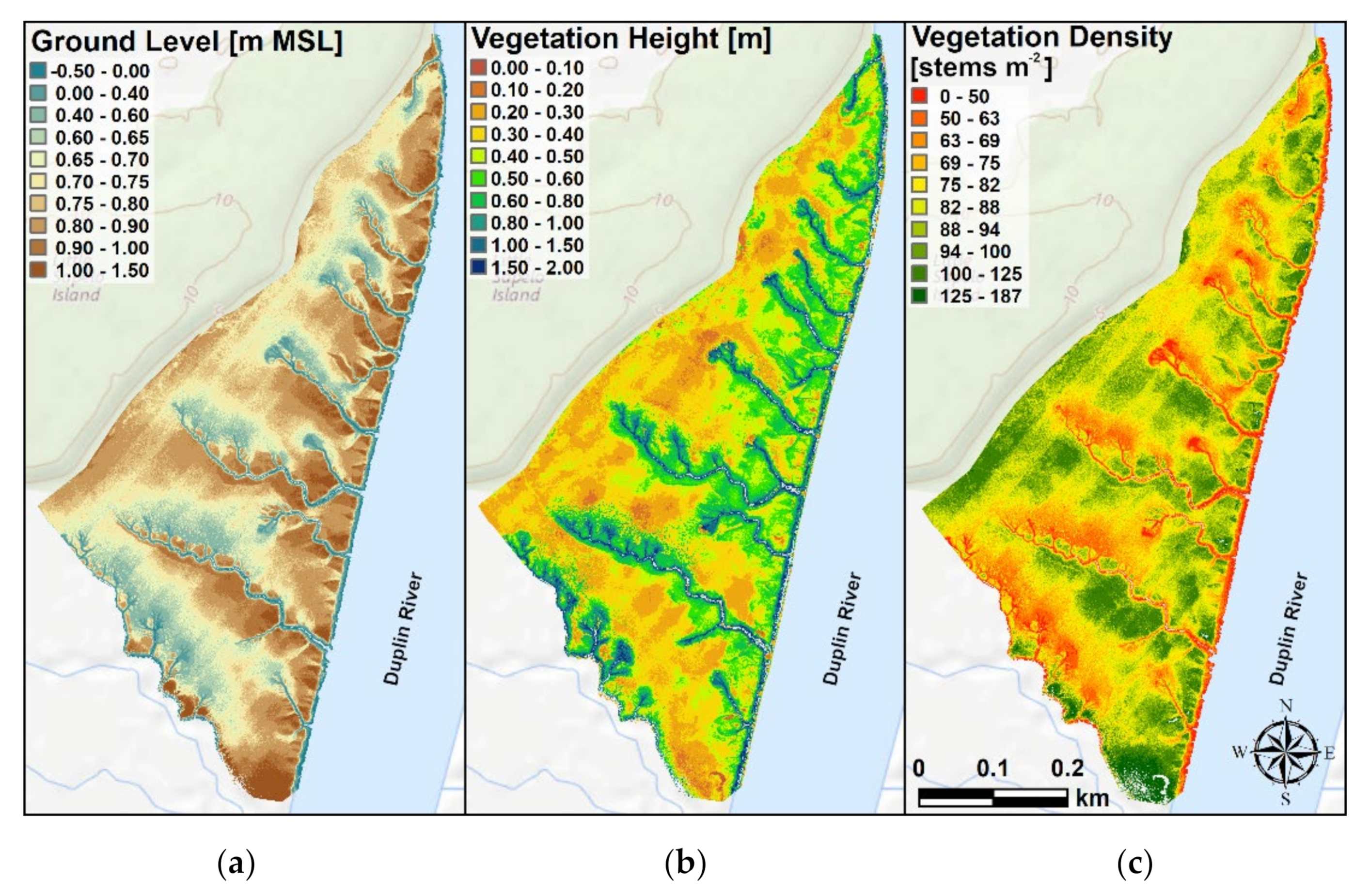
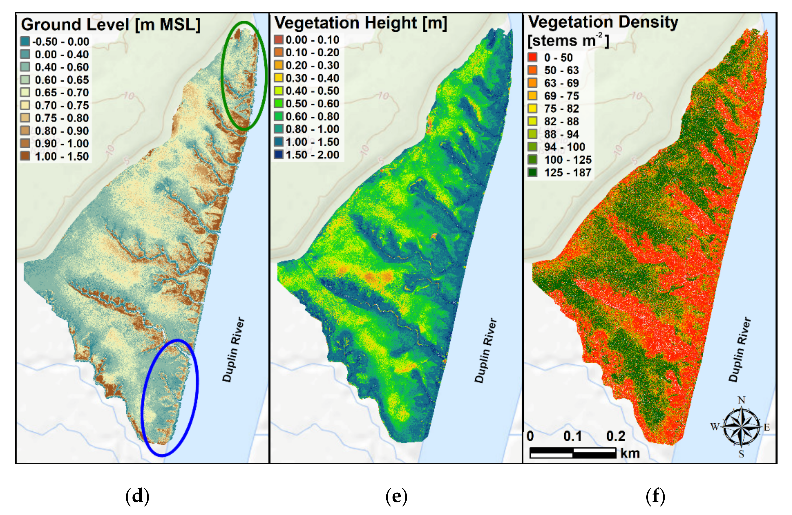
Finally, we determined the spatial distribution (maps/DEMs) of ground elevation and vegetation characteristics (height and density) by applying Equations (9), and (11)–(14) to the cells of the study area. Figure 5 shows the maps obtained from the LiDAR (first row) and the DAP-UAV (second row) point clouds.

4. Discussion

4.1. Ground Elevation Estimate

This study evaluates the skills of two types of drone-based point clouds, derived with LiDAR and DAP-UAV techniques, in estimating ground elevation. The point clouds are transformed using the regression plane method proposed in Pinton et al. (2020) [23]. For a comparative purpose, the ground elevation is computed on both the transformed and non-transformed point clouds.
The results of the linear regression (9) applied to the LiDAR-UAV and DAP-UAV datasets (Table 3 and Figure 3) underline that, when the transformation method is applied, the ground elevation estimates change from underestimated to slightly overestimated, independently on the collection method of the point cloud. The overestimation is due to the dense vegetation populating the area. For DAP-UAV, this vegetation limits the identification of the same ground location in consecutive high-resolution images, restricting the construction of the point cloud on the upper part of the vegetation layer (Figure 6a). However, in some of the surveyed plots, we observed a relative underestimation of the ground elevation obtained from the point cloud (Figure 6b; Figure 7g,h). This could be related to: (i) possible distortions of the images, due to significant movements of the UAV, caused by sudden wind gusts; (ii) imprecise identification of the GCPs by the Pix4D software, caused by glares or shadows on the images; (iii) insufficient number of GCPs at the boundary of the study domain. The results reported in Figure 3c,d show that many points, placed between 0.60 and 0.80 m, present a very good agreement between surveyed and calculated ground elevation. These points generally represent low-vegetated areas on the marsh platform, where the ground, and consequently its elevation, could be easily identified in the collected images. Finally, Figure 6c shows that the LiDAR-UAV point cloud accurately captures the real ground elevation, as well as the mean and maximum vegetation height (see Section 3.1 and Section 3.2 for more details), thus facilitating their identification.
The value of the evaluation metrics in Table 2 shows that: (i) LiDAR-UAV point clouds have higher predictive skills than the DAP-UAV dataset in determining the ground elevation. This is true for both the original (non-transformed) point cloud and the point cloud transformed by using the regression plane method. (ii) For the LiDAR-UAV dataset, when using the transformed point cloud errors reduce over the entire domain, particularly for the creek samples, owing to the larger slopes. (iii) For the DAP-UAV point cloud, the errors are on average unchanged when the point cloud is transformed, thus indicating that the method does not improve or reduce the estimates obtained from this point cloud.
In conclusion, the results underline the superiority of LiDAR-UAV over DAP-UAV in computing the bed elevation on a vegetated salt marsh.

4.2. Vegetation Height and Density Estimate

Equations (11)–(14) summarize the results obtained by the genetic algorithm. Equations (11), (12) and (14) underline the importance of σ n , e , that represents the vertical spreading of the local point cloud, for the description of the vegetation characteristics. To our knowledge, this is the first time σ n , e was used to estimate vegetation height. In previous studies, vegetation height was preferentially estimated using the maximum ( z n , e m a x ) [53,55,99,100,101,102] or mean ( z n , e m e a n ) [92] point cloud height, as we did in Equation (13). The reason is the lower resolution of their point clouds, in comparison with the one we used in this study, which makes it difficult to describe the local standard deviation of the point’s elevation.
The formulation we obtain to calculate the vegetation height from the DAP-UAV point cloud (Equation (13)) differs from the one obtained by Pinton et al. (2020) [23] using the LiDAR-UAV dataset (Equation (11)). According to Equation (13), tall vegetation is observed for high values of the mean elevation of the transformed point cloud ( z n , e m e a n ). This is because the mean elevation, calculated with respect to the local minimum, is approximately half of the vegetation height. Equation (13) also indicates that tall vegetation is associated with low values of the local minimum green index value ( G n , e m i n ). This is appropriate considering that low values of the Green-band indexes refer to darker pixels, which are usually associated with tall vegetation. The presence of the predictor G n , e m i n in the equation suggests the inability of the DAP-UAV dataset to correctly predict the vegetation height if not coupled with an auxiliary dataset.
To estimate the vegetation density, the GA gives partially different equations for the LiDAR- and DAP-UAV datasets (Equations (12) and (14), respectively). Both equations depend on the same predictor σ n , e , with slightly different coefficients. The variance has a lower importance for the DAP-UAV dataset. The coefficient reduces from 0.39 to 0.174. According to Equation (14), vegetation density increases with the skewness ( S n , e ) of the DAP-UAV point cloud distribution. This is likely due to the lower penetration of DAP-UAV with higher densities. The skewness, in fact, reduces in value in tall vegetation areas, because most of the points are obtained on the upper part of the vegetation layer. In Equation (12), the predictor z n , e m e d i a n is preferred to S n , e . As for S n , e , the median elevation, calculated with respect to the ground, reduces for low density vegetation, because most of the points detected by the laser scanner hit the marsh bed. The importance of this second parameter is higher for the DAP-UAV dataset. The coefficient increases from 0.39 to 0.784.
With this study, we examine the possible advantage of coupling UAV-based point clouds and RGB datasets to compute vegetation height and density. Usually, point clouds are coupled with imagery datasets, such as RGB data, to perform land cover analysis and classification, and for vegetation mapping [53,54,55]. This coupling is in some cases necessary for airborne [53,55,98,103] and UAV [104] point clouds to improve the estimates of vegetation characteristics, due to the low classification skills related to the low point-cloud resolution. Moffett and Gorelick (2013) [54] investigated the effect of coupling airborne LiDAR point clouds to RGB datasets for vegetation classification, discouraging the use of LiDAR datasets alone. In particular, they obtained the smallest estimation error by using only imagery datasets, due to the LiDAR resolution being smaller (~1 m) than the RGB resolution (0.30 m). This suggests that adding a point-cloud dataset is beneficial for classification purposes only if its resolution is similar or higher than the resolution of the initial dataset. Our results confirm this outcome. The estimates computed using LiDAR- and LiDAR-UAV plus RGB predictors have similar accuracy, due to the high density of the LiDAR-UAV dataset. On the contrary, the classification performances of the DAP-UAV predictors increase when coupled with the RGB predictors, because of the low density of the point cloud (Figure 6).
In conclusion, we showed the superiority of LiDAR-UAV over DAP-UAV in computing vegetation characteristics on a salt marsh. Moreover, we showed that when RGB data are coupled with LiDAR-UAV data, RGB does not improve the classification skills of the point cloud alone in computing vegetation height and density on a salt marsh. Therefore, we suggest to use LiDAR datasets alone for wetland mapping purposes and to avoid the additional effort of collecting and processing RGB data.

4.3. High-Resolution Maps: LiDAR-UAV vs. DAP-UAV

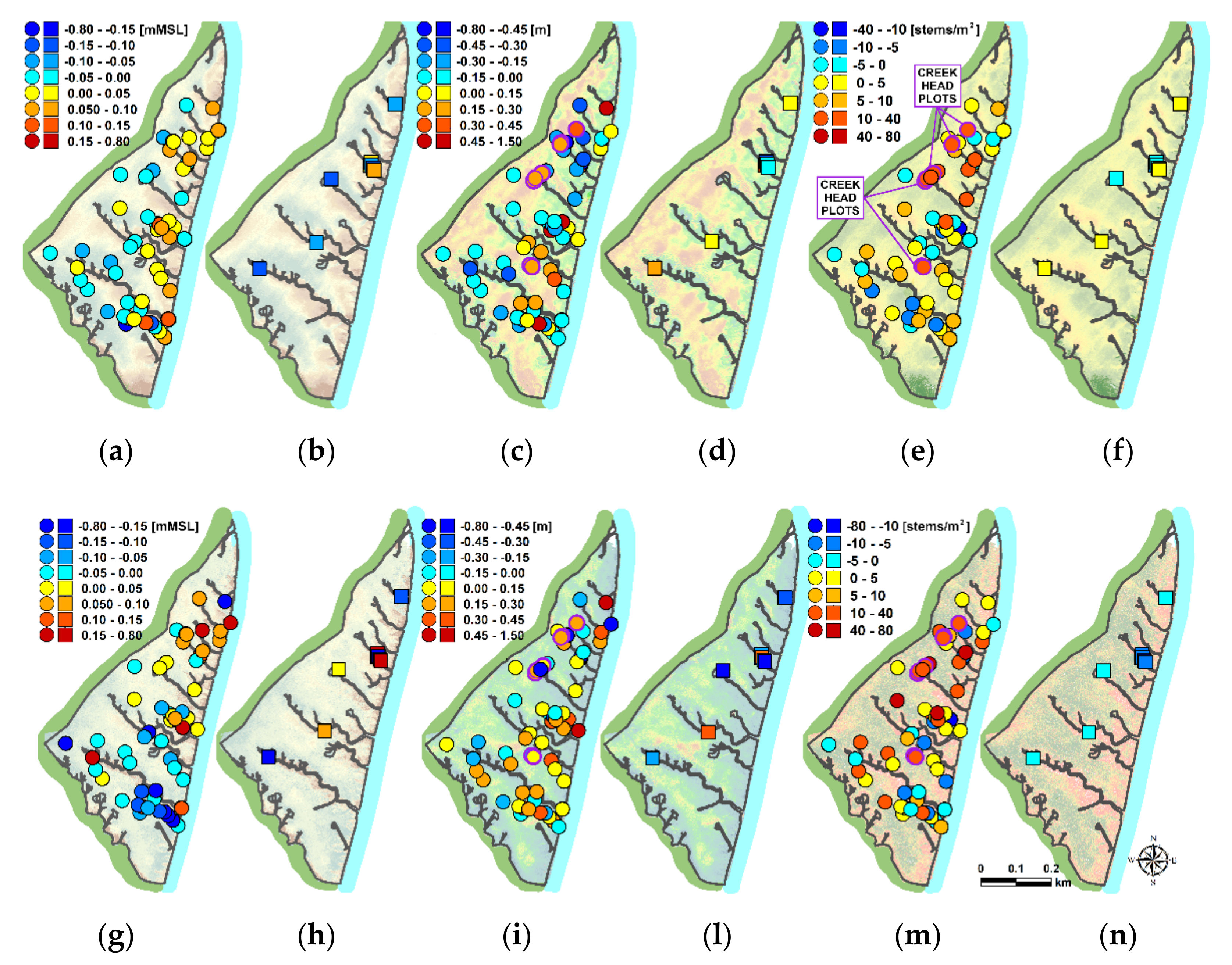
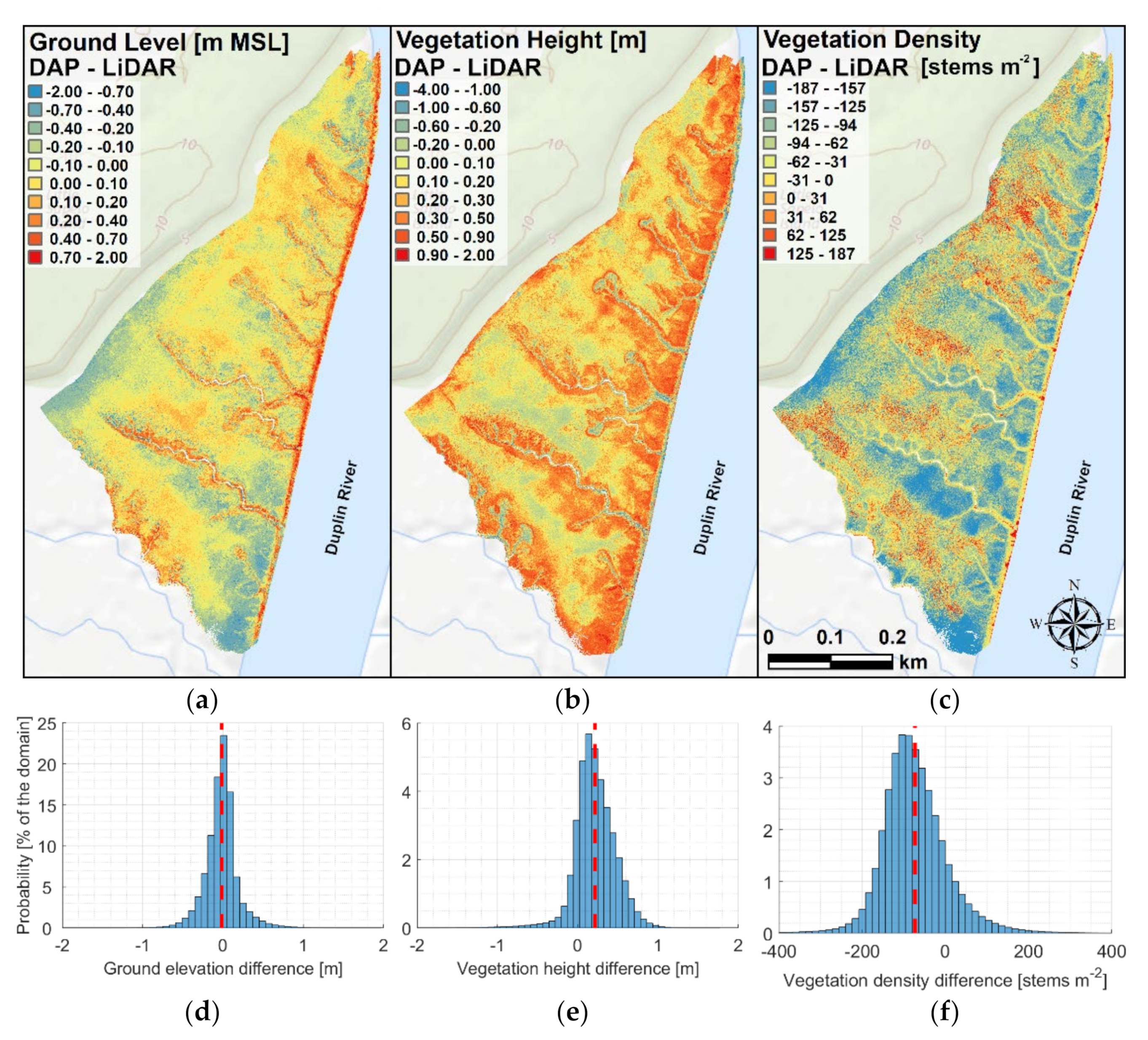
We can visually compare the spatial distribution of ground elevation, vegetation height, and vegetation density in the salt marsh, obtained from the LiDAR (first row) and DAP-UAV (second row) datasets by using the high-resolution maps in Figure 5. Results show notable differences between the distributions. From Figure 7 instead, we can visualize the estimation error for the ground elevation (Figure 7a,b,g,h), vegetation height (Figure 7c,d,i,l), and vegetation density (Figure 7e,f,m,n), calculated on the plots surveyed on the marsh platform (circles) and the tidal creeks (squares) by using the LiDAR- (first row) and the DAP-UAV (second row) point clouds. Figure 8 shows the spatial distribution (first row), and the frequency distributions (second row) of the ground elevation, vegetation height, and vegetation density differences between the DAP- and LiDAR-UAV-based maps.
From the spatial distribution of ground elevation computed with both the LiDAR and DAP-UAV point clouds (Figure 5a,d), we observe that high-elevation areas are located at the marsh edge and the creek levees. In addition, from the LiDAR-UAV-based map (Figure 5a), we observed that the elevation progressively reduces in the marsh platform and reaches minimum values at the south-western side of the creeks. This suggests a preferential sediment deposition, due to tidal fluxes in which the cross-creek component goes from north-east to south-west [19]. The difference between the two sides of the creeks is less marked in the DAP-UAV-based map (Figure 5d), which shows lower elevations in the southern side of the channels (~0.50–0.80 m MSL), in comparison with the LiDAR (~0.70–1.00 m MSL), and similar values on the northern side. This is due to the higher underestimation errors observed in the southern side of the creeks for the DAP-UAV dataset (−0.05–0.80 m, Figure 7a), in comparison with LiDAR-UAV, which instead shows low overestimation errors (−0.05–0.10 m, Figure 7g). These differences are more marked for the creeks placed in the southern portion of the study domain. In addition, the DAP-UAV map shows higher ground elevations on the creek levees and the marsh edge (~1.00–1.50 m MSL), than the LiDAR-UAV map (~0.90–1.05 m MSL). This is due to the higher overestimation observed in most of the plots placed on the creeks for the DAP dataset (0.00–1.50 m), in comparison with the LiDAR-UAV one (0.15–0.30 m). Finally, Figure 5a,d show comparable results on the marsh platform, as confirmed by the comparable errors reported in Figure 7a,g for these areas. However, the spatial distribution obtained from the LiDAR is smoother, and thus better represents the real shape of the marsh platform. Moreover, the DAP-UAV point cloud gives a rougher ground shape in the areas where the vegetation changes rapidly (i.e., between high and medium vegetation, and close to the creeks). Here, the calculated ground elevation changes suddenly (~1.05–1.50 m MSL to ~0.50–0.70 m MSL), due to the low penetration of the DAP-UAV in the vegetation (see Figure 6 and Section 3.1), thus creating a step. This step is not visible in the LiDAR-UAV-based results due to the higher penetration of this survey technique in the vegetation layer. The results in Figure 8a confirm that DAP gives high ground levels on the creek levees and the marsh edge, due to the low penetration of the DAP-UAV point cloud in the dense vegetation layer covering these two areas. The high values observed at the edge may be due to an additional effect of the local slope.
Considering these results, we can assume that the differences between the two datasets increase with the vegetation height, because of the different penetration skills of the two datasets in the vegetation layer. Thus, the ground elevation obtained from the DAP- and LiDAR-UAV has similar values in most of the low-vegetated marsh. Figure 8d confirms this result, indicating that in ~50% of the marsh, the ground elevation difference is between ±10 cm.
In addition, DAP-UAV provides smaller values of marsh elevation than LiDAR-UAV on the south-eastern (blue circle in Figure 5d) and the northern edge of the marsh (green circle in Figure 5d). These erroneous results are probably due to georeferentiation errors. The images collected in these areas are located at the boundary of the domain. The number of GCPs visible in these images is limited due to the presence of the Duplin River (south) and the freshwater forest (north). On the contrary, the LiDAR-UAV does not rely on GCP for georeferencing the cloud, but on the Inertial Measurement Unit and the GNSS receiver, both mounted on the airframe, as well as on the local base station and the service OPUS, used to correct the data from the GNSS (Section 2.3). This system ensures a precise and homogeneous georectification of the LiDAR-UAV dataset in the surveyed domain. The results in Figure 8a indicates that in the northern and southern boundaries of the marsh, the DAP-UAV point cloud estimates lower ground elevation than the LiDAR-UAV point cloud. The same is observed at the western boundary of the study area. This is due to the small number of GCPs in that area, and the possible interference of the local freshwater forest. In addition, we observed that the distribution in Figure 8d is slightly skewed toward negative values (skewness = 0.208), and has a mean value of −0.018 m.
From Figure 5b, we observed that the Spartina alterniflora distribution obtained from the LiDAR-UAV point cloud is consistent with the distribution usually observed in salt marshes [89,90,105,106]. Tall Spartina alterniflora preferentially occupies the creeks, the marsh edge, and their adjacent areas, where the bed elevation is higher, the hydroperiod increases, and the salinity impact is lower. The vegetation height on the levees ranges between 1.00 and 1.80 m, and progressively decreases away from the creek, reaching ~0.20 m on the marsh platform, where the hydroperiod is lower and salinity is higher [89]. While the same distribution is obtained for the DAP-UAV point cloud, the values are generally higher (Figure 5e). In particular, vegetation height is unlikely close to ~0.60–0.80 m almost everywhere in the marsh platform, and ~1.50–2.00 m on a large area adjacent to the creek levees and the marsh edge. This is because, while the DAP-UAV dataset largely overestimates vegetation height in the marsh platform, the LiDAR-UAV dataset slightly underestimates it, as reported in Figure 7c,i. For the LiDAR-UAV dataset, high overestimation is generally observed at the non-vegetated creek heads (purple-bounded dots in Figure 7). Here, the model predicts a vegetation height of ~0.15–0.45 m. This is probably due to the proximity of high-vegetated areas, whose point cloud is partially used to compute the vegetation height, and to the similarity of these areas with the low-vegetated marsh. In addition, the results reported in Figure 7d,l show that the estimation errors, both positive and negative, calculated on the plots on the creeks, are higher for the DAP-UAV than for the LiDAR-UAV dataset. Finally, notice that both LiDAR-UAV and DAP-UAV distributions correctly show higher values of vegetation height over the mussel mounds, in comparison with the adjacent area.
The results in Figure 8b underline that, compared to LiDAR, DAP preferentially estimates higher vegetation height in the marsh system. This happens in ~85% of the marsh system, as indicated in Figure 8e. High positive differences, which can reach 2 m, are observed close to the creeks and the marsh edge. Low negative differences are observed in the low-vegetated marsh platform, and high negative differences are observed at the unvegetated creek heads. The distribution in Figure 8e is asymmetrical and skewed toward positive values (skewness = −0.847), and has a mean value of 0.215 m.
Using a LiDAR point cloud (Figure 5c), we observed that vegetation density is higher where vegetation is not tall. Conversely, low vegetation densities were calculated in conjunction with tall vegetation, on the creek levees, the creek heads, and on the marsh edge. The results reported in Figure 7e,m indicate that the DAP-UAV overestimates the vegetation density in the marsh platform (Figure 7m) more and more frequently than LiDAR-UAV does (Figure 7e). The results reported in Figure 7f,n indicate that while DAP-UAV underestimates vegetation density at the creeks (−5–10 stems m−2), LiDAR slightly overestimates it (0–5 stems m−2). The overestimation observed for the DAP-UAV dataset at the marsh platform depends on the low value of Δ z n , e estimated by the point cloud in this area, which increases the estimate of the vegetation density from Equation (10). Conversely, the underestimation with DAP-UAV dataset on the creeks, and in the adjacent area, depends on the high value of Δ z n , e estimated there, which reduces the value of the vegetation density obtained from Equation (10). In addition, both datasets overestimate the density at the creek head (purple-bounded dots in Figure 7), because of the similarity of these areas with the low-vegetated marsh (0–5 stems m−2).
The results reported in Figure 8c underline that, compared to LiDAR, DAP preferentially estimates lower vegetation density in the marsh system. This happens in ~85% of the marsh system, as indicated in Figure 8f. Negative differences are generally observed close to the creeks and the marsh edge, where Spartina alterniflora is tall or medium, and positive differences are observed especially at the creek heads. The distribution observed in Figure 8f is asymmetrical and skewed toward negative values (skewness = 0.587) and has a mean value of −73.00 stems m−2.

4.4. Point Cloud Accuracy in the Literature

As indicated in the method section, we calculated the RMSE georeferencing values of our 27 GCPs, for both the LiDAR- and the DAP-UAV point clouds. The horizontal and vertical RMSE of the GPS measurements correspond to 0.023 and 0.062 m for the LiDAR-UAV point cloud, and 0.050 and 0.104 m for the DAP-UAV point cloud. For the DAP-UAV dataset, the errors are comparable with the ones observed in other studies, using similar UAVs, whose values are reported in Table 5.

4.5. Limits of the Method

The following is a list of the limitations affecting our method. In addition, we reported how to bypass them:
  • Although our method detects vegetation characteristics remotely from a UAV, it requires active walking on the marsh to (i) position the land station used to calibrate the GNSS sensor on the drone, and (ii) survey bed elevations, vegetation height, and vegetation density, for calibration and validation purposes. The first limitation can be reduced by positioning the station at the boundary of the survey area, limiting the trampling to a very restricted area of the marsh. The second limit could be only partially bypassed by surveying ground elevation from a boat or a kayak, at the high tide. This method could not be used to survey vegetation properties because most of it is completely submerged during high tide. In conclusion, because this limitation could not be completely bypassed, its effects can be reduced by reducing the number of surveyed plots. Future research may be conducted to determine the error obtained by using datasets of different sizes and compositions to calibrate and validate our model.
  • Due to the inability of our LiDAR sensor to collect data underwater, our approach is not used to determine the ground level and the vegetation characteristics in subtidal coastal areas. This is the reason for the missing outputs in Figure 5. The missing values correspond to the portion of the creeks close to the main channel, where water is present even at low tide. This limitation could be bypassed by using dual-frequency laser scanners, which allow the detection of both topography and (underwater) bathymetry [110,111]. Especially in the main channel, where the water turbidity could reduce the performances of these dual-frequency LiDAR, the survey can be done by using Unmanned Underwater Vehicles (UUV). However, this technology is more expensive than the one used in standard topographic laser scanners, and their precision depends on water turbidity, which is generally high in our study area.
  • The short (~20–30 minutes) battery life of the aircraft limits the usage of the method to relatively small areas. This limitation can be bypassed by using surrogate aircraft, such as ultralight aircraft. However, the use of these aircraft (i) requires adequate landing and take-off areas, such as an airport, reducing the flexibility of the survey obtained with vertical take-off and landing (VTOL) UAVs; (ii) is less stable than VTOL UAVs, thus complicating dataset collection and post-processing steps; (iii) requires human personal onboard, nullifying the reduction of human loss risk obtained using UAVs.
  • A LiDAR survey requires the presence of a licensed and expert drone pilot to be performed, and the use of an adequate acquisition system (i.e., laser scanner). However, due to the great popularity drones are gaining in many fields, pilots’ availability is increasing, and the cost to recreate an acquisition system similar to the one we used is becoming more affordable.

5. Conclusions

In this study, we evaluate the possibility to estimate ground elevation and vegetation characteristics in a highly vegetated salt marsh system, using UAV-based DAP point clouds. The point cloud is also coupled with an imagery (RGB) dataset to verify its impact on algorithm estimates. To estimate ground elevation and vegetation characteristics, we employ the method proposed by Pinton et al. (2020). Results are validated using a robust LOOCV method and compared with the results obtained in our previous study by using a UAV-LiDAR point cloud.
Our study is the first one comparing the performances DAP- and LiDAR-UAV point clouds when they are used to describe topographic and vegetation features in a salt marsh system. Previous studies perform this comparison mainly in the forestal area. The results we obtained underline the pro and cons of DAP- and LiDAR-UAV methods in this environment, and for this reason, can help both scientists and local managers to choose the best survey methods based on their budget and the quality of their outcomes. While SfM datasets would appeal to users with a low budget and with a need for “ballpark” estimates, LiDAR-UAV data would appeal to users with a higher budget and an interest in high-accuracy data. Because LiDAR sensors are already being fully integrated with RGB cameras, the collection of both datasets is becoming every day more common. However, the capability to collect both datasets will be restricted only to high-cost applications.
The model outputs suggest that, while for the LiDAR-UAV point cloud the regression plane approach reduces the error introduced by non-flat ground computing ground elevation and vegetation characteristics, the error remains on average unchanged for the DAP-UAV point cloud. Moreover, due to the high penetration of the laser scanners in vegetation, LiDAR-UAV captures the large gradients of the computed variables and the vegetation characteristics, close to tidal creeks and where vegetation is tall and dense, better than DAP-UAV.
The results (Table 4 and Table 5) indicate that the accuracy of the classification procedure notably improves when RGB images are used as input parameters together with the DAP-UAV point cloud. Thus, we discourage using DAP-UAV point clouds for high-resolution vegetation mapping of coastal areas if not coupled with other data sources. Conversely, the results indicate that the accuracy of the classification procedure negligibly improves when RGB images are used as input parameters together with the LiDAR point cloud. Thus, in this case, the limited reduction in the estimation error does not justify the collection and analysis of the RGB dataset. Moreover, the classification is more accurate by using the LiDAR-UAV than the DAP-UAV dataset. The result does not change if the datasets are coupled with the RGB images. Thus, we encourage the use of LiDAR-UAV instead of DAP-UAV to map tidal wetlands.
With the present research, we show that our algorithm should be recalibrated if used with point clouds collected with different techniques, even in the same location. This assumption will likely hold for surveys performed for different locations, grass species, and seasons. A correct recalibration of the GA needs a dataset of 50–100 vegetation samples to be successful. However, we do not exclude the possibility to avoid the recalibration of the algorithm when it is used for similar locations and vegetation properties, and with the same collection technique.
Our method can be used to evaluate the temporal variation in vegetation characteristics and distribution in a coastal area. This aim can be achieved by acquiring point clouds in the same area periodically, by maintaining unchanged the survey technique and specifics. Periodic remote sensing surveys can be also used to quantify the effects of droughts, and extreme events (i.e., hurricanes and storms) on marsh morphology and vegetation. This application related to extreme events requires the knowledge of where and when an extreme event will hit the coastline, which is predictable with adequate precision only in the short-term period. Due to the flexibility of the UAV surveys, they can be performed in the short time frame preceding the hazardous event, avoiding the adverse meteorological conditions that accompany these events, and consequently, the risks for both the airframe and the survey team. In addition, this aim requires a survey on the area immediately after the hazardous event, which is generally feasible. Our method can also be used to evaluate marsh vertical accretion due to organic and inorganic deposition in the long term. Finally, the method presented in this study can be applied to other coastal systems to evaluate ground elevation and vegetation characteristics. Our research interest is currently focusing on coastal dunes.
Numerical models are generally used in coastal applications to quantify the transport of nutrients, pollutants, and sediments. Sediments, in particular, are used to estimate the morphological changes of coastal environments in the short-, medium-, and long-term periods. Typically, such models are initialized with a time-invariant roughness, which is calibrated using a sensitivity analysis and is then uniformly applied to the domain. Some approaches, consider a nonuniform roughness and base it on the distribution of vegetation height, stem diameter, density, biomass, or submergence rate over the domain. Considering that spatial variations in vegetation characteristics modulate frictional resistance, modifying the local hydrodynamics and morphodynamics, the predictive abilities of such models will benefit from a truthful spatial description of the vegetation. With our method, we can provide both vegetation and topographic data at high resolution by using UAV-based surveys, thus favoring model calibration.
Future works will focus on applying the point cloud transformation algorithm to other coastal environments, with different ground shapes and vegetation typologies, such as coastal dunes, and the freshwater forests bounding both salt marshes and dunes environments. For instance, tracking freshwater forest landward migration can be used as a proxy to estimate saltwater intrusion in the salt marshes, which is an indicator of coastal threat due to SLR. In addition, tracking the evolution of tidal creeks in a marsh environment can be beneficial to forecast future changes in the marsh hydrodynamic, which can influence the local topography, the vegetation patterns, and the distribution and behavior of local communities, such as ribbed mussels, which become more popular due to their contribution to marsh accretion. Moreover, additional studies can be done to evaluate the performances of different machine learning techniques when they are used to estimate ground elevation and vegetation characteristics in a coastal environment from high-resolution point clouds. This can be useful to understand if different algorithms can provide better results for different vegetation patterns and typologies, consequently helping scientists and data analysts to choose the algorithm maximizing the quality of their results.
Finally, additional studies can be performed to evaluate the effect of flight altitude on LiDAR- and DAP-UAV point cloud penetration in the dense vegetation layer covering the salt marsh. Penetration could be described by using a Canopy Cover index. Because Canopy Cover is not commonly used in salt marsh environments, a standardized method to describe it will have to be determined. Future studies should focus on identifying the flight altitude which minimizes the estimation error for ground elevation, vegetation height, vegetation density, and aboveground biomass obtained from both LiDAR- and DAP-UAV point clouds.

Author Contributions

Conceptualization, D.P. and A.C.; methodology, D.P. and A.C.; software, D.P.; validation, D.P.; formal analysis, D.P.; investigation, D.P. and A.C.; resources, A.C., B.W. and P.I.; data curation, D.P., B.W., P.I. and A.O.; writing—original draft preparation, D.P. and A.C.; writing—review and editing, D.P. and A.C.; visualization, D.P.; supervision, A.C.; project administration, D.P. and A.C.; funding acquisition, A.C. All authors have read and agreed to the published version of the manuscript.

Funding

Pinton was supported by the UF SEED (P0081941) and by the UF “Moonshot” (No. 00129098) awards.

Institutional Review Board Statement

Not applicable.

Informed Consent Statement

Not applicable.

Data Availability Statement

Not applicable.

Acknowledgments

Authors want to thank the University of Georgia Marine Institute, Ike Sellers, and Gracie Townsend, Christine Angelini who allowed us to use her boat for the fieldwork, and Collin Ortals for his contribution to the fieldwork. This research was supported by the UF Informatics Institute and the UF One Health Center of Excellence fellowship programs.

Conflicts of Interest

There is no conflict of interest related to this paper.

Appendix A

Here, we report the steps of the point cloud transformation algorithm proposed in Pinton et al. (2020) [23].
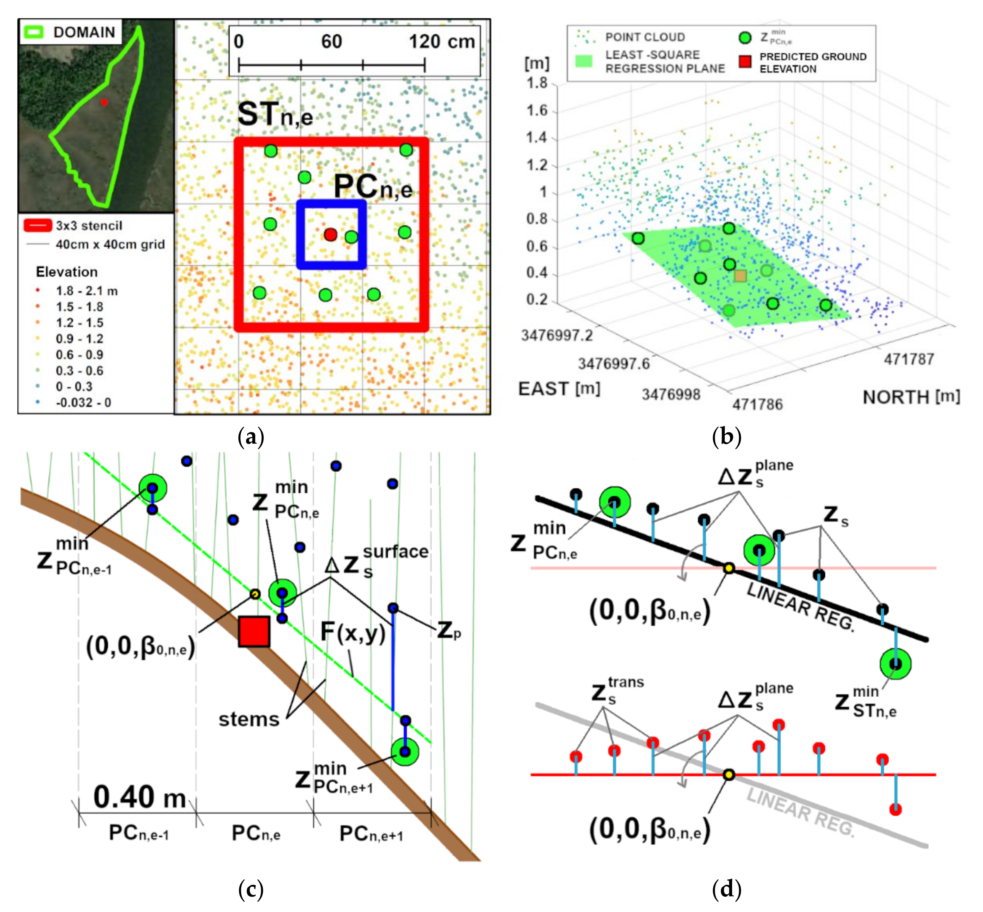
STEP 1: The point cloud is split into subsets (PCn,e, Figure A1a), which are contained in the 0.40 m × 0.40 m regular cells (n,e) constituting the regular grid that covers the entire study domain.
STEP 2: For each cell (n,e), the elevation of the lowest point (green dots, Figure A1) of the related subset PCn,e is calculated as:
z   P C n , e m i n = min   p P C n , e z p   ,
where z p is the elevation of the generic point p belonging to the subset PCn,e.
STEP 3: The coordinates of the lowest points (green dots, Figure A1) of the nine cells constituting STn,e are used to define a least-squares regression plane F x , y   (green plane, Figure A1b). The surface reads:
F x , y = β 0 , n , e + β x , n , e   x + β y , n , e   y   ,
where β 0 , n , e is the intercept of the plane with a vertical axis passing for the midpoint of the stencil, and β x , n , e and β y , n , e are the regression coefficients of the plane. They represent the eastward and northward slopes of the regression plane, respectively.
STEP 4: The vertical distance ( Δ z s s u r f a c e , blue vertical lines, Figure A1c) between the regression plane and the points of the point cloud contained in STn,e is calculated as:
Δ z s s u r f a c e = z s F x s , y s s S T n , e   ,
where x s , y s , and z s are the coordinates of the s t h point of the point cloud. The origin of the horizontal coordinates ( x s , y s ) is the midpoint of STn,e.
STEP 5: For each STn,e, the transformed point cloud (Figure A1d) is obtained by summing Δ z s s u r f a c e , that was calculated for each point at STEP 4, to β 0 , n , e , which is the intercept of the regression plane with a vertical axis passing for the midpoint of the stencil. The elevation of each point “s” ( z s t r a n s ) is obtained as:
z s t r a n s = β 0 , n , e + Δ z s s u r f a c e   ,
STEP 6: The elevation of the lowest point of the transformed point cloud ( z   S T n , e m i n ) in STn,e is identified as:
z   S T n , e m i n   =   min   s S T n , e z s t r a n s   .
Finally, the relative elevation ( z s r e l ) of the sth point of the transformed point cloud with respect to the lowest point in STn,e ( z   S T n , e m i n ) is obtained as follows:
z s r e l   =   z s t r a n s z   S T n , e m i n   .
Figure A1. The image reports the steps of the procedure used to transform the point cloud and calculate the ground elevation on a specific cell (n,e). (a) The point cloud is split using a regular grid (STEP 1), and the elevation of the lowest point in each (n,e) cell (green dots) is calculated (STEP 2). (b) The lowest points (green dots) of the cells belonging to a stencil (STn,e) are used to determine a regression plane (STEP 3). (c) The vertical distance ( Δ z s s u r f a c e ) between the regression plane and each point (s) of the point cloud contained in STn,e is calculated (STEP 4). (d) The point cloud contained in STn,e is transformed (red points) and the relative elevation ( z s t r a n s ) of the points is calculated, using as reference the elevation of the lowest transformed point in STn,e (STEP 5). The elevation of the lowest point is used as the best estimate of the ground elevation in the central cell of the stencil (STEP 6). STEPs 4–6 are reported in 2D, for clarity. (Adapted from Pinton et al. (2020)).
Remotesensing 13 04506 g0a1

References

  1. Pinton, D.; Xu, S.; Canestrelli, A. Managing Dyke Retreat: Importance of Channel Network Evolution and Mainland Slope on Storm Surge Dissipation Over Salt Marshes. AGU Fall Meeting 2020, 2020, EP061-0016. [Google Scholar]
  2. Stark, J.; Van Oyen, T.; Meire, P.; Temmerman, S. Observations of tidal and storm surge attenuation in a large tidal marsh. Limnol. Oceanogr. 2015, 60, 1371–1381. [Google Scholar] [CrossRef]
  3. Boesch, D.F.; Turner, R.E. Dependence of Fishery Species on Salt Marshes: The Role of Food and Refuge. Estuaries 1984, 7, 460–468. [Google Scholar] [CrossRef]
  4. Barbier, E.B.; Hacker, S.D.; Kennedy, C.; Koch, E.W.; Stier, A.; Silliman, B. The value of estuarine and coastal ecosystem services. Ecol. Monogr. 2011, 81, 169–193. [Google Scholar] [CrossRef]
  5. Pendleton, L.; Donato, D.C.; Murray, B.C.; Crooks, S.; Jenkins, W.A.; Sifleet, S.; Craft, C.B.; Fourqurean, J.; Kauffman, J.B.; Marbà, N.; et al. Estimating Global “Blue Carbon” Emissions from Conversion and Degradation of Vegetated Coastal Ecosystems. PLoS ONE 2012, 7, e43542. [Google Scholar] [CrossRef] [Green Version]
  6. Hardisky, M.A.; Gross, M.F.; Klemas, V. Remote Sensing of Coastal Wetlands. BioScience 1986, 36, 453–460. [Google Scholar] [CrossRef]
  7. Alizad, K.; Hagen, S.C.; Medeiros, S.C.; Bilskie, M.V.; Morris, J.T.; Balthis, L.; Buckel, C.A. Dynamic responses and implications to coastal wetlands and the surrounding regions under sea level rise. PLoS ONE 2018, 13, e0205176. [Google Scholar] [CrossRef]
  8. Day, J.W.; Kemp, G.P.; Reed, D.J.; Cahoon, D.R.; Boumans, R.M.; Suhayda, J.M.; Gambrell, R. Vegetation death and rapid loss of surface elevation in two contrasting Mississippi delta salt marshes: The role of sedimentation, autocompaction and sea-level rise. Ecol. Eng. 2011, 37, 229–240. [Google Scholar] [CrossRef]
  9. Morris, J.; Sundberg, K.; Hopkinson, C. Salt Marsh Primary Production and Its Responses to Relative Sea Level and Nutrients in Estuaries at Plum Island, Massachusetts, and North Inlet, South Carolina, USA. Oceanography 2013, 26, 78–84. [Google Scholar] [CrossRef]
  10. Kirwan, M.L.; Temmerman, S.; Skeehan, M.L.K.E.E.; Guntenspergen, G.R.; Fagherazzi, S. Overestimation of marsh vulnerability to sea level rise. Nat. Clim. Chang. 2016, 6, 253–260. [Google Scholar] [CrossRef]
  11. Saintilan, N.; Kovalenko, K.; Guntenspergen, G.; Rogers, K.; Lynch, J.; Cahoon, D.; Gamage, V.P. Global patterns and drivers of tidal marsh response to accelerating sea-level rise. Res. Sq. 2021. in review. [Google Scholar] [CrossRef]
  12. Mahdianpari, M.; Granger, J.E.; Mohammadimanesh, F.; Warren, S.; Puestow, T.; Salehi, B.; Brisco, B. Smart solutions for smart cities: Urban wetland mapping using very-high resolution satellite imagery and airborne LiDAR data in the City of St. John’s, NL, Canada. J. Environ. Manag. 2020, 280, 111676. [Google Scholar] [CrossRef] [PubMed]
  13. US Census Bureau. Coastline America No. June. 2019. Available online: https://www.census.gov/library/visualizations/2019/demo/coastline-america.html (accessed on 7 November 2020).
  14. Marani, M.; Belluco, E.; D’Alpaos, A.; Defina, A.; Lanzoni, S.; Rinaldo, A. On the drainage density of tidal networks. Water Resour. Res. 2003, 39, 1040. [Google Scholar] [CrossRef]
  15. Reed, D.J.; Cahoon, D.R. The relationship between marsh surface topography, hydroperiod, and growth of Spartina alterniflora in a deteriorating Louisiana salt marsh. J. Coast. Res. 1992, 8, 77–87. [Google Scholar]
  16. Beeson, C.; Doyle, P.F. Comparison of bank erosion at vegetated and non-vegetated channel bends. JAWRA J. Am. Water Resour. Assoc. 1995, 31, 983–990. [Google Scholar] [CrossRef]
  17. Peruzzo, P.; Viero, D.P.; Defina, A. A semi-empirical model to predict the probability of capture of buoyant particles by a cylindrical collector through capillarity. Adv. Water Resour. 2016, 97, 168–174. [Google Scholar] [CrossRef]
  18. Fagherazzi, S.; Kirwan, M.L.; Mudd, S.M.; Guntenspergen, G.T.; Temmerman, S.; D’Alpaos, A.; van de Koppel, J.; Rybczyk, J.M.; Reyes, E.; Craft, C.; et al. Numerical models of salt marsh evolution: Ecological, geomorphic, and climatic factors. Rev. Geophys. 2012, 50, RG1002. [Google Scholar] [CrossRef]
  19. Pinton, D.; Canestrelli, A.; Fantuzzi, L. A UAV-Based Dye-Tracking Technique to Measure Surface Velocities over Tidal Channels and Salt Marshes. J. Mar. Sci. Eng. 2020, 8, 364. [Google Scholar] [CrossRef]
  20. Ashall, L.M.; Mulligan, R.P.; van Proosdij, D.; Poirier, E. Application and validation of a three-dimensional hydrodynamic model of a macrotidal salt marsh. Coast. Eng. 2016, 114, 35–46. [Google Scholar] [CrossRef]
  21. Mariotti, G.; Canestrelli, A. Long-term morphodynamics of muddy backbarrier basins: Fill in or empty out? Water Resour. Res. 2017, 53, 7029–7054. [Google Scholar] [CrossRef]
  22. Bennett, W.G.; Van Veelen, T.J.; Fairchild, T.P.; Griffin, J.N.; Karunarathna, H. Computational Modelling of the Impacts of Saltmarsh Management Interventions on Hydrodynamics of a Small Macro-Tidal Estuary. J. Mar. Sci. Eng. 2020, 8, 373. [Google Scholar] [CrossRef]
  23. Pinton, D.; Canestrelli, A.; Wilkinson, B.; Ifju, P.; Ortega, A. A new algorithm for estimating ground elevation and vegetation characteristics in coastal salt marshes from high-resolution UAV-based LiDAR point clouds. Earth Surf. Process. Landforms 2020, 45, 3687–3701. [Google Scholar] [CrossRef]
  24. Rogers, J.N.; Parrish, C.E.; Ward, L.G.; Burdick, D.M. Evaluation of field-measured vertical obscuration and full waveform lidar to assess salt marsh vegetation biophysical parameters. Remote. Sens. Environ. 2015, 156, 264–275. [Google Scholar] [CrossRef]
  25. Silvestri, S.; Marani, M. Salt-Marsh Vegetation and Morphology: Basic Physiology, Modelling and Remote Sensing Observations. In The Ecogeomorphology of Tidal Marshes; American Geophysical Union: Washington, DC, USA, 2013; Volume 59, pp. 5–25. [Google Scholar] [CrossRef]
  26. Gross, M.F.; Hardisky, M.A.; Klemas, V. Applications to coastal wetlands vegetation. In Theory and Applications of Optical Remote Sensing; John Wiley Sons: New York, NY, USA, 1989; pp. 474–490. [Google Scholar]
  27. Zhang, M.; Ustin, S.L.; Rejmankova, E.; Sanderson, E.W. Monitoring Pacific coast salt marshes using remote sensing. Ecol. Appl. 1997, 7, 1039–1053. [Google Scholar] [CrossRef]
  28. Young, N.E.; Anderson, R.S.; Chignell, S.M.; Vorster, A.G.; Lawrence, R.; Evangelista, P.H. A survival guide to Landsat preprocessing. Ecology 2017, 98, 920–932. [Google Scholar] [CrossRef] [Green Version]
  29. Hardanto, A.; Mustofa, A. Crop stage classification using supervised algorithm based on UAV and Landsat 8 image. IOP Conf. Ser. Earth Environ. Sci. 2021, 653, 012102. [Google Scholar] [CrossRef]
  30. Murugan, D.; Garg, A.; Singh, D. Development of an Adaptive Approach for Precision Agriculture Monitoring with Drone and Satellite Data. IEEE J. Sel. Top. Appl. Earth Obs. Remote Sens. 2017, 10, 5322–5328. [Google Scholar] [CrossRef]
  31. Guo, M.; Li, J.; Sheng, C.; Xu, J.; Wu, L. A Review of Wetland Remote Sensing. Sensors 2017, 17, 777. [Google Scholar] [CrossRef] [Green Version]
  32. Moeslund, J.E.; Arge, L.; Bøcher, P.K.; Nygaard, B.; Svenning, J.-C. Geographically Comprehensive Assessment of Salt-Meadow Vegetation-Elevation Relations Using LiDAR. Wetlands 2011, 31, 471–482. [Google Scholar] [CrossRef]
  33. Pinton, D.; Canestrelli, A.; Angelini, C.; Wilkinson, B.; Ifju, P.; Ortega, A. Estimating the spatial distribution of vegetation height and ground level elevation in a mesotidal salt marsh from UAV LiDAR derived point cloud. In Proceedings of the GEOMORPHOMETRY, Perugia, Italy, 22–26 June 2020; p. 115. [Google Scholar] [CrossRef]
  34. Uysal, M.; İlçi, V.; Ozulu, İ.M.; Erol, S.; Alkan, R.M. 3D Shoreline Mapping Using an Unmanned Aerial Vehicle where. FIG Congr. 2018, 2018, 115. [Google Scholar]
  35. Alizad, K.; Medeiros, S.; Foster-Martinez, M.R.; Hagen, S.C. Model Sensitivity to Topographic Uncertainty in Meso- and Microtidal Marshes. IEEE J. Sel. Top. Appl. Earth Obs. Remote Sens. 2020, 13, 807–814. [Google Scholar] [CrossRef]
  36. Raber, G.T.; Schill, S.R. A low-cost small unmanned surface vehicle (sUSV) for very high-resolution mapping and monitoring of shallow marine habitats. Remote Sens. Ocean. Sea Ice Coast. Waters Large Water Reg. 2019, 11150, 1115004. [Google Scholar] [CrossRef]
  37. Grenzdörffer, G.J.; Engel, A.; Teichert, B.; Kumar, G.; Madison, W.D.S.; Madison, W.D.S.; Madison, W.D.S. UAVs in Agriculture: Perceptions, Prospects, and "Probably Not". Int. Arch. Photogramm. Remote. Sens. Spat. Inf. Sci. 2008, 1, 1207–1213. [Google Scholar]
  38. Gašparović, M.; Zrinjski, M.; Barković, Đ.; Radočaj, D. An automatic method for weed mapping in oat fields based on UAV imagery. Comput. Electron. Agric. 2020, 173, 105385. [Google Scholar] [CrossRef]
  39. Matese, A.; Toscano, P.; Di Gennaro, S.F.; Genesio, L.; Vaccari, F.P.; Primicerio, J.; Belli, C.; Zaldei, A.; Bianconi, R.; Gioli, B. Intercomparison of UAV, Aircraft and Satellite Remote Sensing Platforms for Precision Viticulture. Remote Sens. 2015, 7, 2971–2990. [Google Scholar] [CrossRef] [Green Version]
  40. Nie, S.; Wang, C.; Xi, X.; Luo, S.; Li, S.; Tian, J. Estimating the height of wetland vegetation using airborne discrete-return LiDAR data. Optik 2018, 154, 267–274. [Google Scholar] [CrossRef]
  41. Liu, H.; Dong, P.; Wu, C.; Wang, P.; Fang, M. Individual tree identification using a new cluster-based approach with discrete-return airborne LiDAR data. Remote Sens. Environ. 2021, 258, 112382. [Google Scholar] [CrossRef]
  42. Yun, T.; Jiang, K.; Li, G.; Eichhorn, M.P.; Fan, J.; Liu, F.; Chen, B.; An, F.; Cao, L. Individual tree crown segmentation from airborne LiDAR data using a novel Gaussian filter and energy function minimization-based approach. Remote Sens. Environ. 2021, 256, 112307. [Google Scholar] [CrossRef]
  43. Michałowska, M.; Rapiński, J. A Review of Tree Species Classification Based on Airborne LiDAR Data and Applied Classifiers. Remote Sens. 2021, 13, 353. [Google Scholar] [CrossRef]
  44. Chamberlain, C.P.; Meador, A.J.S.; Thode, A.E. Airborne lidar provides reliable estimates of canopy base height and canopy bulk density in southwestern ponderosa pine forests. For. Ecol. Manag. 2020, 481, 118695. [Google Scholar] [CrossRef]
  45. Richardson, M.C.; Mitchell, C.P.J.; Branfireun, B.A.; Kolka, R.K. Analysis of airborne LiDAR surveys to quantify the characteristic morphologies of northern forested wetlands. J. Geophys. Res. Space Phys. 2010, 115, G03005. [Google Scholar] [CrossRef] [Green Version]
  46. Huang, C.; Peng, Y.; Lang, M.; Yeo, I.-Y.; McCarty, G. Wetland inundation mapping and change monitoring using Landsat and airborne LiDAR data. Remote Sens. Environ. 2014, 141, 231–242. [Google Scholar] [CrossRef]
  47. Varin, M.; Bournival, P.; Fink, J.; Chalghaf, B. Mapping Vernal Pools Using LiDAR Data and Multitemporal Satellite Imagery. Wetlands 2021, 41, 1–15. [Google Scholar] [CrossRef]
  48. Hirano, A.; Madden, M.; Welch, R. Hyperspectral image data for mapping wetland vegetation. Wetlands 2003, 23, 436–448. [Google Scholar] [CrossRef]
  49. Wang, J.; Liu, Z.; Yu, H.; Li, F. Mapping Spartina alterniflora Biomass Using LiDAR and Hyperspectral Data. Remote Sens. 2017, 9, 589. [Google Scholar] [CrossRef] [Green Version]
  50. Pavri, F.; Dailey, A.; Valentine, V. Integrating multispectral ASTER and LiDAR data to characterize coastal wetland landscapes in the northeastern United States. Geocarto Int. 2011, 26, 647–661. [Google Scholar] [CrossRef]
  51. Rapinel, S.; Hubert-Moy, L.; Clément, B. Combined use of LiDAR data and multispectral earth observation imagery for wetland habitat mapping. Int. J. Appl. Earth Obs. Geoinf. 2015, 37, 56–64. [Google Scholar] [CrossRef]
  52. O’Neil, G.L.; Goodall, J.L.; Behl, M.; Saby, L. Deep learning Using Physically-Informed Input Data for Wetland Identification. Environ. Model. Softw. 2020, 126, 104665. [Google Scholar] [CrossRef]
  53. Bork, E.W.; Su, J.G. Integrating LIDAR data and multispectral imagery for enhanced classification of rangeland vegetation: A meta analysis. Remote Sens. Environ. 2007, 111, 11–24. [Google Scholar] [CrossRef]
  54. Moffett, K.B.; Gorelick, S.M. Distinguishing wetland vegetation and channel features with object-based image segmentation. Int. J. Remote Sens. 2012, 34, 1332–1354. [Google Scholar] [CrossRef]
  55. Schut, A.G.T.; Wardell-Johnson, G.W.; Yates, C.J.; Keppel, G.; Baran, I.; Franklin, S.E.; Hopper, S.D.; Van Niel, K.P.; Mucina, L.; Byrne, M. Rapid Characterisation of Vegetation Structure to Predict Refugia and Climate Change Impacts across a Global Biodiversity Hotspot. PLoS ONE 2014, 9, e82778. [Google Scholar] [CrossRef] [Green Version]
  56. Chen, C.; Chang, B.; Li, Y.; Shi, B. Filtering airborne LiDAR point clouds based on a scale-irrelevant and terrain-adaptive approach. Measurement 2020, 171, 108756. [Google Scholar] [CrossRef]
  57. Hartley, R.; Leonardo, E.; Massam, P.; Watt, M.; Estarija, H.; Wright, L.; Melia, N.; Pearse, G. An Assessment of High-Density UAV Point Clouds for the Measurement of Young Forestry Trials. Remote Sens. 2020, 12, 4039. [Google Scholar] [CrossRef]
  58. Mandlburger, G.; Pfennigbauer, M.; Riegl, U.; Haring, A.; Wieser, M.; Glira, P.; Winiwarter, L. Complementing airborne laser bathymetry with UAV-based lidar for capturing alluvial landscapes. Remote Sens. Agric. Ecosyst. Hydrol. 2015, 9637, 96370A. [Google Scholar] [CrossRef]
  59. Coveney, S.; Fotheringham, A.S. Terrestrial laser scan error in the presence of dense ground vegetation. Photogramm. Rec. 2011, 26, 307–324. [Google Scholar] [CrossRef] [Green Version]
  60. Ashcroft, M.B.; Gollan, J.R.; Ramp, D. Creating vegetation density profiles for a diverse range of ecological habitats using terrestrial laser scanning. Methods Ecol. Evol. 2014, 5, 263–272. [Google Scholar] [CrossRef] [Green Version]
  61. Nouwakpo, S.K.; Weltz, M.A.; McGwire, K. Assessing the performance of structure-from-motion photogrammetry and terrestrial LiDAR for reconstructing soil surface microtopography of naturally vegetated plots. Earth Surf. Process. Landforms 2015, 41, 308–322. [Google Scholar] [CrossRef]
  62. Kalacska, M.; Chmura, G.; Lucanus, O.; Bérubé, D.; Arroyo-Mora, J. Structure from motion will revolutionize analyses of tidal wetland landscapes. Remote Sens. Environ. 2017, 199, 14–24. [Google Scholar] [CrossRef]
  63. Gomez, C.; Hayakawa, Y.; Obanawa, H. A study of Japanese landscapes using structure from motion derived DSMs and DEMs based on historical aerial photographs: New opportunities for vegetation monitoring and diachronic geomorphology. Geomorphology 2015, 242, 11–20. [Google Scholar] [CrossRef] [Green Version]
  64. Comba, L.; Biglia, A.; Aimonino, D.R.; Gay, P. Unsupervised detection of vineyards by 3D point-cloud UAV photogrammetry for precision agriculture. Comput. Electron. Agric. 2018, 155, 84–95. [Google Scholar] [CrossRef]
  65. Shashi, M.; Jain, K. Use of Photogrammetry in 3D modeling and visualization of buildings. J. Eng. Appl. Sci. 2007, 2, 37–40. [Google Scholar]
  66. Cunliffe, A.M.; Brazier, R.E.; Anderson, K. Ultra-fine grain landscape-scale quantification of dryland vegetation structure with drone-acquired structure-from-motion photogrammetry. Remote Sens. Environ. 2016, 183, 129–143. [Google Scholar] [CrossRef] [Green Version]
  67. Fawcett, D.; Azlan, B.; Hill, T.C.; Kho, L.K.; Bennie, J.; Anderson, K. Unmanned aerial vehicle (UAV) derived structure-from-motion photogrammetry point clouds for oil palm (Elaeis guineensis) canopy segmentation and height estimation. Int. J. Remote Sens. 2019, 40, 7538–7560. [Google Scholar] [CrossRef] [Green Version]
  68. Stal, C.; Tack, F.; de Maeyer, P.; de Wulf, A.; Goossens, R. Airborne photogrammetry and lidar for DSM extraction and 3D change detection over an urban area – a comparative study. Int. J. Remote Sens. 2012, 34, 1087–1110. [Google Scholar] [CrossRef] [Green Version]
  69. James, M.; Robson, S. Straightforward reconstruction of 3D surfaces and topography with a camera: Accuracy and geoscience application. J. Geophys. Res. Space Phys. 2012, 117. [Google Scholar] [CrossRef] [Green Version]
  70. Järnstedt, J.; Pekkarinen, A.; Tuominen, S.; Ginzler, C.; Holopainen, M.; Viitala, R. Forest variable estimation using a high-resolution digital surface model. ISPRS J. Photogramm. Remote Sens. 2012, 74, 78–84. [Google Scholar] [CrossRef]
  71. White, J.C.; Wulder, M.A.; Vastaranta, M.; Coops, N.C.; Pitt, D.; Woods, M. The Utility of Image-Based Point Clouds for Forest Inventory: A Comparison with Airborne Laser Scanning. Forests 2013, 4, 518–536. [Google Scholar] [CrossRef] [Green Version]
  72. Filippelli, S.K.; Lefsky, M.A.; Rocca, M.E. Comparison and integration of lidar and photogrammetric point clouds for mapping pre-fire forest structure. Remote Sens. Environ. 2019, 224, 154–166. [Google Scholar] [CrossRef]
  73. Moudrý, V.; Gdulová, K.; Fogl, M.; Klápště, P.; Urban, R.; Komárek, J.; Moudrá, L.; Štroner, M.; Barták, V.; Solský, M. Comparison of leaf-off and leaf-on combined UAV imagery and airborne LiDAR for assessment of a post-mining site terrain and vegetation structure: Prospects for monitoring hazards and restoration success. Appl. Geogr. 2019, 104, 32–41. [Google Scholar] [CrossRef]
  74. Gatziolis, D.; Lienard, J.F.; Vogs, A.; Strigul, N.S. 3D Tree Dimensionality Assessment Using Photogrammetry and Small Unmanned Aerial Vehicles. PLoS ONE 2015, 10, e0137765. [Google Scholar] [CrossRef] [Green Version]
  75. Klápště, P.; Fogl, M.; Barták, V.; Gdulová, K.; Urban, R.; Moudrý, V. Sensitivity analysis of parameters and contrasting performance of ground filtering algorithms with UAV photogrammetry-based and LiDAR point clouds. Int. J. Digit. Earth 2020, 13, 1672–1694. [Google Scholar] [CrossRef]
  76. St-Onge, B.; Vega, C.; Fournier, R.A.; Hu, Y. Mapping canopy height using a combination of digital stereo-photogrammetry and lidar. Int. J. Remote Sens. 2008, 29, 3343–3364. [Google Scholar] [CrossRef]
  77. Noordermeer, L.; Bollandsås, O.M.; Ørka, H.O.; Næsset, E.; Gobakken, T. Comparing the accuracies of forest attributes predicted from airborne laser scanning and digital aerial photogrammetry in operational forest inventories. Remote Sens. Environ. 2019, 226, 26–37. [Google Scholar] [CrossRef]
  78. Song, H.; Yang, C.; Zhang, J.; Hoffmann, W.C.; He, D.; Thomasson, J.A. Comparison of mosaicking techniques for airborne images from consumer-grade cameras. J. Appl. Remote Sens. 2016, 10, 16030. [Google Scholar] [CrossRef] [Green Version]
  79. DiGiacomo, A.; Bird, C.; Pan, V.; Dobroski, K.; Atkins-Davis, C.; Johnston, D.; Ridge, J. Modeling Salt Marsh Vegetation Height Using Unoccupied Aircraft Systems and Structure from Motion. Remote Sens. 2020, 12, 2333. [Google Scholar] [CrossRef]
  80. Gil, A.L.; Núñez-Casillas, L.; Isenburg, M.; Benito, A.A.; Bello, J.J.R.; Arbelo, M. A comparison between LiDAR and photogrammetry digital terrain models in a forest area on Tenerife Island. Can. J. Remote Sens. 2013, 39, 396–409. [Google Scholar] [CrossRef]
  81. Cao, L.; Liu, H.; Fu, X.; Zhang, Z.; Shen, X.; Ruan, H. Comparison of UAV LiDAR and Digital Aerial Photogrammetry Point Clouds for Estimating Forest Structural Attributes in Subtropical Planted Forests. Forests 2019, 10, 145. [Google Scholar] [CrossRef] [Green Version]
  82. Kopyść, P.T. The use of aerial lidar and structure from motion (sfm) photogrammetry data in analyzing microtopographic changes on hiking trails on the example of kielce (poland). Carpathian J. Earth Environ. Sci. 2020, 15, 461–470. [Google Scholar] [CrossRef]
  83. Guerra-Hernández, J.; Cosenza, D.N.; Rodriguez, L.C.E.; Silva, M.; Tomé, M.; Díaz-Varela, R.A.; Gonzalez-Ferreiro, E. Comparison of ALS- and UAV(SfM)-derived high-density point clouds for individual tree detection in Eucalyptus plantations. Int. J. Remote Sens. 2018, 39, 5211–5235. [Google Scholar] [CrossRef]
  84. Goodbody, T.R.; Coops, N.C.; Hermosilla, T.; Tompalski, P.; Pelletier, G. Vegetation Phenology Driving Error Variation in Digital Aerial Photogrammetrically Derived Terrain Models. Remote Sens. 2018, 10, 1554. [Google Scholar] [CrossRef] [Green Version]
  85. Graham, A.; Coops, N.C.; Wilcox, M.; Plowright, A. Evaluation of Ground Surface Models Derived from Unmanned Aerial Systems with Digital Aerial Photogrammetry in a Disturbed Conifer Forest. Remote Sens. 2019, 11, 84. [Google Scholar] [CrossRef] [Green Version]
  86. Guerra-Hernández, J.; González-Ferreiro, E.; Monleón, V.J.; Faias, S.P.; Tomé, M.; Díaz-Varela, R.A. Use of Multi-Temporal UAV-Derived Imagery for Estimating Individual Tree Growth in Pinus pinea Stands. Forests 2017, 8, 300. [Google Scholar] [CrossRef]
  87. Jensen, J.L.R.; Mathews, A.J. Assessment of Image-Based Point Cloud Products to Generate a Bare Earth Surface and Estimate Canopy Heights in a Woodland Ecosystem. Remote Sens. 2016, 8, 50. [Google Scholar] [CrossRef] [Green Version]
  88. Doughty, C.L.; Cavanaugh, K.C. Mapping Coastal Wetland Biomass from High Resolution Unmanned Aerial Vehicle (UAV) Imagery. Remote Sens. 2019, 11, 540. [Google Scholar] [CrossRef] [Green Version]
  89. Hladik, C.; Schalles, J.; Alber, M. Salt marsh elevation and habitat mapping using hyperspectral and LIDAR data. Remote Sens. Environ. 2013, 139, 318–330. [Google Scholar] [CrossRef]
  90. Schalles, J.; Hladik, C.; Lynes, A.; Pennings, S. Landscape Estimates of Habitat Types, Plant Biomass, and Invertebrate Densities in a Georgia Salt Marsh. Oceanography 2013, 26, 88–97. [Google Scholar] [CrossRef] [Green Version]
  91. Wiegert, R.G.; Chalmers, A.G.; Randerson, P.F. Productivity Gradients in Salt Marshes: The Response of Spartina alterniflora to Experimentally Manipulated Soil Water Movement. Oikos 1983, 41, 1–6. [Google Scholar] [CrossRef]
  92. Wang, D.; Xin, X.; Shao, Q.; Brolly, M.; Zhu, Z.; Chen, J. Modeling Aboveground Biomass in Hulunber Grassland Ecosystem by Using Unmanned Aerial Vehicle Discrete Lidar. Sensors 2017, 17, 180. [Google Scholar] [CrossRef] [PubMed] [Green Version]
  93. Canestrelli, A.; Spruyt, A.; Jagers, B.; Slingerland, R.; Borsboom, M. A mass-conservative staggered immersed boundary model for solving the shallow water equations on complex geometries. Int. J. Numer. Methods Fluids 2015, 81, 151–177. [Google Scholar] [CrossRef]
  94. Canestrelli, A.; Dumbser, M.; Siviglia, A.; Toro, E.F. Well-balanced high-order centered schemes on unstructured meshes for shallow water equations with fixed and mobile bed. Adv. Water Resour. 2010, 33, 291–303. [Google Scholar] [CrossRef]
  95. Madár, J.; Abonyi, J.; Szeifert, F. Genetic Programming for the Identification of Nonlinear Input−Output Models. Ind. Eng. Chem. Res. 2005, 44, 3178–3186. [Google Scholar] [CrossRef]
  96. Yang, X.-S. Chapter 5 Genetic algorithms. In Advances in Exploration Geophysics; Yang, X.-S., Ed.; Elsevier: Oxford, UK, 1995; Volume 4, pp. 125–158. [Google Scholar]
  97. Malczewski, J. Multicriteria Analysis. In Comprehensive Geographic Information Systems; Huang, B., Ed.; Elsevier: Oxford, UK, 2017; pp. 197–217. [Google Scholar]
  98. Shen, X.; Cao, L.; Yang, B.; Xu, Z.; Wang, G. Estimation of Forest Structural Attributes Using Spectral Indices and Point Clouds from UAS-Based Multispectral and RGB Imageries. Remote Sens. 2019, 11, 800. [Google Scholar] [CrossRef] [Green Version]
  99. Hopkinson, C.; Lim, K.; Chasmer, L.E.; Treitz, P.; Creed, I.F.; Gynan, C. Wetland grass to plantation forest—Estimating vegetation height from the standard deviation of lidar frequency distributions. Int. Arch. Photogramm. Remote Sens. Spat. Inf. Sci. 2004, 36, W2. [Google Scholar]
  100. Chen, S.; McDermid, G.J.; Castilla, G.; Linke, J. Measuring Vegetation Height in Linear Disturbances in the Boreal Forest with UAV Photogrammetry. Remote Sens. 2017, 9, 1257. [Google Scholar] [CrossRef] [Green Version]
  101. Miura, N.; Yokota, S.; Koyanagi, T.F.; Yamada, S. Herbaceous Vegetation Height Map on Riverdike Derived from UAV LiDAR Data. In Proceedings of the IGARSS 2018—2018 IEEE International Geoscience and Remote Sensing Symposium, Valencia, Spain, 22–27 July 2018; pp. 5469–5472. [Google Scholar] [CrossRef]
  102. Zhou, Z.; Yang, Y.; Chen, B. Estimating Spartina alterniflora fractional vegetation cover and aboveground biomass in a coastal wetland using SPOT6 satellite and UAV data. Aquat. Bot. 2018, 144, 38–45. [Google Scholar] [CrossRef]
  103. Rahlf, J.; Breidenbach, J.; Solberg, S.; Astrup, R. Forest Parameter Prediction Using an Image-Based Point Cloud: A Comparison of Semi-ITC with ABA. Forests 2015, 6, 4059–4071. [Google Scholar] [CrossRef]
  104. Puliti, S.; Ørka, H.O.; Gobakken, T.; Næsset, E. Inventory of Small Forest Areas Using an Unmanned Aerial System. Remote Sens. 2015, 7, 9632–9654. [Google Scholar] [CrossRef] [Green Version]
  105. Pennings, S.C.; Bertness, M.D. Salt marsh communities. Mar. Community Ecol. 2001, 11, 289–316. [Google Scholar]
  106. Weigert, R.G.; Freeman, B.J. Tidal Salt Marshes ofthe Southeast Atlantic Coast: A Community Profile; US Department of the Interior, Fish and Wildlife Service: Washington, WA, USA, 1990.
  107. Simpson, J.E.; Smith, T.E.L.; Wooster, M.J. Assessment of Errors Caused by Forest Vegetation Structure in Airborne LiDAR-Derived DTMs. Remote Sens. 2017, 9, 1101. [Google Scholar] [CrossRef] [Green Version]
  108. Tomaštík, J.; Mokroš, M.; Saloň, S.; Chudý, F.; Tunák, D. Accuracy of Photogrammetric UAV-Based Point Clouds under Conditions of Partially-Open Forest Canopy. Forests 2017, 8, 151. [Google Scholar] [CrossRef] [Green Version]
  109. Birdal, A.C.; Avdan, U.; Türk, T. Estimating tree heights with images from an unmanned aerial vehicle. Geomat. Nat. Hazards Risk 2017, 8, 1144–1156. [Google Scholar] [CrossRef] [Green Version]
  110. Mandlburger, G.; Pfennigbauer, M.; Schwarz, R.; Flöry, S.; Nussbaumer, L. Concept and Performance Evaluation of a Novel UAV-Borne Topo-Bathymetric LiDAR Sensor. Remote Sens. 2020, 12, 986. [Google Scholar] [CrossRef] [Green Version]
  111. Quadros, N.; Collier, P.; Fraser, C. Integration of bathymetric and topographic Lidar: A preliminary investigation. Int. Arch. Photogramm. Remote Sens. Spat. Inf. Sci. Beijing 2008, XXXVII, 1299–1304. [Google Scholar]
Figure 1. (a) The boundaries of the Georgia Coastal Ecosystem Long Term Ecological Research (GCELTER, in green). (b) Our study area, placed at the south-eastern boundary of Little Sapelo Island, in Georgia, USA (continuous red lines).
Remotesensing 13 04506 g001
Figure 2. (a) A ground control point (GCP). (b) The plot we used for the field survey. (c) The UAV (DJI Matrice 600) we used to collect the LiDAR point cloud.
Remotesensing 13 04506 g002
Figure 3. Scatter plots comparing the surveyed ground elevations and the bed elevations calculated as: (a) The elevation of the lowest point of the non-transformed LiDAR-UAV point cloud. (b) The elevation of the lowest point of the LiDAR-UAV point cloud we transformed by using the transformation method of Pinton et al. (2020) [23]. (c) The elevation of the lowest point of the non-transformed Digital Aerial Photogrammetry (DAP)-UAV point cloud. (d) The elevation of the lowest point of the DAP-UAV point cloud we transformed by using the transformation method of Pinton et al. (2020) [23]. Blue dots refer to the points surveyed on the marsh platform. Red and green dots refer to the points surveyed on the creek edges.
Remotesensing 13 04506 g003
Figure 4. Comparison between the bed elevation errors and the ground slope calculated at surveyed locations close to the creeks (red dots) and at the marsh platform (blue dots) by using (a) the non-transformed LiDAR-UAV point cloud and (b) the LiDAR-UAV point cloud we transformed by using the transformation method of Pinton et al. (2020).
Remotesensing 13 04506 g004
Figure 5. Maps of: (a) LiDAR-UAV-based ground elevation. (b) LiDAR-UAV-based vegetation height. (c) LiDAR-based vegetation density. (d) Digital Aerial Photogrammetry (DAP)-UAV-based ground elevation. (e) DAP-UAV-based vegetation height. (f) DAP-UAV-based vegetation density. The green and blue circles in (d) indicate the areas where the imagery dataset suffers georeferentiation errors, due to the limited presence of GCPs. The background is the USGS national map.
Remotesensing 13 04506 g005aRemotesensing 13 04506 g005b
Figure 6. Visual comparison between the vertical distribution of a portion of the Digital Aerial Photogrammetry (DAP)-UAV (a,b) and the LiDAR-UAV (c) point clouds. (b) and (c) refer to the same survey point located on the marsh platform. The red dot represents the surveyed GPS-RTK ground elevation. The green and blue dots represent the maximum and mean vegetation height surveyed in the considered location.
Remotesensing 13 04506 g006
Figure 7. Spatial distribution of the estimation error for: (a,b,g,h) ground elevation (in meters above the MSL), (c,d,i,l) vegetation height (in meters), and (e,f,m,n) vegetation density (in stems m−2), calculated on the plots surveyed on the marsh platform (circles) and the tidal creeks (squares) by using the LiDAR- (first row) and the Digital Aerial Photogrammetry (DAP)-UAV (second row) point clouds. Blue- and red-scale markers indicate underestimation and overestimation of the considered variable, respectively, in comparison with the surveyed value. The purple-bounded dots indicate the plots placed in the unvegetated creek heads (see Section 2.2.2). The green and teal boundary recall the vegetated salt marsh and the main channel adjacent to the study area.
Remotesensing 13 04506 g007
Figure 8. Maps (first row), and distribution (second row) of: (ad) Ground elevation differences between the DAP- and LiDAR-UAV DEMs. (be) Vegetation height differences between the DAP- and LiDAR-UAV DEMs. (cf) Vegetation density differences between the DAP- and LiDAR-UAV DEMs. The background of the images in the first rows is the USGS national map. The vertical red-dashed lines are the mean value of the distributions.
Remotesensing 13 04506 g008
Table 1. List of the model predictors we used to determine vegetation height and density by using the genetic algorithm. By “Point Clouds” we mean the LiDAR- and the Digital Aerial Photogrammetry (DAP)-UAV point clouds.
DatasetsPoint CloudsRGB
Model
predictors
M n , e Number of points R n , e m i n ,   R n , e m a x ,
R n , e m e a n
Red minimum, maximum, and mean intensity values
σ n , e Elevation standard deviation
S n , e Elevation skewness G n , e m i n ,   G n , e m a x ,  
G n , e m e a n
Green minimum, maximum, and mean intensity values
K n , e Elevation kurtosis
z n , e m a x Maximum elevation B n , e m i n ,   B n , e m a x ,  
B n , e m e a n
Blue minimum, maximum, and mean intensity values
z n , e m e a n Mean elevation
z n , e m o d e Mode elevation G R A Y n , e m i n ,   G R A Y n , e m a x ,
G R A Y n , e m e a n
Grayscale minimum, maximum, and mean intensity values
z n , e m e d i a n Median elevation
Table 2. The errors we obtained for the training (Tr), validation (Va), and Test phases of the LOOCV procedure we performed to validate the linear regression between surveyed and computed ground elevations. Groud elevation is computed from the LiDAR- (LiD) and the Digital Aerial Photogrammetry (DAP)-UAV point clouds (PoC) in STn,e as: (i) the minimum elevation of the non-transformed point clouds; (ii) the minimum elevation of the point clouds transformed using a regression plane. Results are displayed for the regression in Equation (9) using the data collected in the marshes, creeks, and both. The errors are reported in centimeters.
PoCMethodMetrics
[cm]
MarshCreeksMarsh + Creeks
TrVaTestTrVaTestTrVaTest
LiDSTn,e
minimum
RMSE5.65.57.212.611.913.98.36.57.8
MAE5.35.55.211.211.913.96.26.54.7
Transformed
point cloud
RMSE6.15.25.87.97.610.36.15.35.9
MAE5.15.24.27.37.610.35.15.34.2
DAPSTn,e
minimum
RMSE12.39.616.415.412.73.312.810.016.0
MAE9.49.611.611.612.73.29.610.010.7
Transformed
point cloud
RMSE12.610.117.716.614.85.213.310.917.2
MAE9.810.111.613.414.85.210.410.911.3
Table 3. Coefficients of the linear regression we performed between the ground elevation surveyed on the marsh system, and the one calculated in STn,e by using: (i) the elevation of the lowest point of the non-transformed point clouds (first row); (ii) the elevation of the lowest point of the point clouds transformed by using a regression plane (second row). Results are reported for the LiDAR- and the Digital Aerial Photogrammetry (DAP)-UAV point clouds.
MethodLiDAR-UAVDAP-UAV
a [m]ba [m]b
STn,e minimum0.01310.0551
Transformed point cloud−0.0181−0.0071
Table 4. Evaluation metrics (reported in centimeters for the vegetation height, and in stems m−2 for the vegetation density) we obtained for the estimated vegetation height. The metrics are reported for all the steps of the validation procedure applied to the genetic algorithm and are rounded at the first decimal unit. The errors are reported for the LiDAR-UAV, Digital Aerial Photogrammetry (DAP)-UAV, LiDAR-UAV plus RGB, and DAP-UAV plus RGB predictors. The list of the predictors obtained from each dataset is reported in Table 1.
Input DatasetStepsVegetation HeightVegetation Density
RMSE
[cm]
MAE
[cm]
RMSE
[stems m−2]
MAE
[stems m−2]
LiDAR-UAVTraining17.613.714.411.9
Validation20.315.815.012.5
Test17.512.69.46.9
DAP-UAVTraining36.828.423.117.7
Validation41.431.926.720.1
Test38.131.116.612.7
LiDAR-UAV
+
RGB
Training17.113.414.412.5
Validation19.915.316.213.1
Test14.010.09.46.9
DAP-UAV
+
RGB
Training25.921.223.418.0
Validation35.527.525.619.6
Test25.821.718.715.2
Table 5. Literature source, general information, and statistics of various studies using DAP-UAV datasets.
SourceN. GCPsVegetationRMSEX
[m]
RMSEY
[m]
RMSEZ
[m]
Guerra et al. [83]10Eucalyptus plantation0.0370.0320.155
Simpon et al. [107]16Forest0.0160.0300.022
Jensen et al. [87]200Woodland--<0.15
Tomaŝtik et al. [108]9Forest<0.10<0.10<0.09
Birdal et al. [109]6Coniferous forest--0.041
Doughty et al. [88]16Coastal wetland<0.12<0.12-
Publisher’s Note: MDPI stays neutral with regard to jurisdictional claims in published maps and institutional affiliations.