1. Introduction
Increasing attention is being paid to the creation of elevation models of coastal zones, in which the bottom is naturally combined with the terrain. In the literature, one can find various cases of combined models, which are usually determined by the type of sensor used. Ideally, the product is a continuous model, which requires the use of a topobathymetric sensor. The product in this case is a point cloud from which a height model can be created. Another case is the integration of models using different sensors. An example would be the integration of UAV (Unmanned Aerial Vehicle) and USV (Unmanned Surface Vessel) sensor data [
1] or UAV and mobile laser scanner data [
2]. The last option is the integration of models from GIS (Geographic Information System) databases [
3]. Taking into account the variety of spatial data acquisition technologies, the creation of a uniform elevation model often requires a customized approach due to the spatial distribution, extent, density, or presence of areas with missing data [
2].
Elevation and bathymetric data can be acquired from various sensors. Some of them allow the acquisition of bathymetric and topographic data (LIDAR (Light Detection and Ranging) and UAS (Unmanned Aircraft System)), and some of them only allow the acquisition of bathymetric data (single-beam and multibeam echosounder). Data acquisition techniques have their advantages and disadvantages. Usually, a sensor dedicated to acquiring bathymetric and topographic data separately provides better quality data and has fewer limitations. LIDAR sensors and UASs with multispectral sensors are examples. The topographic and bathymetric LIDAR sensor has different pulse rate, flight altitude, vertical and horizontal accuracy, vertical datum, resolution, footprint, swath, and data processing [
2]. On the other hand, the limitations of a UAS with an RGB (Red, Green, Blue) camera usually include its dependence on water transparency, cloudiness, water ripples, or the obscuration of part of the water surface by trees [
4]. Today, acoustic sensors, such as single- and multibeam echosounders, are used to acquire bathymetric data. The data acquired with this technology are used in the production of nautical charts, dredging, or offshore installation works. Their application can also be seen in research and development work related directly to the effects of wave and water levels on coastlines [
5,
6]. Currently, acoustic sensors are the most accurate systems for acquiring depth of water data, and models [
7,
8] generated from these measurement are used as references for other measurement techniques besides acoustics [
9,
10]. In coastal zones, characterized by shallow depths, a single-beam echosounder is most often used in combination with a floating platform, such as a boat or an Unmanned Surface Vehicle [
11]. The use of USVs will not always be possible, due to very shallow depths or natural limitations in the form of submerged and partially submerged aquatic plants, submerged plants with floating leaves, or various marsh plants present in the shallow water zone. Other obstacles associated with shallow-water measurements include the presence of local shallows or underwater obstructions, such as submerged trees.
During the processing of spatial data, attention must be paid to data reduction. Modern surveying systems collect very large datasets belonging to Big Data. Their reduction is necessary in the elaboration process [
12,
13,
14], similar to the process of surface reconstruction by triangulation. This method creates an irregular network of triangles, the vertices of which are the measurement data. Given the dependence of the number of triangles on the number of measurement points, their reduction is particularly important. A model generated on a smaller set of data can more easily display and perform various spatial analyses. According to Osowski [
15], data reduction is a method of optimally representing large quantities of data in a much smaller representation. The purpose of reduction is to contain the core of information in a reduced volume of data. He also defines selection, which is closely related to reduction. Osowski describes selection as the operation of finding the optimal data representations for a specific task. Point sets can be reduced at the data preprocessing stage (by reducing the number of observation sets through point removal) or during numerical model generation (by interpolating point depths on grid nodes) [
16].
The use of interpolation techniques that create a continuous surface is also an important consideration when generating numerical elevation models. Today, various interpolation methods can be used to calculate heights in a GRID or TIN (Triangulated Irregular Network) structure. These methods have been the subject of many studies, involving datasets characterized by different densities or spatial distributions [
8,
17,
18,
19,
20,
21]. In the literature, we can find numerous examples of authors studying the influences of different aspects, such as the interpolation method, resolution, data density, and slope, on the construction of a numerical terrain model or a numerical bottom model. In his work, Desment [
22] evaluated the impact of different interpolation methods on, among other things, the preservation of the shape of a topographic surface. Curtarelli [
23] studied four spatial interpolation methods for mapping the bathymetry of an Amazonian water body, and, as the authors concluded, each method was able to map important bathymetric features. Sterańczyk [
24] investigated the effects of algorithms available in four different pieces of software on the accuracy of DEM (Digital Elevation Model) models created from LIDAR data. The authors of [
25] compared four interpolation methods, concluding on the greatest efficiency of the IDW (Inverse Distance Weighting) method. Habib [
26] investigated three deterministic interpolation algorithms used in the ArcGIS software—TIN, IDW, and ANUDEM (Australian National University’s Digital Elevation Model)—to generate reliable DEMs for large-scale mapping. Additionally, the authors also addressed the qualitative evaluation of DTM (Digital Terrain Model) data. As Podobnikar [
27] writes, the application of the visual method depends on the knowledge and experience of the operator and the visual inspection of the basic derivatives of the DTM focusses on the visualization of slope, aspect, curvature, and terrain roughness. Łubczonek [
28] examined the methods used to build a numerical bottom model and determined the accuracy of the modeled surface depending on the interpolation algorithm used. In this paper, surfaces were modeled on data of different densities using surfaces generated from mathematical functions (simulated surfaces and datasets). Authors of [
29] investigated the utility of UAV data reduction for an urbanized area via random sampling using CloudCompare software. The authors used kriging for spatial interpolation. On the other hand, in [
30], a data reduction algorithm was developed for large LIDAR datasets, wherein the study areas were flat land and land with moderate inclination and steep slopes. Modeling was performed by the IDW method. In contrast, the authors in [
25] studied reduction via random sampling, data resolution, and interpolation methods for a desert area of 13 by 13 m (micro topographic level), and they pointed to IDW as an effective method. A shared characteristic of the above studies is that, with a higher degree of data reduction, the surface approximation errors increased. In our approach, we use different data reduction algorithms for modeling topobathymetric surfaces and show that the approximation errors of elevation models can be reduced with increased data reduction.
In this paper, the authors investigated the influence of three elements in the process of creating a continuous bathymetric and topographic surface: data reduction, interpolation technique, and the presence of areas with missing data (which is an innovative approach for such studies). The final result is the proposal of a Spatial Interpolation Method based on Data Reduction (SIMDR). The analyzed cases concern bathymetric data acquired with a single-beam echosounder sensor (SBES), topographic data acquired with low-altitude photogrammetry methods, and the occurrence of data gaps in both. The inability to acquire data in this study was due to the very shallow depth and transparency of the water, making it impossible to gather data with the bathymetric sensor or UAS. In addition, filtering out land cover points and the processes of their development both resulted in missing data, which should be considered during the process of developing height models using interpolation techniques. The proposed methodology will be used during work on the MORGAV project “Development of technology for acquisition and exploration of gravimetric data of foreshore and seashore of Polish maritime areas” and can be applied in practice during the development of coastal area models for inland waters. The testing options include seven interpolation methods: triangulation [
31], natural neighbor [
32], nearest neighbor, inverse distance to a power [
33], kriging [
34], the RBF (Radial Basis Function) method [
35], and minimum curvature [
36]. Different degrees and types of data reduction were also taken into account. The motivation for choosing these methods is their implementation in many GIS software types and, particularly, those dedicated to creating numerical terrain models. Despite the recommendation of a particular method, the operator always encounters a problem in the choice of a particular one, especially in the current era of changes in the methods of geodata acquisition, which now generate large datasets with high density. The paper also pays attention to the correctness of terrain plasticity, taking into account terrain microforms related to the correctness of surface reconstruction. The practically developed models can be used in many applications. However, due to the current data acquisition capabilities of smaller hydrographic units, UAVs will be employed. The first of these is the development of better quality photogrammetric products that allow more accurate data to be acquired. The more accurate the numerical elevation model, the smaller the situational errors in objects imaged on the orthophotomap. In the analyzed area, such objects may be dikes, coastlines, or vegetation. These materials can be used to create and update topographic and navigational databases for inland navigation. In the case of dikes, 3D spatial models and image data can be used for monitoring, especially in areas where lower resolution images have lower photointerpretation potential. From the point of view of inland navigation and dredging, it is important to determine the exact depth. In the first case, this is related to navigation safety and involves depth mapping, while in the second case, it involves the accurate calculation of earth masses. Accurate elevation models can also be used in studies related to determining the impact of resolution on gravimetric terrain correction [
37]. Combined models allow for comprehensive analyses that address both bathymetric and topographic features.
2. Study Area and Materials
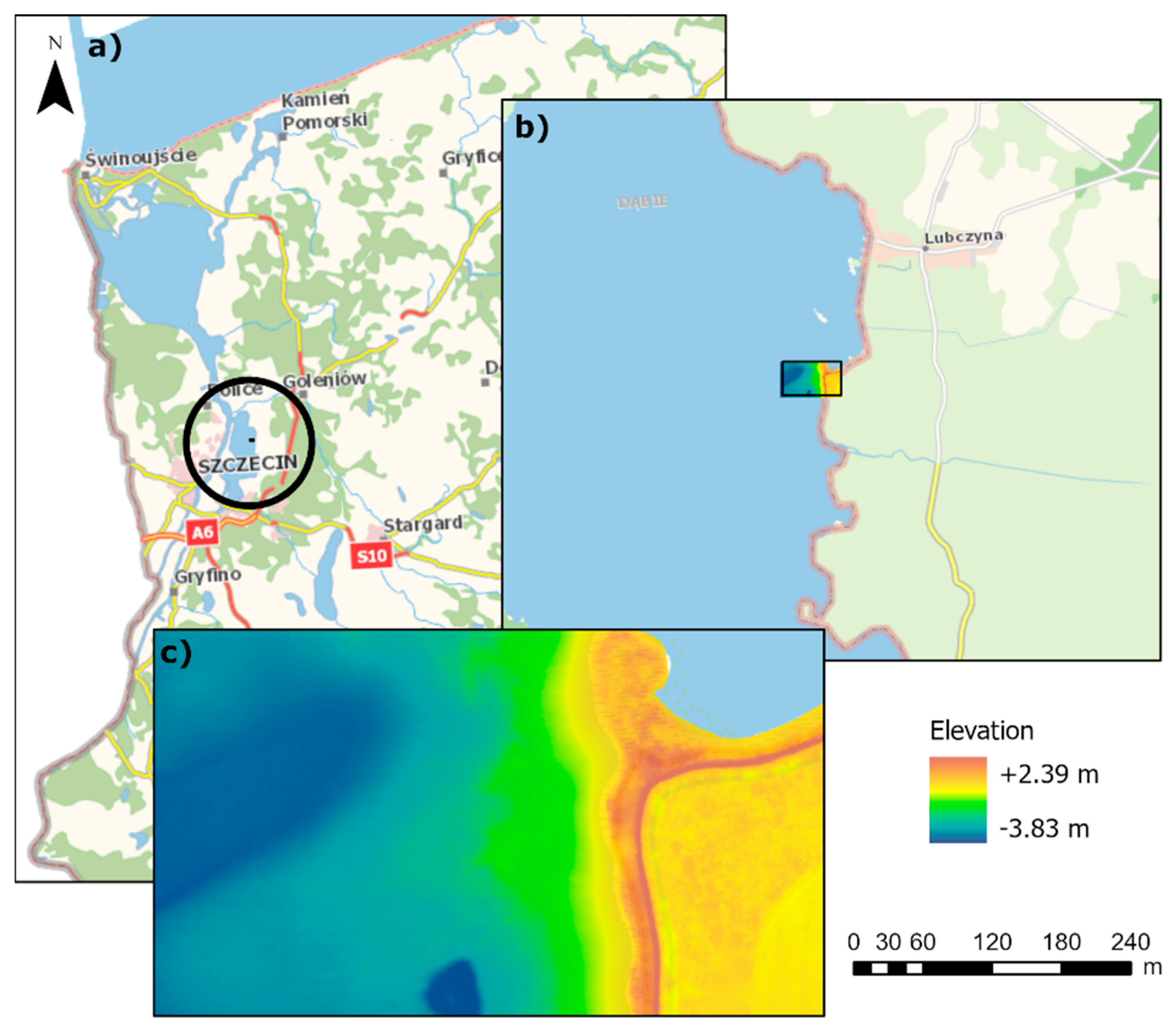
The study area included a section of Lake Dabie, located in Poland’s West Pomeranian Province, along with an adjacent inland area. Lake Dabie is a shallow-water area with an average depth of 2.61 m [
38]. The maximum depth in the study area was 3.82 m. In the direction of the shore, the depths decrease significantly. The bottom is characterized by moderate regularity, and there is one depression and quite considerable shallowing in the strip adjacent to the shoreline. The surrounding land area is characterized by a flat surface. Approximately 5 m from the shoreline, there is a floodbank with a hardened surface covered with mineral aggregate. On the water side, part of the site is overgrown with vegetation characteristic of aquatic areas, dominated by reeds. On the land side, part of the site is overgrown with shrubs (medium vegetation) and grass (meadow area). Single trees are also present. The geographical location of the study area is illustrated in
Figure 1.
Topographic data were collected using the UAS platform. The flight took place on 24 September 2020. The weather conditions were moderately good, partly sunny with wind gusts. The overcast was variable, from partial to total. Before the flight, the photogrammetric reference network was stabilized, and consisted of 6 points distributed evenly over the data processing area. Three points of the photogrammetric matrix were located on the hard surface (on the embankment), two in the area covered with low vegetation, and one on the beach. Control points were also measured to verify the height of the obtained terrain model, and these were used to calculate the errors as an independent set of measurements. The flight was performed at an altitude of 120 m with a DJI Phantom 4 Pro drone using a polarizing filter according to a predesigned flight plan. During the flight, 111 images were acquired, and the size of the compiled area was 0.109 km
2. The last two rows of photos were acquired over a water area. The images from these series were not calibrated (merged with the other images) due to the lack of unambiguous binding points, and therefore, the percentage of calibrated images is 64%. The basic parameters of the equipment used and the data acquired are also summarized in
Table 1.
The low-level data processing of the acquired images was performed in the PIX4D Mapper, a piece of software dedicated to this type of data. The preprocessing of the data was performed to obtain products such as an automatically classified dense point cloud, which was further processed. Georeferencing was performed based on the points measured with the GNSS–RTK (Global Navigation Satellite Systems–Real Time Kinematic) receiver, and the obtained errors are shown in
Table 1. A further processing step was performed in the Global Mapper software, in which a qualitative assessment of the automatic photogrammetric classification of the point cloud was carried out and a manual classification was performed.
In order to obtain bathymetric data, a Hydrograf XXI survey boat was used. This vessel, with a shallow draft, is dedicated to shallow water measurements, especially in inland waters. In the first stage, 79 survey lines were set at a distance of 5 m from one another within the designated survey area. The average depth in the area was 2.74 m.
The survey setup consisted of a Kongsberg EA400 single-beam echo sounder operating at two frequencies, 33 kHz and 200 kHz, with the second frequency used to generate a numerical bottom model from the acquired depths. A Trimble R6 GNSS receiver operating with RTK corrections derived from the VRSNET base station was used as the positioning system. Additionally, in order to eliminate the effects of weather conditions and wave movement, the IMU (Inertial Measurement Unit) SMC-108 motion sensor was used for roll, pitch and heave motion correction. The parameters of the measuring equipment (
Table 2) allowed for a total measurement accuracy within the special category defined by the IHO (International Hydrographic Organization) in specification S-44 [
39]. All data integration and acquisition was performed in the Hypack hydrographic software. Data processing was performed in the SBMAX64 module. First, after the data were imported, navigational data representing the boat’s movements through the survey profiles were analyzed. In the next step, the motion sensor data were subjected to verification. The main focus of the analysis was the depth data. Incorrect readings were eliminated using manual data processing. In most cases where the correct depth reading was uncertain, raw data from digital echograms were used. Before exporting to the ASCII file, the XYZ dataset was corrected via the vertical correction of water level, employing the water level gauge in Szczecin harbor.
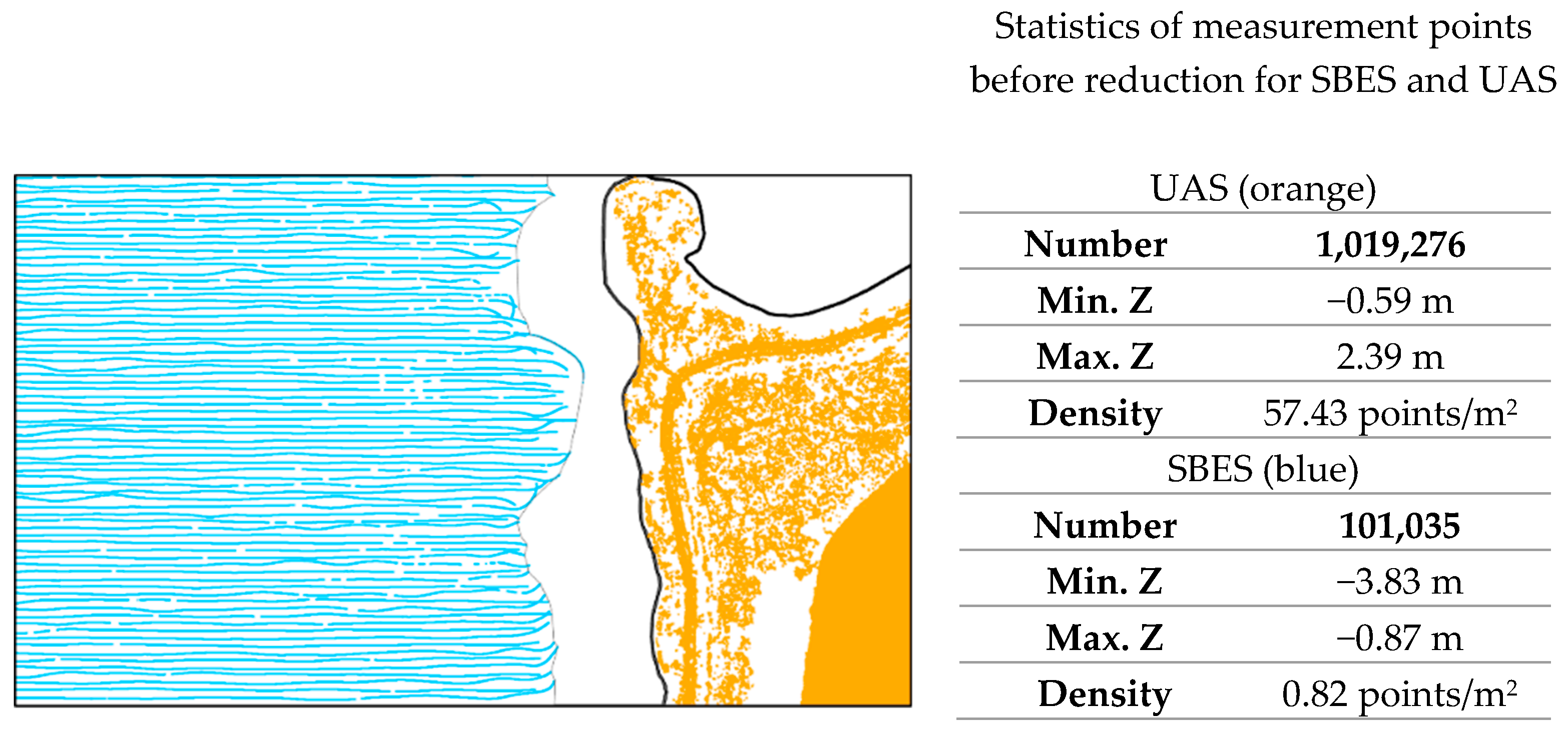
The spatial distribution of the UAS and SBES data after processing and their statistical information are illustrated in
Figure 2. On the left, points obtained with the SBES are shown in blue. On the right, points acquired with the UAS are shown in orange. The final sonar dataset contains 1,019,276 measurement points, and the UAS dataset contains 101,035 points. Negative values of UAS data in the study area have resulted from local depressions (there are water ditches near the dike from the land side).
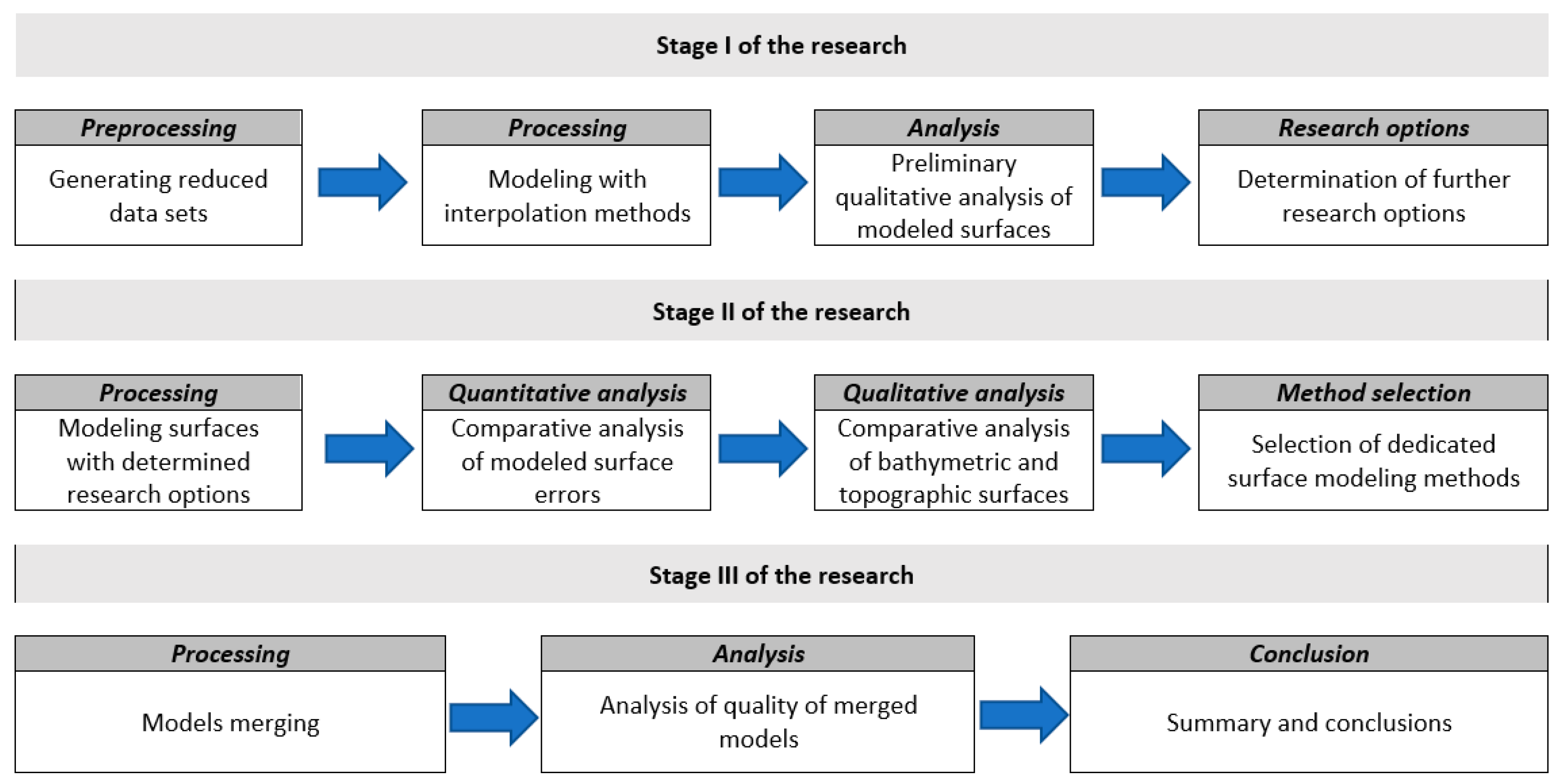
3. Methods
The input data for this study were two sets of measurement data acquired with a single-beam echosounder and using an UAS, as described in
Section 2 (study area and materials). After processing the measurement data, their reduction was carried out, and the result was 39 sets of points with different scales of reduction for data acquired using SBES and UAS separately.
The data in this form were further processed by adding an additional set representing the shoreline to each set of points. This set was created by generating shoreline points at 1 m intervals in the vector data. The purpose of modifying the datasets was to take into account the natural constraint of the modeled surface, which was the shoreline. Modeling was not carried out on combined bathymetric and topographic datasets because, in the shoreline area, point search algorithms can create mixed datasets from which the value at a grid node is calculated. In this case, the height of the topographic area or the depth of the bathymetric area can be calculated from topographic and bathymetric points. This distorts the plasticity of the model, which is different for the bottom and the terrain. The creation of separate models ensures that the shape of the topographic surface is created from the topographic points, while the shape of the bottom surface is created only from the bathymetric points. The shoreline in this case is a natural link between the models.
In the next step, surfaces were created in the GRID structure with 1 m resolution. The authors used the following interpolation methods: triangulation (referred to as TRI), natural neighbor (referred to as NAN), nearest neighbor (referred to as NEN), inverse distance weighted to a power (referred to as IDW), kriging (referred to as KRI), the radial basis function method (referred to as RBF), and minimum curvature (referred to as MIC). In addition, in regard to searching in the interpolation process, two basic methods were investigated: sectorless and four-sector. The sectorless method consists of searching for the measurement points used for interpolation from the nearest neighborhood of a grid node. The selection of points is based on the calculated distance between a measurement point and a grid node. In the case of, for example, interpolation from the 16 nearest measurement points, those with the shortest distances between them are selected. The four-sector method works in a similar way, except that the selection of points takes place separately in each sector. The method used in this study divides the space around a grid node into four sectors. Geometrically, this is achieved by drawing two perpendicular lines intersecting at the grid node. In this way, it is possible to force a search for points in each sector. If, for example, we use a sector search, indicating four points per sector, the search algorithm will search for four points in each sector. In total, we will derive an interpolation from 16 measurement points, but these will be evenly distributed around the interpolated point. In the case of a sectorless search, the distribution of measurement points can vary, which can affect the quality of the modeled surface. In both cases, in order to ensure that the desired number of points is searched, the search radius was set at 150 m. In the first stage of the research, the selection of interpolation variants was made on the basis of the quality analysis. Then, the obtained results were subjected to a visual evaluation of the shape of the modeled surface. This approach made it possible to exclude those options that prevented the correct reconstruction of the surface and to determine the final variants of the study related to the interpolation methods.
In the second stage, the final study options were determined. Qualitative and quantitative analyses were conducted for each modeled surface. For the quantitative analysis, errors were calculated using test points, which constituted an independent set of measurements. Test points were acquired using the GNSS–RTK technology. In the case of the whole water area, a test point was selected from the main bathymetric measurement set, while in the water area with missing data and the land part, measurements were made using a GNSS–RTK geodetic receiver. These points provided the reference measurements for calculating the deviations from the modeled surfaces, from which the absolute values of the mean and maximum errors were calculated. For the bottom models, errors were analyzed for the whole area using SBES data with 19 test points (mean value: −2.70 m; minimum: −3.70 m; maximum: −1.16 m) and for the area with no data using 14 test points (mean value: −0.70 m; minimum: −0.96 m; maximum: −0.40 m). In the UAS data, there were nine test points (mean value: 1.05 m, minimum: −0.27 m, maximum: 2.09 m).
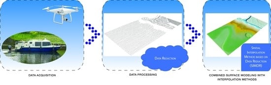
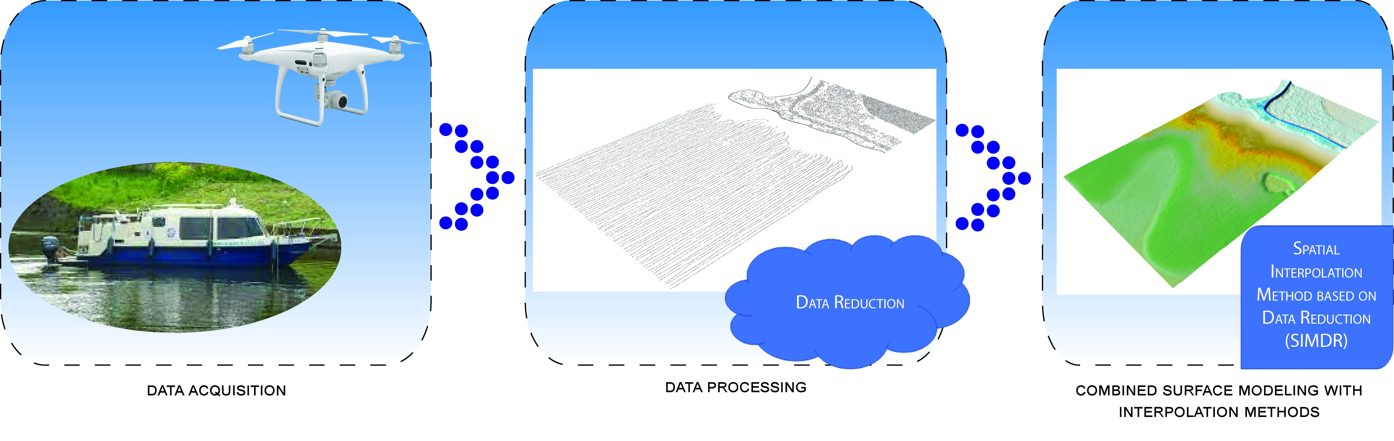
In the third stage of the research, different methods of combining models based on raster data mosaicking techniques—bathymetric and topographic—were analyzed. These analyses provided our final conclusions. The research methodology is presented schematically in
Figure 3.
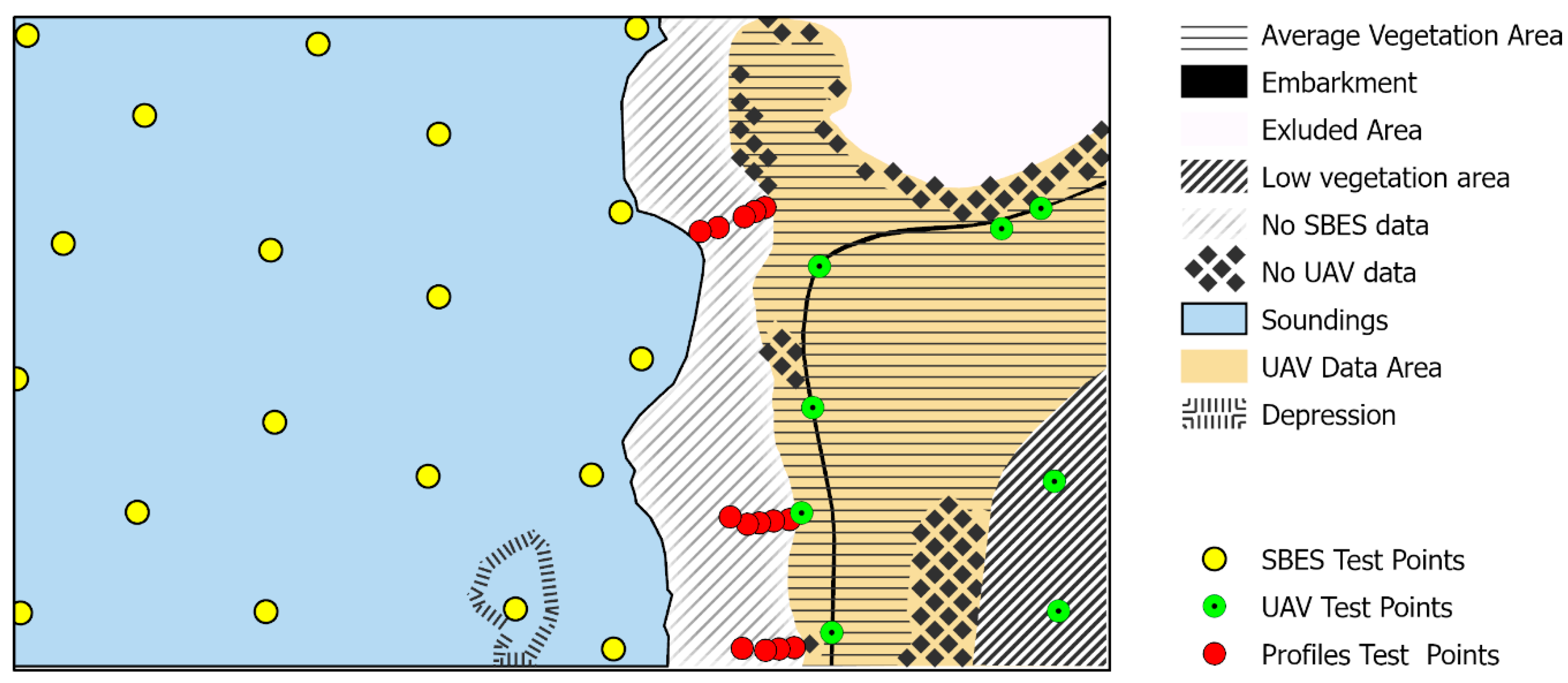
Data with different spatial distributions and point densities were used for this study. Bathymetric data were characterized by a regular spatial distribution, which resulted from the methods we used for their acquisition from the planned survey profiles. The UAS datasets were generated from aerial photographs as a point cloud. A characteristic of the data used is their dispersed spatial distribution, which makes the surface interpolation process more difficult [
17]. In addition, smaller areas with missing points belonging to land cover (high and medium levels vegetation) were created through data processing after filtering out points belonging to land cover. The lack of ground data in areas of dense vegetation is related to the specifics of obtaining these data; a dense point cloud is created on the basis of photographs, so there is no possibility of obtaining height information about parts of the ground that are not visible on the images (under dense vegetation, buildings). Data were also lacking in a narrow strip near the shoreline. An important area in the interpolation process was the shallow-water area. These shallow depths made it impossible to take measurements with a hydrographic vessel; as such, here, the data had to be interpolated based on extreme measurement points, which comprised shoreline points and bathymetric data. In addition, the surface characteristic elements were analyzed. For the bathymetric model, these were the slope of the bottom surface and the depression, and for the topographic model, these were the floodwall and the areas of medium and low vegetation. All the mentioned datasets and surface elements are presented in
Figure 4.
The datasets used during the study were reduced using the Reduce Point Density method, which is implemented in ArcGIS software. This reduces the number of points in the sets depending on the Nominal Start Thinning Radius (R) parameter and the method of selecting individual points. The first parameter specifies the radius of the circle within which a particular point will be selected. The remaining points are reduced. The second parameter is the selection method. Two variants were used in this research: MAX and MIN. In the first, the reduction is based on retaining the data with maximum values (MAX variant), while in the second, the minimum values are retained (MIN variant). Geodata in the form of points can be transformed via the following algorithms [
40]:
Aggregation—combining more points into one;
Simplification—removing objects in order to properly present those remaining;
Typography—retaining the predominant source symbolization of point objects while removing points;
Regionalization—drawing a boundary around a group of point objects and creating a new surface object from it;
Selective omission—selecting objects that are more significant while omitting objects of lesser significance.
The used method can be classified as selective omission. In this case, points in a certain area (circle) with the smallest or largest Z values were selected. The data were reduced over a range of R parameter values, from 0.2 m to 4 m, with an interval of 0.1 m. This gave a total of 39 sets of points, with different scales of reduction for data acquired using SBES and UAS for the two variants MIN and MAX. In total, 156 reduced datasets were obtained for further analysis.
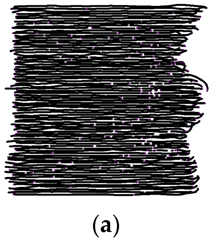
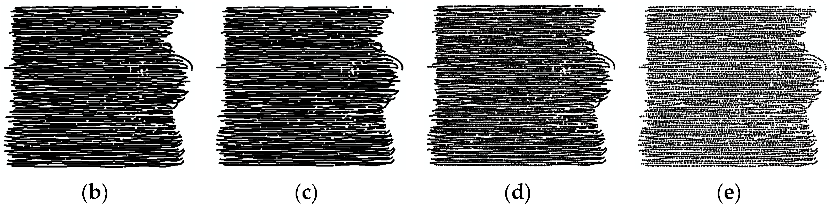
Figure 5 shows an example of reduction for data acquired using SBES.
The figure above shows the spatial distribution of the input data and the reduced sets with radius values (0.2 m, 1 m, 2 m, and 4 m) specifically selected for retaining the minimum values. The initial set contains 101,035 points, with a minimum depth of −3.83 m, a maximum depth of −0.87 m, and an average depth of −2.79 m. The reduction results for the SBES data with the main characteristics are shown in
Table 3.
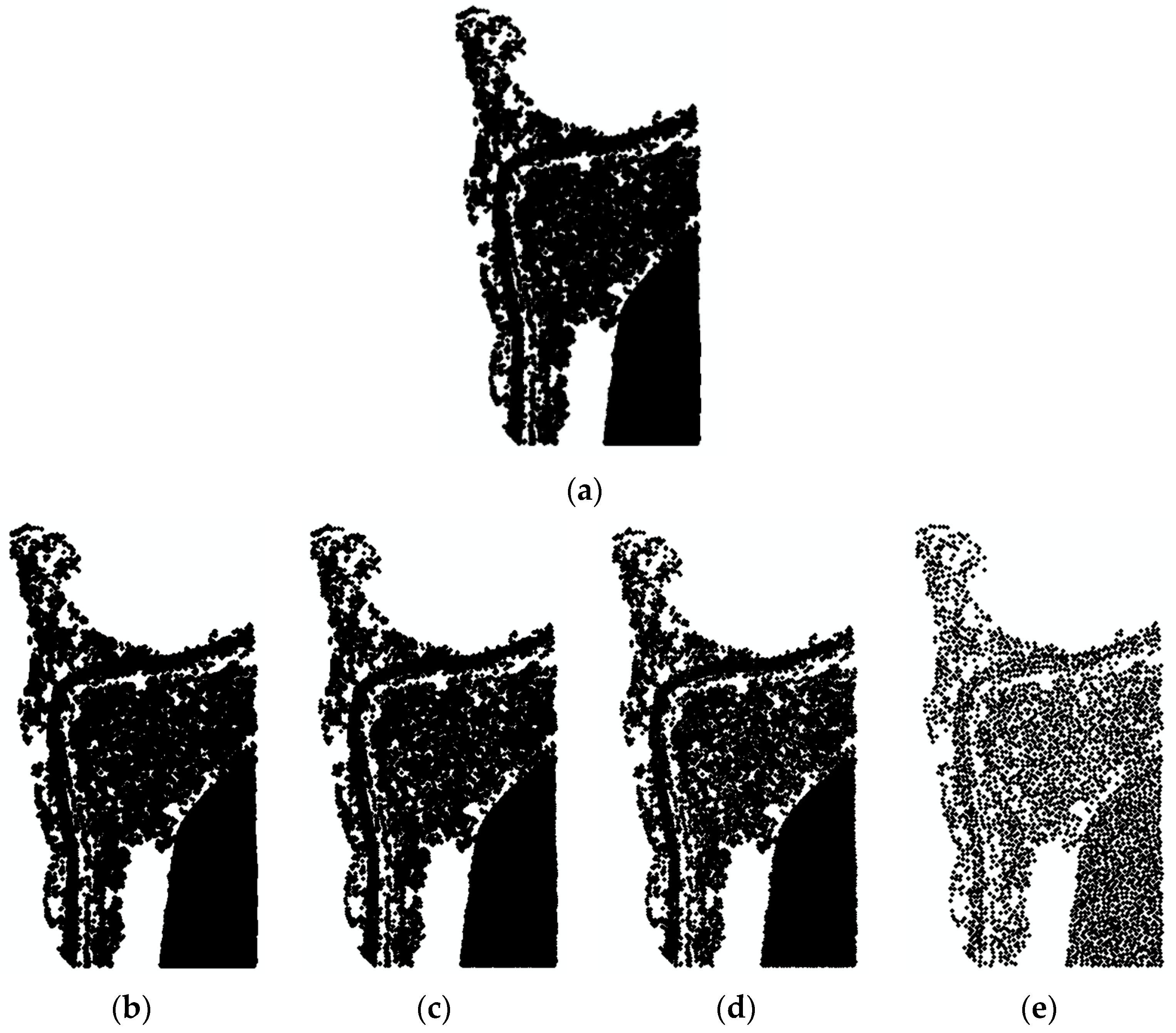
Figure 6 shows an example of reduced data acquired with the UAS system. The example uses the same parameters as
Figure 5.
The initial set contains 1,019,276 points, wherein the minimum height is −0.59 m, the maximum height is 2.39 m, and the average height is 0.32 m. The reduction results for the UAS data along with their characteristics are shown in
Table 4.
A total of 156 reduced datasets were obtained for further analysis. Different surface interpolation methods were selected for the study. These included parameter-free, parameter setting, local, and global surface interpolation methods. For methods interpolating the surface locally, the effect of the search method was also investigated. Automated interpolation was performed using the Surfer 20 software with a scripting language. The methods, along with a brief description and the parameters chosen here, are summarized in
Table 5.
4. Research
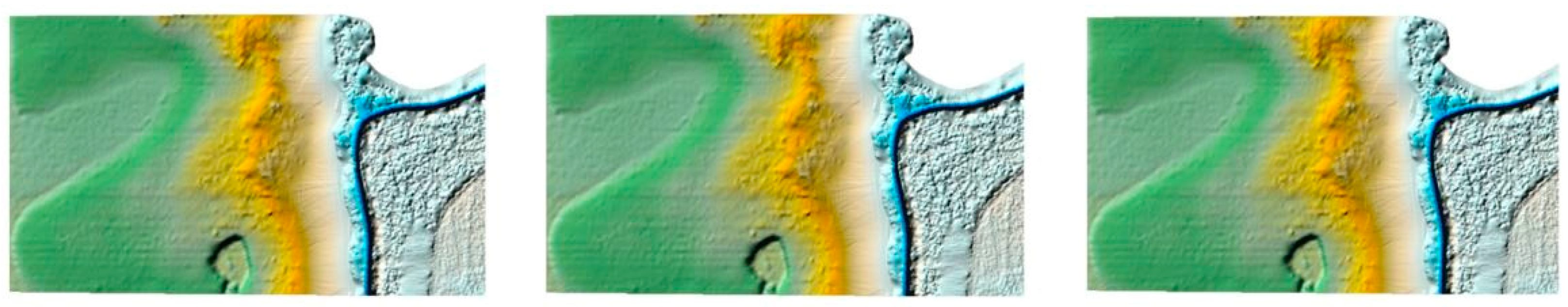
In the first stage of the research, all modeled surfaces were analyzed. Preliminary qualitative analysis, consisting of the assessment of the correctness of the modeled surface, allowed us to reject some of the options. In this respect, the locally interpolating methods (IDW, kriging, RBF) without data search sectors were found to have low usefulness. The reason for this is the poor surface representation in areas with few data, which manifested in the form of artifacts. A comparison of models used in the area without bathymetric data is shown in
Figure 7. A color-coded depth scale is used for each height within the model. As can be seen, in the center of the area without bathymetric data, the surface is characterized by a clear lack of continuity. The next step was to determine the number of points used in the local interpolation. In this respect, the plasticity of the terrain representation was used as a criterion of correctness. While the number of points was found to have less influence on the surface reconstruction in the area with data, the number of points was important in areas with no data. Based on a visual assessment, 12 points per sector was selected as the correct number of points, resulting in an interpolation of 48 survey points in total. Following visual comparative analysis, it is also possible to estimate the qualitative differences in surface modeling using sectorless and sector search points. In the case of sector searching, the surface in the no-data area is characterized by continuity, i.e., there are no artifacts representing sudden depth changes.
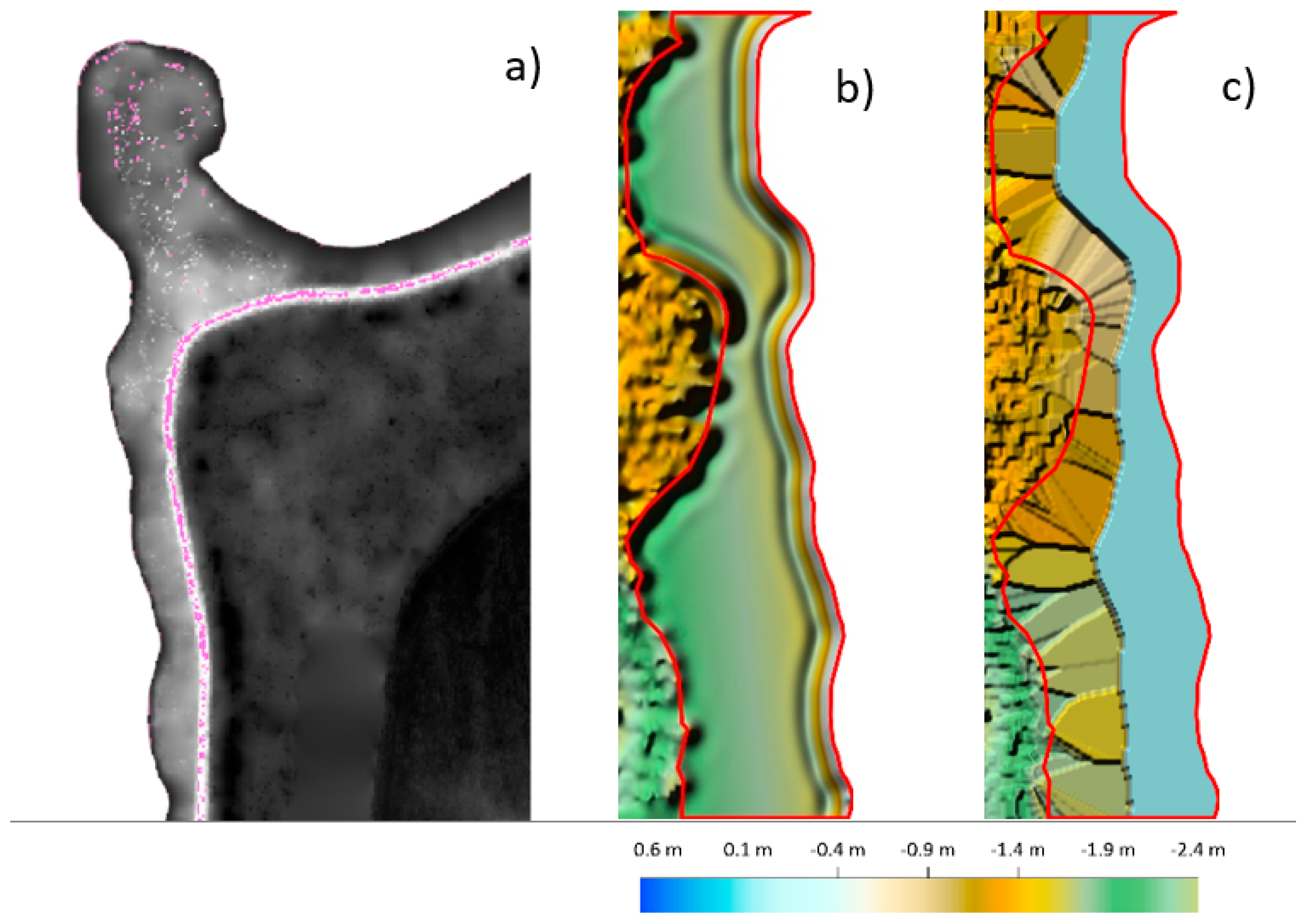
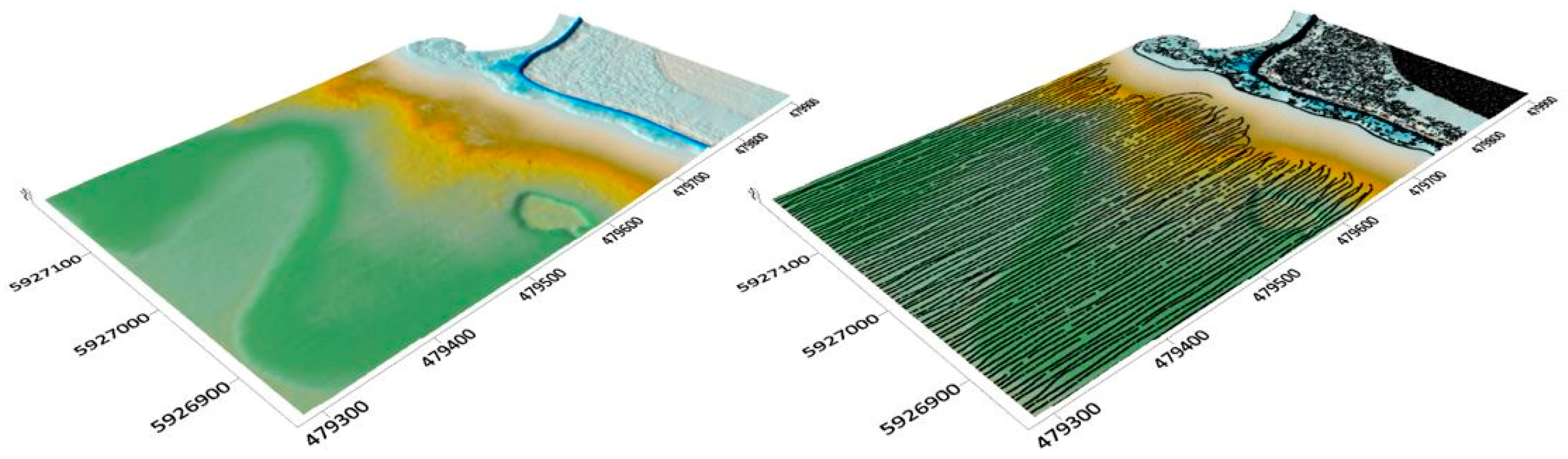
In interesting cases, problems with complete surface modeling via the natural neighborhood method were noted. For the UAS data with a very small degree of data reduction (level 0.2–1.0), pixels were found in the surface with missing data (
Figure 8). In this case, we also used a color-coded depth scale for each height in the model. The lack of data was particularly evident on the flood embankment as well as in the upper part of the area. Therefore, this method was not considered further in the study. Other methods that were not qualified for further study were the minimum curvature method and the nearest neighbor method. These methods generated artifacts in the area with no SBES data (
Figure 8).
In summary, after the first stage of research, the analysis of interpolation options using sectorless point search and natural neighborhood, nearest neighbor and minimum curvature methods was abandoned. The triangulation, kriging, RBF, and IDW methods were qualified for the next stage of research. Of the rejected methods, natural neighborhood can also be considered, as no deficiencies were seen in this method’s modeled surface, and it showed a higher degree of data reduction. However, this requires additional qualitative analyses of the modeled surface in terms of the data gaps present.
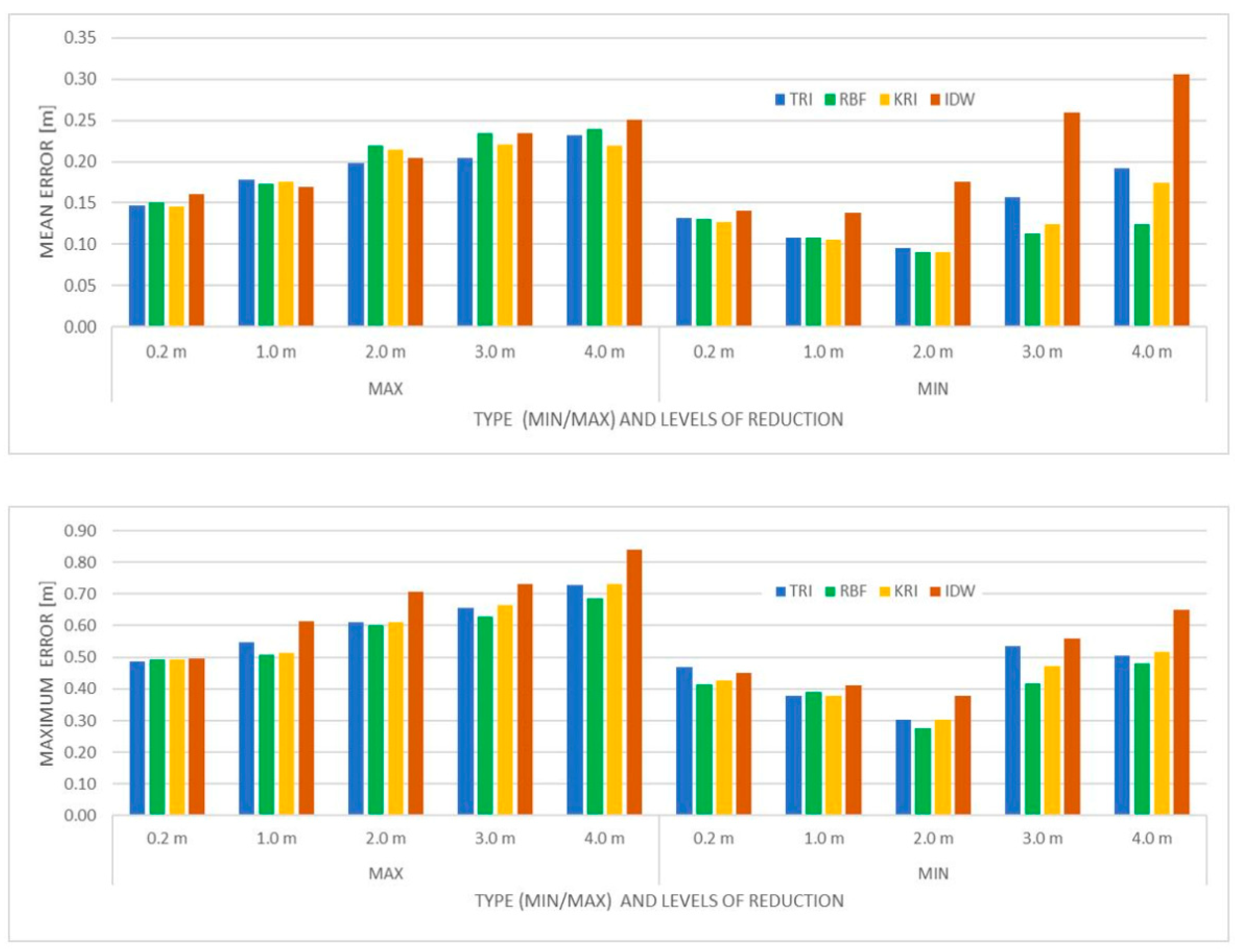
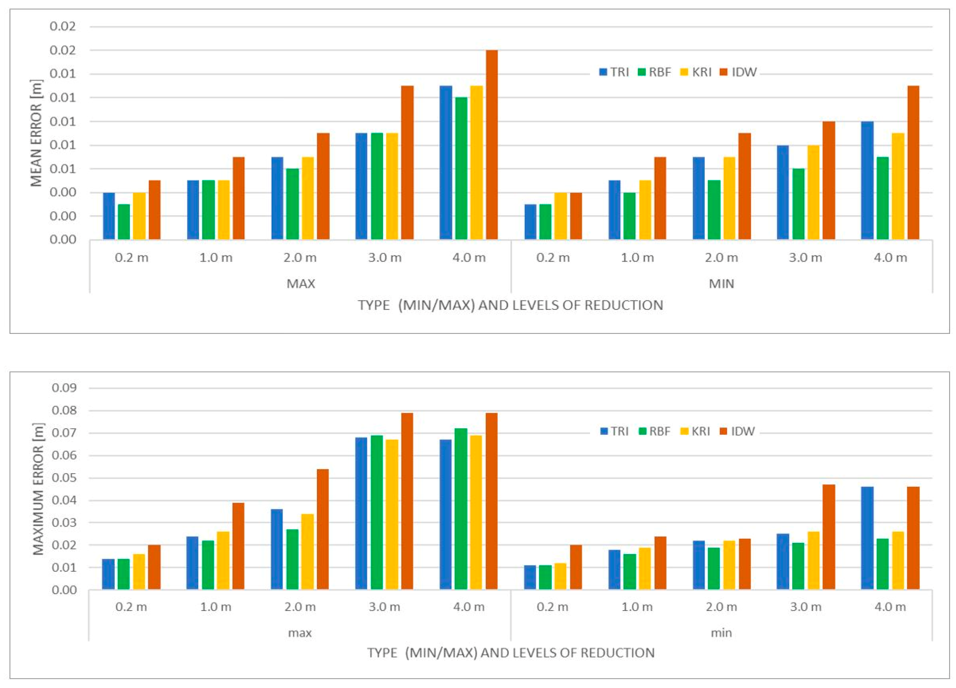
The second stage of the research involved quantitative and qualitative analysis. The quantitative analysis was based on a comparison of mean and maximum errors related to the four methods. Basing on the graphs for all the samples, in the final stage, the quantitative results of four levels of data reduction—0.2, 1, 2, 3, and 4—were compiled. The choice of these levels was preceded by the analysis of errors via graphs constructed for all the samples, which allowed us to select representative results reflecting the characteristic relations between method and level of data reduction. The errors are summarized in
Figure 9,
Figure 10 and
Figure 11.
Analyzing the SBES data, it can be concluded that the errors increase with data reduction for both MIN and MAX methods. The errors have smaller values under the MIN reduction method. The mean and maximum errors both differ depending on the interpolation method. The highest values are derived from the inverse distance method, followed by triangulation, kriging, and the RBF method. It should be mentioned here that the errors for each variant differ within the range of about 1 cm, which may be a negligible value when choosing a method. Greater differences become apparent in the case of the maximum errors, which take much smaller values under the MIN reduction method. The mean values for all trials are 47% smaller (2 cm). Under the MIN method, on the other hand, the mean errors are 17% (0.01 cm) smaller, which in principle could also be a negligible value. Another observation is that, under the MIN method, the maximum errors derived by the kriging and RBF methods change slightly from 1 cm to 3 cm as the level of data reduction increases. According to the quantitative criterion, the RBF and kriging methods perform best.
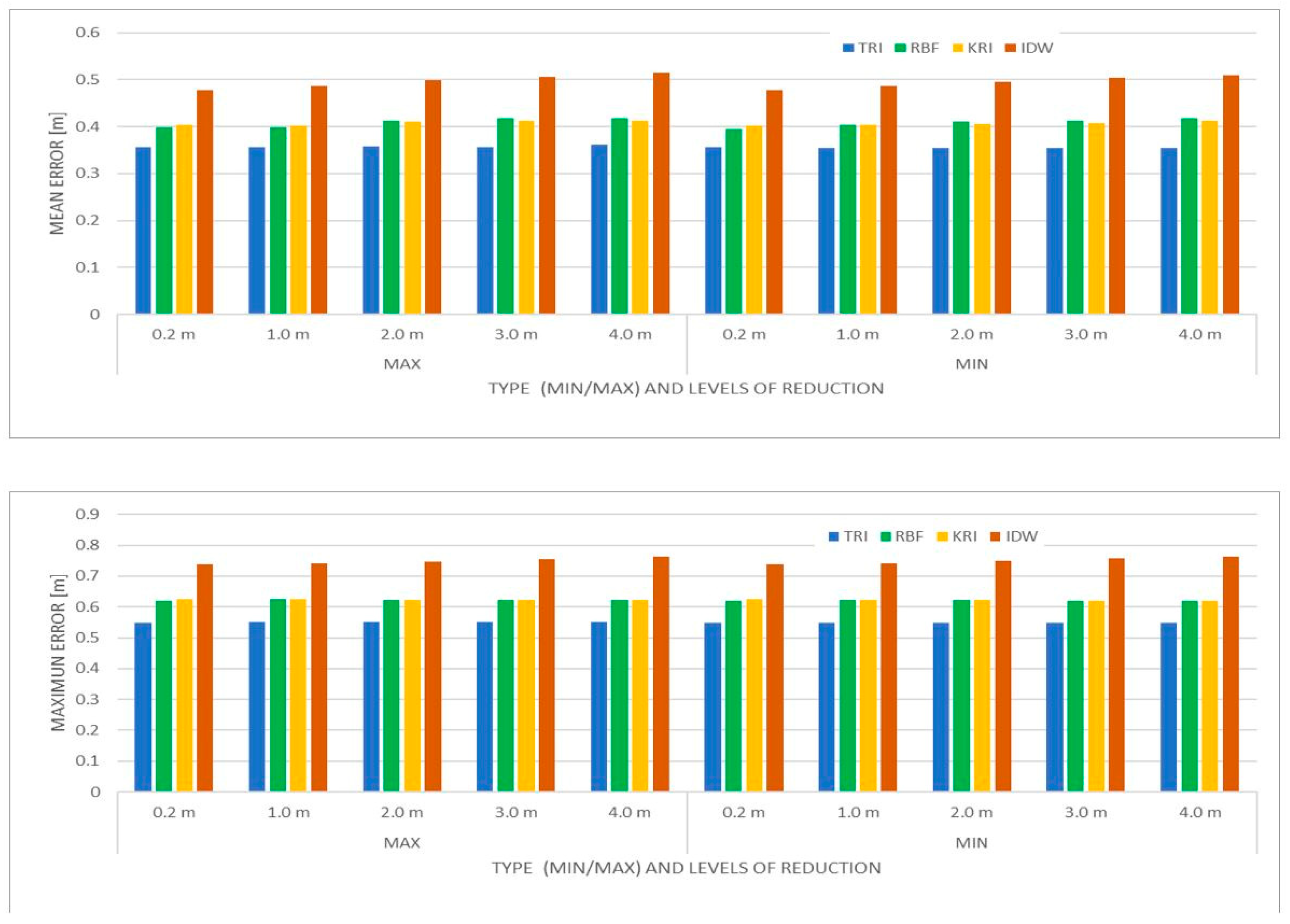
For UAS data, a linear increase in the mean and maximum error values can be observed under the MAX reduction method. The relationship is slightly different for data reduction via the MIN method. In this case, a decrease in error values up to a reduction rate of 2 can be observed, followed by an increase. This applies to the values of both mean and maximum errors. Comparing the errors for the MAX and MIN methods, a similar relationship can be observed as in the SBES data—the errors are smaller under the MIN reduction method. In regard to the MAX reduction method, the best results can be achieved using the triangulation and kriging methods, while for the MIN reduction method, the RBF and kriging methods are best. By far the worst results are obtained with the inverse distance method, especially for the MIN method. Smaller errors can be obtained with the MIN reduction method, with the average errors reduced by 27% (6 cm) and maximum errors reduced by 29% (22 cm).
For the area of the water body with no data, the results for all levels of reduction are similar, meaning its influence is practically negligible. It can also be seen that the average errors for all samples are much larger than for the area with data, at 42 cm. In contrast, for the SBES data in the area with data, this value is 1 cm, while for the UAS data, it is 17 cm. It can be concluded that the best results can be achieved using the triangulation method, followed by kriging and RBF (comparable results) and then the inverse distance method.
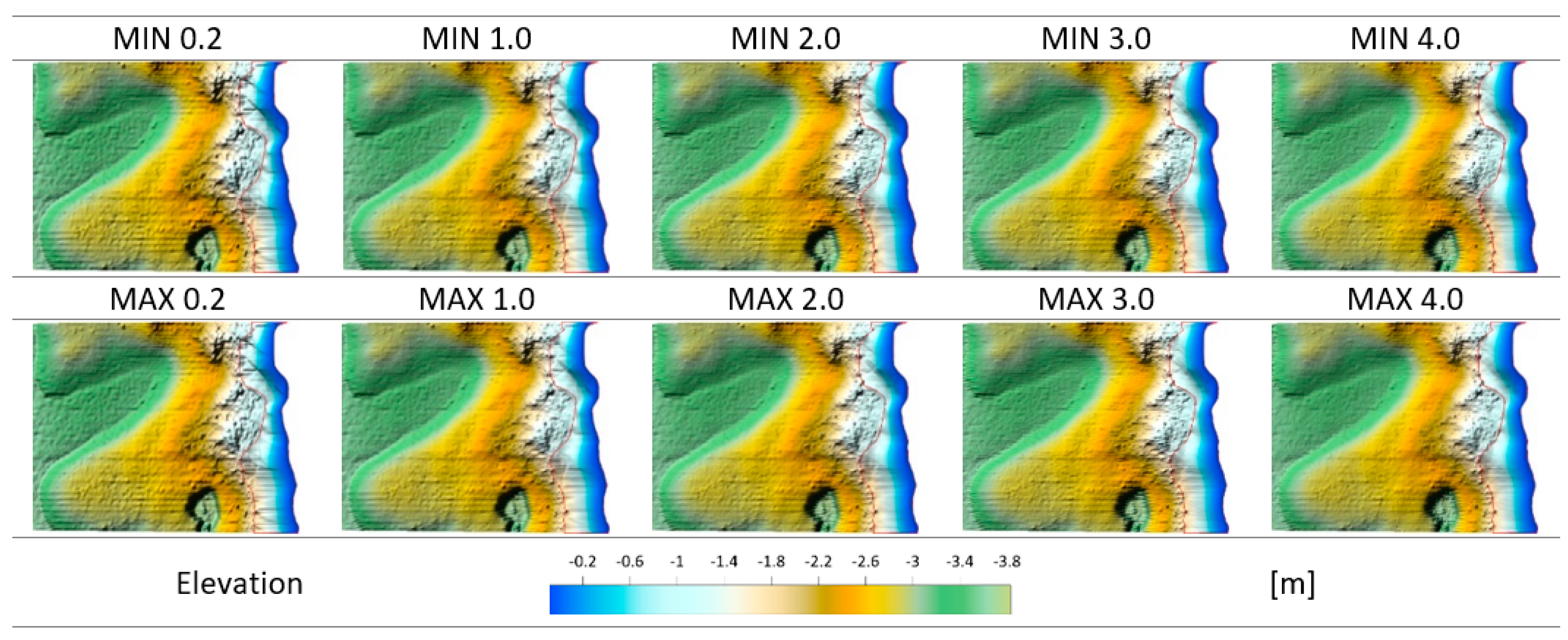
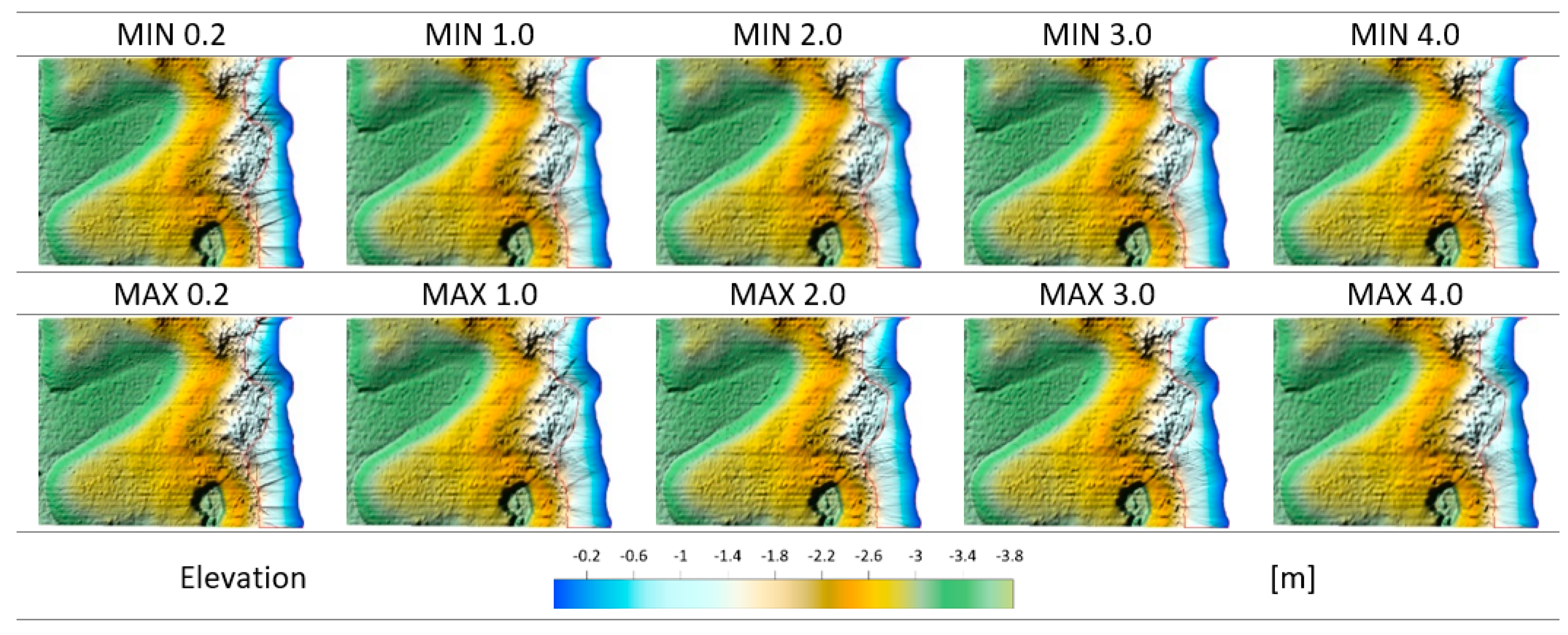
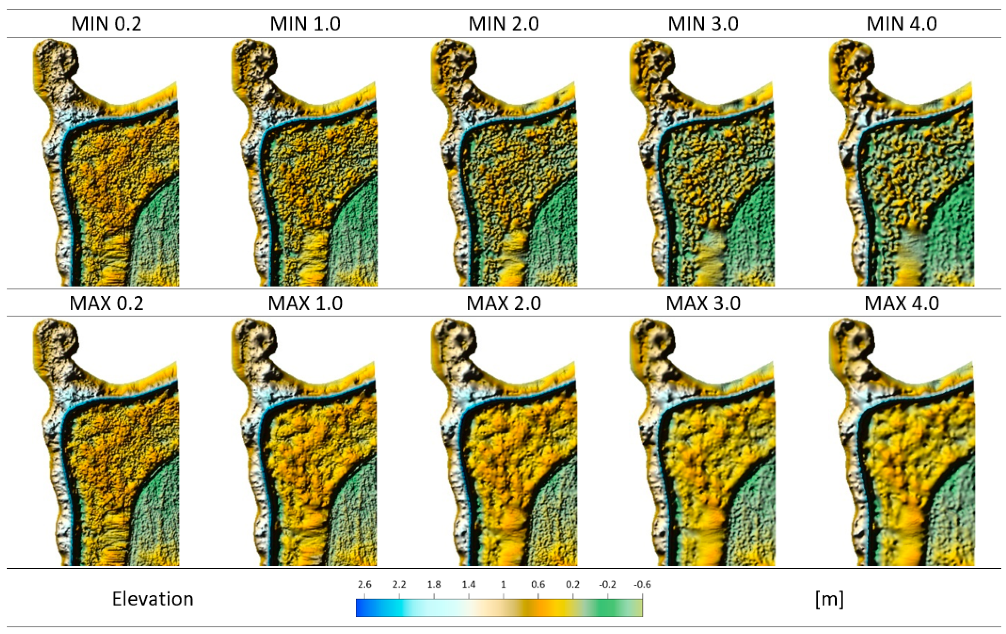
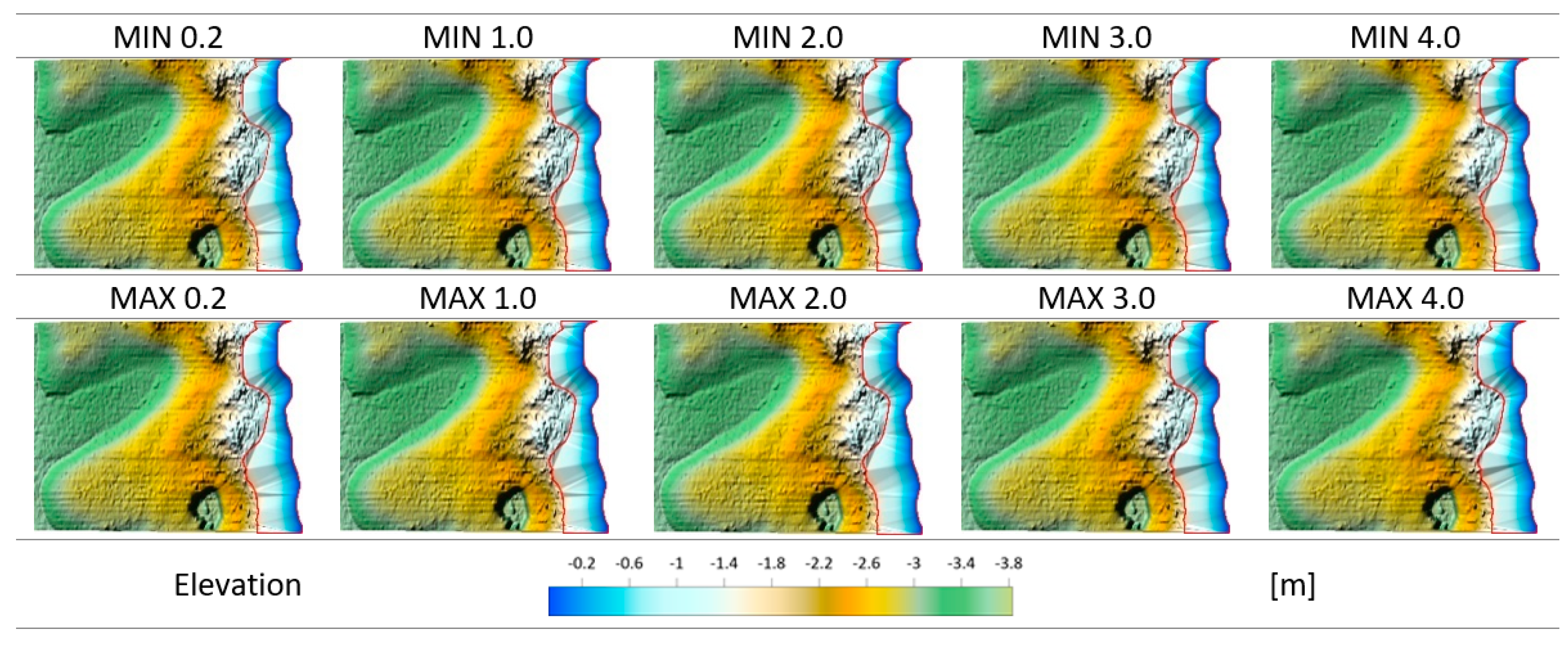
The next step during the research was a qualitative analysis of the previously selected models. The modeled surfaces are shown in
Figure 12,
Figure 13,
Figure 14,
Figure 15,
Figure 16,
Figure 17,
Figure 18 and
Figure 19. DBM is the Digital Bottom Model, DTM is the Digital Terrain Model, MIN and MAX denote the data reduction methods, the numbers next to MIN and MAX denote parameter of reduction (R), and a colored depth scale is applied to the surface models.
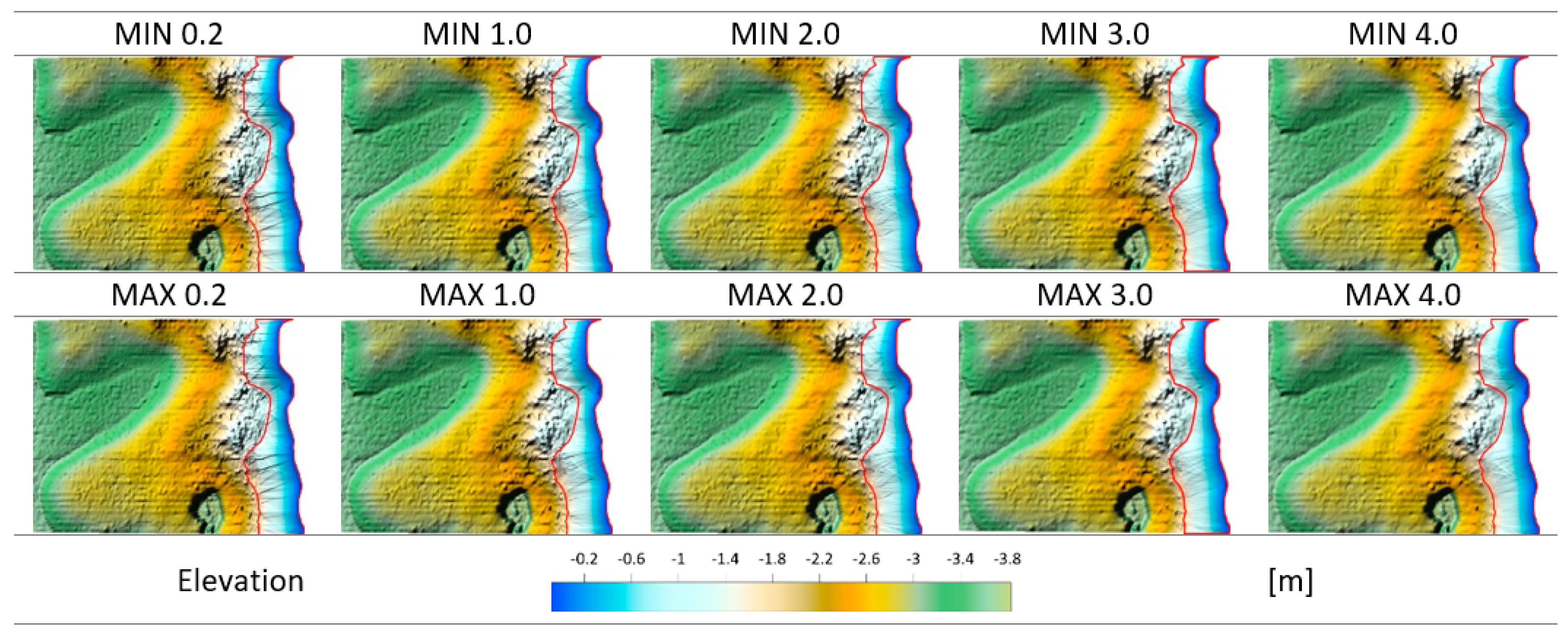
Figure 12 shows the surfaces created from the SBES data using the triangulation method. Each of the created models presents a smooth surface with correct terrain plasticity. However, some of the areas exhibit profile lines related to the source data, which make the perception and interpretation of the created models easier. The terrain slopes are modeled correctly. In the area lacking data, a surface was created based on elevation values derived from polygon vertices. Due to the lack of available data in this area, the correctness of the created surface cannot be assessed, but the visual appearance of the model is acceptable. The impact of reduction for this model and this type of data is negligible.
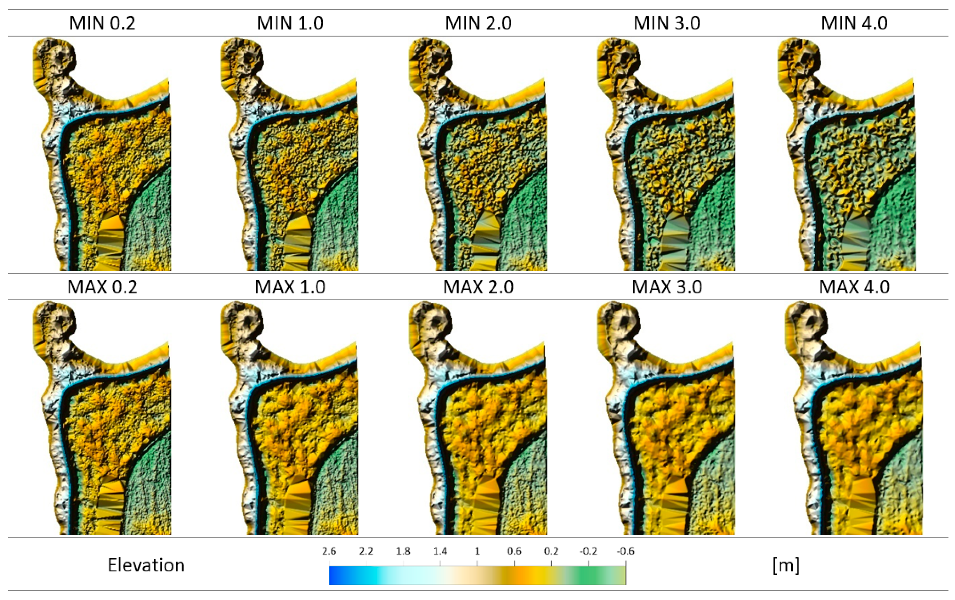
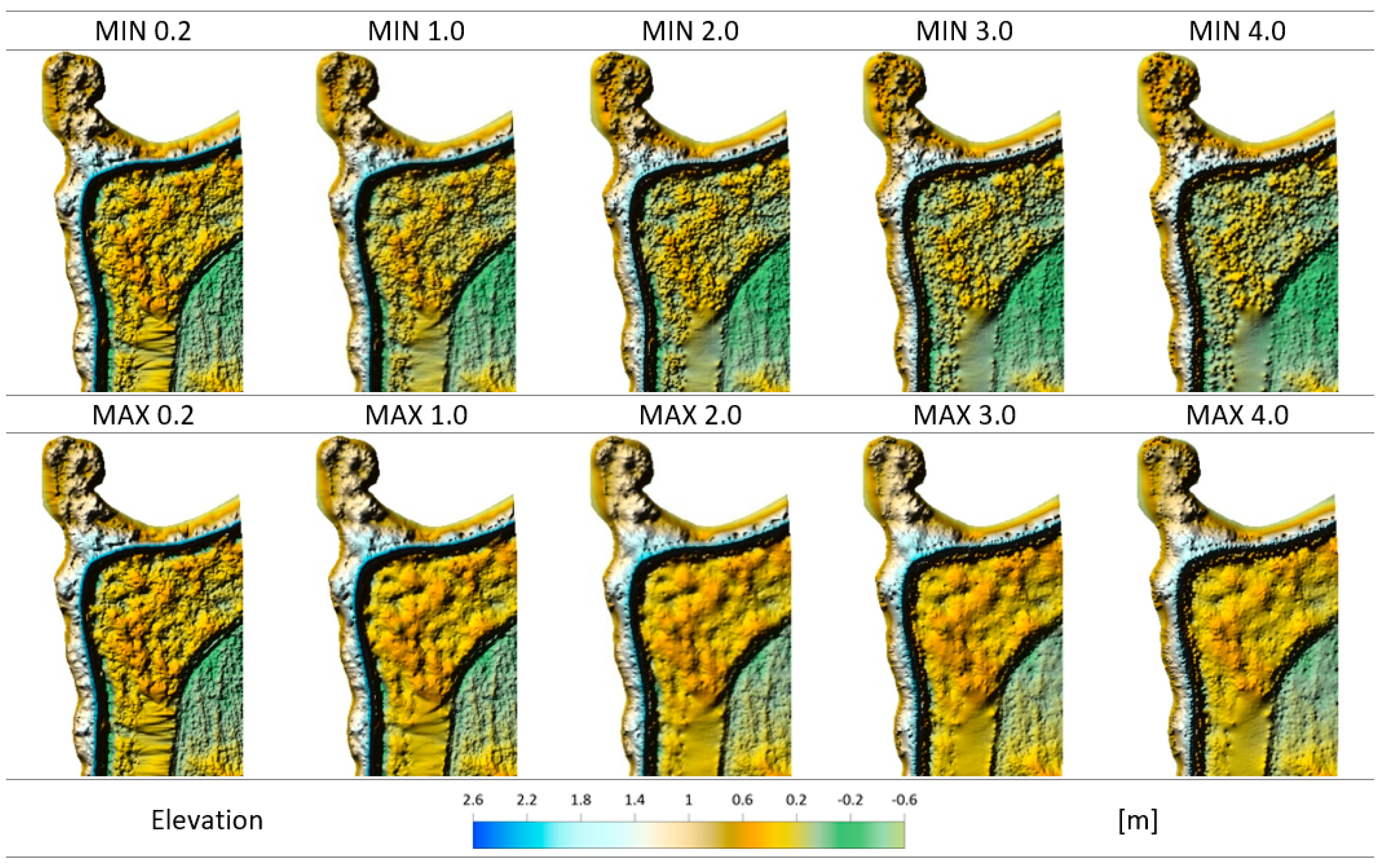
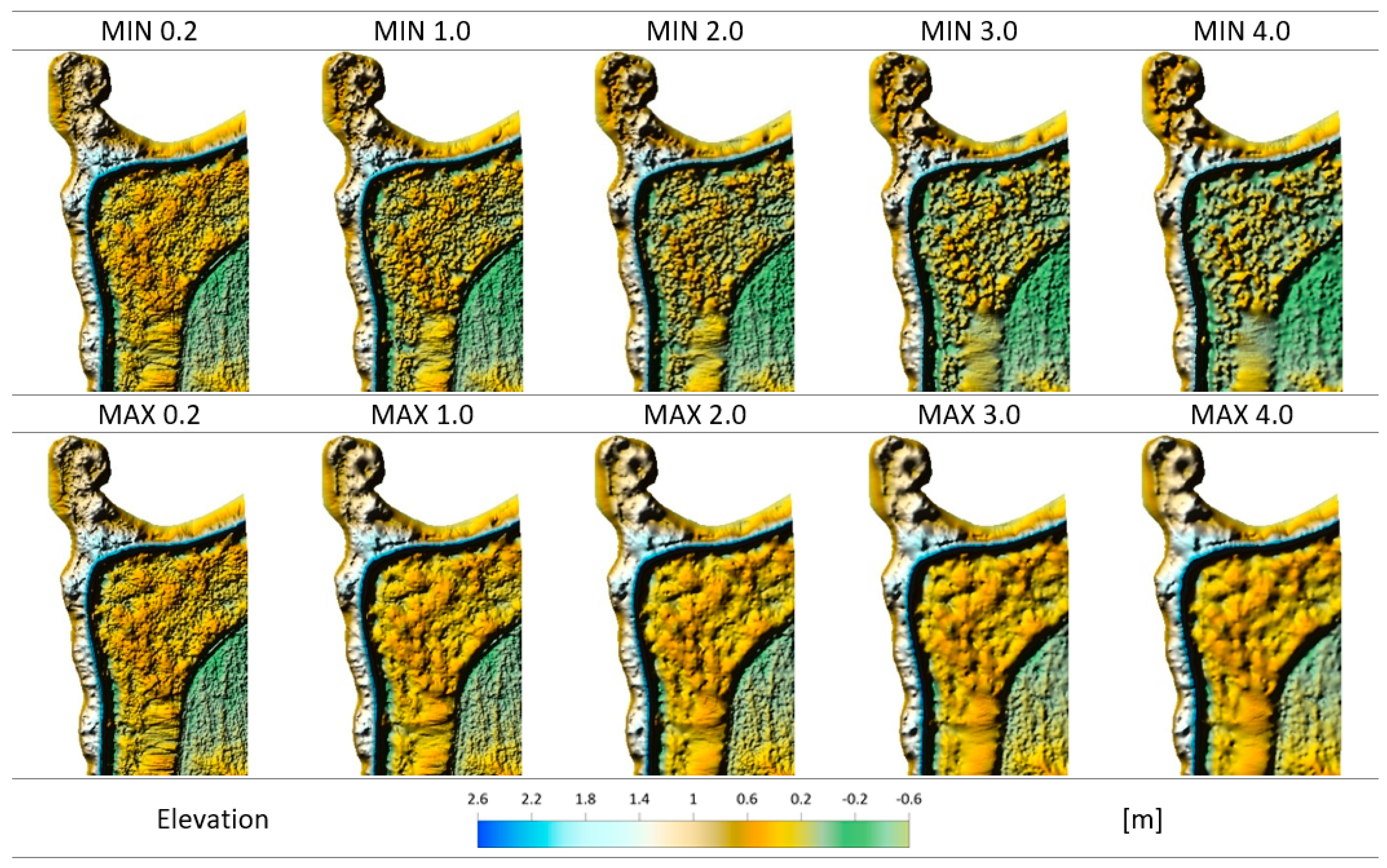
Figure 13 shows surfaces created from photogrammetric data derived from UAS using the triangulation method. First, it is worth noticing that both the type of reduction (MIN, MAX) and its level (0.2, 1.0, 2.0, 4.0) have a significant impact on the final surface obtained. The level of reduction has a significant impact on the visual perception and generalizability of the final model. The type of reduction has an influence on elevation modeling, especially in the area with vegetation cover (low and medium). Models obtained with the MIN method are rougher. It is also important to note the modeling of the embankment, which becomes increasingly fractured as the input data decreases. Areas of high vegetation, i.e., small number of ground points, were modeled slightly differently on each of the analyzed models, with the most correct modeling offered by the MAX 4.0 method. All models obtained with this method are plastic and interpretable; the models lack artifacts and other deformations.
Figure 14 shows the surfaces created from the SBES data using the inverse distance method. Qualitative analysis was performed on models with four-sector interpolation using 12 points per sector. The overall plasticity of the terrain is correct but becomes worse as the level of reduction increases; at the highest reduction, and especially at points of depression, small artifacts (short horizontal lines) are visible, making interpretation difficult. The representation of the area with missing data varies with the level of reduction. The higher the degree, the smoother the area of missing data. Under the MIN method, the nearshore area (near the line of missing data) is rougher.
Figure 15 shows the surfaces created from the UAS-derived data using the IDW method. A qualitative analysis was performed on models with four-sector interpolation using 12 points per sector. The effect of the level of data reduction on the results obtained is significant. High reduction eliminates characteristic terrain forms. The MIN method with a reduction level of 4.0 causes significant terrain deformations, which make correct interpretation of the surface impossible. The results obtained with the MAX method for the same degree of reduction are significantly better, although the representation of the dike is also incorrect in this case. For small levels of reduction, the terrain plasticity values are correct—smoother for the MAX method, rougher for the MIN method.
Figure 16 shows the surfaces created from the SBES data using kriging methods. The qualitative analysis was performed on models with four-sector interpolation, 12 points per sector. The MIN and MAX methods produce very similar results when modeling surfaces from the profile data. The modeling is also very similar when performed on data with different levels of reduction. The obtained models are plastic and allow for good interpretation.
Figure 17 shows surfaces created from the UAS data using the kriging method. Qualitative analysis was performed on models with four-sector interpolation, 12 points per sector. The main difference between the MIN and MAX methods is the occurrence of greater terrain roughness in coastal areas and average vegetation in the MIN method; the MAX method produces a smoother surface. There is a considerable loss of terrain detail at a high reduction level, which is most visible in the embankment area. The overall plasticity of the modeling is correct.
Figure 18 shows the surfaces created from SBES-derived data using the RBF method. There is little difference between the MIN and MAX reduction methods; the most noticeable differences appear at the high reduction level (4) in the area bordering the missing data area; there is greater roughness under the MAX method. At a lower level of reduction, the changes between MIN and MAX are unnoticeable. The lack of reduction has the greatest effect on the modeling of the area with missing data and the boundary area. The plasticity of the area is correct.
Figure 19 shows the surfaces created from the UAS data using the RBF method. The qualitative analysis was performed on models with four-sector interpolation with 12 points per sector. This method provides very similar results to the kriging method for this dataset. The main difference between the MIN and MAX methods is the presence of greater terrain roughness in the coastal areas and medium levels of vegetation in the MIN method; the MAX method also provides a smoother surface. The plasticity of the modeling is correct; there is a loss of details with the increase in data reduction. The area lacking data is modeled correctly—a smoother surface is obtained with a higher level of data reduction.
The qualitative analysis considering the topographic surface elements is summarized in
Appendix A (Qualitative analysis for surfaces created from SBES data) and B (Qualitative analysis for surfaces created from UAV data). Based on the qualitative analysis, it can be concluded that the modeling of SBES data is achieved comparably well between the triangulation, kriging, and RBF methods. Only the models obtained via the IDW method give slightly worse results, which is reflected in the formation of artifacts at the higher levels of data reduction on the higher parts of the bottom’s slope. In the case of triangulation, a tendency toward the slight mapping of profiles was noted, perhaps related to the interpolation technique’s preserving of the source survey points in the structure. Similar conclusions can be drawn from the UAS data. All the methods—triangulation, kriging, RBF, and IDW with sector searching—provided visually correct surfaces. However, it should be noted that the IDW method again performed the worst with the given level of reduction (above the second degree can result in a significant loss of detail in terrain microforms). The triangulation method, on the other hand, performed less well in terms of creating a uniform surface in the area lacking UAS data. The MIN reduction type produced a rougher surface. Based on the qualitative analysis, it can be concluded that the methods produce comparable qualitative surfaces, but artifacts can be identified, as is well demonstrated by the IDW method. This method tends to produce artifacts and lose significant detail at higher levels of data reduction. In conclusion, visual analysis should be supported by results obtained from quantitative analysis, and the choice of the appropriate method should be made accordingly.
Combining Models
Models were developed separately for bathymetric and topographic data, and, therefore, did not overlap. The option of combining models in overlapping areas was omitted in this case; therefore, the effectiveness of three resampling methods was evaluated: nearest neighbor, bilinear interpolation, and cubic convolution. Here, the merging line was not recognizable, which qualifies all the methods for resampling this type of raster. Interpolation within the boundaries of the area is important in this case, and this was achieved by inputting the corresponding shapefile. In this case, the area outside the polygon had the status of “No Data”. A 2D illustration of the combination of models using the kriging method (four-sector search, 12 points per sector, minimum reduction method at the 2 m level) is given in
Figure 20, and a 3D view is given in
Figure 21.
5. Discussion
The aim of the study was to develop a combined bathymetric and topographic model. As can be seen, the choice of interpolation method and the degree of data reduction are not straightforward. As far as interpolation methods are concerned, various studies can be found identifying the best. However, it is important to realize that each data type has a different density and may have a different spatial distribution, and so a different method may be required in each case. The research conducted in this paper exemplifies this. For the SBES data, the differences in the errors obtained are so insignificant that practically any method can be used. In the case of UAS data, the best results can be obtained using the RBF and kriging methods, while in the case of a body of water without bathymetric data, the triangulation method is favored. Quite clearly, the IDW method can be abandoned, as it gives larger errors and is more prone to artifacts and significant losses of detail with greater degrees of data reduction. Based on these observations, the question can be raised as to whether there is really a universal method. Certainly, the choice of such a method will entail some compromises. Therefore, a qualitative analysis was performed to evaluate the methods, seeking to determine the best method via the correctness of the plasticity of the reconstructed surface. An incorrectly created surface can lead to misleading conclusions or the qualification of artifacts created by the method as surface microforms. Given the final results, the authors decided not to choose a universal interpolation method, and they selected a method on the basis of the results of the modeling process. This is particularly relevant given the results derived using the MIN reduction method for UAS data. In this case, as the reduction increased, the errors started to decrease up to the 2 m reduction level and then started to increase. Would such a relationship occur in a similar but different dataset? It is difficult to answer this question, and so it is reasonable to employ automated data processing and the automated selection of an appropriate method and degree of data reduction. Such a process can be implemented using scripting programming languages. As can be seen in the results of the study, such a process should be carried out separately for bathymetric and topographic data, due to the different levels of reduction that can minimize the errors obtained by specific interpolation methods.
The proposed method was developed for data obtained from a small area, which typically resulted from the operational limitations of the measuring vehicles used. However, taking into account the similar structure of data obtained by modern remote sensors, such as topobathymetric LIDAR, i.e., high-density sets with a regular or scattered spatial distribution, it is possible to use the method for other types of areas, including those with a larger size. The proposed calculation algorithm includes a qualitative and quantitative assessment module; hence, when testing the method on other areas with different topographic features, it is possible to determine whether the method can be used to develop numerical height models. The only limitations are the test points, the measurement of which in the case of larger areas may be problematic and, therefore, may exclude the application of the proposed solution.
6. Conclusions
Based on the results obtained, the authors propose an automated surface modeling method, which they have called the Spatial Interpolation Method based on Data Reduction (SIMDR). Based on their analysis, the number of samples can be reduced using three interpolation methods—triangulation, kriging, and RBF. If it is necessary to preserve the survey data in the structure of the elevation model, the triangulation method should be chosen. In the process of surface modeling, the datasets should be prepared for a reduction level from 0.2 to 4 m using the MIN method, with an interval of 1, starting from the value of 0.2. The proposed method also allows for the precise selection of the data reduction level or intervals. The proposed process is presented below in the form of three steps:
Step 1—Preparation of the datasets
Reduce data by MIN method at 1 m interval from 0.2 to n, where the proposed starting value is 4;
Add the shoreline points with height values at the 1 m interval to the SBES and UAS datasets prepared in step 1.
Step 2—Modeling
Perform modeling process via three methods, triangulation, kriging, and RBF;
Create 3D surface models and relief drawings for each option (needed for qualitative analysis);
Calculate mean and maximum errors on the test dataset (needed for quantitative analysis).
Step 3—Analysis and development of the final model
Select the reduction level and the bathymetric surface model for which quantitative and qualitative errors are the smallest;
Select the reduction level and the topographic surface model for which quantitative and qualitative errors are the smallest;
Merge the selected models.
On the basis of the research carried out, it can also be concluded that almost no method can provide certainty about the correctness of the construction in areas without data. There will be no problem in the case of planar surfaces, but for the area of a body of water with no data, where there is a change in the shape of the surface due to shallowing, relatively large errors were obtained in comparison with the errors in an area assessed via bathymetric data. The elevation data in such an area should certainly be regarded as uncertain, and the only way to create a correct model is to measure the real values. It should also be realized that this will not always be possible. The reason for this may be the presence of aquatic vegetation (submerged or partially submerged), which precludes measurement via unmanned units such as ASVs (Autonomous Surface Vehicles) or UASs. The above method can be used practically for modeling combined surfaces in coastal zones, using data of different types, characterized by different spatial distributions or data densities. It is also possible to obtain smaller errors via the reduction of data, which may be important in cases related to the development of high-accuracy models. The research also points to three specific methods (triangulation, kriging, and RBF) that can be used in the process of geographic surface reconstruction, which significantly reduces the number of analyses to be performed and the choices regarding the method that gives the best results.


