Estimation of the Conifer-Broadleaf Ratio in Mixed Forests Based on Time-Series Data

Abstract

Most natural forests are mixed forests, a mixed broadleaf-conifer forest is essentially a heterogeneously mixed pixel in remote sensing images. Satellite missions rely on modeling to acquire regional or global vegetation parameter products. However, these retrieval models often assume homogeneous conditions at the pixel level, resulting in a decrease in the inversion accuracy, which is an issue for heterogeneous forests. Therefore, information on the canopy composition of a mixed forest is the basis for accurately retrieving vegetation parameters using remote sensing. Medium and high spatial resolution multispectral time-series data are important sources for canopy conifer-broadleaf ratio estimation because these data have a high frequency and wide coverage. This paper highlights a successful method for estimating the conifer-broadleaf ratio in a mixed forest with diverse tree species and complex canopy structures. Experiments were conducted in the Purple Mountain, Nanjing, Jiangsu Province of China, where we collected leaf area index (LAI) time-series and forest sample plot inventory data. Based on the Invertible Forest Reflectance Model (INFORM), we simulated the normalized difference vegetation index (NDVI) time-series of different conifer-broadleaf ratios. A time-series similarity analysis was performed to determine the typical separable conifer-broadleaf ratios. Fifteen Gaofen-1 (GF-1) satellite images of 2015 were acquired. The conifer-broadleaf ratio estimation was based on the GF-1 NDVI time-series and semi-supervised k-means cluster method, which yielded a high overall accuracy of 83.75%. This study demonstrates the feasibility of accurately estimating separable conifer-broadleaf ratios using field measurement data and GF-1 time series in mixed broadleaf-conifer forests.

1. Introduction

As the main body of terrestrial ecosystems, forests are one of the most important vegetation types in the world and play a key role in the global carbon cycle [1,2]. Accurately estimating the composition of forest canopy structures using remote sensing is of great significance [3,4]. Forests include plantations and natural forests; most natural forests are mixed forests [5]. Mixed broadleaf-conifer forests are composed of coniferous and broad-leaved trees, which are essentially different forest types [6]. At the leaf scale, there are significant differences between broadleaf and conifer trees in terms of their leaf inclination angles, leaf morphologies, and leaf clumping; these differences compound at the canopy scale, such that their crown morphologies are also significantly different [3,6,7,8]. Therefore, the different compositions of coniferous and broad-leaved tree species directly change the spectral reflectance of the forest canopy, as reflected by remote sensing images with significant differences in spectral characteristics [7,9].

A mixed broadleaf-conifer forest is essentially a heterogeneously mixed pixel in remote sensing images [10,11]. When applied to the inversion of vegetation parameters, models often assume that a mixed forest is homogeneous at the pixel level, resulting in a decrease in the inversion accuracy [12]. Therefore, information on the canopy composition of mixed forests is the basis for accurately retrieving vegetation parameters using remote sensing. However, intra-class spectral variation, i.e., pixels belonging to the same land cover class characterized by different spectra [10,13], may not be achieved utilizing conventional remote sensing technology [12]. In view of the distinct seasonal variation characteristics of a forest, medium and high spatial resolution multi-spectral time-series data, such as GaoFen-1 wide field of view (GF-1 WFV) data, are a valuable source for canopy conifer-broadleaf ratio estimations. For a closed-canopy mixed forest, the corresponding pixel is composed of coniferous and broad-leaved trees while not considering specific tree species. If the temporal spectral characteristics can be distinguished, the mixing proportion can be subdivided to the greatest extent possible. The representative conifer-broadleaf ratios that are separable can then be determined (such as 100% conifer, 75% conifer and 25% broadleaf, 50% conifer and 50% broadleaf, 25% conifer and 75% broadleaf, and 100% broadleaf).

The canopy reflectance model can simulate the spectral characteristics of the forest canopy, which can be classified into three types: the radiative transfer model, geometrical optical model, and hybrid model [14,15,16]. The hybrid model generally combines the geometrical optical model and radiative transfer model [17], integrating the advantages of both models through reasonable synthesis and appropriate improvements to fully utilize their respective advantages [17,18]. Most existing models simulate the spectral characteristics of vegetation in a single period; simulation analysis of the entire growth cycle remains rare. The Invertible Forest Reflectance Model (INFORM) [19,20] is a hybrid model combining the Forest-Light Interaction Model (FLIM) [21], Scattering by Arbitrarily Inclined Leaves model with hot (SAILH) [22,23], and PROSPECT (the leaf optical PROperties SPECTra model) [24,25] or LIBERTY (leaf-incorporating biochemistry exhibiting reflectance and transmittance yields) [26] submodels. As a result of this innovative combination, INFORM can simulate the spectral characteristics of coniferous and broad-leaved leaves [20,27,28]. Therefore, combined with the growth dynamics of forest vegetation, we acquired the canopy spectral characteristics of different growth periods. Based on these aspects, INFORM was used in this study to simulate and analyze the time-series spectral characteristics of mixed forests with different conifer-broadleaf ratios.

Studies have shown that phenological changes in the forest spectrum are often covered by other variable factors; the phenological characteristics of the absolute reflectance value may not be clear [29]. However, when spectral data observed throughout a year are calculated according to the ratio of bands, with the construction of the phenological change curve according to the period, the phenological characteristics are obvious [29,30]. Vegetation indices (VIs) with time-series information, especially the normalized difference vegetation index (NDVI) [31], have been widely used in the identification and classification of forest types and tree species [32,33,34]. Remote sensing time-series data used in previous studies have mainly been stacked by multispectral data, which are usually based on plantations with regular distributions and simple stand structures. Research on natural mixed forests with complex stand structures, diverse tree species, and high degrees of mingling remains rare because its execution is highly difficult.

Time-series similarity is employed as a relative criterion to numerically discriminate and cluster time-series [35]. Similarities between time-series curves are usually distinguished based on distance, such as the Euclidean distance (ED) [36] and Mahalanobis distance [37], among others. Each dimension of a time-series is analogized to the spectral data dimension for analysis, with the introduction of the spectral angle distance (SA) [38,39]. The similarity between curves can be compared in terms of the numerical values and shapes [35]. If the numerical difference is small and the shape is similar, the similarity is higher; otherwise, the similarity is lower [35,38]. The Euclidean distance is generally used for numerical differences [36], while the spectral angular distance is used for shapes [39]. Time-series clustering analysis is generally unsupervised or semi-supervised; it groups time-series objects according to their similarity such that the similarities among objects in the same group are maximized while the similarities among objects across groups are minimized [40,41]. Time-series clustering analysis has attracted increasing attention for forest remote sensing owing to its unique advantages, such as reduced sample data requirements, easy implementation, and high accuracy [40,41,42,43]. In this paper, prior information was introduced into machine learning algorithms, and a similarity measurement method based on the Euclidean distance was used. The distance-based semi-supervised clustering method was used to estimate the conifer-broadleaf ratio of the study area, and to improve the estimation accuracy.

The main objectives and novelty of this study are, to obtain and analyze the vegetation index time-series characteristics under different conifer-broadleaf ratios using field observations based on INFORM, and estimate the separable conifer-broadleaf ratios of Purple Mountain based on GF-1 NDVI time-series.

2. Materials and Methods

2.1. Study Area

The selected study area, Purple Mountain (Figure 1) is located in eastern Nanjing (32°01′57″–32° 06′15″ N, 118°48′00″–118°53′04″ E), southeastern Jiangsu Province of China [44,45]. It has an extent of 7.11 km in the east–west direction and 6.17 km in the north–south direction, with a diamond shape [44]. The total area is approximately 30.09 km². The basic landforms are low mountains and hills [45,46]. The highest point, Toutuoling, is approximately 448.9 m above sea level [44]. The main soil type in the study region is yellow-brown, and the climate is categorized as the north subtropical monsoon, with a mean annual temperature and precipitation of 15.7 °C and 1000 mm, respectively [46,47]. This region is a transitional zone from north to south, such that the tree species composition is highly heterogeneous [45]. It is composed of a top stratum dominated by Pinus and partial Quercus, an intermediate stratum dominated by shrubs, and basal coverage with herbaceous plants [45,46]. The dominant tree species are coniferous forests, including Pinus massoniana and Pinus thunbergii, and broadleaf forests, including Quercus acutissima, Quercus variabilis, Cyclobalanopsis glauca, Liquidambar formosana, Pistacia chinensis, Acacia trees, Campthecaacminata, and Elm trees [44,45,46,47]. There are also a small number of evergreen trees, Dalbergia hupeana, and Holly [44,45]. The multiple species, heterogeneous characteristics, and seasonal variation in this mixed conifer-broadleaf forest renders it as an ideal case study to analyze the canopy structural composition and features. The research was aimed at evergreen coniferous and deciduous broad-leaved forests.

2.2. Field Measurements

2.2.1. Field Experiment Design

Based on prior knowledge, including high-resolution images at the sub-meter level, forest subcompartment maps, and field investigations, Purple Mountain was selected to carry out field measurements, which is a mixed broadleaf-conifer forest (Figure 2). In this study, to ensure that the sampled forest plots had a relatively large variation in forest structural attributes, the entire mountain, with an area of approximately 30.09 km² was selected. A total of forty-five sample plots with sizes of 30 × 30 m, corresponding to different conifer-broadleaf ratios, were preliminarily established in January 2015, and each plot was completely covered with the pixel range of 16 m spatial resolution of GF-1 satellite images. These plots were distributed based on the forest conditions, terrain, and accessibility for measurements. Finally, only thirty-two sample plots were continuously observed at fixed points in the year 2015 to obtain a complete dataset, owing to weather conditions, environmental changes at the sampling sites, and limited manpower and material resources. During actual observations, five sample points were arranged in each plot along with two diagonal tangents; red ropes were tied to the trees as markers to facilitate repeated follow-up observations at fixed points.

Based on an analysis of the MODIS NDVI time-series datasets (MOD13Q1) from 2010–2014, the fluctuation points in the NDVI curve to understand the dynamic trends in seasonal changes in the forests surrounding the Purple Mountain area were observed. In the key growing season, intensive observations of approximately every 15 days for each field excursion were conducted to observe the vegetation dynamics, such as leaf spreading and defoliation, and other stages characterized by rapid changes. During the stable growth period, the observation frequency was slightly reduced; a total of 13 field measurements were performed throughout the year. The observation dates and the corresponding Day of the Year (1 January is DOY1) are shown in

Table 1. Dates of field observations and corresponding Day of the Year (DOY).

Date	08/01/2015	08/04/2015	26/04/2015	12/05/2015	31/05/2015	09/07/2015	15/08/2015	10/09/2015	28/09/2015	16/10/2015	01/11/2015	16/11/2015	11/12/2015
DOY	18	98	116	132	151	190	227	253	271	289	305	320	345

.

Regular stand inventories were carried out at all plots in 2015. The four corner locations of each sample plot were determined using a differential global positioning system (GPS) device (Mobile Mapper CX) with a precision of 1 m. At each sample plot, the canopy leaf area index (LAI), crown diameter (CD), tree height, tree diameter at breast height (DBH), and average leaf inclination angle (ALA) were measured. Tree stems with DBH ≥ 5 cm were counted, and the species were identified and recorded. The tree species can be identified by nameplates hanging from trees, and the forest subcompartment maps. Photographs were taken vertically downward and upward at the sampling point to record habitat conditions.

2.2.2. LAI Observations

In 2015, which corresponds to the fine-resolution satellite data, thirteen LAI measurements of 32 stands in different growing seasons of the year were obtained, by using the LAI-2000 Plant Canopy Analyzer (LI-COR Biosciences Inc., Lincoln, NE, USA). The measurement points were marked by red ropes; the same locations were used throughout the measurement campaign.

The LAI measurements obtained by the LAI-2000 Plant Canopy Analyzer were the plant “effective” LAI [48,49]. All samples were collected under overcast sky conditions, in the early morning or in the late evening to avoid direct sunlight [50]. A 180° view cap was used on the sensor to shield it from the operator and to minimize boundary effects [51,52]. Before observing the light transmission under the canopy (usually referred to as the B value), a reference measurement (usually referred to as the A value) was carried out to log the diffused light in an adjacent open field [50,51,52]. When observing the canopy LAI (B value) of a sample point, the instrument probe was placed at different angles and positions under the tree canopy three times; the three observation values were recorded to obtain the average.

For the entire sample plot, below canopy measurements were taken along the diagonal direction, from which the average was calculated as the LAI of the entire plot. The canopy LAI data for all sample sites were derived according to the above methods. To obtain LAI data on the understory vegetation, the value measured at the tree layers was taken as the reference A value, while the B value was measured below the herbs and understory shrubs to calculate the LAI of the understory vegetation.

2.2.3. Conifer-Broadleaf Ratio Observations

Clarifying the exact definition of the conifer-broadleaf ratio is necessary. In this study, the conifer-broadleaf ratio was defined as the ratio of the horizontal area occupied by the coniferous and broad-leaved canopies during the maximum leaf area period, which is a horizontal structure parameter for the forest canopy. In the remote sensing images, this parameter is the relative ratio of the maximum spreading leaf area during vertical observations at the pixel scale. As the overall growth amplitude of the forest canopy was small during the year, we assumed that the conifer-broadleaf ratio in the study area remained unchanged throughout the study period.

In actual field observations, the ratio of the canopy width between conifers and broadleaves in two diagonal directions within the plot represents this parameter. The detailed observation methods were as follows. Based on the plotline transect method principle, the projected canopy falling on the transect line was observed along the diagonal direction. The sum of the coniferous and broadleaved crown width projections was calculated, and the sum of the two sample lines was averaged. The ratio of the average value was obtained as the conifer-broadleaf ratio. The experiments were conducted in winter (January; leaf fall period) and summer (August; full leaf period) in 2015 to acquire more accurate observations.

2.2.4. Model Parameter Input Measurements

To provide input data for the model parameters, the CD, DBH, stand height (H), stem density (SD), and ALA were all derived from trees with DBH values ≥ 5 cm within a plot. The CD was calculated in two directions (south–north and east–west) as an average of the representative trees per plot. The DBH was measured with a DBH tapeline at the breast height (usually at an approximate height of 1.3 m) of the tree. The height of each tree was measured using a dendrometer, and H was calculated based on the mean height of all trees. The SD was obtained by counting the total number of trees. The ALA was observed using a protractor by choosing typical conifer and broadleaf trees.

2.3. Satellite Image Information and Pre-Processing

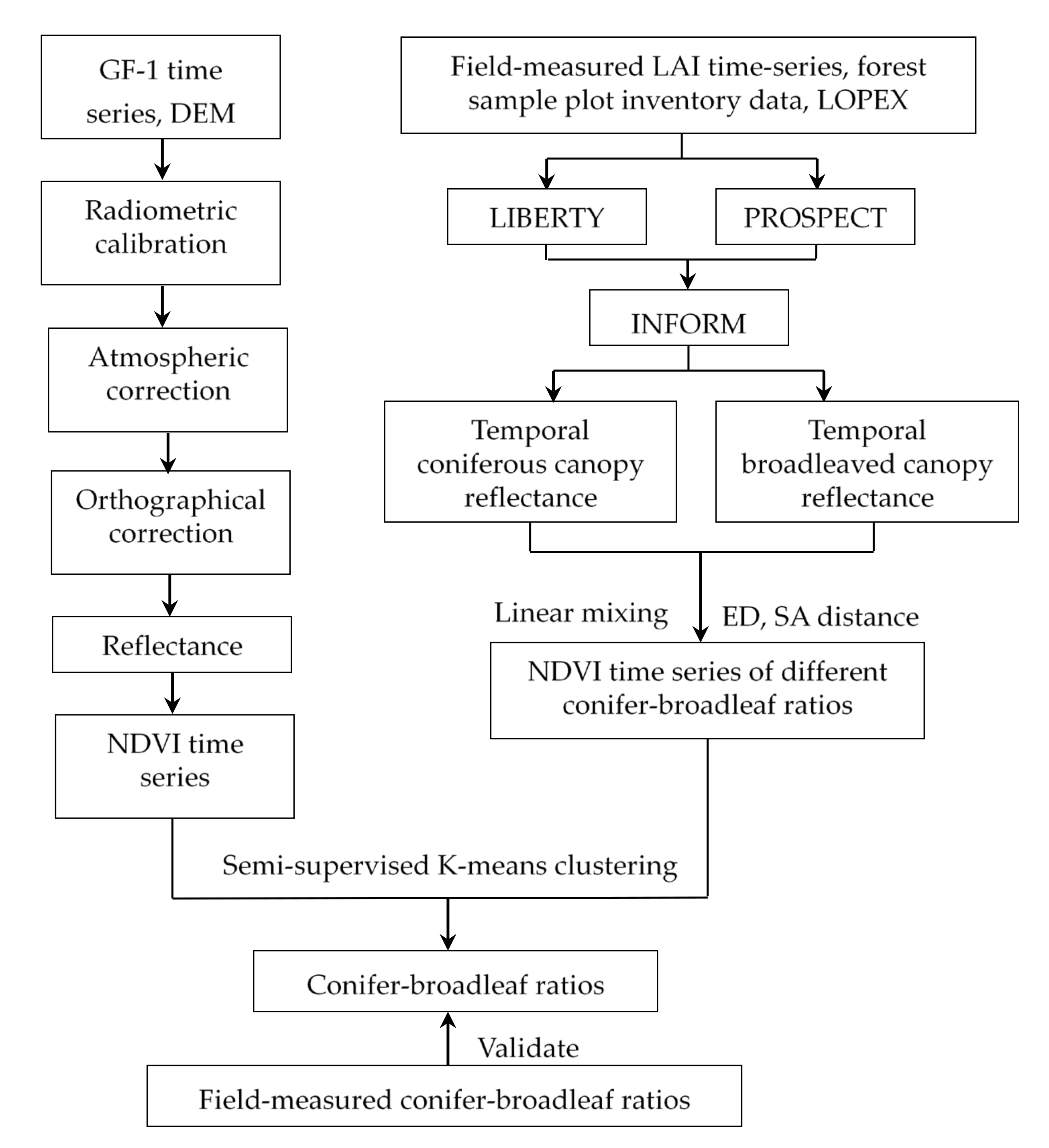
As the first satellite of the civilian high-definition Earth observation satellite (HDEOS) project in China, GaoFen-1 (GF-1) was launched in April 2013 [53,54]. This satellite carries two panchromatic/multispectral (P/MS) and four WFV cameras onboard [53,55]. Each GF-1 WFV sensor has four multispectral bands, ranging from the visible to NIR spectral domains, 450–890 nm, with a spatial resolution of 16 m [53,54,55], as listed in

Table 2. Technical specifications of the GF-1 wide field-of-view (WFV) cameras (Available on the website of China Center For Resources Satellite Data and Application, http://www.cresda.com/CN/Satellite/3076.shtml, accessed on 16 May 2014).

Launch date	26/04/2013
Payloads	WFV
Spatial resolution (m)	16
Wavelength (nm)	Panchromatic: 450–890 nm
	Multispectral	Blue: 450–520 Green: 520–590 Red: 630–690 Near-infrared: 770–890
Swath width (km)	800 (4 cameras combined)
Average orbit height (km)	645
Repetition cycle (day)	4
Orbit inclination/Local time of descending node	98°/11:10 am
Orbit type	Sun-synchronous
Designed lifetime (year)	5–8

. The swath width of the four combined WFV sensors reached 800 km, which theoretically yields a temporal resolution of four days [54]. The decametric spatial resolution, wide coverage ability, and high-frequency revisit time characteristics of GF-1 WFV data render them highly suitable data sources for dynamic vegetation monitoring at a large scale [53,54].

In this study, we obtained a total of 15 cloudless scenes or limited cloud cover images (

Table 3. Information on the acquired GF-1 WFV multi-temporal images and the forest phenology.

Number	Image Acquisition Time	Sensor	Forest Growth Stage
1	01/01/2015	WFV2	dormancy
2	17/01/2015	WFV1	dormancy
3	19/02/2015	WFV1	germination
4	12/03/2015	WFV3	frondescence
5	14/04/2015	WFV3	frondescence
6	22/04/2015	WFV2	frondescence
7	26/04/2015	WFV2	frondescence
8	12/05/2015	WFV1	frondescence
9	21/05/2015	WFV4	frondescence
10	14/06/2015	WFV2	leaf peak
11	02/08/2015	WFV4	leaf peak
12	02/10/2015	WFV1	leaf fall
13	15/10/2015	WFV1	leaf fall
14	01/11/2015	WFV3	leaf fall
15	03/12/2015	WFV2	leaf fall

) of the Purple Mountain area in 2015, from the website of China Center For Resources Satellite Data and Application (http://218.247.138.119:7777/DSSPlatform/productSearch.html, accessed from 2 March 2015 to 26 December 2015). Each month had at least one high-quality image data, except for August and September, which had no clear available image data due to cloud cover during the rainy season. Additionally, a DEM with a spatial resolution of 30 m was acquired for terrain correction in the study area. The DEM was from the second version of the ASTER Global Digital Elevation Model (ASTER GDEM 2) dataset, downloaded from the website (http://datamirror.csdb.cn/index.jsp, accessed on 6 January 2015) in 2015.

The preprocessing of GF-1 satellite WFV data primarily consisted of radiometric calibration, atmospheric correction, and orthographical correction. The spectral response function and absolute radiometric calibration parameters of GF1-WFV data were obtained from the website of the China Resources Satellite Application Center. All GF-1 WFV images were atmospherically corrected to the surface reflectance through the FLAASH Atmospheric Correction module. The orthographical correction was based on the 30 m DEM and forty ground control points (GCPs) recorded in the field using the differential GPS device ensured an accuracy within 0.5 pixels; all operations were conducted on the ENVI/IDL platform.

2.4. Methodology

The estimation of the canopy conifer-broadleaf ratios from the multispectral remote sensing data using the PROSPECT, LIBERTY, and INFORM reflectance models, as well as the semi-supervised K-means clustering algorithm, mainly utilizing the computer workstations, a 64-bit laptop and MATLAB R2015b software (MathWorks, Nattick, MA, USA), consisted of five steps (Figure 3):

(a)

Analyzing model parameter sensitivity and determining the value range of the parameter inputs according to the field measurements of the LAI time-series data, sample plot inventory, and other reference materials.

(b)

Simulating the visible and near-infrared bi-directional spectral reflectance of coniferous and broad-leaved forest canopies using INFORM and calculating the NDVI time-series under different conifer-broadleaf ratios based on the principles of linear mixing.

(c)

Calculation of the Euclidean distance and spectral angle distance between any two NDVI time-series curves of different conifer-broadleaf ratios, analyzing the separability and determining the typical separable ratios.

(d)

Constructing a GF-1 NDVI time-series dataset, from which curves with typical separable ratios were extracted as prior sample data.

(e)

Using the semi-supervised K-means clustering method, obtain the conifer-broadleaf ratio of the study area at the pixel level based on the GF-I NDVI time-series data and evaluate the overall estimation accuracy.

2.4.1. Model Description

INFORM is a hybrid model, combining FLIM, SAILH, and the PROSPECT or LIBERTY submodels, that simulates the bi-directional reflectance of forest stands between 400 and 2500 nm [20,27,56]. For a given band, INFORM calculates the reflectance-based on the principle of FLIM as follows:

$$R=R_C·C+R_G·G$$

(1)

where $R_C$ is the crown reflectance at the infinite crown depth, C is the “crown factor,” $R_G$ is the background reflectance, and G is the “ground factor.” Here, C is calculated as follows:

$$C=\left(1-T_s·T_o\right)·c_s·c_o$$

(2)

where $T_s$ and $T_o$ are the average crown transmittance in the sun and observation directions, respectively, and $c_s$ and $c_o$ are the ground coverage by crowns in the sun direction and the observation direction, respectively.

Here, G is the “ground factor,” which is calculated as follows:

$$G=F_a·T_s·T_o+F_b·T_o+F_c·T_s+F_d$$

(3)

where $F_a$ represents tree crowns with a shadowed background, $F_b$ indicates tree crowns with a sunlit background, $F_c$ is shadowed open space, and $F_d$ is sunlit open space. Atzberger [19] reports the specific calculation formulas for these four fractions. The fractions in Equation (3) are calculated using $c_o$, $c_s$ [Equations (4) and (5)], tree height, CD, illumination, and observation geometry [21].

The $c_o$, under an observation zenith angle of ${\theta }_o$ is given as follows:

$$c_o=1-e^{\frac{-k·SD}{COS\theta o}}$$

(4)

where k is a constant value, SD is the stem density. The k represents the average crown horizontal area, it is calculated as follows:

$$k=\frac{\pi ·{\left(0.5·CD\right)}^2}{10000}$$

(5)

where CD is the crown diameter.

Similar to $c_o$, the observed ground coverage by shadow, $c_s$, under a sun zenith angle of ${\theta }_s$ is given as follows:

$$c_s=1-e^{\frac{-k·SD}{COS\theta s}}$$

(6)

The crown transmittance in the sun direction $T_s$, and observation direction $T_o$ are computed as follows:

$$T_s=f_{SAIL}(LAI,ALA,\tau ,\rho ,{\theta }_s,\psi ,sky1,hot)$$

(7)

$$T_o=f_{SAIL}\left(LAI,ALA,\tau ,\rho ,{\theta }_o,\psi ,sky1,hot\right)$$

(8)

where LAI is the leaf area index, ALA is the average leaf inclination angle, $\tau$ is leaf transmittance, $\rho$ is leaf reflectance, ${\theta }_s$ is solar zenith angle, ${\theta }_o$ is observation zenith angle, $\psi$ is the relative azimuth angle between sun and observer, $sky1$ is the fraction of diffuse radiation, and $hot$ is the hot spot parameter [23].

INFORM computes background reflectance $R_G$ as follows,

$$R_G=f_{SAIL}(LA{I}_U,AL{A}_U,\tau ,\rho ,{\rho }_{soil},{\theta }_o,{\theta }_s,\psi ,sky1,hot)$$

(9)

where $LA{I}_U$, $AL{A}_U$ are the LAI, ALA of the understory vegetation, respectively,${\rho }_{soil}$ is the soil reflectance.

Similar to $R_G$, the crown reflectance at an infinite crown depth, $R_C$ is computed as follows:

$$R_C=f_{SAIL}(LA{I}_{inf},ALA,\tau ,\rho ,{\rho }_{soil},{\theta }_o,{\theta }_s,\psi ,sky1,hot)$$

(10)

where $LA{I}_{inf}$ is the LAI at the infinite crown depth (i.e., LAI ≥ 15).

INFORM can be coupled with the PROSPECT and LIBERTY models for use in deciduous and coniferous forests, respectively. For example, in LIBERTY, $\tau$ is leaf transmittance, $\rho$ is leaf reflectance, they are computed as follows:

$$\tau =f_{LIBERTY}(d,i,t,c_{AB},c_W,c_L,c_P)$$

(11)

$$\rho =f_{LIBERTY}\left(d,i,t,c_{AB},c_W,c_L,c_P\right)$$

(12)

where $d$ is the cell diameter,$i$ is intercellular air space, $t$ is leaf thickness, $c_{AB}$ is chlorophyll content (a + b), $c_W$ is water content, $c_L$ is lignin and cellulose content, $c_P$ is protein content.

In summary, INFORM calculates the forest reflectance, R, as a function of internal canopy parameters, internal leaf parameters, and external parameters as follows:

$$R=f_{INFORM}(SD, CD, H, LAI, ALA, LA{I}_{inf}, LA{I}_U, AL{A}_U, {\rho }_{soil},d,i,t,c_{AB},c_W,c_L,c_P,{\theta }_o,{\theta }_s,\psi ,sky1,hot)$$

(13)

In INFORM, $LA{I}_s$ is the canopy LAI, it is calculated as follows:

$$LA{I}_s=LA{I}_c/CO$$

(14)

where $LA{I}_c$ is a single-tree LAI, Previously, $CO$ was denoted as the “observed ground coverage by crowns ($c_o$)” (Equation (4)), but is now simply referred to as “crown closure.”

For forest vegetation with a high canopy density, the LAI of a single leaf in the model is usually directly equivalent to the $LA{I}_c$. As the study area was Purple Mountain and the forest canopy density was high, the individual tree LAI in the model was also analyzed as the $LA{I}_c$.

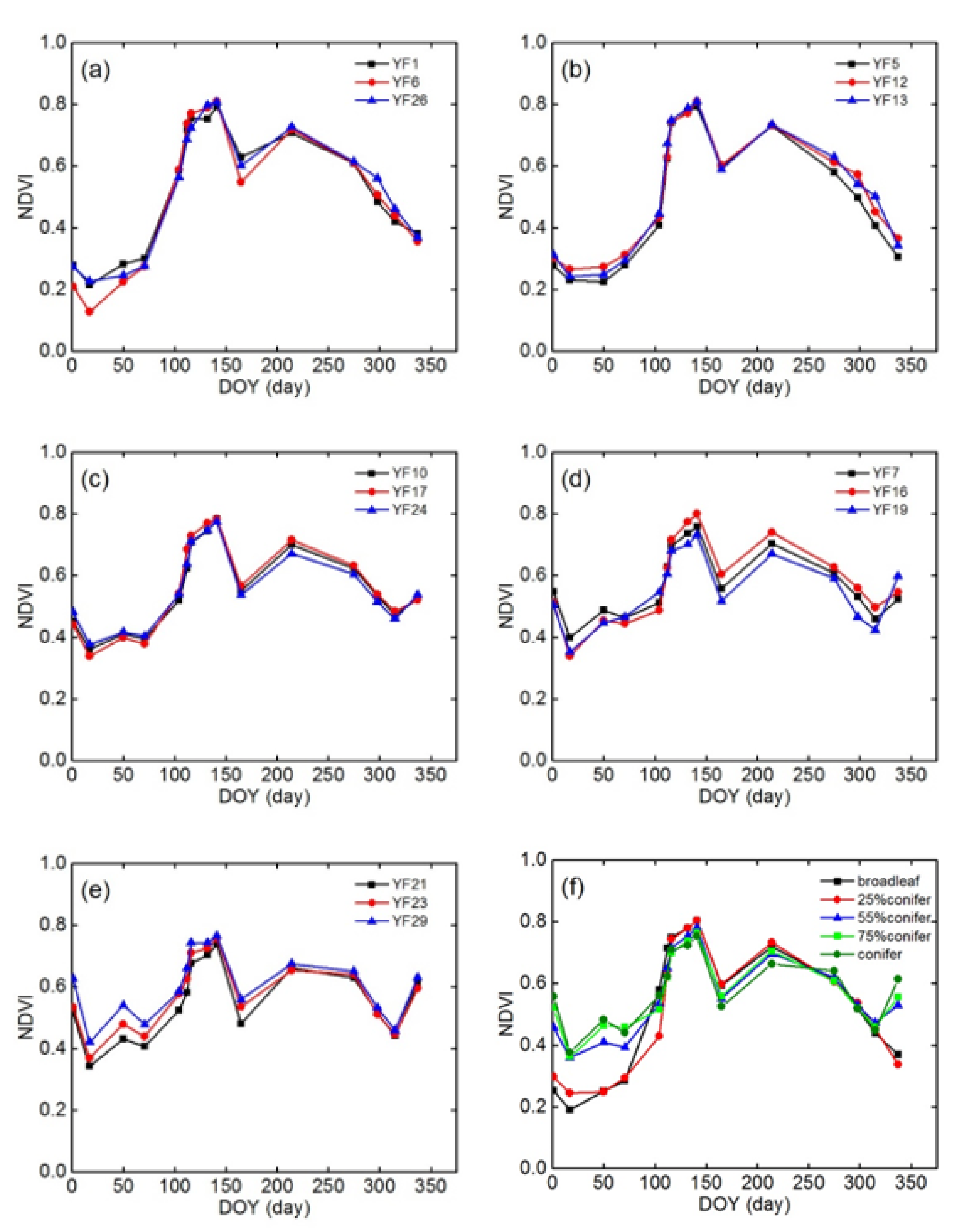
2.4.2. NDVI Time-Series

The NDVI is one of the most commonly used vegetation indices in optical remote sensing, which is based on the intrinsic characteristics of leaf absorbance in the red region and high reflectance in the near-infrared (NIR) region [31,32,33,34,57]. It is highly sensitive to the biochemical and structural composition of the canopy and is characterized by a light computation load [6,31]. The NDVI is calculated as follows:

$$\mathrm{NDVI}=\left({\rho }_{\mathrm{NIR}}-{\rho }_{\mathrm{R}}\right)⁄\left({\rho }_{\mathrm{NIR}}+{\rho }_{\mathrm{R}}\right)$$

(15)

where ${\rho }_{\mathrm{R}}$ and ${\rho }_{\mathrm{NIR}}$ are the reflectance in the red and near-infrared domains, respectively.

Generally, an NDVI time series can be obtained from sequential satellite observations or model simulations. In this study, the satellite-derived NDVI time-series was constructed using the composite data available from the 2015 GF-1 WFV data source, where the temporal NDVI curve of each individual pixel represented the dynamic information for the corresponding vegetation growth over the study period. As the remote sensing images selected here were all clear images with no clouds or reduced clouds, smoothing, filtering, and other processing were not performed for NDVI time-series construction. To ensure correct data acquisition, smoothing and other forms of processing should be avoided to the greatest extent possible to enable more original details to be obtained.

The PROSPECT and LIBERTY leaf models and the INFORM canopy model were combined to simulate broad-leaved and coniferous canopy reflectance across different periods. The simulated canopy reflectance was averaged; the average reflectance of broadleaf and conifer trees in each period was then linearly mixed according to their proportions, with an interval of 5%. The resulting conifer-broadleaf mixing ratios were as follows: pure conifer, 95:5, 90:10, …, 5:95, and pure broadleaf, i.e., 100% conifer, 95% conifer and 5% broadleaf, 90% conifer and 10% broadleaf, …, 5% conifer and 95% broadleaf, and 100% broadleaf. Subsequently, the reflectance obtained after mixing was resampled based on the relative spectral response profiles of the GF-1 WFV sensor. The NDVI sequence data for different conifer-broadleaf ratios were calculated in the range of 300–800 nm.

2.4.3. Similarity Measures for Time-Series

Time-series similarity is usually used to characterize numerically the relationship between time-series data [35]; here it can provide a decision criterion for the discrimination of the NDVI time-series with different conifer-broadleaf ratios. The similarity or difference between the curves can be measured using the numerical value and curve shape. Small numerical differences and similar shapes indicate high similarity; otherwise, the similarity is low. The Euclidean distance (ED) is generally used to quantify the difference in time-series values and spectral angular shapes.

The ED is derived from the distance formula between two points (X1, X2) in an n-dimensional Euclidean space [36]. When applied to similarity analyses of NDVI time-series, the ED measures the overall difference in the numerical value of the NDVI by calculating the distance between the corresponding time ranges of the two time-series curves. The ED was calculated as follows:

$$ED=\sqrt{{\displaystyle \sum }_{i=1}^n{\left(x_i-y_i\right)}^2}$$

(16)

where $x_i$ and $y_i$ are the x and y time-series values at moment i, respectively, and n is the number of samples in the time-series.

Spectral angle-matching algorithms can be used to identify similarity by calculating the spectral angle between the test spectrum and target spectrum. In an n-dimensional space, each spectral curve is a vector with a direction and length, and the included angle that forms between the spectral vectors is the spectral angle (SA) [38,39]. In contrast to the ED, the spectral angle is insensitive to albedo differences [39]. It only measures differences in the spectral shape, with smaller angles indicating more similar spectra. In this study, the NDVI time-series was analogized to a spectrum by calculating the spectral angle distance between the NDVI time-series of different conifer-broadleaf ratios to analyze the separability. The spectral angle (SA) was calculated as follows:

$$\mathrm{SA}\left(\mathrm{x},\mathrm{y}\right)={\cos }^{-1}\left({\sum }_{i=1}^n{x}_i·y_i|\sqrt{{\sum }_{i=1}^n{x}_i^2}·\sqrt{{\sum }_{i=1}^n{y}_i^2}\right)$$

(17)

where $x_i$ and $y_i$ are the x and y time-series values at moment i, respectively, and n is the number of samples in the time-series.

2.4.4. Semi-Supervised K-Means Clustering of NDVI Time-Series

Based on the similarity and dissimilarity of the simulated NDVI time-series with different conifer-broadleaf ratios, semi-supervised clustering analysis can be conducted on NDVI time-series image data to estimate the conifer-broadleaf ratios of the entire study area, with small intra-class differences and large inter-class differences. As a simple but efficient semi-supervised clustering method, the semi-supervised k-means clustering algorithm of time-series improves upon the classic k-means clustering algorithm [58,59]. Traditional k-means clustering aims to partition n observations into k clusters and is widely used for solving time-series data clustering problems [40,41,58]. The main principle of the semi-supervised k-means or k-means clustering algorithm is the minimization of the total distance (typically the ED) between all objects in a cluster from their center [42,58,59,60], where the cluster center is defined as the mean vector in the cluster [41,43]. Before applying the clustering algorithm, the centroid values for the initial clusters and the optimal number of clusters must be predefined, which also determines the final clustering accuracy [40,41,42]. For k-means clustering, k objects are randomly selected as the initial centroid of k clusters [41,58]. Unlike k-means clustering, semi-supervised k-means clustering contains additional supervised information, i.e., some labeled samples [41,59,61]. For these k groups of prior samples, the mean value of each group is directly selected as the initial cluster center, and the k value is the optimal number of clusters [58,59,61].

The process of the semi-supervised k-means clustering algorithm is as follows.:

Step 1.

Define the number of clusters, k, and calculated the initial cluster centers, ${\mu }_i$.

Step 2.

Calculate the ED of objects from ${\mu }_i$.

Step 3.

Obtain the closest cluster to the object and assign the object to that cluster.

Step 4.

Recalculate the cluster means and update the cluster centers.

Step 5.

Recalculate the ED of the objects from the updated cluster centers.

Step 6.

Repeat steps 2–5 until the cluster means do not update.

$${\mu }_i=\frac{1}{S_i}{\displaystyle \sum }_{i=1}^{S_i}{y}_i$$

(18)

where Si represents the number of observations in the ith cluster.

3. Results

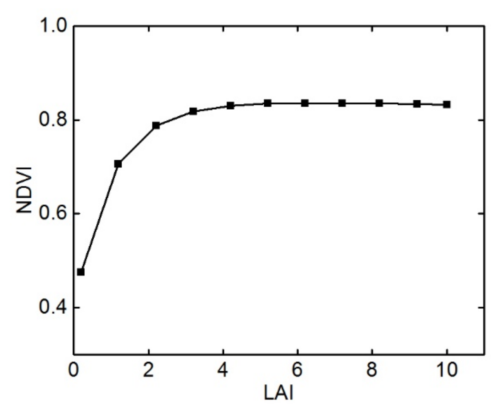
3.1. Sensitivity Analysis and Determination of Model Parameters in Different Growth Periods

In this study, a broad-leaved leaf-level reflectance model (PROSPECT), coniferous leaf-level reflectance model (LIBERTY), and canopy reflectance model (INFORM) were used to simulate the temporal spectral characteristics of broad-leaved and coniferous forests. We adopted parameter sensitivity analysis to analyze the degree of influence and sensitive wavelength range of the different model parameters to the spectral characteristics and more accurately determine the value ranges of the model input parameters. In the sensitivity analysis, when one variable parameter was analyzed, the other variables were set as the constants, and the corresponding spectral reflectance characteristics were simulated.

The simulation results suggested that the broadleaf leaf structure parameter (N) and chlorophyll a + b content (Cab) from the PROSPECT model had a significant influence on the leaf spectral reflectance. The brown pigment content (Cbrown) had a not so significant effect on the near-infrared band, whereas other parameters, such as the equivalent water thickness (Cw), dry matter content (Cm), and carotenoid content (Car), had a negligible influence on the leaf spectral reflectance.

For the INFORM canopy model, parameters such as the LAI_s, standing degree (SD), CD, solar zenith angle (SZA), and observed zenith angle (OZA) all had a significant influence on the canopy spectral characteristics. The SD and CD remained constant during the annual growth cycle, regardless of seasonal variations. The understory leaf area index (LAIU) only had an influence when the forest did not achieve full canopy cover at the beginning of growth. Other parameters, such as relative azimuth angle (RA), ALA, H, and scattering radiation ratio (FDR), had a negligible influence. Among all of the model input parameters, the continuously changing LAI was the most important factor affecting the canopy spectral characteristics.

In summary, we considered all of the values for the input parameters in PROSPECT, i.e., Cab, Cw, Car, and Cm, and those in INFORM, i.e., the LAI, SZA, ALA, and OZA, during the various growth periods; the other parameters were fixed at constant values for the remaining experiments. Among them, the broadleaved leaf parameter input values, except for the ALA, were mainly obtained by referring to the LOPEX database and previous studies [62]. The canopy parameter (e.g., the LAI, LAIU, ALA, SD, H, and CD) inputs were obtained from the measured data, while angle information was obtained from the image header files of GF-1 in each period. For the ALA, we observed that the broadleaved leaves at the germination stage were mostly new and upright during the measurement process; the ALA was large, up to approximately 70°. The leaves continued to grow, such that the ALA decreased to 40°.

Table 4. Input parameters for different growing seasons to analyze the influence of leaf and canopy parameters on the spectrum based on simulation data using the PROSPECT + INFORM model.

	DOY	18	98	116	132	151	190	227	253	271	289	305	320	345
Parameter
Cab		2	6	17	45	70	85	75	40	25	10	8	5	4
Car		4	4	6	7	8	10	10	12	15	18	19	19	18
Cw		0.005	0.007	0.01	0.01	0.02	0.04	0.03	0.02	0.015	0.01	0.008	0.007	0.006
Cm		0.002	0.002	0.003	0.004	0.004	0.004	0.005	0.005	0.006	0.007	0.008	0.008	0.01
N		1.5
Cbrown		0
LAI		0	1–1.5	1.5–2.5	4–5.5	6.5–10	6.5–9	6.5–8	5.5–7.5	4–5.5	3.5–5	2.5–3.5	1.5–2.5	1–2
ALA		40	70	70	60	50	40	25	25	25	25	40	40	40
SZA		35	60	68	71	76	75	62	56	54	50	43	40	35
RA		59	126	47	39	137	52	52	52	60	63	106	52	69
OZA		18	5	3	20	15	28	25	24	24	7	16	15	13
LAIU		0.1–0.5	0.1	0.1	0.1	0.1	0.1	0.1	0.1	0.1	0.1	0.1	0.1	0.1
SD		400
H		15
CD		5
FDR		0.34

lists the values of the broadleaved model parameters for different growth periods.

The results of sensitivity analysis for the parameters of LIBERTY showed that the IAS and CD mainly affected the coniferous leaf spectral reflectance in the visible and near-infrared bands. The albino absorbance (AA) also influenced the leaf reflectance, but it was mainly concentrated in the green band domain. The Cab only had a negligible influence on the reflectance in the visible band. The LT influenced the leaf reflectance in all bands, but mainly in the near-infrared band, whereas the other parameters had almost no influence.

Owing to the lack of measured coniferous leaf biochemical parameters, the ranges of parameters were according to previous studies [26]. Particularly, values of the CD, IAS, and AA were unstable and difficult to measure; most studies have treated these parameters as constant values. Similar to broadleaf, the coniferous canopy structure parameters (e.g., the LAI, LAIU, ALA, SD, H, and CD) were also obtained from the measurements of coniferous trees in the study area.

Table 5. Input parameters for different growing seasons to analyze the influence of leaf and canopy parameters on the spectrum based on simulation data using the LIBERTY + INFORM model.

	DOY	18	98	116	132	151	190	227	253	271	289	305	320	345
Parameters
LT		1.6	1.2	1.4	1.5	1.6	1.6	1.6	1.6	1.6	1.6	1.6	1.6	1.6
Cab		40	45	50	55	60	70	90	75	70	65	60	55	50
Cw		55	60	65	70	75	90	100	100	90	80	70	60	55
LC		70	45	45	45	50	55	60	60	60	60	65	70	70
N		1	1	1	1	1.05	1.15	1.15	1.15	1.15	1.15	1.15	1	1
CD		45
IAS		0.028
B		0.0006
AA		2
LAI		2–4.5	2.5–4.5	3–4.5	3–5	3–5	3–5	3.5–5	3–5	3–5	3–5	3–5	3–5	2.5–4.5
LAIU		0.1	0.5	1	1	1	1	1	1	1	1	0.8	0.5	0.1
ALA		40	70	65	55	45	40	40	40	40	40	40	40	40
SZA		35	60	68	71	76	75	62	56	54	50	43	40	35
RA		59	126	47	39	137	52	52	52	60	63	106	52	69
OZA		18	5	3	20	15	28	25	24	24	7	16	15	13
SD		600
H		20
CD		4
FDR		0.34

lists the values of the coniferous model parameters for different growth periods.

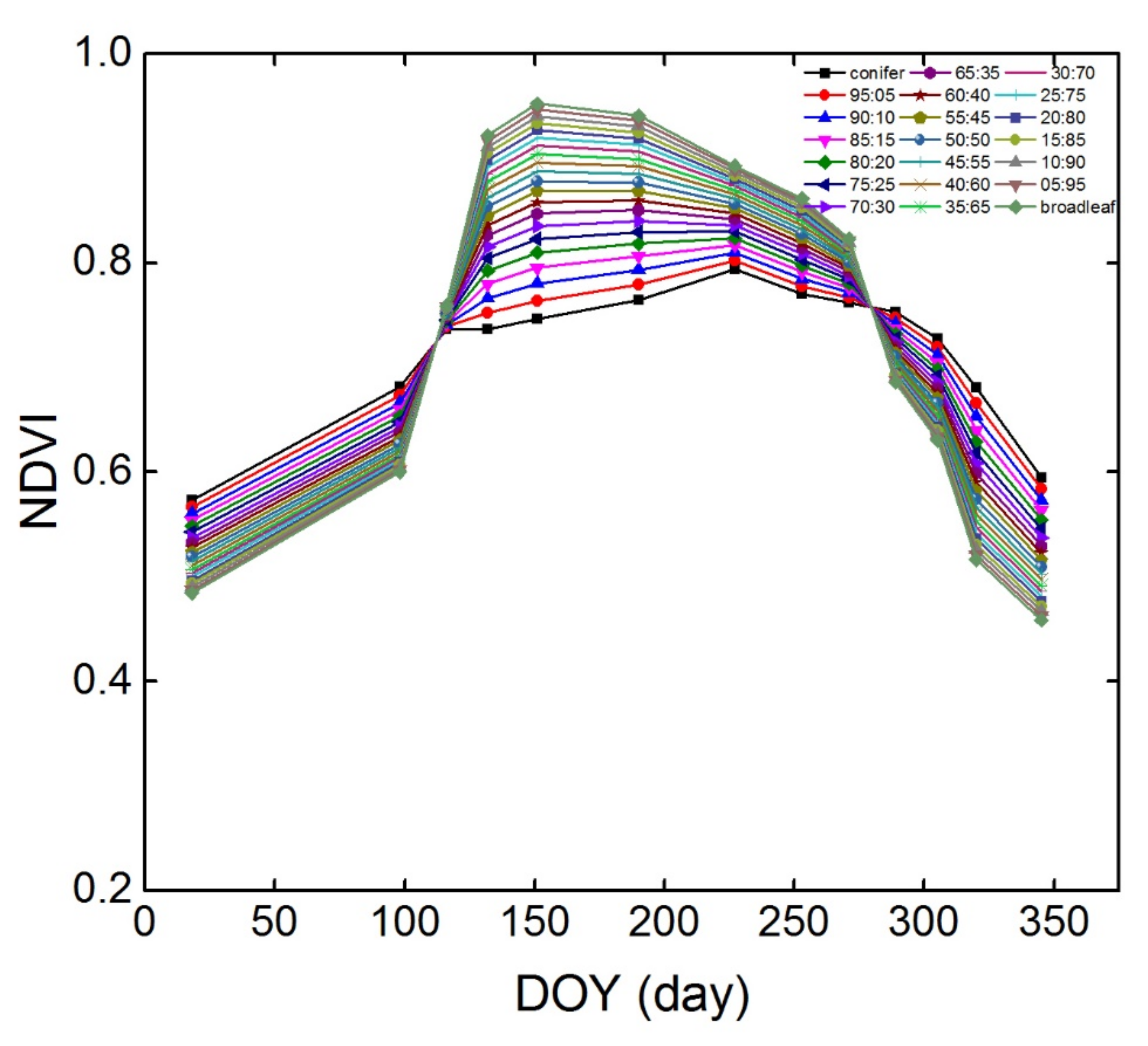
3.2. NDVI Time-Series of Different Conifer-Broadleaf Ratios

The mixed broadleaf-conifer forest in the remote sensing images is essentially a problem with mixed pixels. In this study, we assumed that the pixels were only composed of coniferous and broad-leaved forest types, conforming to the linear mixing principle. Based on the above input parameters (Table 4 and Table 5), the NDVI time-series of different conifer-broadleaf ratios were obtained using the methods described in Section 2.4.2, as shown in Figure 4.

Based on Figure 4, mixed forests with varying conifer-broadleaf ratios presented highly different NDVI temporal profiles due to the variable physiological properties between conifer and broadleaf trees. Except for the intersection points along the curves from DOY98–116 (8–26 April) and DOY271–289 (28 September–16 October), the morphologies and values of the NDVI time-series curves under different conifer-broadleaf ratios all showed differences in the other growing seasons. The pure coniferous canopy had the highest NDVI from both DOY18–98 (18 January–8 April) and DOY289–345 (16 October–11 December): with a decrease in the proportion of the coniferous canopy, there was a corresponding decrease in the NDVI. This was because the dormancy and germination stages of deciduous broad-leaved forests were from 18 January–8 April, as well as the leaf-spreading peak period of coniferous forests; however, the deciduous stage of broad-leaved forests was from 28 September–16 October. Therefore, the LAI of coniferous forests during these two periods was usually larger than that of broad-leaved forests; the corresponding NDVI values were also larger for canopies with more coniferous leaves. During the period from DOY116–271 (26 April–28 September), the NDVI of the pure broadleaf canopy was the largest; the NDVI of the corresponding broadleaf canopy decreased with an increasing proportion of conifers. The main reason for this is that this was the peak leaf-spreading period of broadleaved and coniferous forests. As the leaf-spreading rate of the broad-leaved forest was higher, the canopy LAI and NDVI both increased rapidly; their values were generally greater than those of the coniferous canopy.

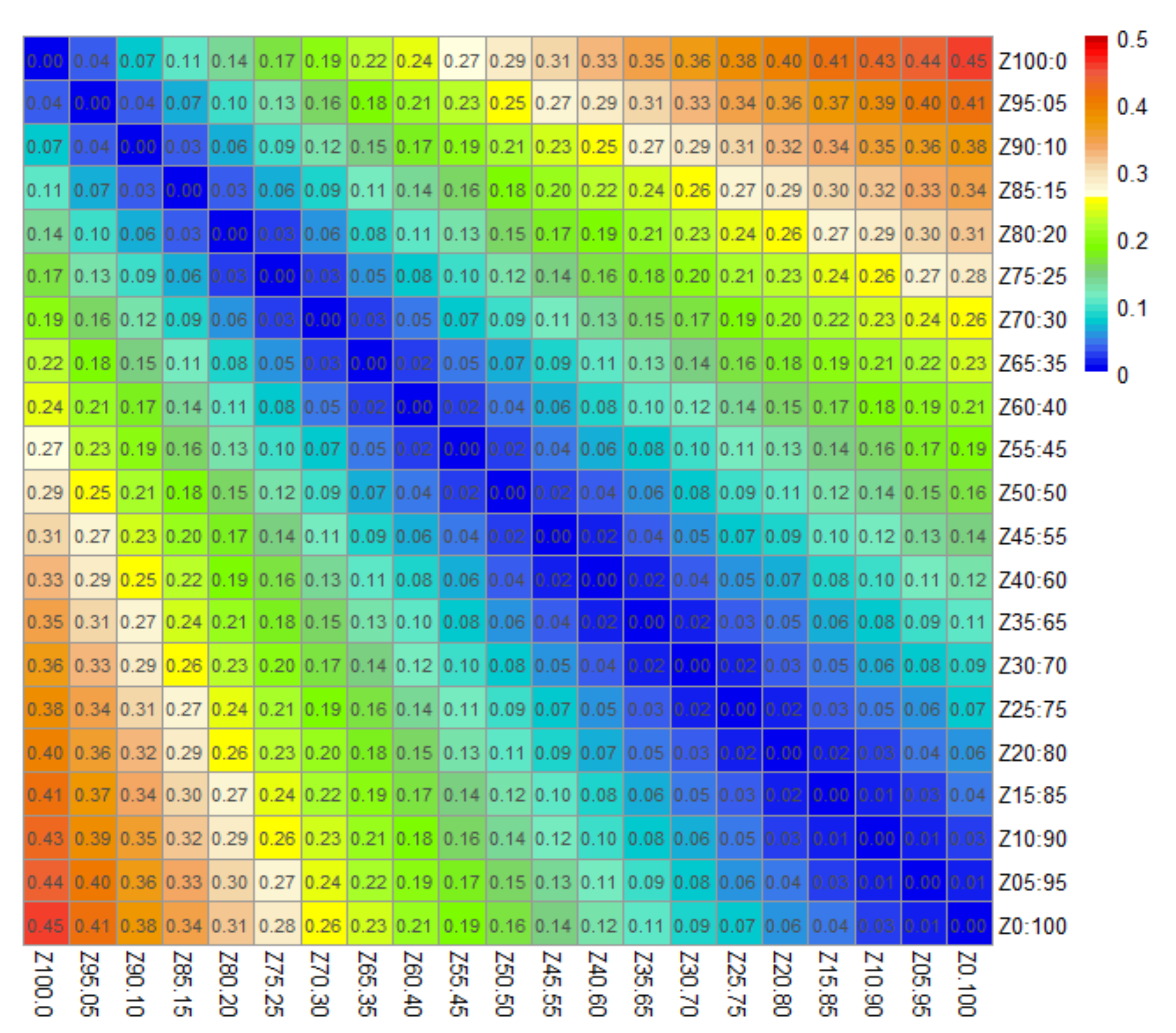
3.3. Calculation of ED and SA Distance

According to the simulation results in Section 3.2 for the NDVI time-series of different conifer-broadleaf ratios, the ED and SA distances were calculated using the R language, and heatmaps of the calculation matrix were drawn using the Pheatmap program package, as shown in Figure 5.

According to Section 2.4.3, the larger the ED value of the NDVI time-series with different conifer-broadleaf ratios, the greater the difference between them, indicating the higher separability between the two ratios. Based on Figure 5, the maximum distance was 0.45, which corresponds to the distance between the curves of pure conifer and pure broadleaf, implying that they had significant separability. A minimum distance of 0 was the value between the two curves with equivalent conifer-broadleaf ratios. Based on the difference in the distance values, the twenty-one conifer-broadleaf ratios could be divided into ranges that were significantly different from each other. The separation criteria were as follows: distance values within each range were relatively approximate, i.e., high similarity and low separability in the NDVI time-series between corresponding conifer-broadleaf ratios, and distance values between ranges differed significantly, with substantial separability. An analysis of the distance value in Figure 5 indicates that the ED between the NDVI time-series of different conifer-broadleaf ratios presented four aggregation intervals, according to their degree of difference, as reflected in the different colors displayed in the heat map. Taking the values in the right-most column as an example, i.e., the Euclidean distance between the NDVI time-series of pure broadleaf and other conifer-broadleaf ratios, the value domains were 0.28–0.45, 0.16–0.28, 0.07–0.16, and 0–0.07.

Obviously, the conifer-broadleaf ratios corresponding to the boundary values of each distance interval were the significant separability ratios. There were pure conifer (100% conifer), 75% conifer and 25% broadleaf, 50% conifer and 50% broadleaf, 25% conifer and 75% broadleaf, and pure broadleaf (100% broadleaf). Accordingly, the significant separable range in the study area could be described by the following ranges according to the conifer proportions: conifer, conifer–75% conifer, 75–50% conifer, 50–25% conifer, 25% conifer-broadleaf (hereinafter referred to as conifer, ~75% conifer, ~50% conifer, ~25% conifer, and broadleaf).

The ED only reflects the difference between the NDVI time-series curves with different conifer-broadleaf ratios from the perspective of the NDVI values. To fully consider the discriminability of the feature vector from the NDVI time-series, we analyzed the difference in the curve shape, which was evaluated by the SA distance. According to the methods described in Section 2.4.3, Figure 6 shows the calculation results.

Based on Figure 6, the value of SA distance was generally greater than that of ED, with a range of 0–9.42, indicating that the morphological differences in the NDVI time-series curves under different ratios were more significant than those of the NDVI values.

Similar to the ED results, the SA distance values in Figure 6 also show four aggregation intervals according to their degree of difference. The SA distance value domains of the corresponding conifer-broadleaf ratios were 0–1.44, 1.44–3.3, 3.3–5.83, and 5.83–9.42, taking the values in the right-most column as an example. There were large differences between the different ranges; the differences in the values within each range were small, which further verified the conclusions obtained based on the ED, i.e., the twenty-one different conifer-broadleaf ratios could be divided into conifer, ~75% conifer, ~50% conifer, ~25% conifer, and broadleaf.

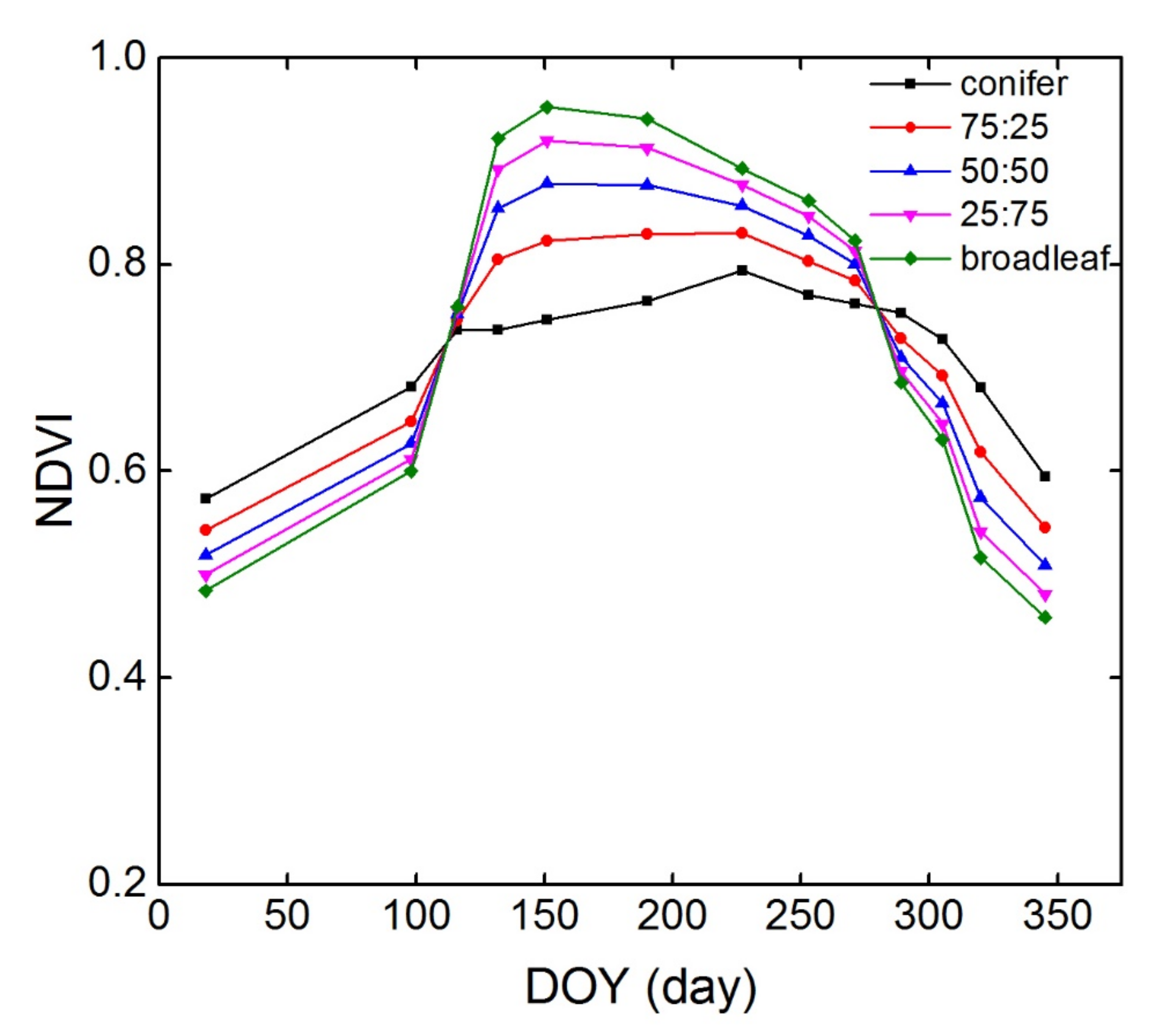
3.4. NDVI Time-Series of Typical Conifer-Broadleaf Ratios

Based on the analysis in Section 3.2 and Section 3.3, the simulated average values of NDVI in each range, namely, conifer, ~75% conifer, ~50% conifer, ~25% conifer, and broadleaf, were calculated as the representative NDVI time-series, as shown in Figure 7.

For the construction of the satellite-derived NDVI time-series, composite data available from the 2015 GF-1 WFV data source were used in this study. The sample plots corresponding to typical conifer-broadleaf ratios can be extracted from remote sensing images, followed by the calculation of the corresponding average NDVI time-series, as shown in Figure 8.

Based on Figure 8, the NDVI time-series curves under different conifer-broadleaf ratios all showed the lowest NDVI value for the entire year on DOY17 (17 January) and the highest value on DOY141 (21 May).

Additionally, the curves corresponding to each ratio range exhibited a substantial decrease in June. During this period (DOY165, 14 June), the cloud-free GF-1 image had a high quality, but the calculated NDVI value was lower overall. A possible reason for this is that the vegetation in the study area had a large blooming area. Owing to the high species diversity in the study area, some tree species, such as Acacia trees (blooming period from April–June), Dalbergia hupeana (blooming period from May–October), Camptotheca acuminata (blooming period from May–July), Elm trees (blooming period of 3–6 months), and Castanopsis sclerophylla (blooming period from May–June), among others, could have been blossoming in June. Specifically, broadleaved sample plots, as shown in Figure 8a,b were dominated by Quercus and Liquidambar formosana, whose leaves began to change color and then fell in September, with a corresponding decrease in the NDVI values. In the three ratio ranges with a conifer ratio ≥ 50%—Figure 8c–e—the NDVI value decreased on DOY104 (14 April) owing to litter replacement with needles, i.e., old leaves fell off of trees and new leaves began to germinate. For the increasing NDVI value on DOY337 (3 December), the influence of understory vegetation disappeared during this period, whereas the influence of needles became observable. From Figure 8f, the NDVI mean curve exhibited a significant difference under typical varying conifer-broadleaf ratios, which could provide samples for the estimation of the conifer-broadleaf ratio.

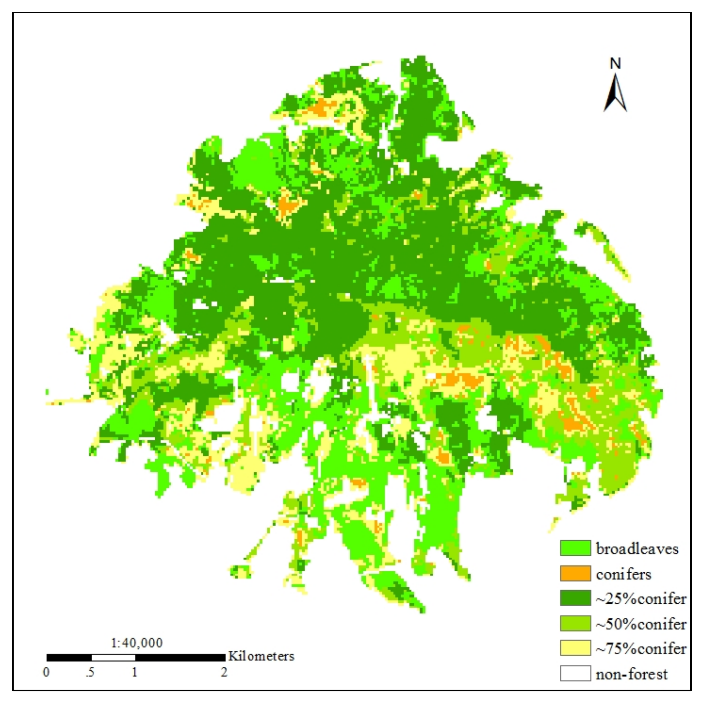
3.5. Conifer-Broadleaf Ratio Estimation Based on Time-Series

According to the above results, we obtained the annual NDVI time-series curves based on prior knowledge, including the five conifer-broadleaf ratios determined through model simulation and the corresponding “standard reference curves”. In this study, the proportions of the different conifer and broadleaf components in mixed forests were distinguished at the pixel level.

Therefore, the NDVI values calculated from the 15 GF-1 images of the study area were stacked to form a new image, i.e., a “multispectral image” with 15 “bands” based on an analogy of the time dimension to the spectral dimension. According to the forest subcompartment map, high-resolution images, and field observations, the non-forest areas in the image were removed by a mask. Then, the semi-supervised k-means clustering method was applied to estimate the conifer-broadleaf ratios at the pixel level for the entire study area, and also to improve the estimation accuracy. Figure 9 shows the estimated results.

Based on Figure 9, the area of the broadleaf-conifer ratio in the range “~25% conifer” was the largest (approximately 8.66 km²) and the corresponding region was mainly distributed in the middle and northern areas of Purple Mountain. The area that the pure broad-leaved forest occupied was 5.47 km², which was mainly distributed in peripheral regions at the foot of Purple Mountain. The areas of broadleaf-conifer ratio ranges “~50% conifer” and “~75% conifer” were approximately equal, 3.42 km² and 3.36 km², respectively, and the corresponding regions were scattered in the southeast and around the foot of the mountain. The area of pure coniferous forest was the smallest, only 0.48 km², and mainly distributed in the vicinity of Linggu Temple and at the top of the north slope of the mountain.

The accuracy of the result map was evaluated based on the conifer-broadleaf ratio data measured at 32 sample plots, the forest survey information from the forest subcompartment map of Purple Mountain, and the Google Earth maps. Eighty samples covering different conifer-broadleaf ratios were selected and compared with the clustering results. Sixty-seven samples fell into the corresponding level, with an overall accuracy (OA) of 83.75%. The kappa coefficient, calculated based on the confusion matrix, was 0.79. The misjudgment mainly occurred when coniferous forests occupied a larger proportion, such as the broadleaf-conifer ratio ranges of “~75% conifer” and pure conifer. As the LAI of coniferous forest was relatively high throughout the year, and the corresponding NDVI value was also higher, which would cover up the growth curve characteristics of deciduous broad-leaved forests to a certain extent.

4. Discussion

4.1. Parameter Sensitivity Analysis

In this study, the leaf reflectance models (PROSEPECT and LIBERTY) and canopy reflectance model (INFORM) were coupled to simulate the broadleaved and coniferous canopy spectral characteristics during different growth periods. The first task was to conduct the parameter sensitivity analysis, which is important to investigate the effects of model parameter variables on reflectance signatures. As the study was based on multispectral time-series analysis, during parameter sensitivity analysis of the INFORM, a comparative analysis of the canopy spectral reflectance was less evident than the analysis of the calculated vegetation indices. Therefore, to quantitatively and more effectively display the influence of different parameters in INFORM on the canopy spectral characteristics, the spectral response functions of the GF-1 WFV remote sensing images were used for resampling based on canopy reflectance simulations, and more commonly used VIs, such as the NDVI, were further calculated.

Additionally, when the INFORM model was used to simulate the temporal canopy reflectance and NDVI to analyze the influence of the model parameters, we found that the LAI was the most important influential parameter. Different from the single-period studies, this study was based on the whole growing season (across the year). Considering the season changes, although other variable parameters, such as ALA, SZA, RA, OZA, and LAIU, also have some certain effects, compared with LAI, their effects are all smaller than the changes caused by LAI. Therefore, to ensure the high accuracy of the simulation results, it is very critical to obtain the LAI measurements of different periods in the study area.

4.2. The NDVI Time-Series

As the most widely used vegetation indices, the NDVI is usually considered as the best indicator of vegetation coverage and the status of vegetation growth [31,39] and is closely related to LAI. However, based on the principle of the NDVI construction, the contrast of NIR and R reflectance is enhanced by nonlinear stretching, and the low-value part of NDVI is enhanced, while the high-value part is suppressed. As a result, the NDVI also suffers from well-known issues, such as saturation at moderate LAI levels (LAI > 3–4) and insensitivity to changes in high biomass conditions [63,64]. In this study, the broadleaved LAI measurement of the study area ranged from 0 to 10, while that of the coniferous LAI ranged from 2 to 5. The correlation between the LAI and NDVI was simulated based on INFORM (Figure 10), to analyze the influence of the canopy LAI on NDVI. As can be seen from Figure 10, when the value of LAI was 4.2, NDVI was 0.83, approximately reaching its maximum value of 0.84. Since then, as LAI gradually increased, while the NDVI remained almost unchanged; which would affect the discrimination of the NDVI time-series with different conifer-broadleaf ratios to some extent.

According to the definition of the conifer-broadleaf ratio, i.e., the relative ratio of the maximum spreading leaf area during vertical observations at the pixel scale, our main concern is the growth and change of green leaves in mixed broadleaf-conifer forests during the growing season throughout the year; which is represented by the NDVI time-series in the remote sensing images. The non-green parts, such as some parts of the forest at a given time might be non-green or non-photosynthetic (e.g., brown/yellow/dead) due to various reasons, were not specially considered. As the NDVI effectively highlights green vegetation, low NDVI values in remote sensing images are usually displayed to show the non-green parts.

4.3. Conifer-Broadleaf Ratios

The conifer-broadleaf ratio discussed in this paper is only applicable to dense forests, i.e., where the canopy is almost closed, broadleaved forests in addition to coniferous forests exist in the pixels, and evergreen broadleaf and deciduous conifers are not considered. Additionally, although the conifer-broadleaf ratio remained constant throughout the year, it could not be estimated based on single-phase images. This is because the spectral characteristics corresponding to different conifer-broadleaf ratios in a single image were highly similar. Effectively distinguishing the spectral characteristics is difficult, especially in multispectral remote sensing studies. Therefore, temporal variations in VI characteristics, such as the NDVI, were considered because the composition of conifers and broad-leaved trees, as well as their temporal variation, in a pixel, was different.

Furthermore, under the same conifer-broadleaf ratio, the time-series curves may be inconsistent due to different tree species and growth conditions. For example, different starting and ending times in the growth periods and growth rates would lead to a shift in the curves extracted from different pixels. Different canopy sizes and tree densities would lead to the oscillation of the corresponding curves, i.e., “different curves in the same ratio.”

However, based on the simulation analysis results, the continuously changing LAI was the most important factor affecting the canopy spectral characteristics. The time-series curves of the NDVI under different LAIs were generally similar in shape, but the values were different. Therefore, the average NDVI time-series curves can be used to represent common characteristics for analysis and research. As the difference between the curves of different conifer-broadleaf ratios varied, whether the separability was significant was related to if it could be accurately reflected and quantitatively expressed by remote sensing images. Therefore, considering the detailed distinction within the coniferous and broad-leaved mixed forests to the greatest extent possible, we must simultaneously consider the discrimination ability of the data.

To better distinguish different conifer-broadleaf ratios and select the ratios with greater differences, we classified twenty-one different conifer-broadleaf ratios and determined the “standard/reference time-series curve” corresponding to each ratio by accounting for dual differences in the shape and distance between the curves. Based on this, we used the ED and SA distances as the separability criteria. The time-series “spectrum” was analogous to the remote sensing spectrum, comprehensively using the spectral and time-series spectrum analysis methods for reference.

This study was based on the time-series curve of the study period, which required high-quality annual images. If a large number of images are missing due to clouds and precipitation in a certain year, constructing the time-series data for that year is impossible. Moreover, this study only conducted a 1-yr time-series analysis; temporal sequence curves will be offset owing to the influence of rainfall, temperature, and other factors between different years.

5. Conclusions

We obtained and analyzed time-series dynamic information of a mixed forest canopy based on field observations and INFORM simulation data, the time-series spectral response characteristics of the coniferous and broad-leaved forest, and the VI time-series characteristics under different conifer-broadleaf ratios. Time-series similarity analysis was employed to determine the five separable ranges of conifer-broadleaf ratios: pure broadleaf, ~25% conifer, ~50% conifer, ~75% conifer, and pure conifer. We proposed a method to estimate the conifer-broadleaf ratio of the horizontal canopy at Purple Mountain. The semi-supervised K-means clustering method was used to estimate the conifer-broadleaf ratio at sub-pixel scales based on 2015 GF-1 NDVI time-series data; an overall estimation accuracy of 83.75% was obtained. We provide a solution to overcome the limitations posed by pixel heterogeneity in mixed forests, and it was of great significance to improve the inversion accuracy of vegetation parameters. In addition, the accurate acquisition of the canopy horizontal composition information, i.e., conifer-broadleaf ratios, is imperative for sustainable forest management in mixed forests, which have rich species diversity, stable ecosystem function, and obvious ecological advantages when compared with pure forests.

Our findings have the potential for widespread application, but they also have some limitations, and future studies should consider the following three topics. First, in view of the inconsistencies in time-series curves, which are caused by differences in phenology and growth periods in various tree species, more data sources, such as high spatial resolution and hyperspectral data, should be used to analyze the differences among specific tree species. Second, due to the limitations of various conditions, only a 1-yr time-series observation was conducted in this study; an appropriate mixed forest growth model should be considered to analyze the time-series characteristics in different years. Finally, for the impact of the spatial distribution of trees, LiDAR data can be used to obtain spatial distribution information on trees in the future.

References

1. Canadian Council of Forest Ministers. Criteria and Indicators of Sustainable Forest Management in Canada: National Status. 2000. Available online: https://d1ied5g1xfgpx8.cloudfront.net/pdfs/18104.pdf (accessed on 6 April 2020).
2. Brown, S. Measuring carbon in forests: Current status and future challenges. Environ. Pollut. 2002, 116, 363–372. [Google Scholar] [CrossRef]
3. Ustin, L.S. Remote sensing of canopy chemistry. Proc. Natl. Acad. Sci. USA 2013, 110, 804–805. [Google Scholar] [CrossRef] [PubMed] [Green Version]
4. Krzystek, P.; Serebryanyk, A.; Schnörr, C.; Červenka, J.; Heurich, M. Large-scale mapping of tree species and dead trees in šumava national park and bavarian forest national park using lidar and multispectral imagery. Remote Sens. 2020, 12, 661. [Google Scholar] [CrossRef] [Green Version]
5. Porté, A.; Bartelink, H. Modelling mixed forest growth: A review of models for forest management. Ecol. Model. 2002, 150, 141–188. [Google Scholar] [CrossRef]
6. Ollinger, S.V.; Reich, P.B.; Frolking, S.; Lucie, C.; Lepinea, D.Y.; Hollingerd, A.D.; Richardsone, A.D. Nitrogen cycling, forest canopy reflectance, and emergent properties of ecosystems. Proc. Natl. Acad. Sci. USA 2013, 110, 2437. [Google Scholar] [CrossRef] [Green Version]
7. Asner, G.P.; Martin, R.E. Spectral and chemical analysis of tropical forests: Scaling from leaf to canopy levels. Remote Sens. Environ. 2008, 112, 3958–3970. [Google Scholar] [CrossRef]
8. Rautiainen, M.; Stenberg, P.; Nilson, T.; Kuusk, A. The effect of crown shape on the reflectance of coniferous stands. Remote Sens. Environ. 2004, 89, 41–52. [Google Scholar] [CrossRef]
9. Knyazikhin, Y.; Schull, M.A.; Stenberg, P.; Mõttusd, M.; Rautiainenc, M.; Yanga, Y.; Marshake, A.; Carmonaf, P.L.; Kaufmanna, R.K.; Lewisg, P.; et al. Hyperspectral remote sensing of foliar nitrogen content. Proc. Natl. Acad. Sci. USA 2013, 110, E185–E192. [Google Scholar] [CrossRef] [Green Version]
10. Wang, Q.; Ding, X.; Tong, X.; Atkinson, M.P. Spatio-temporal spectral unmixing of time-series images. Remote Sens. Environ. 2021, 259, 112407. [Google Scholar] [CrossRef]
11. Abdollahnejad, A.; Panagiotidis, D. Tree species classification and health status assessment for a mixed broadleaf-conifer forest with UAS multispectral imaging. Remote Sens. 2020, 12, 3722. [Google Scholar] [CrossRef]
12. Burchard-Levine, V.; Nieto, H.; Riañoa, D.; Migliavacca, M.; El-Madany, T.S.; Guzinskie, R.; Carrara, A.; Martín, P.M. The effect of pixel heterogeneity for remote sensing based retrievals of evapotranspiration in a semi-arid tree-grass ecosystem. Remote Sens. Environ. 2021, 260, 112440. [Google Scholar] [CrossRef]
13. Zhang, C.; Ma, L.; Chen, J.; Rao, H.Y.; Zhou, Y.; Chen, X.H. Assessing the impact of endmember variability on linear spectral mixture analysis (LSMA): A theoretical and simulation analysis. Remote Sens. Environ. 2019, 235, 111471. [Google Scholar] [CrossRef]
14. Chen, J.M.; Black, T.A.; Adams, R.S. Evaluation of hemispherical photography for determining plant area index and geometry of a forest stand. Agric. For. Meteorol. 1991, 56, 129–143. [Google Scholar] [CrossRef]
15. Zou, T.Y.; Zhang, J. A New fluorescence quantum yield efficiency retrieval method to simulate chlorophyll fluorescence under natural conditions. Remote Sens. 2020, 12, 4053. [Google Scholar] [CrossRef]
16. Chen, J.M. Spatial scaling of a remotely sensed surface parameter by contexture. Remote Sens. Environ. 1999, 69, 30–42. [Google Scholar] [CrossRef]
17. Li, X.W.; Strahler, A.H.; Woodcock, C.A. Hybrid geometric optical-radiative transfer approach for modeling albedo and directional reflectance of discontinuous canopies. IEEE Trans. Geosci. Remote Sens. 1995, 33, 466–480. [Google Scholar] [CrossRef]
18. Liang, L.; Di, G.; Yan, J.; Qiu, S.; Di, L.; Wang, S.; Xu, L.; Wang, L.; Kang, J.; Li, L. Estimating crop LAI using spectral feature extraction and the hybrid inversion method. Remote Sens. 2020, 12, 3534. [Google Scholar] [CrossRef]
19. Atzberger, C. Development of an invertible forest reflectance model: The INFOR-Model. A Decade of Trans-European Remote Sensing Cooperation. In Proceedings of the 20th EARSeL Symposium, Dresden, Germany, 14–16 June 2000. [Google Scholar]
20. Schlerf, M.; Atzberger, C. Inversion of a forest reflectance model to estimate structural canopy variables from hyperspectral remote sensing data. Remote Sens. Environ. 2006, 100, 281–294. [Google Scholar] [CrossRef]
21. Rosema, A.; Verhoef, W.; Noorbergen, H.; Borgesius, J. A new forest light interaction model in support of forest monitoring. Remote Sens. Environ. 1992, 42, 23–41. [Google Scholar] [CrossRef]
22. Verhoef, W. Light scattering by leaf layers with application to canopy reflectance modeling: The SAIL model. Remote Sens. Environ. 1984, 16, 125–141. [Google Scholar] [CrossRef] [Green Version]
23. Verhoef, W. Earth observation modeling based on layer scattering matrices. Remote Sens. Environ. 1985, 17, 165–178. [Google Scholar] [CrossRef] [Green Version]
24. Jacquemoud, S.; Baret, F. PROSPECT: A model of leaf optical properties spectra. Remote Sens. Environ. 1990, 34, 75–91. [Google Scholar] [CrossRef]
25. Jacquemoud, S.; Ustin, S.L.; Verdebout, J.; Schmuck, G.; Andreoli, G.; Hosgood, B. Estimating leaf biochemistry using the prospect leaf optical properties model. Remote Sens. Environ. 1996, 56, 194–202. [Google Scholar] [CrossRef]
26. Dawson, T.P.; Curran, P.J.; Plummer, S.E. LIBERTY-Modeling the effects of leaf biochemical concentration on reflectance spectra. Remote Sens. Environ. 1998, 65, 50–60. [Google Scholar] [CrossRef]
27. Yuan, H.; Ma, R.; Atzberger, C.; Li, F.; Loiselle, S.A.; Luo, J. Estimating forest fapar from multispectral landsat-8 data using the invertible forest reflectance model INFORM. Remote Sens. 2015, 7, 7425–7446. [Google Scholar] [CrossRef] [Green Version]
28. Yang, G.J.; Huang, W.J.; Wang, J.H.; Xing, Z.R. Inversion of forest leaf area index calculated from multi-source and multi-angle remote sensing data. Chin. Bull. Bot. 2010, 45, 566–578. [Google Scholar]
29. Zhang, L.; Zhao, J.L.; Jia, K.; Li, X.S. Research on plant spectral recognition method based on phenological features. Spectrosc. Spectr. Analysis. 2015, 10, 2836–2840. [Google Scholar]
30. Huang, X.; Zhu, W.; Wang, X.; Zhan, P.; Liu, Q.; Li, X.; Sun, L. A method for monitoring and forecasting the heading and flowering dates of winter wheat combining satellite-derived green-up dates and accumulated temperature. Remote Sens. 2020, 12, 3536. [Google Scholar] [CrossRef]
31. Rouse, J.W.; Haas, R.H.; Schell, J.A.; Deering, D.W. Monitoring Vegetation Systems in the Great Plains with ERTS-1, Third Earth Resources Technology Satellite Symposium 1; NASA: Wasgington, DC, USA, 1974; pp. 309–317. [Google Scholar]
32. Dobrinić, D.; Gašparović, M.; Medak, D. Sentinel-1 and 2 time-series for vegetation mapping using random forest classification: A case study of Northern Croatia. Remote Sens. 2021, 13, 2321. [Google Scholar] [CrossRef]
33. López-Amoedo, A.; Álvarez, X.; Lorenzo, H.; Rodríguez, J.L. Multi-temporal Sentinel-2 data analysis for smallholding forest cut control. Remote Sens. 2021, 13, 2983. [Google Scholar] [CrossRef]
34. Chamberlain, D.A.; Phinn, S.R.; Possingham, H.P. Mangrove forest cover and phenology with landsat dense time series in central queensland, Australia. Remote Sens. 2021, 13, 3032. [Google Scholar] [CrossRef]
35. Lhermitte, S.; Verbesselt, J.; Verstraeten, W.W.; Coppin, P. A comparison of time series similarity measures for classification and change detection of ecosystem dynamics. Remote Sens. Environ. 2011, 115, 3129–3152. [Google Scholar] [CrossRef]
36. Lambin, E.F.; Strahlers, A.H. Change-vector analysis in multitemporal space: A tool to detect and categorize land-cover change processes using high temporal-resolution satellite data. Remote Sens. Environ. 1994, 48, 231–244. [Google Scholar] [CrossRef]
37. Gong, X.; Richman, M.B. On the application of cluster analysis to growing season precipitation data in North America east of the rockies. J. Clim. 1995, 8, 897–931. [Google Scholar] [CrossRef] [Green Version]
38. Kruse, F.A.; Lefkoff, A.B.; Boardman, J.W.; Heidebrecht, K.B.; Shapiro, A.T.; Barloon, P.J.; Goetz, A.F.H. The spectral image processing system (SIPS)—Interactive visualization and analysis of imaging spectrometer data. Remote Sens. Environ. 1993, 44, 145–163. [Google Scholar] [CrossRef]
39. Diao, C.; Wang, L. Landsat time series-based multiyear spectral angle clustering (MSAC) model to monitor the inter-annual leaf senescence of exotic saltcedar. Remote Sens. Environ. 2018, 209, 581–593. [Google Scholar] [CrossRef]
40. Aghabozorgi, S.; Shirkhorshidi, A.S.; Wah, T.Y. Time-series clustering—A decade review. Inf. Syst. 2015, 53, 16–38. [Google Scholar] [CrossRef]
41. Zhou, Z.H. Machine Learning; Tsinghua University Press: Beijing, China, 2016; pp. 307–309. ISBN 978-7-302-206853-6. [Google Scholar]
42. Xing, X.; Yan, C.; Jia, Y.; Jia, H.; Lu, J.; Luo, G. An effective high spatiotemporal resolution ndvi fusion model based on histogram clustering. Remote Sens. 2020, 12, 3774. [Google Scholar] [CrossRef]
43. Santos, L.A.; Ferreira, K.; Picoli, M.; Camara, G.; Zurita-Milla, R.; Augustijn, E.W. Identifying spatiotemporal patterns in land use and cover samples from satellite image time series. Remote Sens. 2021, 13, 974. [Google Scholar] [CrossRef]
44. Yan, W.J.; Kong, F.H.; Yin, H.W.; Sun, C.F.; Xu, F.; Li, W.C.; Zhang, X.T. Factors affecting the cooling effect in zijin mountain forest park. Acta Ecol. Sin. 2014, 34, 3169–3178. [Google Scholar]
45. Li, M.S.; Peng, S.K.; Zhong, H.Y. Landscape pattern and dynamic analysis of zijin mountain scenic area based on GIS. J. Nanjing For. Univ. 2004, 5, 67–70. [Google Scholar]
46. Deng, S.; Katoh, M.; Guan, Q.; Yin, N.; Li, M. Interpretation of forest resources at the individual tree level at purple mountain, Nanjing City, China, using worldview-2 imagery by combining GPS, RS and GIS Technologies. Remote Sens. 2014, 6, 87–110. [Google Scholar] [CrossRef] [Green Version]
47. Deng, S.; Katoh, M.; Guan, Q.; Yin, N.; Li, M. Estimating forest aboveground biomass by combining ALOS PALSAR and WorldView-2 data: A case study at purple mountain national park, Nanjing, China. Remote Sens. 2014, 6, 7878–7910. [Google Scholar] [CrossRef] [Green Version]
48. Chen, J.M.; Black, T.A. Measuring leaf area index of plant canopies with branch architecture. Agric. For. Meteorol. 1991, 57, 1–12. [Google Scholar] [CrossRef]
49. Jonckheere, I.; Fleck, S.; Nackaerts, K.; Muys, B.; Coppin, P.; Weiss, M.; Baret, F. Review of methods for in situ leaf area index determination: Part i. theories, sensors and hemispherical photography. Agric. For. Meteorol. 2004, 121, 19–35. [Google Scholar] [CrossRef]
50. Welles, J.M.; Norman, J.M. Instrument for indirect measurement of canopy architecture. Agron. J. 1991, 83, 818–825. [Google Scholar] [CrossRef]
51. Welles, J.M.; Cohen, S. Canopy structure measurement by gap fraction analysis using commercial instrumentation. J. Exp. Bot. 1996, 47, 1335–1342. [Google Scholar] [CrossRef]
52. Huang, Y.; Tian, Q.J.; Wang, L.; Geng, J.; Lyu, C. Estimating canopy leaf area index in the late stages of wheat growth using continuous wavelet transform. J. Appl. Remote Sens. 2014, 8, 083517. [Google Scholar] [CrossRef]
53. Bai, Z.G. Technical features of gaofen-1 satellite. Aerosp. China 2013, 8, 5–9. [Google Scholar]
54. Jia, K.; Liang, S.; Gu, X.; Baret, F.; Wei, X.; Wang, X.; Yao, Y.; Yang, L.; Li, Y. Fractional vegetation cover estimation algorithm for Chinese GF-1 wide field view data. Remote Sens. Environ. 2016, 177, 184–191. [Google Scholar] [CrossRef]
55. Yu, J.; Liu, Y.; Ren, Y.; Ma, H.; Wang, D.; Jing, Y.; Yu, L. Application study on double-constrained change detection for land use/land cover based on GF-6 WFV imageries. Remote Sens. 2020, 12, 2943. [Google Scholar] [CrossRef]
56. Schlerf, M.; Atzberger, C.; Hill, J. Remote sensing of forest biophysical variables using hymap imaging spectrometer data. Remote Sens. Environ. 2005, 95, 177–194. [Google Scholar] [CrossRef] [Green Version]
57. Wu, S.P.; Gao, X.; Lei, J.Q.; Zhou, N.; Wang, Y.D. Spatial and temporal changes in the normalized difference vegetation index and their driving factors in the desert/grassland biome transition zone of the sahel region of africa. Remote Sens. 2020, 12, 4119. [Google Scholar] [CrossRef]
58. Jain, A.K. Data clustering: 50 years beyond K-means. Pattern Recognit. Lett. 2010, 31, 651–666. [Google Scholar] [CrossRef]
59. Engelen, J.E.; Hoos, H.H. A survey on semi-supervised learning. Mach. Learn. 2020, 109, 373–440. [Google Scholar] [CrossRef] [Green Version]
60. Somers, B.; Asner, G.P.; Tits, L.; Coppin, P. Endmember variability in spectral mixture analysis: A review. Remote Sens. Environ. 2011, 115, 1603–1616. [Google Scholar] [CrossRef]
61. Basu, S.; Banerjee, A.; Mooney, R. Semi-supervised clustering by seeding. In Proceedings of the 19th International Conference on Machine Learning (ICML-2002), Sydney, NSW, Australia, 8–12 July 2002. [Google Scholar]
62. Gara, T.W.; Darvishzadeh, R.; Skidmore, A.K.; Wang, T.; Heurich, M. Evaluating the performance of PROSPECT in the retrieval of leaf traits across canopy throughout the growing season. Int. J. Appl. Earth Obs. Geoinf. 2019, 83, 101919. [Google Scholar] [CrossRef]
63. Zeng, L.; Wardlow, B.D.; Xiang, D.; Hu, S.; Li, D. A review of vegetation phenological metrics extraction using time-series, multispectral satellite data. Remote Sens. Environ. 2020, 237, 111511. [Google Scholar] [CrossRef]
64. Marino, S.; Alvino, A. Vegetation indices data clustering for dynamic monitoring and classification of wheat yield crop traits. Remote Sens. 2021, 13, 541. [Google Scholar] [CrossRef]
Figure 1. Location map of the study area with distribution of the field sample points. The false-color composite of GF-1 WFV imagery was taken on 12 March 2015 (R: near-infrared, G: red, B: green).
Remotesensing 13 04426 g001
Figure 2. The coniferous forest, mixed broadleaf-conifer forest, and broadleaved forest of the study area.
Remotesensing 13 04426 g002
Figure 3. General procedure for estimating conifer-broadleaf ratios.
Remotesensing 13 04426 g003
Figure 4. NDVI time-series of different conifer-broadleaf ratios (DOY represents the day of the year).
Remotesensing 13 04426 g004
Figure 5. Difference analysis of the NDVI time-series for different conifer-broadleaf ratios based on Euclidean distance (ED) (Z0:100 represents pure broadleaf, Z05:95 represents 5% conifer and 95% broadleaf, Z100:0 represents pure conifer).
Remotesensing 13 04426 g005
Figure 6. Difference analysis of the NDVI time-series for different conifer-broadleaf ratios based on spectral angle (SA) distance (Z0:100 represents pure broadleaf, Z05:95 represents 5% conifer and 95% broadleaf, …, Z100:0 represents pure conifer).
Remotesensing 13 04426 g006
Figure 7. NDVI time series of the conifer-broadleaf ratios with high separability (DOY represents the day of the year).
Remotesensing 13 04426 g007
Figure 8. GF-1 NDVI time-series of different conifer-broadleaf ratios: (a) broadleaf, (b) 25% conifer, (c) 50% conifer, (d) 75% conifer, (e) conifer, and (f) mean. (DOY represents the day of the year, YF1 represents the sample plot with the number 1, …, YF29 represents the sample plot with the number 29).
Remotesensing 13 04426 g008
Figure 9. Distribution map of the forest with different conifer-broadleaf ratios in the study area.
Remotesensing 13 04426 g009
Figure 10. The influence of crown parameter LAI on NDVI based on simulation data using the INFORM model.
Remotesensing 13 04426 g010