
Hyperspectral Image Classification via a Novel Spectral–Spatial 3D ConvLSTM-CNN


Abstract
:1. Introduction
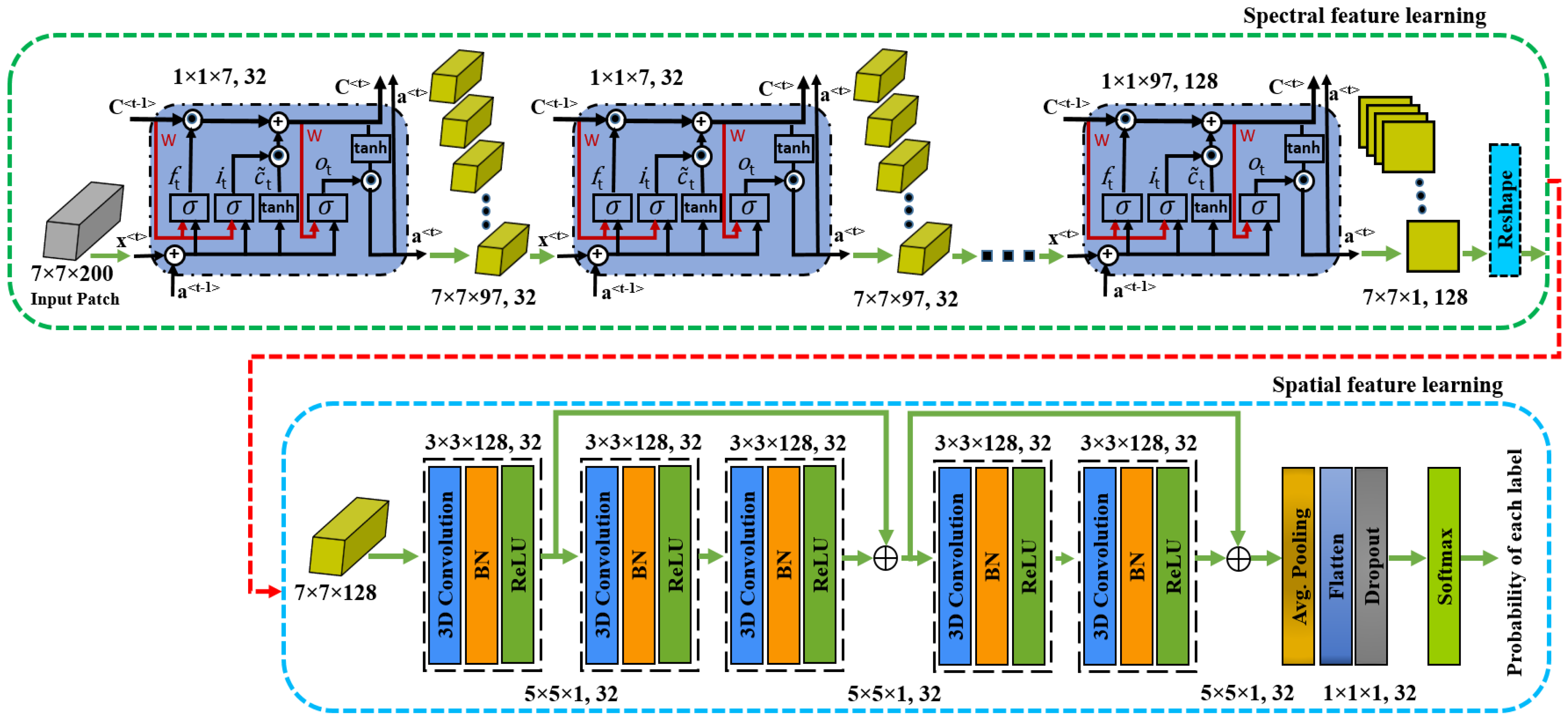
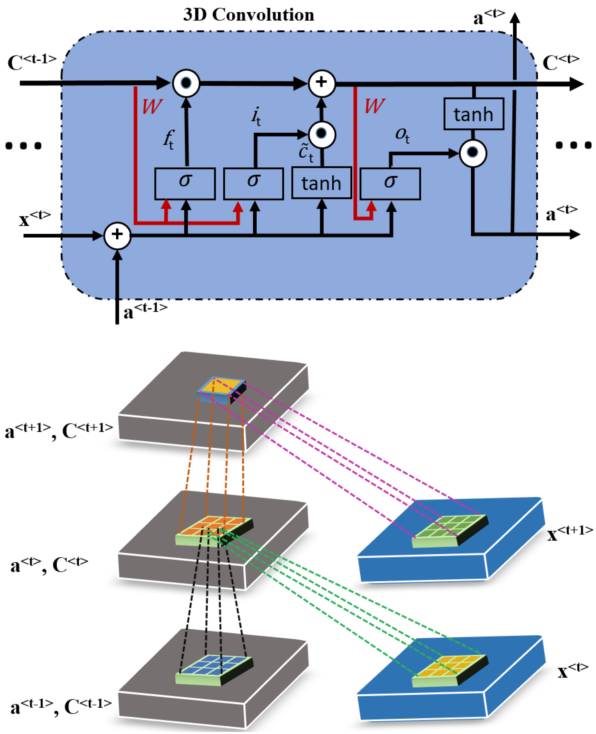
- The proposed framework SSCRN can learn both spatial and spectral feature representations jointly, without using any dimensionality reduction technique. The 3D ConvLSTM is exploited to learn the robust spectral feature representations, and the 3D CNN residual network is used to learn spatial features from HSI. This combination yields excellent performance.
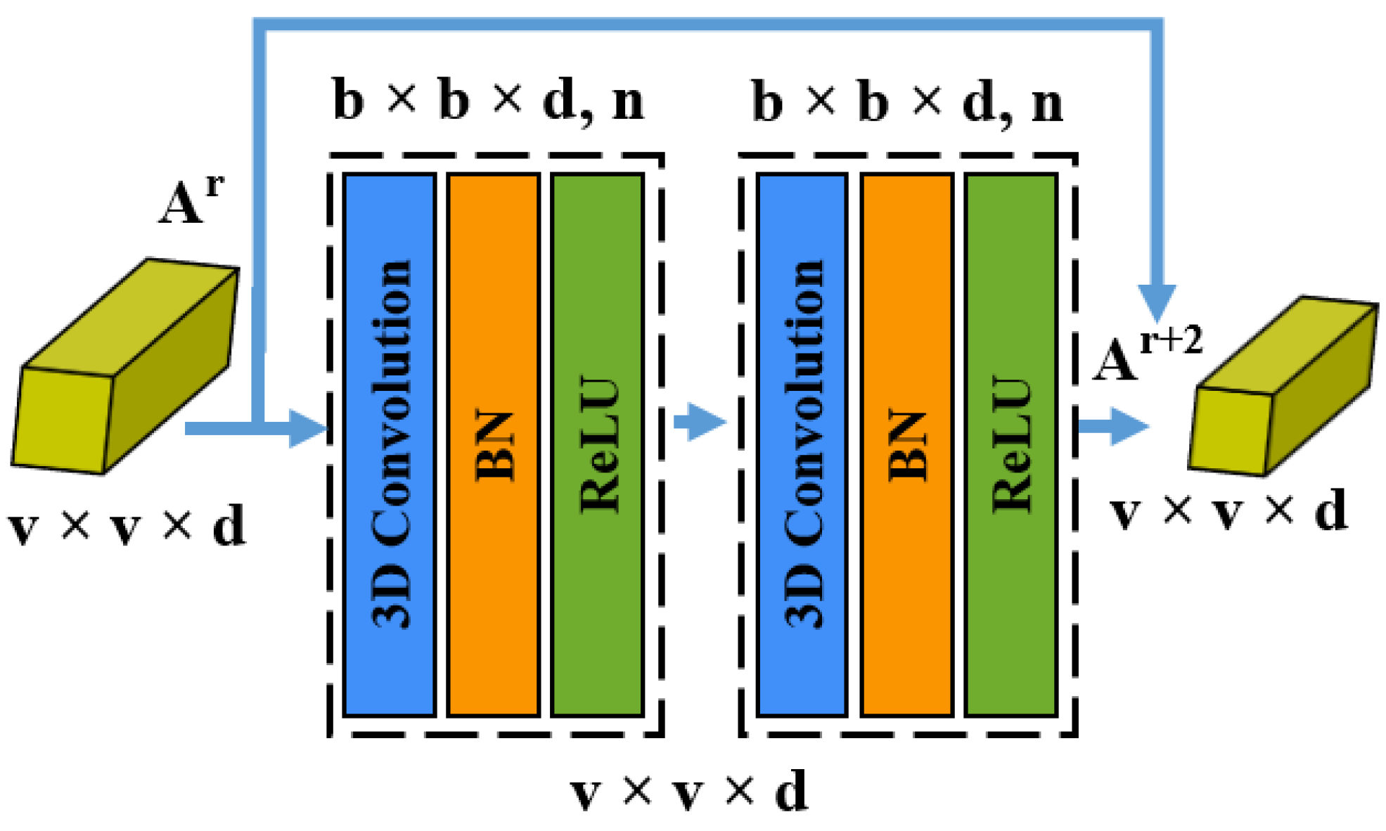
- To the best of the authors’ knowledge, this is the first time that 3D ConvLSTM and 3D CNN networks with skip connections are combined to build an end-to-end framework for HSI classification. This framework adopts residual connections to accelerate the training, mitigate the decreasing accuracy phenomenon, and improve the classification accuracy.
- The performance of the proposed framework is evaluated on three challenging benchmark datasets. The results confirm that SSCRN outperforms existing methods with limited labeled training samples.
2. Background
2.1. CNN
2.2. LSTM
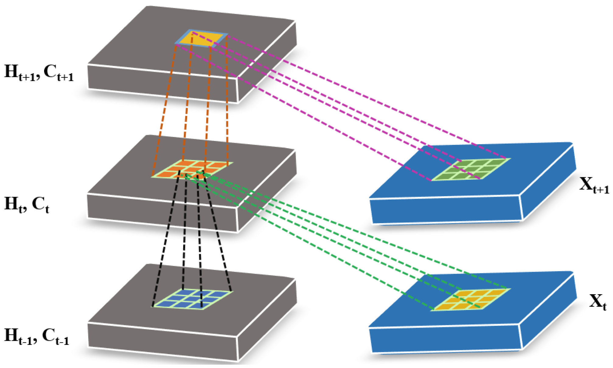
2.3. ConvLSTM
3. Proposed Methodology
3.1. 3D ConvLSTM Spectral Module
3.2. Deformable Process
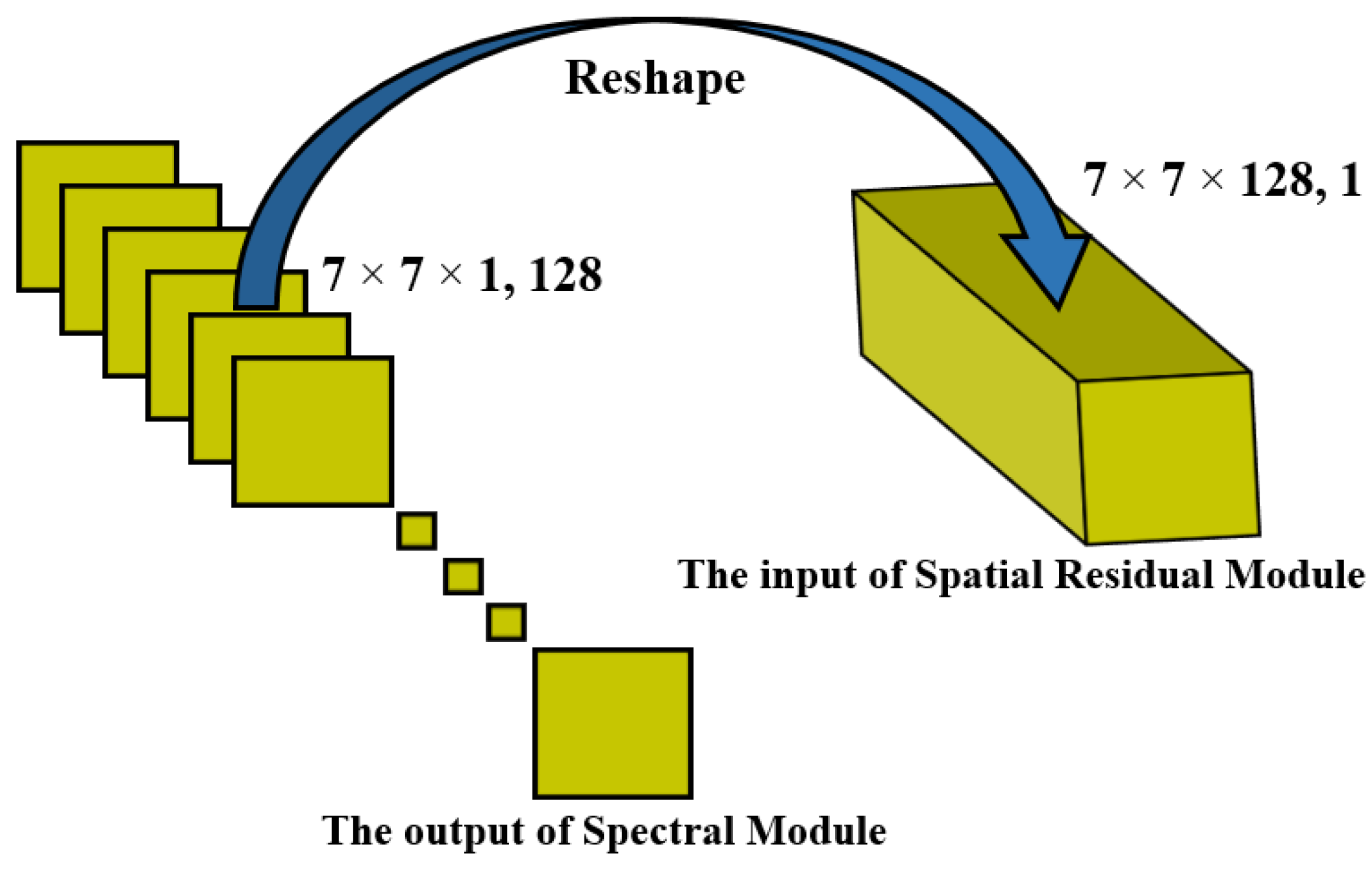
3.3. Three-Dimensional CNN Spatial Residual Module
4. Experimentations and Results Analysis
4.1. Experimental Data Sets
4.2. Experimental Settings
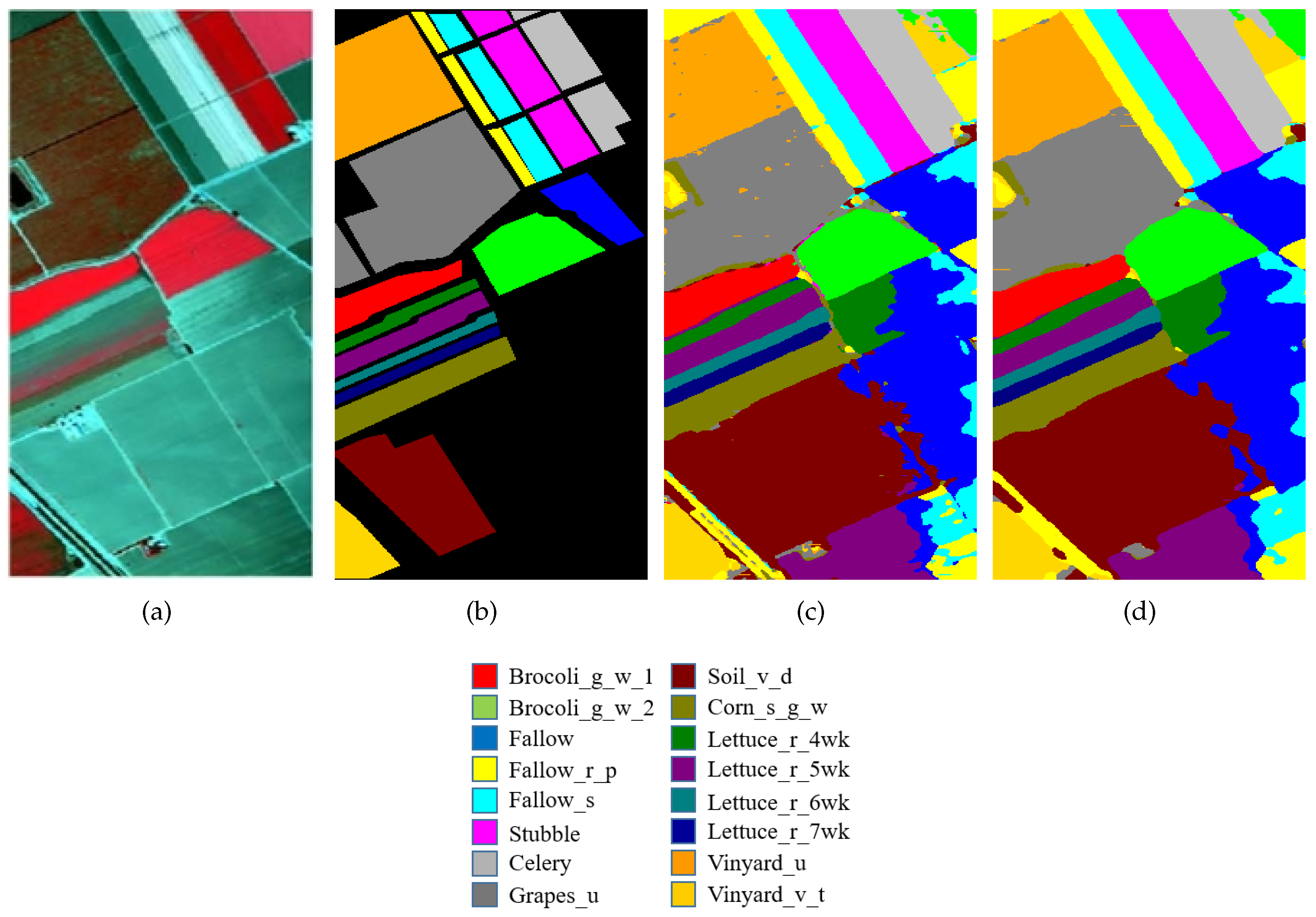
4.3. Classification Results
4.4. Impact of Training Ratio
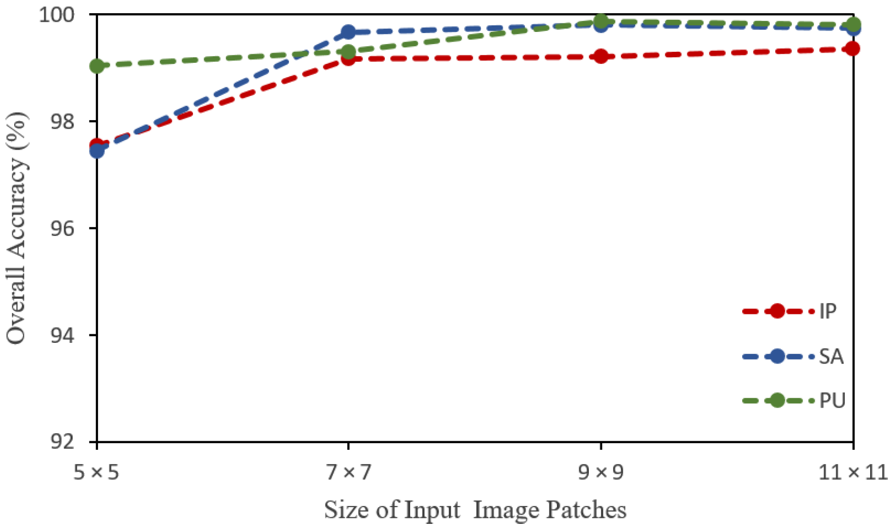
4.5. Impact of Spatial Size of the Input Image Patches
4.6. Impact of the Number of Convolution Kernels
4.7. Ablation Study
5. Discussion
6. Conclusions
Author Contributions
Funding
Data Availability Statement
Conflicts of Interest
References
- Khan, M.J.; Khan, H.S.; Yousaf, A.; Khurshid, K.; Abbas, A. Modern trends in hyperspectral image analysis: A review. IEEE Access 2018, 6, 14118–14129. [Google Scholar] [CrossRef]
- Wang, Q.; Yuan, Z.; Du, Q.; Li, X. GETNET: A general end-to-end 2-D CNN framework for hyperspectral image change detection. IEEE Trans. Geosci. Remote Sens. 2018, 57, 3–13. [Google Scholar] [CrossRef] [Green Version]
- Sun, H.; Zheng, X.; Lu, X.; Wu, S. Spectral-Spatial Attention Network for Hyperspectral Image Classification. IEEE Trans. Geosci. Remote Sens. 2019, 58, 3232–3245. [Google Scholar] [CrossRef]
- Maes, W.H.; Steppe, K. Perspectives for remote sensing with unmanned aerial vehicles in precision agriculture. Trends Plant Sci. 2019, 24, 152–164. [Google Scholar] [CrossRef] [PubMed]
- Tan, Y.; Lu, L.; Bruzzone, L.; Guan, R.; Chang, Z.; Yang, C. Hyperspectral Band Selection for Lithologic Discrimination and Geological Mapping. IEEE J. Sel. Top. Appl. Earth Obs. Remote Sens. 2020, 13, 471–486. [Google Scholar] [CrossRef]
- Yousefi, B.; Castanedo, C.I.; Bédard, É.; Beaudoin, G.; Maldague, X.P. Mineral identification in LWIR hyperspectral imagery applying sparse-based clustering. Quant. Infrared Thermogr. J. 2019, 16, 147–162. [Google Scholar] [CrossRef]
- Shimoni, M.; Haelterman, R.; Perneel, C. Hypersectral Imaging for Military and Security Applications: Combining Myriad Processing and Sensing Techniques. IEEE Geosci. Remote Sens. Mag. 2019, 7, 101–117. [Google Scholar] [CrossRef]
- Stuart, M.B.; McGonigle, A.J.; Willmott, J.R. Hyperspectral Imaging in Environmental Monitoring: A Review of Recent Developments and Technological Advances in Compact Field Deployable Systems. Sensors 2019, 19, 3071. [Google Scholar] [CrossRef] [PubMed] [Green Version]
- Wu, P.; Cui, Z.; Gan, Z.; Liu, F. Three-Dimensional ResNeXt Network Using Feature Fusion and Label Smoothing for Hyperspectral Image Classification. Sensors 2020, 20, 1652. [Google Scholar] [CrossRef] [PubMed] [Green Version]
- Zou, L.; Zhu, X.; Wu, C.; Liu, Y.; Qu, L. Spectral–Spatial Exploration for Hyperspectral Image Classification via the Fusion of Fully Convolutional Networks. IEEE J. Sel. Top. Appl. Earth Obs. Remote Sens. 2020, 13, 659–674. [Google Scholar] [CrossRef]
- Gan, Y.; Luo, F.; Liu, J.; Lei, B.; Zhang, T.; Liu, K. Feature extraction based multi-structure manifold embedding for hyperspectral remote sensing image classification. IEEE Access 2017, 5, 25069–25080. [Google Scholar] [CrossRef]
- Fauvel, M.; Tarabalka, Y.; Benediktsson, J.A.; Chanussot, J.; Tilton, J.C. Advances in spectral-spatial classification of hyperspectral images. Proc. IEEE 2012, 101, 652–675. [Google Scholar] [CrossRef] [Green Version]
- Belgiu, M.; Drăguţ, L. Random forest in remote sensing: A review of applications and future directions. ISPRS J. Photogramm. Remote Sens. 2016, 114, 24–31. [Google Scholar] [CrossRef]
- Jia, S.; Hu, J.; Zhu, J.; Jia, X.; Li, Q. Three-dimensional local binary patterns for hyperspectral imagery classification. IEEE Trans. Geosci. Remote Sens. 2017, 55, 2399–2413. [Google Scholar] [CrossRef]
- Xu, Y.; Wu, Z.; Wei, Z. Markov random field with homogeneous areas priors for hyperspectral image classification. In Proceedings of the 2014 IEEE Geoscience and Remote Sensing Symposium, Quebec City, QC, Canada, 13–18 July 2014; pp. 3426–3429. [Google Scholar]
- Quesada-Barriuso, P.; Argüello, F.; Heras, D.B. Spectral–Spatial classification of hyperspectral images using wavelets and extended morphological profiles. IEEE J. Sel. Top. Appl. Earth Obs. Remote Sens. 2014, 7, 1177–1185. [Google Scholar] [CrossRef]
- He, L.; Chen, X. A three-dimensional filtering method for spectral-spatial hyperspectral image classification. In Proceedings of the 2016 IEEE International Geoscience and Remote Sensing Symposium (IGARSS), Beijing, China, 10–15 July 2016; pp. 2746–2748. [Google Scholar]
- Bau, T.C.; Sarkar, S.; Healey, G. Hyperspectral region classification using a three-dimensional Gabor filterbank. IEEE Trans. Geosci. Remote Sens. 2010, 48, 3457–3464. [Google Scholar] [CrossRef]
- Yin, J.; Li, S.; Zhu, H.; Luo, X. Hyperspectral image classification using CapsNet with well-initialized shallow layers. IEEE Geosci. Remote Sens. Lett. 2019, 16, 1095–1099. [Google Scholar] [CrossRef]
- Zhang, L.; Zhang, L.; Du, B. Deep learning for remote sensing data: A technical tutorial on the state of the art. IEEE Geosci. Remote Sens. Mag. 2016, 4, 22–40. [Google Scholar] [CrossRef]
- Ma, A.; Filippi, A.M.; Wang, Z.; Yin, Z. Hyperspectral image classification using similarity measurements-based deep recurrent neural networks. Remote Sens. 2019, 11, 194. [Google Scholar] [CrossRef] [Green Version]
- Zhang, M.; Li, W.; Du, Q.; Gao, L.; Zhang, B. Feature extraction for classification of hyperspectral and LiDAR data using patch-to-patch CNN. IEEE Trans. Cybern. 2018, 50, 100–111. [Google Scholar] [CrossRef] [PubMed]
- Mustaqeem; Kwon, S. 1D-CNN: Speech Emotion Recognition System Using a Stacked Network with Dilated CNN Features. CMC-Comput. Mater. Contin. 2021, 67, 4039–4059. [Google Scholar] [CrossRef]
- Sargano, A.B.; Wang, X.; Angelov, P.; Habib, Z. Human action recognition using transfer learning with deep representations. In Proceedings of the 2017 International joint conference on neural networks (IJCNN), Anchorage, AK, USA, 14–19 May 2017; pp. 463–469. [Google Scholar]
- Farooque, G.; Sargano, A.B.; Shafi, I.; Ali, W. Coin recognition with reduced feature set sift algorithm using neural network. In Proceedings of the 2016 International Conference on Frontiers of Information Technology (FIT), Islamabad, Pakistan, 19–21 December 2016; pp. 93–98. [Google Scholar]
- Ashraf, M.; Geng, G.; Wang, X.; Ahmad, F.; Abid, F. A Globally Regularized Joint Neural Architecture for Music Classification. IEEE Access 2020, 8, 220980–220989. [Google Scholar] [CrossRef]
- Chen, Y.; Lin, Z.; Zhao, X.; Wang, G.; Gu, Y. Deep learning-based classification of hyperspectral data. IEEE J. Sel. Top. Appl. Earth Obs. Remote Sens. 2014, 7, 2094–2107. [Google Scholar] [CrossRef]
- Chen, Y.; Zhao, X.; Jia, X. Spectral–spatial classification of hyperspectral data based on deep belief network. IEEE J. Sel. Top. Appl. Earth Obs. Remote Sens. 2015, 8, 2381–2392. [Google Scholar] [CrossRef]
- Mou, L.; Ghamisi, P.; Zhu, X.X. Deep recurrent neural networks for hyperspectral image classification. IEEE Trans. Geosci. Remote Sens. 2017, 55, 3639–3655. [Google Scholar] [CrossRef] [Green Version]
- Yang, J.; Zhao, Y.Q.; Chan, J.C.W. Learning and transferring deep joint spectral–spatial features for hyperspectral classification. IEEE Trans. Geosci. Remote Sens. 2017, 55, 4729–4742. [Google Scholar] [CrossRef]
- Lee, H.; Kwon, H. Going deeper with contextual CNN for hyperspectral image classification. IEEE Trans. Image Process. 2017, 26, 4843–4855. [Google Scholar] [CrossRef] [PubMed] [Green Version]
- Zhao, W.; Du, S. Spectral–spatial feature extraction for hyperspectral image classification: A dimension reduction and deep learning approach. IEEE Trans. Geosci. Remote Sens. 2016, 54, 4544–4554. [Google Scholar] [CrossRef]
- Liu, B.; Yu, X.; Zhang, P.; Yu, A.; Fu, Q.; Wei, X. Supervised deep feature extraction for hyperspectral image classification. IEEE Trans. Geosci. Remote Sens. 2017, 56, 1909–1921. [Google Scholar] [CrossRef]
- Feng, F.; Wang, S.; Wang, C.; Zhang, J. Learning Deep Hierarchical Spatial–Spectral Features for Hyperspectral Image Classification Based on Residual 3D-2D CNN. Sensors 2019, 19, 5276. [Google Scholar] [CrossRef] [PubMed] [Green Version]
- Jia, S.; Zhao, B.; Tang, L.; Feng, F.; Wang, W. Spectral–spatial classification of hyperspectral remote sensing image based on capsule network. J. Eng. 2019, 2019, 7352–7355. [Google Scholar] [CrossRef]
- Li, X.; Ding, M.; Pižurica, A. Deep Feature Fusion via Two-Stream Convolutional Neural Network for Hyperspectral Image Classification. IEEE Trans. Geosci. Remote Sens. 2019, 58, 2615–2629. [Google Scholar] [CrossRef] [Green Version]
- Chen, Y.; Jiang, H.; Li, C.; Jia, X.; Ghamisi, P. Deep feature extraction and classification of hyperspectral images based on convolutional neural networks. IEEE Trans. Geosci. Remote Sens. 2016, 54, 6232–6251. [Google Scholar] [CrossRef] [Green Version]
- Li, Y.; Zhang, H.; Shen, Q. Spectral–spatial classification of hyperspectral imagery with 3D convolutional neural network. Remote Sens. 2017, 9, 67. [Google Scholar] [CrossRef] [Green Version]
- Zhong, Z.; Li, J.; Luo, Z.; Chapman, M. Spectral–spatial residual network for hyperspectral image classification: A 3-D deep learning framework. IEEE Trans. Geosci. Remote Sens. 2017, 56, 847–858. [Google Scholar] [CrossRef]
- Song, W.; Li, S.; Fang, L.; Lu, T. Hyperspectral image classification with deep feature fusion network. IEEE Trans. Geosci. Remote Sens. 2018, 56, 3173–3184. [Google Scholar] [CrossRef]
- Zhang, C.; Li, G.; Du, S.; Tan, W.; Gao, F. Three-dimensional densely connected convolutional network for hyperspectral remote sensing image classification. J. Appl. Remote Sens. 2019, 13, 016519. [Google Scholar] [CrossRef]
- Liu, Q.; Xiao, L.; Yang, J.; Chan, J.C.W. Content-guided convolutional neural network for hyperspectral image classification. IEEE Trans. Geosci. Remote Sens. 2020, 58, 6124–6137. [Google Scholar] [CrossRef]
- Liu, Q.; Xiao, L.; Yang, J.; Wei, Z. CNN-enhanced graph convolutional network with pixel-and superpixel-level feature fusion for hyperspectral image classification. IEEE Trans. Geosci. Remote Sens. 2020, 59, 8657–8671. [Google Scholar] [CrossRef]
- Fang, B.; Li, Y.; Zhang, H.; Chan, J.C.W. Hyperspectral images classification based on dense convolutional networks with spectral-wise attention mechanism. Remote Sens. 2019, 11, 159. [Google Scholar] [CrossRef] [Green Version]
- Xu, Q.; Xiao, Y.; Wang, D.; Luo, B. CSA-MSO3DCNN: Multiscale Octave 3D CNN with Channel and Spatial Attention for Hyperspectral Image Classification. Remote Sens. 2020, 12, 188. [Google Scholar] [CrossRef] [Green Version]
- Jamshidpour, N.; Aria, E.H.; Safari, A.; Homayouni, S. Adaptive Self-Learned Active Learning Framework for Hyperspectral Classification. In Proceedings of the 10th Workshop on Hyperspectral Imaging and Signal Processing: Evolution in Remote Sensing (WHISPERS), Amsterdam, The Netherlands, 24–26 September 2019; pp. 1–5. [Google Scholar]
- He, K.; Zhang, X.; Ren, S.; Sun, J. Deep residual learning for image recognition. In Proceedings of the IEEE Conference on Computer Vision and Pattern Recognition, Las Vegas, NV, USA, 27–30 June 2016; pp. 770–778. [Google Scholar]
- Ienco, D.; Gaetano, R.; Dupaquier, C.; Maurel, P. Land cover classification via multitemporal spatial data by deep recurrent neural networks. IEEE Geosci. Remote Sens. Lett. 2017, 14, 1685–1689. [Google Scholar] [CrossRef] [Green Version]
- Zhou, F.; Hang, R.; Liu, Q.; Yuan, X. Hyperspectral image classification using spectral-spatial LSTMs. Neurocomputing 2019, 328, 39–47. [Google Scholar] [CrossRef]
- Kwon, S. CLSTM: Deep feature-based speech emotion recognition using the hierarchical ConvLSTM network. Mathematics 2020, 8, 2133. [Google Scholar]
- Xingjian, S.; Chen, Z.; Wang, H.; Yeung, D.Y.; Wong, W.K.; Woo, W.C. Convolutional LSTM network: A machine learning approach for precipitation nowcasting. In Proceedings of the Advances in Neural Information Processing Systems, Montreal, QC, Canada, 7–12 December 2015; pp. 802–810. [Google Scholar]
- Liu, Q.; Zhou, F.; Hang, R.; Yuan, X. Bidirectional-convolutional LSTM based spectral-spatial feature learning for hyperspectral image classification. Remote Sens. 2017, 9, 1330. [Google Scholar] [CrossRef] [Green Version]
- Hu, W.S.; Li, H.C.; Pan, L.; Li, W.; Tao, R.; Du, Q. Feature extraction and classification based on spatial-spectral convlstm neural network for hyperspectral images. arXiv 2019, arXiv:1905.03577. [Google Scholar]
- Bioucas-Dias, J.M.; Plaza, A.; Camps-Valls, G.; Scheunders, P.; Nasrabadi, N.; Chanussot, J. Hyperspectral remote sensing data analysis and future challenges. IEEE Geosci. Remote Sens. Mag. 2013, 1, 6–36. [Google Scholar] [CrossRef] [Green Version]
- Liu, S.; Marinelli, D.; Bruzzone, L.; Bovolo, F. A review of change detection in multitemporal hyperspectral images: Current techniques, applications, and challenges. IEEE Geosci. Remote Sens. Mag. 2019, 7, 140–158. [Google Scholar] [CrossRef]
- Hochreiter, S.; Schmidhuber, J. Long short-term memory. Neural Comput. 1997, 9, 1735–1780. [Google Scholar] [CrossRef]
- Mei, X.; Pan, E.; Ma, Y.; Dai, X.; Huang, J.; Fan, F.; Du, Q.; Zheng, H.; Ma, J. Spectral-spatial attention networks for hyperspectral image classification. Remote Sens. 2019, 11, 963. [Google Scholar] [CrossRef] [Green Version]
- Hu, W.S.; Li, H.C.; Pan, L.; Li, W.; Tao, R.; Du, Q. Spatial–spectral feature extraction via deep ConvLSTM neural networks for hyperspectral image classification. IEEE Trans. Geosci. Remote Sens. 2020, 58, 4237–4250. [Google Scholar] [CrossRef]
- Kingma, D.P.; Ba, J. Adam: A method for stochastic optimization. arXiv 2014, arXiv:1412.6980. [Google Scholar]
- Seifi Majdar, R.; Ghassemian, H. A probabilistic SVM approach for hyperspectral image classification using spectral and texture features. Int. J. Remote Sens. 2017, 38, 4265–4284. [Google Scholar] [CrossRef]
- Plaza, J.; Plaza, A.J.; Barra, C. Multi-channel morphological profiles for classification of hyperspectral images using support vector machines. Sensors 2009, 9, 196–218. [Google Scholar] [CrossRef] [PubMed] [Green Version]
- Santara, A.; Mani, K.; Hatwar, P.; Singh, A.; Garg, A.; Padia, K.; Mitra, P. BASS net: Band-adaptive spectral-spatial feature learning neural network for hyperspectral image classification. IEEE Trans. Geosci. Remote Sens. 2017, 55, 5293–5301. [Google Scholar] [CrossRef] [Green Version]
- Yu, C.; Han, R.; Song, M.; Liu, C.; Chang, C.I. A simplified 2D-3D CNN architecture for hyperspectral image classification based on spatial–spectral fusion. IEEE J. Sel. Top. Appl. Earth Obs. Remote Sens. 2020, 13, 2485–2501. [Google Scholar] [CrossRef]
- Sellami, A.; Farah, M.; Farah, I.R.; Solaiman, B. Hyperspectral imagery classification based on semi-supervised 3-D deep neural network and adaptive band selection. Expert Syst. Appl. 2019, 129, 246–259. [Google Scholar] [CrossRef]
- Zhao, G.; Liu, G.; Fang, L.; Tu, B.; Ghamisi, P. Multiple convolutional layers fusion framework for hyperspectral image classification. Neurocomputing 2019, 339, 149–160. [Google Scholar] [CrossRef]
- Guo, H.; Liu, J.; Xiao, Z.; Xiao, L. Deep CNN-based hyperspectral image classification using discriminative multiple spatial-spectral feature fusion. Remote Sens. Lett. 2020, 11, 827–836. [Google Scholar] [CrossRef]
- Qu, L.; Zhu, X.; Zheng, J.; Zou, L. Triple-Attention-Based Parallel Network for Hyperspectral Image Classification. Remote Sens. 2021, 13, 324. [Google Scholar] [CrossRef]


| No. | Class Name | Train | Validation | Test | Total |
|---|---|---|---|---|---|
| 1 | Alfalfa | 5 | 5 | 36 | 46 |
| 2 | Corn-n | 143 | 143 | 1142 | 1428 |
| 3 | Corn-m | 83 | 83 | 664 | 830 |
| 4 | Corn | 24 | 24 | 189 | 237 |
| 5 | Grass-p | 49 | 49 | 385 | 483 |
| 6 | Grass-t | 73 | 73 | 584 | 730 |
| 7 | Grass-p-m | 3 | 3 | 22 | 28 |
| 8 | Hay-w | 48 | 48 | 382 | 478 |
| 9 | Oats | 2 | 2 | 16 | 20 |
| 10 | Soybean-n | 98 | 98 | 776 | 972 |
| 11 | Soybean-m | 246 | 246 | 1963 | 2455 |
| 12 | Soybean-c | 60 | 60 | 473 | 593 |
| 13 | Wheat | 21 | 21 | 163 | 205 |
| 14 | Woods | 127 | 127 | 1011 | 1265 |
| 15 | Buildings-g-t-d | 39 | 39 | 308 | 386 |
| 16 | Stone-s-t | 10 | 10 | 73 | 93 |
| Total | 1031 | 1031 | 8187 | 10,249 |
| No. | Class Name | Train | Validation | Test | Total |
|---|---|---|---|---|---|
| 1 | Brocoli_g_w_1 | 101 | 101 | 1807 | 2009 |
| 2 | Brocoli_g_w_2 | 187 | 187 | 3352 | 3726 |
| 3 | Fallow | 99 | 99 | 1778 | 1976 |
| 4 | Fallow_r_p | 70 | 70 | 1254 | 1394 |
| 5 | Fallow_s | 134 | 134 | 2410 | 2678 |
| 6 | Stubble | 198 | 198 | 3563 | 3959 |
| 7 | Celery | 179 | 179 | 3221 | 3579 |
| 8 | Grapes_u | 564 | 564 | 10,143 | 11,271 |
| 9 | Soil_v_d | 311 | 311 | 5581 | 6203 |
| 10 | Corn_s_g_w | 164 | 164 | 2950 | 3278 |
| 11 | Lettuce_r_4wk | 54 | 54 | 960 | 1068 |
| 12 | Lettuce_r_5wk | 97 | 97 | 1733 | 1927 |
| 13 | Lettuce_r_6wk | 46 | 46 | 824 | 916 |
| 14 | Lettuce_r_7wk | 54 | 54 | 962 | 1070 |
| 15 | Vinyard_u | 364 | 364 | 6540 | 7268 |
| 16 | Vinyard_v_t | 91 | 91 | 1625 | 1807 |
| Total | 2713 | 2713 | 48,703 | 54,129 |
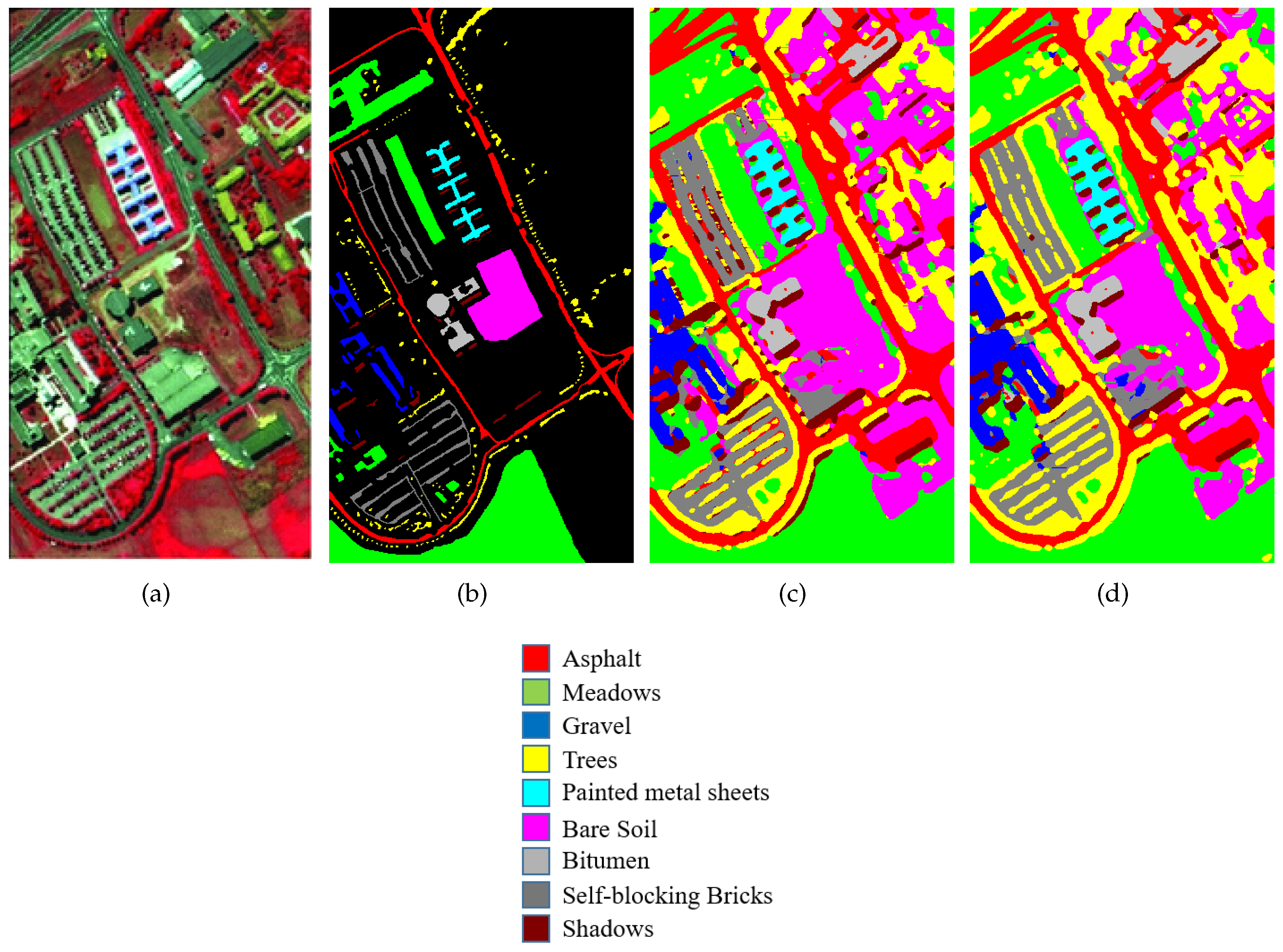
| No. | Class Name | Train | Validation | Test | Total |
|---|---|---|---|---|---|
| 1 | Asphalt | 332 | 332 | 5967 | 6631 |
| 2 | Meadows | 933 | 933 | 16,783 | 18,649 |
| 3 | Gravel | 105 | 105 | 1889 | 2099 |
| 4 | Trees | 154 | 154 | 2756 | 3064 |
| 5 | Painted metal sheets | 68 | 68 | 1209 | 1345 |
| 6 | Bare Soil | 252 | 252 | 4525 | 5029 |
| 7 | Bitumen | 67 | 67 | 1196 | 1330 |
| 8 | Self-blocking Bricks | 185 | 185 | 3312 | 3682 |
| 9 | Shadows | 48 | 48 | 851 | 947 |
| Total | 2144 | 2144 | 38,488 | 42,776 |
| Datasets | Dropout | BN | Dropout & BN |
|---|---|---|---|
| IP | 96.90 | 98.69 | 99.17 |
| SA | 98.42 | 99.15 | 99.67 |
| PU | 97.97 | 98.81 | 99.31 |
| Layer Name | Output Shape | Kernel Size | No. of Convolutional Kernel | Stride | Padding |
|---|---|---|---|---|---|
| ConvLSTM3D | 7 × 7 × 97 × 32 | 1 × 1 × 7 | 32 | 1 × 1 × 2 | Valid |
| ConvLSTM3D | 7 × 7 × 97 × 32 | 1 × 1 × 7 | 32 | 1 × 1 × 1 | Same |
| ConvLSTM3D | 7 × 7 × 97 × 32 | 1 × 1 × 7 | 32 | 1 × 1 × 1 | Same |
| ConvLSTM3D | 7 × 7 × 1 × 128 | 1 × 1 × 97 | 128 | 1 × 1 × 1 | N/A |
| Reshape | 7 × 7 × 128 × 1 | N/A | N/A | N/A | N/A |
| Conv3D | 5 × 5 × 1 × 32 | 3 × 3 × 128 | 32 | 1 × 1 × 1 | N/A |
| Conv3D | 5 × 5 × 1 × 32 | 3 × 3 × 128 | 32 | 1 × 1 × 1 | Same |
| Conv3D | 5 × 5 × 1 × 32 | 3 × 3 × 128 | 32 | 1 × 1 × 1 | Same |
| Skip connection | |||||
| Conv3D | 5 × 5 × 1 × 32 | 3 × 3 × 128 | 32 | 1 × 1 × 1 | Same |
| Conv3D | 5 × 5 × 1 × 32 | 3 × 3 × 128 | 32 | 1 × 1 × 1 | Same |
| Skip connection | |||||
| AveragePooling3D | 1 × 1 × 1 × 32 | N/A | N/A | 1 × 1 × 1 | N/A |
| Flatten | 32 | N/A | N/A | N/A | N/A |
| Dropout | 32 | 0.25 | N/A | N/A | N/A |
| Dense (Output) | N | N/A | N/A | N/A | N/A |
| Hyper-Parameter | 3D-CNN | BASSNet | 2D-3D CNN | SS3FC | ADR | FFDN-SY | TAP-Net | SSCRN |
|---|---|---|---|---|---|---|---|---|
| optimizer | SGD | Adam | RMSprop | Adam | - | Adam | Adam | Adam |
| Learning-rate | 0.001, 0.0001 | 0.0005 | 0.001 | 0.01 | 0.0005, 0.001 | 0.01 | 0.01 | 0.0003, 0.0001 |
| Batch size | 10 | 100 | 100 | - | - | 200 | 32 | 32, 64 |
| Dropout | 0.5 | 0.5 | 0.3, 0.8 | - | - | - | - | 0.25 |
| Activation | ReLU | ReLU | ReLU | ReLU | ReLU | ReLU | ReLU | tanh, ReLU |
| Iterations | 100K | 1000 | 5000 | 40-80 | 150–300 | 9000 | - | 300 |
| Loss-function | - | Cross-entropy | - | Focal loss | softmax | - | Focal loss | Categorical cross-entropy |
| Class | SVM | 3D-CNN | BASSNet | 2D–3D CNN | SS3FC | ADR | FCLFN | FFDN-SY | TAP-Net | SSCRN |
|---|---|---|---|---|---|---|---|---|---|---|
| 1 | - | - | - | 100.0 | 40.40 | 97.96 | 95.12 | - | 70.98 | 100.0 |
| 2 | 72.17 | 90.10 | 96.09 | 98.36 | 77.89 | 97.21 | 99.38 | 95.09 | 76.54 | 98.17 |
| 3 | 67.11 | 97.10 | 98.25 | 97.80 | 60.74 | 97.47 | 100.0 | 98.98 | 75.62 | 99.40 |
| 4 | - | - | - | 97.20 | 11.80 | 99.53 | 100.0 | - | 46.83 | 100.0 |
| 5 | 91.07 | 100.0 | 100.0 | 99.30 | 67.50 | 98.88 | 95.16 | 99.56 | 69.78 | 98.00 |
| 6 | 94.14 | - | 99.24 | 99.07 | 91.95 | 98.51 | 99.24 | 99.67 | 94.77 | 99.50 |
| 7 | - | - | - | 100.0 | 20.14 | 95.24 | 72.10 | - | 80.40 | 100.0 |
| 8 | 98.64 | 100.0 | 100.0 | 99.83 | 81.71 | 97.73 | 99.53 | 99.89 | 98.95 | 100.0 |
| 9 | - | - | - | 92.72 | 31.67 | 94.44 | 88.89 | - | 70.03 | 100.0 |
| 10 | 73.65 | 95.90 | 94.82 | 97.34 | 78.15 | 97.24 | 99.54 | 97.98 | 84.59 | 98.43 |
| 11 | 86.23 | 87.10 | 94.41 | 98.23 | 69.32 | 97.70 | 98.64 | 94.20 | 80.39 | 99.53 |
| 12 | 59.43 | 96.40 | 97.46 | 97.66 | 40.81 | 97.83 | 92.68 | 99.53 | 76.84 | 99.58 |
| 13 | - | - | - | 99.32 | 93.43 | 95.81 | 100.0 | - | 97.13 | 100.0 |
| 14 | 97.69 | 99.40 | 99.90 | 99.01 | 91.77 | 99.83 | 99.91 | 99.25 | 94.83 | 99.50 |
| 15 | - | - | - | 98.60 | 37.93 | 96.49 | 97.41 | - | 51.70 | 99.34 |
| 16 | - | - | - | 92.59 | 75.19 | 96.47 | 97.59 | - | 92.27 | 97.29 |
| OA | 82.58 | 93.61 | 96.77 | 98.33 | 71.47 | 97.89 | 98.56 | 96.96 | 81.35 | 99.17 |
| AA | 82.46 | / | / | / | 60.65 | 97.39 | 95.94 | 98.24 | 78.85 | 99.29 |
| k | 79.42 | / | / | / | / | 98.72 | 98.36 | 96.36 | 0.787 | 99.05 |
| Class | SVM | 3D-CNN | BASSNet | 2D–3D CNN | SS3FC | ADR | FCLFN | FFDN-SY | TAP-Net | SSCRN |
|---|---|---|---|---|---|---|---|---|---|---|
| 1 | 82.64 | 100.0 | 100.0 | 99.81 | 92.36 | 96.73 | 98.54 | 99.96 | 98.73 | 99.94 |
| 2 | 86.31 | 100.0 | 99.97 | 99.65 | 92.58 | 98.50 | 99.97 | 99.96 | 99.71 | 100.0 |
| 3 | 98.15 | 100.0 | 100.0 | 99.75 | 66.35 | 96.06 | 95.71 | 99.61 | 91.29 | 100.0 |
| 4 | 96.51 | 99.30 | 99.66 | 99.37 | 98.13 | 98.80 | 95.51 | 99.88 | 98.78 | 98.88 |
| 5 | 97.63 | 98.50 | 99.59 | 98.68 | 95.63 | 97.88 | 95.06 | 99.80 | 96.27 | 100.0 |
| 6 | 98.96 | 100.0 | 100.0 | 99.99 | 99.30 | 98.87 | 99.97 | 99.77 | 99.26 | 100.0 |
| 7 | 98.03 | 99.80 | 99.91 | 99.88 | 99.43 | 96.58 | 99.97 | 99.80 | 99.35 | 100.0 |
| 8 | 95.34 | 83.40 | 90.11 | 98.05 | 69.27 | 98.61 | 99.71 | 93.77 | 84.76 | 99.42 |
| 9 | 90.45 | 99.60 | 99.73 | 99.80 | 99.67 | 98.92 | 100.0 | 99.75 | 98.13 | 99.92 |
| 10 | 82.54 | 94.60 | 97.46 | 99.86 | 84.07 | 98.30 | 99.66 | 99.43 | 88.56 | 99.69 |
| 11 | 83.21 | 99.30 | 99.08 | 98.67 | 85.31 | 98.96 | 94.80 | 99.98 | 84.59 | 99.36 |
| 12 | 82.14 | 100.0 | 100.0 | 99.92 | 97.98 | 99.71 | 99.53 | 99.95 | 99.02 | 99.88 |
| 13 | 84.56 | 100.0 | 99.44 | 99.89 | 98.45 | 98.78 | 98.79 | 99.85 | 98.07 | 100.0 |
| 14 | 86.57 | 100.0 | 100.0 | 99.40 | 87.32 | 98.96 | 95.28 | 99.90 | 94.59 | 99.16 |
| 15 | 92.93 | 100.0 | 83.94 | 97.76 | 52.31 | 98.01 | 98.08 | 96.63 | 69.09 | 99.17 |
| 16 | - | 98.00 | 99.38 | 99.88 | 59.97 | 98.77 | 99.16 | 99.86 | 90.71 | 100.0 |
| OA | 94.82 | 95.07 | 95.36 | 99.07 | 81.32 | 98.29 | 98.59 | 98.04 | 90.31 | 99.67 |
| AA | / | / | / | / | 86.13 | 98.28 | 98.11 | 99.24 | 93.18 | 99.71 |
| k | / | / | / | / | / | 98.16 | 98.69 | 97.81 | 0.881 | 99.64 |
| Class | SVM | 3D-CNN | BASSNet | 2D–3D CNN | SS3FC | ADR | FCLFN | FFDN-SY | TAP-Net | SSCRN |
|---|---|---|---|---|---|---|---|---|---|---|
| 1 | 93.84 | 94.60 | 97.71 | 99.42 | 97.48 | 98.01 | 97.03 | 98.24 | 95.67 | 99.88 |
| 2 | 95.88 | 96.00 | 97.93 | 99.93 | 90.86 | 98.20 | 100 | 98.90 | 97.61 | 99.92 |
| 3 | 72.80 | 95.50 | 94.95 | 98.69 | 58.75 | 98.15 | 95.14 | 98.07 | 73.08 | 98.71 |
| 4 | 88.23 | 95.90 | 97.80 | 99.88 | 84.81 | 99.23 | 88.49 | 97.82 | 94.23 | 99.52 |
| 5 | 98.05 | 100.0 | 100.0 | 99.97 | 94.82 | 99.31 | 99.18 | 99.93 | 99.48 | 100.0 |
| 6 | 84.51 | 94.10 | 96.60 | 99.45 | 23.59 | 99.41 | 99.46 | 99.46 | 84.17 | 96.58 |
| 7 | 82.70 | 97.50 | 98.14 | 99.47 | 61.61 | 98.92 | 95.89 | 99.79 | 59.92 | 100.0 |
| 8 | 88.37 | 88.80 | 95.46 | 97.89 | 88.84 | 98.08 | 100.0 | 98.52 | 83.60 | 98.61 |
| 9 | 99.56 | 99.50 | 100.0 | 99.96 | 88.68 | 98.06 | 96.20 | 99.69 | 99.33 | 100.0 |
| OA | 91.64 | 95.97 | 97.48 | 99.54 | 79.89 | 98.45 | 98.17 | 98.78 | 91.64 | 99.31 |
| AA | 89.33 | / | / | / | 76.60 | 98.60 | 96.80 | 98.93 | 87.45 | 99.24 |
| k | 88.88 | / | / | / | / | 98.53 | 97.58 | 98.36 | 0.892 | 99.09 |
| Spatial Input Size | IP (OA) | IP (AA) | IP (k) | SA (OA) | SA (AA) | SA (k) | PU (OA) | PU (AA) | PU (k) |
|---|---|---|---|---|---|---|---|---|---|
| 5 × 5 | 97.55 | 98.85 | 97.78 | 97.45 | 98.40 | 97.16 | 99.04 | 98.28 | 98.72 |
| 7 × 7 | 99.17 | 99.29 | 99.05 | 99.67 | 99.71 | 99.64 | 99.31 | 99.24 | 99.09 |
| 9 × 9 | 99.21 | 99.20 | 98.83 | 99.81 | 99.89 | 99.79 | 99.88 | 99.89 | 99.84 |
| 11 × 11 | 99.35 | 99.28 | 99.13 | 99.75 | 99.78 | 99.65 | 99.82 | 99.60 | 99.76 |
| Sequence | Dataset | OA | AA | k |
|---|---|---|---|---|
| IP | 99.17 | 99.29 | 99.05 | |
| Spectral–Spatial | SA | 99.67 | 99.71 | 99.64 |
| PU | 99.31 | 99.24 | 99.09 | |
| IP | 98.97 | 96.82 | 98.40 | |
| Spatial–Spectral | SA | 99.01 | 99.14 | 98.56 |
| PU | 99.06 | 99.03 | 98.37 |
Publisher’s Note: MDPI stays neutral with regard to jurisdictional claims in published maps and institutional affiliations. |
© 2021 by the authors. Licensee MDPI, Basel, Switzerland. This article is an open access article distributed under the terms and conditions of the Creative Commons Attribution (CC BY) license (https://creativecommons.org/licenses/by/4.0/).
Share and Cite
Farooque, G.; Xiao, L.; Yang, J.; Sargano, A.B. Hyperspectral Image Classification via a Novel Spectral–Spatial 3D ConvLSTM-CNN. Remote Sens. 2021, 13, 4348. https://doi.org/10.3390/rs13214348
Farooque G, Xiao L, Yang J, Sargano AB. Hyperspectral Image Classification via a Novel Spectral–Spatial 3D ConvLSTM-CNN. Remote Sensing. 2021; 13(21):4348. https://doi.org/10.3390/rs13214348
Chicago/Turabian StyleFarooque, Ghulam, Liang Xiao, Jingxiang Yang, and Allah Bux Sargano. 2021. "Hyperspectral Image Classification via a Novel Spectral–Spatial 3D ConvLSTM-CNN" Remote Sensing 13, no. 21: 4348. https://doi.org/10.3390/rs13214348
APA StyleFarooque, G., Xiao, L., Yang, J., & Sargano, A. B. (2021). Hyperspectral Image Classification via a Novel Spectral–Spatial 3D ConvLSTM-CNN. Remote Sensing, 13(21), 4348. https://doi.org/10.3390/rs13214348