Abstract
In recent years, deep learning-based models have produced encouraging results for hyperspectral image (HSI) classification. Specifically, Convolutional Long Short-Term Memory (ConvLSTM) has shown good performance for learning valuable features and modeling long-term dependencies in spectral data. However, it is less effective for learning spatial features, which is an integral part of hyperspectral images. Alternatively, convolutional neural networks (CNNs) can learn spatial features, but they possess limitations in handling long-term dependencies due to the local feature extraction in these networks. Considering these factors, this paper proposes an end-to-end Spectral-Spatial 3D ConvLSTM-CNN based Residual Network (SSCRN), which combines 3D ConvLSTM and 3D CNN for handling both spectral and spatial information, respectively. The contribution of the proposed network is twofold. Firstly, it addresses the long-term dependencies of spectral dimension using 3D ConvLSTM to capture the information related to various ground materials effectively. Secondly, it learns the discriminative spatial features using 3D CNN by employing the concept of the residual blocks to accelerate the training process and alleviate the overfitting. In addition, SSCRN uses batch normalization and dropout to regularize the network for smooth learning. The proposed framework is evaluated on three benchmark datasets widely used by the research community. The results confirm that SSCRN outperforms state-of-the-art methods with an overall accuracy of 99.17%, 99.67%, and 99.31% over Indian Pines, Salinas, and Pavia University datasets, respectively. Moreover, it is worth mentioning that these excellent results were achieved with comparatively fewer epochs, which also confirms the fast learning capabilities of the SSCRN.
1. Introduction
It is now possible to acquire hyperspectral images (HSIs) with numerous contiguous spectral bands due to the advancement of imaging technology and hyperspectral sensors [1]. A hyperspectral image includes hundreds of small spectral bands with 2D spatial information of different land covers. The abundant spectral information enables HSIs to be successfully applied in various research fields, such as change detection [2], urban planning [3], precision agriculture [4], geology and mineral resources [5,6], national defense [7], and environment monitoring [8]. For these research domains, an important step is a robust and accurate image classification, which aims at identifying the unique category of each pixel. The HSI is a 3D data cube that combines spectral and spatial information, where the spatial resolution is shallow compared to the spectral resolution. It can only provide fewer details on the geometric relationship between image pixels. Therefore, spectral information is more important to identify the variety of ground materials accurately [9]. As an important research topic, HSI classification has received a great deal of attention, and several techniques have been proposed over the last few decades. However, due to the complex nature of HSIs and the scarcity of labeled samples, it remains a challenging task [10].
Early classification techniques were mainly based on two steps: traditional handcrafted feature engineering followed by generic trainable classifiers [9]. Firstly, the most representative features were obtained by utilizing handcrafted feature descriptors and reducing the dimensionality of HSI [11]. Secondly, the traditional machine learning classifiers were trained through a non-linear transformation using the extracted features [12]. Support vector machines (SVM) and random forest (RF) are typical examples of these classifiers [13]. In this direction, a number of spatial feature descriptors such as local binary patterns (LBP) [14], Markov random fields (MRFs) [15], extended morphological profile (EMP) [16], spatial filtering [17], and 3D Gabor features [18] were employed to achieve suitable feature representation. However, due to the separation of feature extraction and classification processes, the adaptability between features and classifiers was not optimal [19,20]. Moreover, these methods had a limited capability to represent spectral and spatial information together due to the curse of dimensionality [10]. Consequently, the need for more robust feature extraction and classification methods was prevalent for better performance.
In recent years, deep learning-based approaches have superseded the traditional handcrafted feature-based methods for HSI classification. They have attracted a great deal of attention for employing an end-to-end strategy for feature extraction and classification that reduces the chances of information loss during the pre-processing of of HSI and improves the classification results [10,21,22]. Beside HSI classification, CNN-based techniques have also been employed for several tasks such as speech emotion recognition [23], human activity recognition [24], coin recognition [25], and music classification [26]. Initial deep learning-based methods employed 1D networks such as stacked autoencoder (SAE) [27], deep belief networks (BDNs) [28], recurrent neural networks (RNNs) [29], and CNNs [30]. These methods achieved better accuracy than their predecessor handcrafted approaches; however, due to 1D input requirements, these models suffered from spatial information loss.
Consequently, several 2D CNN-based methods were introduced for HSI classification [31]. In contrast to the previous methods, image patches were considered as inputs, and a weight-sharing mechanism was introduced to acquire the spatial and spectral information for classification. Along these lines, a CNN model with three convolutions and one fully connected layer was proposed by Zhao et al. [32]. Due to its simpler structure, this model learned spatial features but could not use spectral information. Another deep feature extraction approach based on the Siamese CNN that included a margin ranking loss function to ensure high interclass variability and low intraclass variability was reported in [33]. One of the significant challenges in the CNN-based model is learning the spectral features and combining them with spatial features. In this direction, Lee et al. [31] presented a deep contextual CNN technique to predict the label of each pixel by utilizing local spectral–spatial features. The spectral and spatial features were extracted from multi-scale filters using 2D CNN and then merged to produce a combined spectral–spatial feature map. However, 2D CNN-based techniques cannot effectively use spectral and spatial information at the same time, and chances of information loss are high during the feature learning process [34]. Another method [35] proposed a hybrid architecture based on 1D and 2D CNN layers to learn spectral and spatial information, respectively.
To address the limitations of 2D CNN based networks, 3D CNN models were adopted to obtain spatial–spectral features directly from raw HSI [36]. In this direction, a 3D CNN model was proposed in [37], where 3D image patches were considered as input to learn the spatial–spectral information from HSI. Li et al. [38] proposed a variation to this model to obtain spectral–spatial features simultaneously using spatial filtering to take full benefit of structural properties of 3D HSI data. However, 3D CNN approaches have many parameters and quickly lead to overfitting, particularly when training samples are limited. Zhong et al. [39] developed spectral and spatial residual blocks to alleviate the declining accuracy due to overfitting and learned the discriminative features from spatial contexts and spectral signatures. As a variation to this method, Song et al. [40] introduced a deep feature fusion network based on residual learning to smooth the training of the deep model. Further, a densely connected 3D CNN (3D-DensNet) [41] was proposed to learn more robust spatial–spectral features. Lui et al. [42] introduced a content-guided CNN (CGCNN), which adaptively adjusts its kernel shape according to the spatial distribution of land covers. Another heterogeneous model based on CNN and graph convolutional network (GCN) was proposed in [43] to learn complementary spectral–spatial features at pixel and super-pixel levels. Other methods extended the 3D CNN by employing the concepts of attention mechanism [44], multi-scale convolution [45], and active learning [46] to improve classification accuracy. The major concern with the 3D CNN-based method is the degradation of accuracy due to very deep models as architectures become gradually complex with the growing number of hyper-parameters. Moreover, CNN-based models cannot handle long-term dependencies in spectral data [47].
Long Short-Term Memory (LSTM) [48] has proved its stability and strength in handling long-term dependencies in numerous computer vision tasks such as HSI classification [49] and speech emotion recognition [50]. Since HSIs are intensively sampled from the whole spectrum, dependencies between various spectral bands are expected. In this direction, Ienco et al. [48] proposed an LSTM-based model to perform classification tasks over multi-temporal satellite images. Further, Zhou et al. [49] introduced a spectral–spatial LSTMs (SSLSTMs) consisting of two independent LSTMs: spectral LSTM (SeLSTM) and spatial LSTM (SaLSTM). However, LSTM is limited in dealing with spectral–spatial and spatial–temporal data because it requires converting the input data into a 1D form, which causes a loss of essential spatial information. To overcome these limitations, Shi et al. [51] replaced the 1D data operation of each gate in LSTM with multi-dimensional processing and introduced convolutional LSTM (ConvLSTM). In ConvLSTM, 2D and 3D convolution filters can be used to construct the ConvLSTM2D and ConvLSTM3D, respectively. Motivated by this, Liu et al. [52] developed a model for obtaining spatial–spectral characteristics for HSI classification based on Bidirectional-Convolutional LSTM. Further, a spatial–spectral ConvLSTM2D neural network (SSCL2DNN) was introduced in [53] to manage the long-term dependencies and to obtain more discriminative features. Furthermore, ConvLSTM3D was used to simulate spatial and spectral information more efficiently.
Although deep learning-based approaches demonstrated encouraging performance for HSI classification, there are still several challenges that need to be addressed to achieve excellent performance. These include but are not limited to an imbalance between the high dimensionality of the data and the scarcity of training samples, the existence of mixed pixels in the data, and the integration of spectral and spatial information [54]. In addition to this, due to the high-dimensionality of hyperspectral data, techniques developed for low-dimensional spaces are not effective for HSI analysis. One possible solution could be to reduce the dimensionality of HSI data and then apply the classification techniques. However, this may cause a loss of crucial information [55]. These challenges are critical for the development of robust and efficient techniques for this purpose.
To overcome the abovementioned challenges, and motivated by the CNN-based residual learning and advanced ConvLSTM models, a novel spectral–spatial 3D ConvLSTM-CNN based residual network for HSI classification is introduced. The proposed SSCRN has two key modules: a 3D ConvLSTM spectral module and a 3D CNN spatial residual module. The 3D ConvLSTM module is directly applied to the original HSI to avoid losing crucial information and learn more discriminative spectral features. The 3D CNN spatial residual module is adapted to learn robust spatial information. The major contributions of our proposed SSCRN framework are as follows:
- The proposed framework SSCRN can learn both spatial and spectral feature representations jointly, without using any dimensionality reduction technique. The 3D ConvLSTM is exploited to learn the robust spectral feature representations, and the 3D CNN residual network is used to learn spatial features from HSI. This combination yields excellent performance.
- To the best of the authors’ knowledge, this is the first time that 3D ConvLSTM and 3D CNN networks with skip connections are combined to build an end-to-end framework for HSI classification. This framework adopts residual connections to accelerate the training, mitigate the decreasing accuracy phenomenon, and improve the classification accuracy.
- The performance of the proposed framework is evaluated on three challenging benchmark datasets. The results confirm that SSCRN outperforms existing methods with limited labeled training samples.
The rest of the paper is organized as follows. Section 2 presents the background related to the core building block of the proposed model; Section 3 presents the proposed model; experimental results are given in Section 4; Section 5 offers the discussion; and finally, the paper is concluded in Section 6.
2. Background
In this section, a brief overview of CNN, LSTM, and ConvLSTM are presented; these models are the core building blocks of the proposed framework.
2.1. CNN
Typically, deep CNN includes three types of layers: convolutional, pooling, and fully connected layers. In convolutional layers, a set of learnable filters is convolved over the image to detect specific features and patterns in the image. Then, pooling layers reduce the number of parameters learned by convolutional layers by reducing the size of feature maps. The feature maps obtained from the pooling layers are transformed into feature vectors for classification using fully connected layers. The hyperspectral image is a cube consisting of multiple channels. For example, X is an input cube with a dimension of , where is the spatial size of the image and s is the number of channels. Then, outputs are obtained by convolving filters over the entire image, and bias terms are added to these outputs. Finally, an activation function is applied to generate activations as shown in Equations (1) and (2). These activations from layer 1 act as the input for the layer 2, and so on.
in this equation, is the output of the current convolution layer, are weights of the current layer, is the activation of the previous layer, and is the bias of the current layer, whereas is the activation of the current layer, and g is the activation function.
2.2. LSTM
The recurrent neural network is a sequential deep learning model that effectively handles long-term dependencies in sequential data. The sequential data have sequences of timesteps, and the computation of the current timestep depends on the previous timestep. However, the major limitation of the RNN is its incapability to handle the problem of vanishing and exploding gradients. LSTM [56] was developed to solve this issue, which replaced a recurrent hidden node through a memory cell, functioning as an accumulator of state information. Various self-parametrized controlling gates can retrieve, update, and clear data from this cell. One of the primary advantages of employing gates and the memory cell is that they allow for the regulation of information flow, such that the gradient may travel over multiple timesteps without exploding or vanishing. The LSTM unit is composed of four essential sub-units—the input gate , output gate , forget gate , and memory cell —which are computed as follows:
where and are activation functions, , and , denote the input of the current cell, state, and output of the cell, respectively. , , , are bias terms. The weight matrices are , , and , indicating the weights of the input, forget, and output gate, respectively, and is a dot product.
2.3. ConvLSTM
The major shortcoming of LSTM is its incapability to handle spatio-temporal data effectively due to its fully connected architecture, which provides input-to-state and state-to-state transitions. To address this issue, ConvLSTM, an extended version of LSTM, was proposed [51]. In ConvLSTM, input-to-state and state-to-state transitions are performed using convolutional structures. The matrix multiplication is replaced with the convolution operation at each gate in the LSTM cell. There are two major variations of convolutional LSTM—i.e., ConvLSTM2D and ConvLSTM3D—which have different convolution structures and can be employed to model long-range dependencies in the spectral and time domains. The inner structure of ConvLSTM is illustrated in Figure 1. Where inputs, cell outputs, hidden states and , , gates of the ConvLSTM are 3D tensors. Moreover, the mathematical formulation of ConvLSTM is similar to LSTM as described in Equation (3), except for the convolution operation which needs to be added in the case of ConvLSTM.
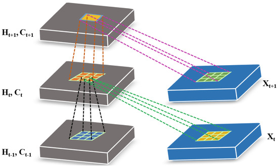
Figure 1.
The inner structure of ConvLSTM.
ConvLSTM includes three gates that complete data processing and transmission, making it more convenient to use spectral information of HSI. In contrast to CNN, which uses a sliding window to extract spatial information, the ConvLSTM implements the intra-layer data processing in addition to inter-layer processing. This is another significant difference from the CNN [53]. The unique design allows ConvLSTM to extract more powerful feature representations from sequential data.
3. Proposed Methodology
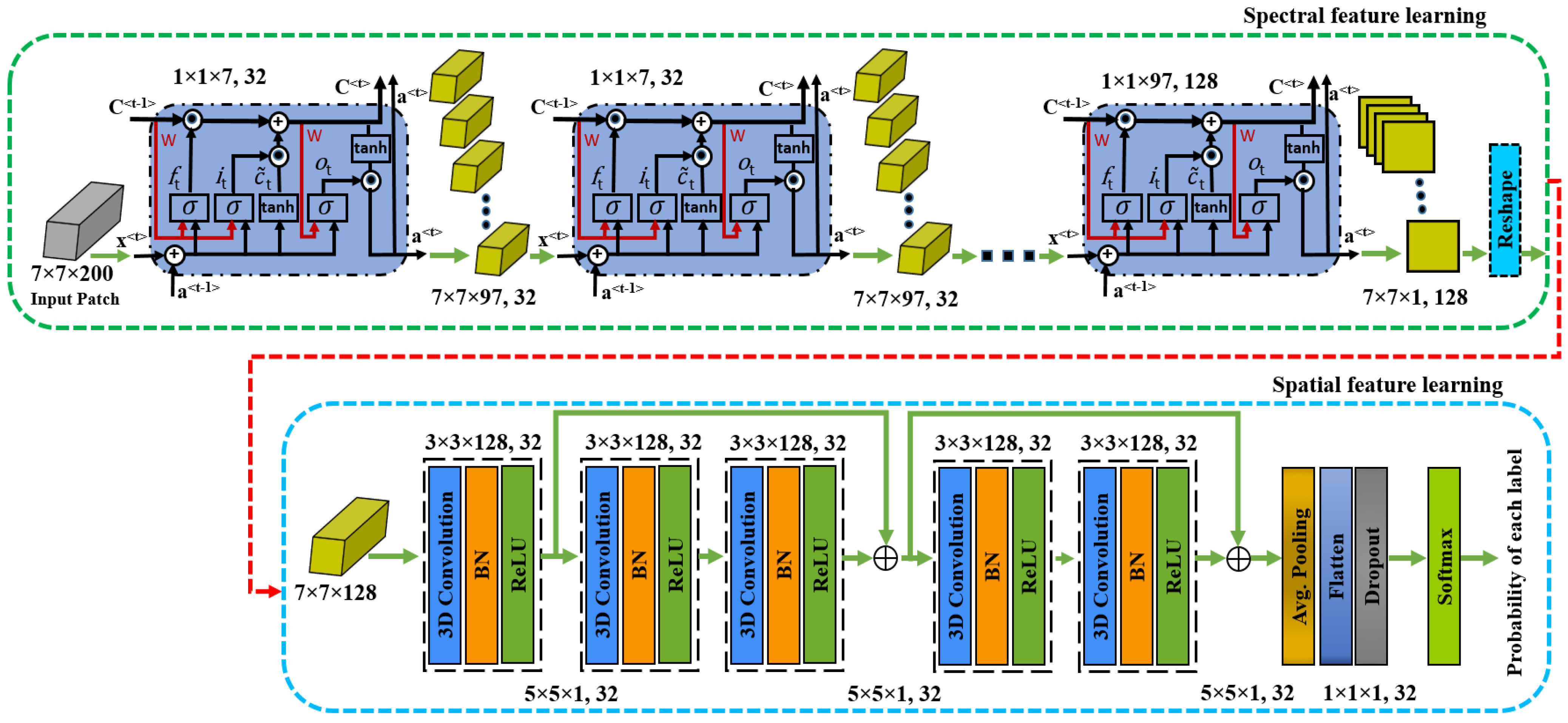
This section presents the proposed spectral–spatial 3D ConvLSTM-CNN based Residual Network (SSCRN) for HSI classification. The SSCRN takes into account both spectral and spatial domains and the universality of the HSIs. Precisely, the proposed architecture consists of two modules; i.e., 3D ConvLSTM and 3D CNN. The 3D ConvLSTM plays a role in learning robust spectral features, while 3D CNN aims to learn rich spatial features. The proposed architecture is shown in Figure 2 and explained in the subsequent sections.
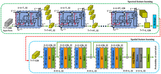
Figure 2.
The proposed spectral–spatial 3D ConvLSTM-CNN-based Residual Network (SSCRN). An HSI image is decomposed into a sequence of patches used as input to the ConvLSTM cell. The <t> represents the output/activation of the current cell/layer of the ConvLSTM, while <t−1> represents the output/activation of the previous layer.
3.1. 3D ConvLSTM Spectral Module
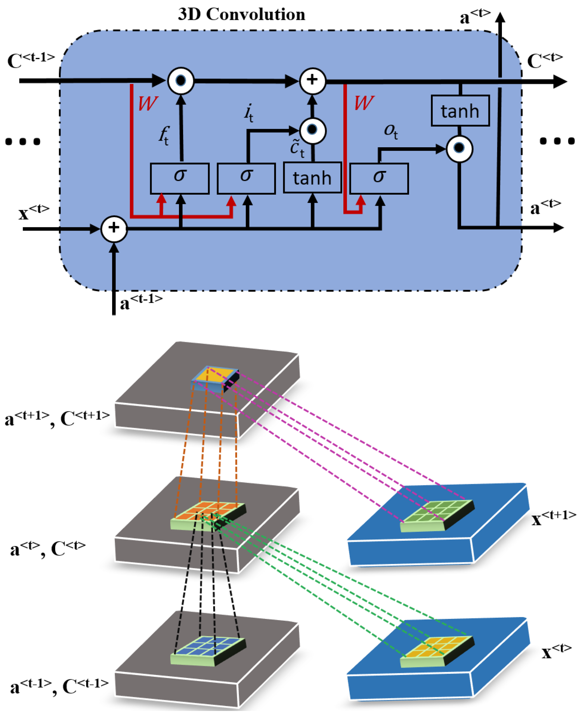
HSIs have many spectral bands, and some earlier methods [40] applied unsupervised principal component analysis (PCA) to acquire spectral features but could not obtain good results due to insufficient discriminative features [57]. On the other hand, 2D ConvLSTM can perform reasonably well for addressing the issue of long-term dependencies; however, it cannot handle 3D data cubes properly. Moreover, 2D models do not preserve the intrinsic structure of the 3D cubes when taking each band as an input for the corresponding memory cell [53]. This motivates us to employ 3D ConvLSTM for discriminative spectral feature extraction and preserve the intrinsic structure of the data. Generally, a 3D ConvLSTM is considered the extension of 2D ConvLSTM: it has three gates where 3D data is taken as input for each memory cell of the 3D ConvLSTM. Moreover, the convolutional kernel in 3D ConvLSTM is of shape , where and d are the kernel size and depth of the convolutional filter, respectively. The structure of the 3D ConvLSTM layer is shown in Figure 3. The equations of 3D ConvLSTM cell are written as
where , , , and are the input, forget, output gate, and memory cell, respectively. and are the input and output of the current memory cell, while and are the state and output of the previous memory cell. is a candidate for replacing the memory cell. “” and are activation functions, “*” is a convolution operator, and “∘” is a dot product, and , , , and are bias terms, as introduced in [51,58].
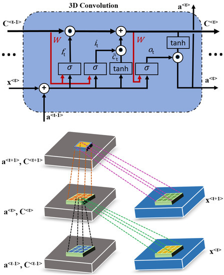
Figure 3.
The internal structure of 3D ConvLSTM.
More specifically, the input , the state and , the output and , and gate units , , and are 4D tensors with three spectral and two spatial dimensions, and the convolutional filters , , and are 3D tensors. “*” is a 3D convolution between 4D input or output and 3D convolution filters. ∈ is the input of the 3D ConvLSTM cell, which is the tth component in a sequence decomposed from the input of the 3D ConvLSTM according to the dimension , and ∈ , where , , , , , , and d are the dimension , width, height, number of the spectral band, kernel size and depth, respectively. Hence, the 3D convolution of and can be defined as *. The output can be defined as by at position in the input gate described as follows in Equation (5), and the value of is fixed as 1.
As represented above, the proposed spectral module can obtain the spectral features directly from HSI cubes. The unique structure of this module makes it an appropriate architecture for learning discriminative spectral features and preserving the intrinsic structure of data. This module is composed of four 3D ConvLSTM layers. In the first layer, a data patch of size is taken as an input. Then, 32 convolutional kernels of size with a stride of are convolved over the HSI patch to generate 32 feature columns with a size of as shown in Figure 2. Here, the convolution operation is performed only on the spectral channel, which also mitigates the redundant spectral information. The activation function for this layer is tanh, which is considered to be one of the most appropriate activations for LSTM layers with batch normalization. Next, the output of the first layer is passed to the second layer by applying the “same” padding to keep the input and output of the same size, while the rest of the settings are the same as the first layer. The output of the second layer is passed to the third layer, where the same settings are applied as layer 2. The last layer of the spectral module uses 128 convolution kernels of size in the Indian pines dataset, while for Salinas and the Pavia University, it becomes and , respectively. Finally, the output of the spectral module becomes the input for the spatial module for training the framework in an end-to-end fashion.
3.2. Deformable Process
The deformation process is required to convert the output of the spectral module into a 3D cube, making it suitable to be used as an input to the 3D CNN spatial module. In the spectral module discussed in Section 3.1, spectral feature maps are obtained with a size of . Then, these feature maps are reshaped into a cube to be used as an input to the spatial module, as depicted in Figure 4. The spatial module processes it further and learns the discriminative and robust spatial features for classification. This approach enables the effective combination of spectral and spatial information through an end-to-end framework, as shown in Figure 2.
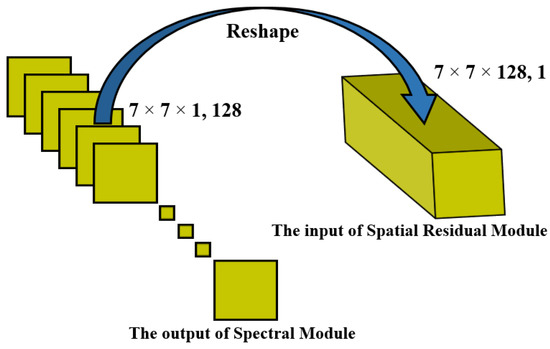
Figure 4.
Overview of deformable process.
3.3. Three-Dimensional CNN Spatial Residual Module
In this module, the 3D CNN layers are adopted as the basic building blocks of SSCRN, and batch normalization (BN) is applied after each layer. The BN makes the training process more efficient and smoother. A 3D CNN layer has input feature cubes of size with filters of size , and a stride of for the convolutional operation. Then, this layer generates an output of feature cubes of size , where the spatial width . The 3D CNN layer with BN can be represented as follows:
where is the lth input feature vector of ()th layer, is the normalization result of batch feature in the kth layer, and Std(.) and E(.) represent the standard deviation and expectation of the input feature vector, respectively. and denote the bias and weights of the ith filter in the (k + 1)th layer, represents the 3D convolution operator, and REL(.) is the activation function which transforms the negative numbers to zero.
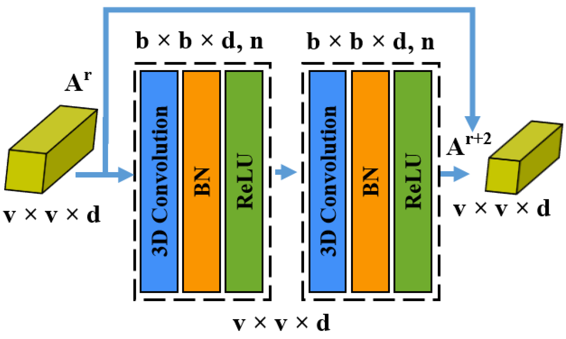
In the case of a large CNN, the accuracy begins to decrease after a few layers [39]. This issue may be addressed by creating residual blocks by introducing shortcut connections between layers [47]. In this direction, two residual blocks are meant to obtain spatial information, where each block is composed of two convolutional layers, as illustrated in Figure 5.
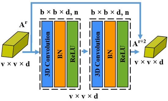
Figure 5.
The spatial residual block consists of two successive 3D CNN layers, and a skip connection to add input feature maps directly to the output feature maps .
There are five 3D convolutional layers, including an initial layer followed by two residual blocks; each layer is supported by batch normalization and the rectified linear unit (ReLU). This formulation allows gradients in higher layers to propagate back to lower layers to regularize and smooth the training process. The first convolutional layer receives an input from the spectral module discussed in Section 3.1, which has an input size of . Then, 32 kernels of size are applied. Here, q is the number of channels of this layer with a stride of , resulting in an output of feature maps. Then, two residual blocks, each with two convolutional layers, are used to learn spatial representations using 32 kernels of size at each layer. Here, the convolution operations are performed on spatial and spectral dimensions to carry on the complete information. After these residual blocks, an average pooling is applied to transform the obtained spectral–spatial feature volume to a feature vector. In addition to this, a dropout regularizer is also applied to address the overfitting problem. Subsequently, a fully connected (FC) layer receives input from the pooling layer and formulates a feature vector for classification. To validate the output produced by the model, a categorical cross-entropy loss is used, as shown in Equation (8). Finally, softmax layer activation is employed for the multi-class classification of different land cover categories.
where Y is the ground truth and is the corresponding predicted value by our proposed model.
4. Experimentations and Results Analysis
The proposed SSCRN is implemented in Keras and Tensorflow deep learning frameworks using the Python language. The results are generated on a Lenovo Legion Y7000 Intel Core i7-9750H gaming machine equipped with Nvidia GeForce RTX2060-6G and 32G memory. The proposed SSCRN model is evaluated using three evaluation metrics—i.e., overall accuracy , average accuracy , and kappa coefficient —while the higher values of , , and are considered better. Let V ∈ represent the error matrix classification results, where n indicates the number of land-cover categories and the value of V in position (i, j) represents the number of ith category samples classified to the jth category. The formulas for these metrics are shown in Equations (9)–(11).
where diag is a vector of diagonal values of V, is the sum of values, is the vector of the column-wise sum of all values, is the vector which shows the row-wise sum of all values, is the mean of all values, and shows the element-wise division.
4.1. Experimental Data Sets
The performance of SSCRN is evaluated on three well-known benchmark datasets: Indian Pines, Salinas, and Pavia University. The Indian Pines (IP) dataset was acquired by the Airborne Visible/Infrared Imaging Spectrometer (AVIRIS) sensor over diverse agricultural and forest areas. In this dataset, the spatial size of the scene is pixels, and the spatial resolution is 20 m per pixel (mpp). It contains 224 spectral bands across a wavelength ranging from 400 to 2500. In this experimentation, 200 bands are utilized after removing 24 noisy and zero-value bands. The land cover scene consists of 16 classes with 10,249 labeled pixels, where each class has different numbers of samples ranging from 20 to 2455. Each class’s samples are divided into training, validation, and test sets, as presented in Table 1.

Table 1.
Train, validation, and test split of IP dataset.
The Salinas (SA) is another important and well-known dataset used for hyperspectral image classification. An AVIRIS sensor was used to collect this dataset with 224 spectral bands over the Salinas Valley. Out of 224 spectral bands, 204 bands are utilized. This dataset has a spatial size of pixels with a spatial resolution of 3.7 mpp with 16 different land cover classes. The training, validation, and test split of samples is shown in Table 2.

Table 2.
Train, validation, and test split of SA dataset.
The Pavia University (PU) dataset was recorded by the reflective optics system imaging spectrometer (ROSIS) sensor over the University of Pavia. This dataset has 115 spectral bands; 103 bands are utilized after discarding noisy bands. The spatial size of this dataset is . There are nine classes with different numbers of samples, as listed in Table 3.

Table 3.
Train, validation and test split of PU dataset.
4.2. Experimental Settings
In the experimental setup, dataset division is considered an essential factor for the system’s performance. For this purpose, a train/validation/test split strategy is selected to evaluate the proposed model. In the case of SA and PU datasets, 5%, 5%, and 90% split ratios are used for training, validation, and test, respectively, while for the IP dataset, the ratio was 10%:10%:80%. Further, the detailed information is given in Table 1, Table 2 and Table 3. Another important factor is the proper selection and tuning of hyperparameters of the model. Although all parameters are not equally important, appropriate values of parameters always lead to a balanced model. The important hyperparameters used in the proposed model are batch size, learning rate, regularizers, optimizers, and number of epochs. There are two well-known strategies for tuning parameters: grid search and random search. A random search is more suitable for deep learning models due to its capability to explore greater numbers of relevant parameter values. Therefore, a random search strategy has been adopted to find appropriate values for the hyperparameters used in the model. The appropriate value for the batch size is 32 for IP and 64 for SA and PU datasets.
In this way, among different optimizers, Adam [59] was selected for optimizing the model based on the tuning process. During optimization, the learning rate is considered one of the most important hyperparameters; its appropriate value plays an important role in the model’s convergence. Consequently, optimal learning rates for IP, SA, and PU datasets are 0.0003, 0.0001, and 0.0001, respectively. Moreover, batch normalization and dropout are used during the training process to avoid overfitting. The proposed model was also assessed with and without regularization methods. The results confirm that regularizing methods help to achieve better performance, as shown in Table 4. The network and parameter settings for the proposed SSCRN framework are summarized in Table 5. Moreover, the detailed comparison for hyperparameters of the proposed method against state-of-the-art techniques is presented in Table 6.

Table 4.
OA accuracy of SSCRN with different regularizers.

Table 5.
Network topology of the proposed SSCRN model.

Table 6.
Comparison of hyperparameters with state-of-the-art methods.
4.3. Classification Results
The proposed model is compared with several state-of-the-art models to prove its efficacy, including SVM [60,61], 3D-CNN [31], BASSNet [62], 2D–3D CNN [63], SS3FCN [10], ADR-3D-CNN [64], FCLFN [65], FFDN-SY [66], and TAP-Net [67]. It is worth noting that the proposed model achieved superior performance with a smaller or equivalent amount of training data compared to other state-of-the-art techniques except [65], as presented in Table 7, Table 8 and Table 9.

Table 7.
Classification results (%) of different methods on the IP dataset. Bold indicates the best accuracy.

Table 8.
Classification results (%) of different methods on the SA dataset. Bold indicates the best accuracy.

Table 9.
Classification results (%) of different methods on the PU dataset. Bold indicates the best accuracy.
The first experiment was performed on the IP dataset. Some classes have few samples in this dataset, making it challenging for classification due to the imbalanced class problem. Therefore, existing methods have either excluded these classes from their experiments or have shown poor performance, as evident from Table 7. Despite the fact, SSCRN demonstrated 100% accurate results for these classes, which are “Oats”, “Grass-p-m”, and “Alfafa”. Moreover, across all evaluation measures—i.e., OA, AA, and kappa coefficient—the SSCRN performed better than the compared methods with an OA of 99.17%, as presented in Table 7.
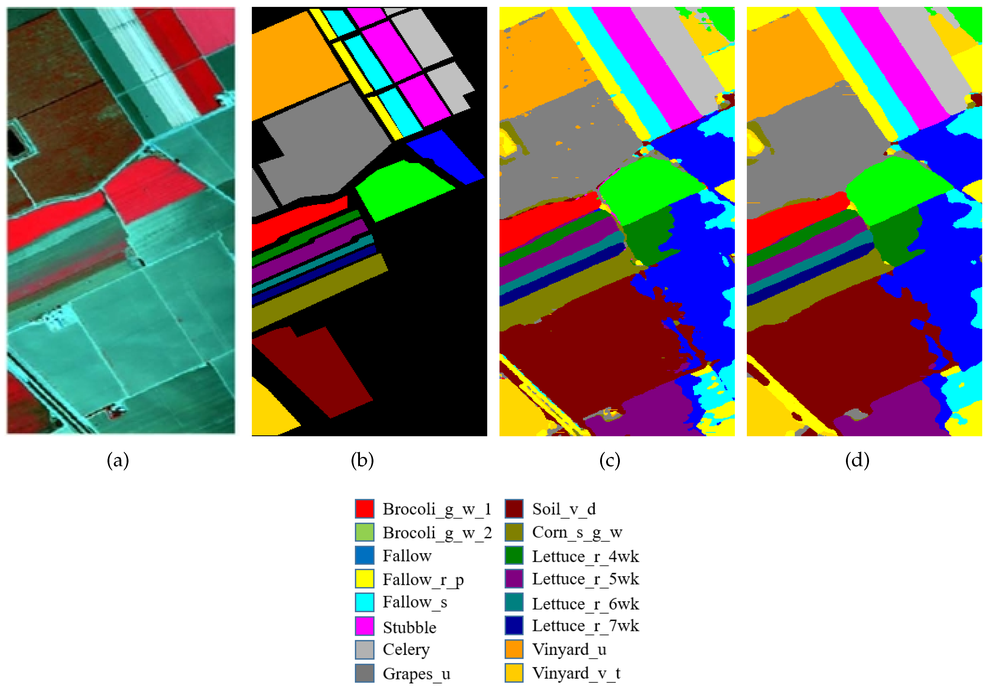
The second experiment was performed on the SA dataset. The SSCRN achieved an accuracy of 100% in the “Brocoli_g_w_2”, “Fallow”, “Fallow_s”, “Stubble”, “Celery”, “Lettuce_r_6wk”, and “Vinyard_v_t” categories. Moreover, across all evaluation measures—i.e., OA, AA, and kappa coefficient—the SSCRN performed better than state-of-the-art methods with an overall accuracy of 99.67%, as shown in Table 8.
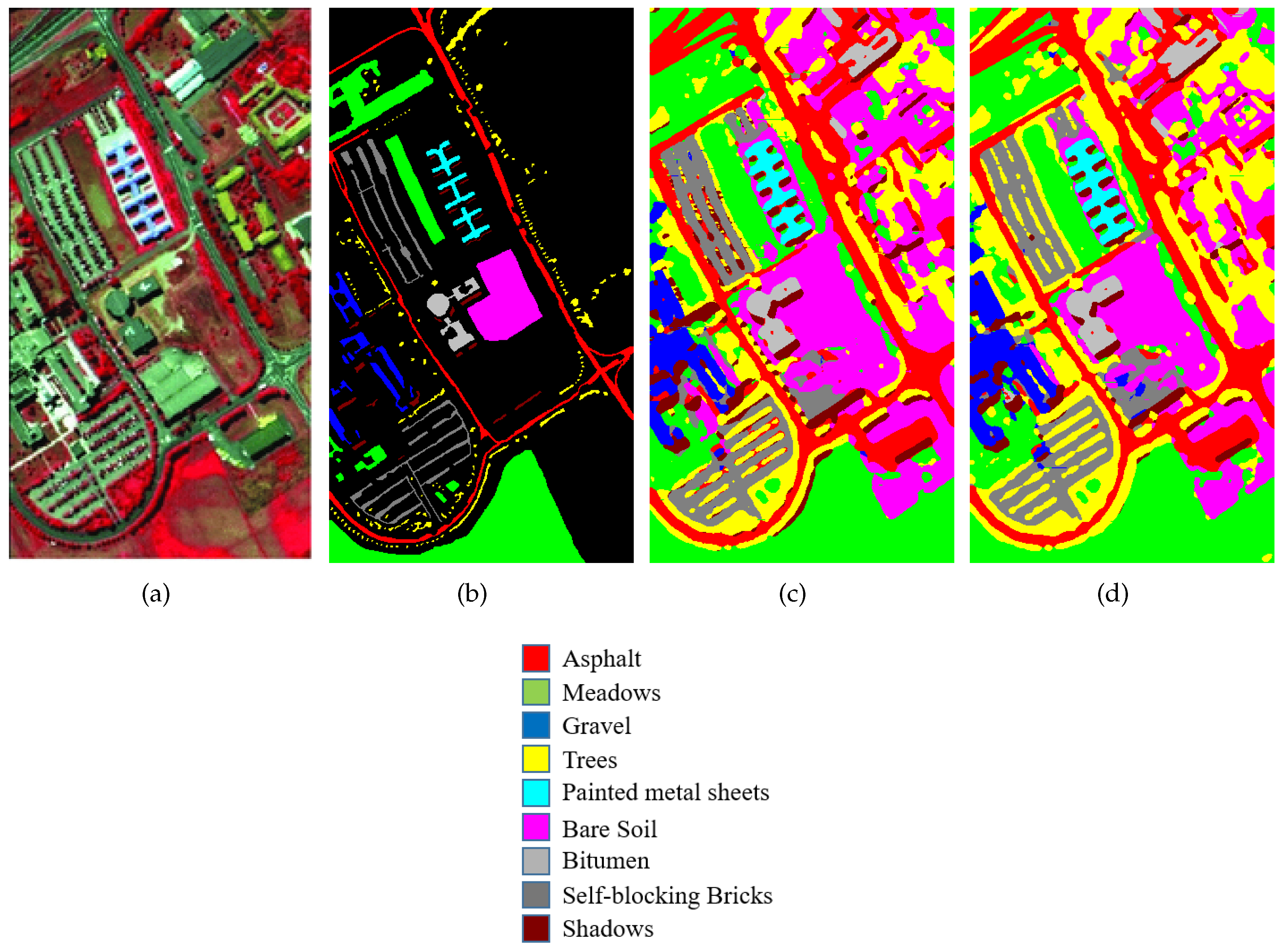
The third experiment was conducted on the PU dataset. Compared with the IP dataset, this dataset has a relatively large number of training samples for each category with nine classes, while the IP has 16 classes. Due to sufficient training samples, many deep learning models have achieved better performance on this dataset. However, due to interfering pixels, extracting discriminative features is still a challenging task for this dataset. The SSCRN produced excellent results on this dataset, as shown in Table 9.
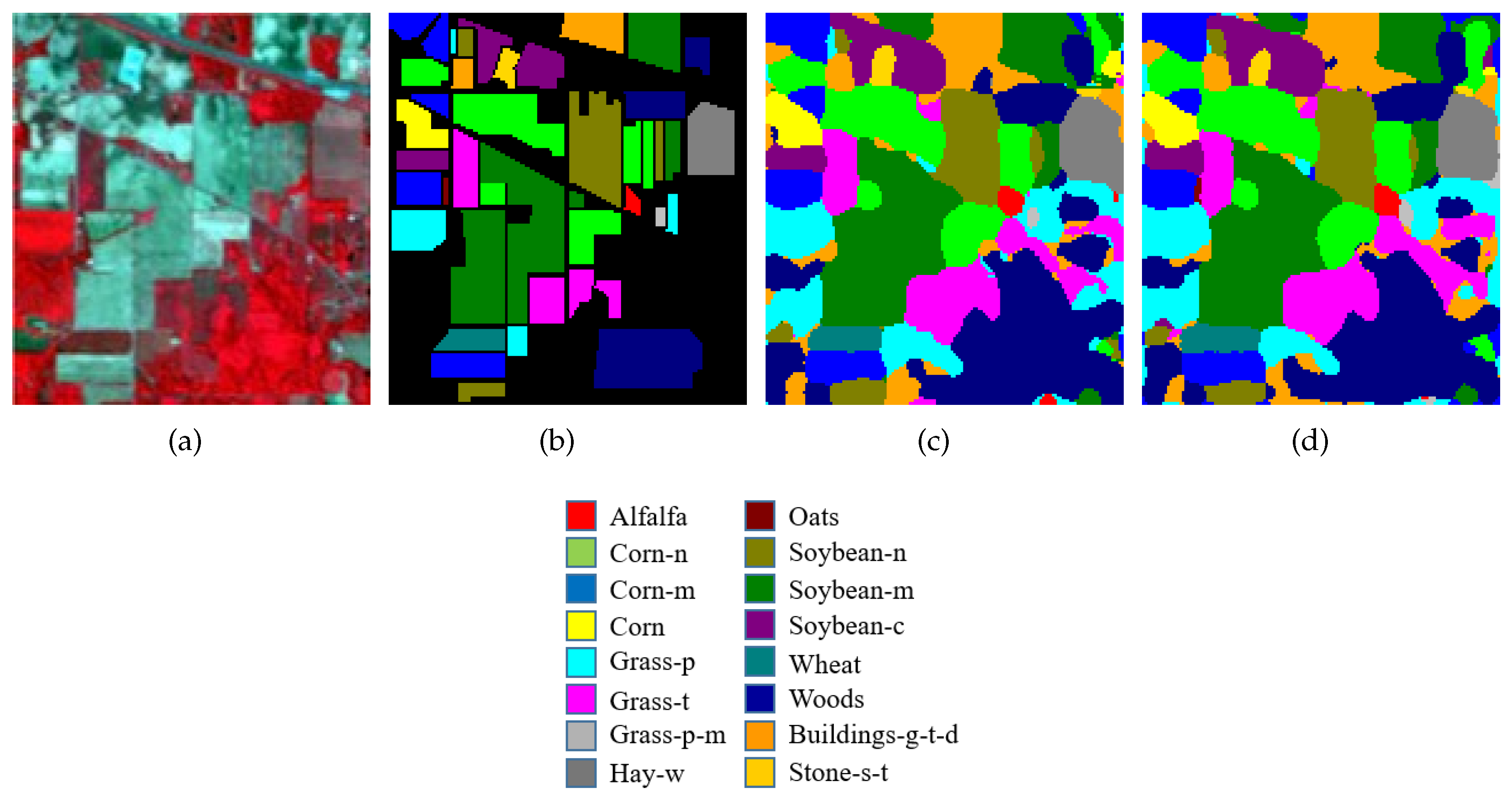
For better understanding, the visual classification results for each dataset are presented in Figure 6, Figure 7 and Figure 8 with false color images and their corresponding ground-truth maps. These maps also confirm the outstanding performance of SSCRN on the three HSI datasets discussed above. In particular, the SSCRN performed exceptionally well at the edges of land-cover areas and alleviated the effect of interfering pixels. In addition to this, it also suppressed spectral variability and produced smooth visual maps.
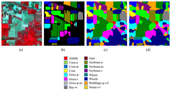
Figure 6.
Visual classification results on the IP dataset. (a) A three-band color composite image, (b) the ground-truth image. Classification results of input image patch size (c) , (d) .

Figure 7.
Visual classification results on the SA. (a) A three-band color composite image, (b) the ground-truth image. Classification results of input image patch size (c) , (d) .
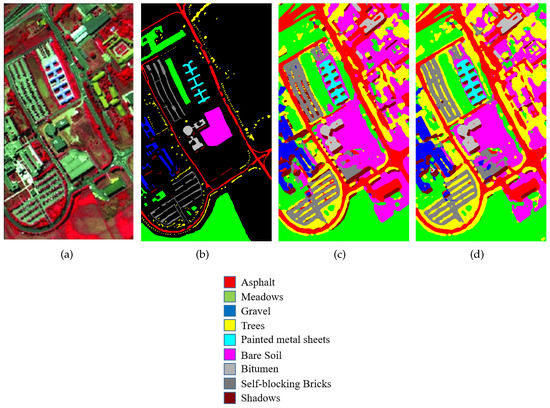
Figure 8.
Visual classification results on the PU dataset. (a) A three-band color composite image, (b) the ground-truth image. Classification results of input image patch size (c) , (d) .
4.4. Impact of Training Ratio
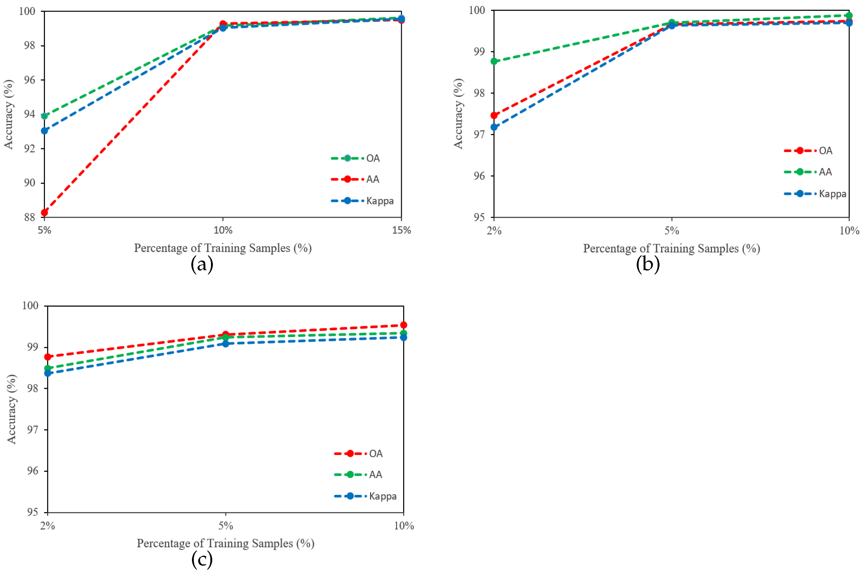
The robustness and generalizability of the SSCRN were evaluated with a varying number of training samples from each dataset. In this regard, 5%, 10%, and 15% of the total samples were used from the IP dataset, and 2%, 5%, and 10% for the SA and PU datasets. The OA of SSCRN using different numbers of training samples is reported in Figure 9, which shows that a larger number of samples leads to higher accuracy.
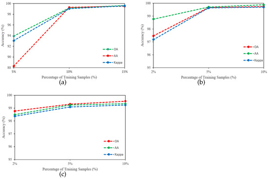
Figure 9.
Accuracy (%) of SSCRN with different training percentages on three datasets: (a) IP, (b) SA, (c) PU.
4.5. Impact of Spatial Size of the Input Image Patches
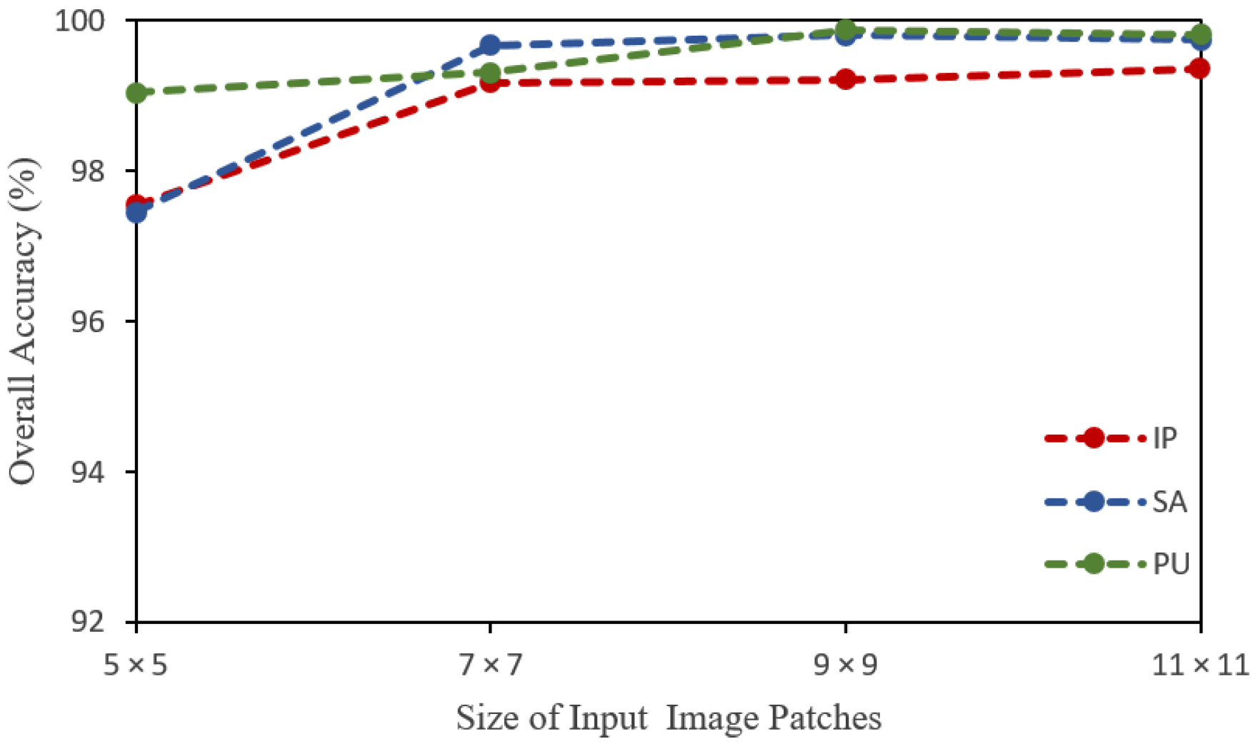
The proposed model was also evaluated with different input patch sizes to assess the impact of input patches and find their optimal size. In this regard, the patch sizes of , , , and were employed. It has been learned that a larger input patch size results in higher classification accuracy, which is quite reasonable because a larger spatial size contains more information. The larger patch size provides higher accuracy but at the cost of computational complexity. In this regard, we selected a spatial size of , which provides a good balance between high performance and computational complexity. The results with different patch sizes are presented in Figure 10 and Table 10.
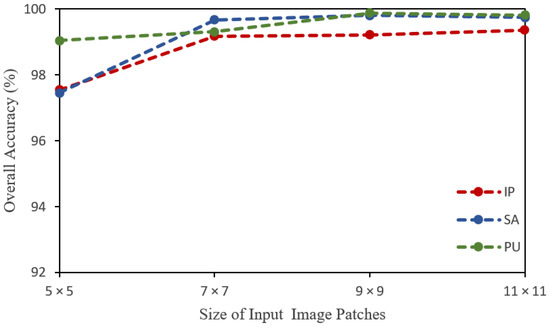
Figure 10.
Overall accuracy (%) along with varying sizes of input image patches on IP, SA, and PU datasets.

Table 10.
Accuracy (%) of SSCRN under different spatial sizes of the input image patches on different datasets. Bold indicates the best accuracy.
4.6. Impact of the Number of Convolution Kernels
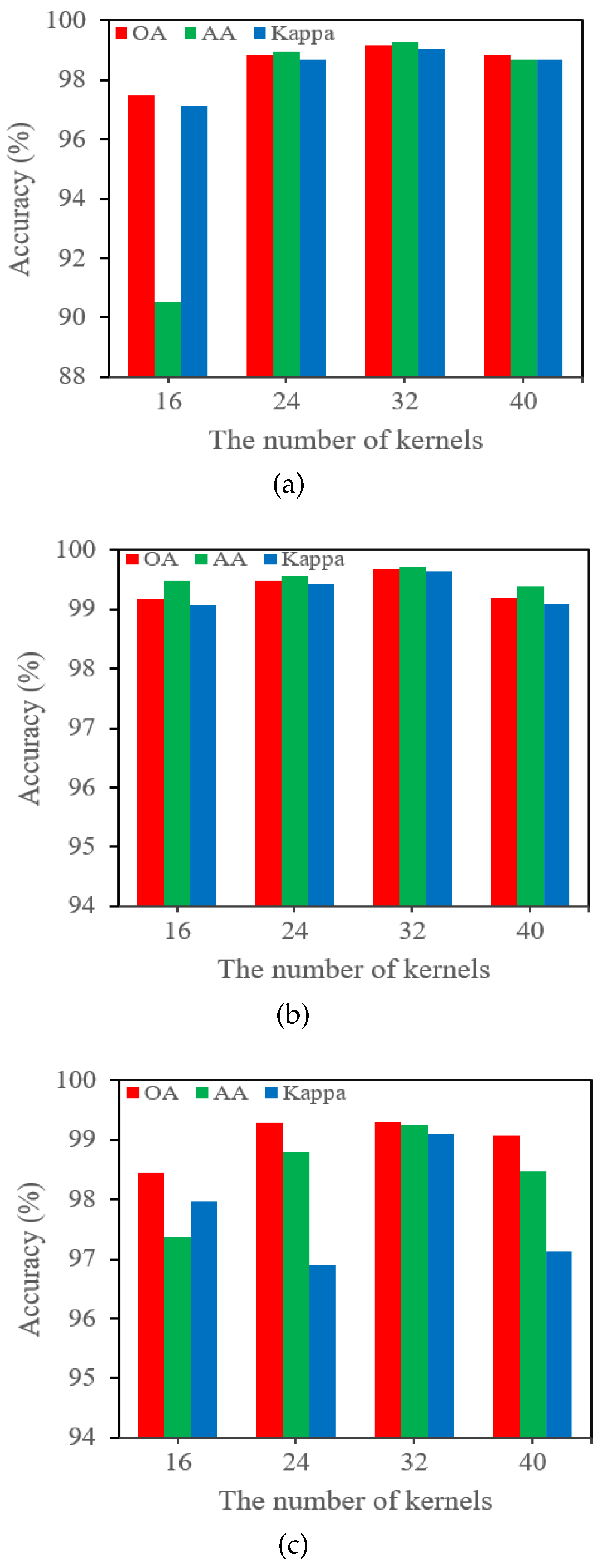
The number of convolution kernels in a network determines its computational complexity and representation capacity. As illustrated in Figure 2, the SSCRN employs the same number of kernels in both the spectral and spatial modules. In order to evaluate the effect of varying numbers of kernels on the accuracy, different numbers of kernels such as 16, 24, 32, and 40 are applied in each layer, as shown in Figure 11. The highest accuracy is achieved using 32 kernels in each layer in the case of all three datasets. Figure 11a represents the detailed classification results on the IP dataset in terms of OA, AA, and kappa. Likewise, Figure 11b shows the detailed classification results of the SA dataset, and Figure 11c illustrates the classification results on the PU dataset.
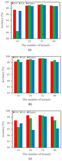
Figure 11.
Accuracy (%) of SSCRN with different numbers of kernels on three datasets: (a) IP, (b) SA, (c) PU.
4.7. Ablation Study
Although the SSCRN in its current form has proved to be effective for discriminative feature learning and HSI classification, an ablation study was performed to confirm the proposed model’s robustness and generalization ability with different variations. For this purpose, the order of spectral and spatial modules was swapped. As a result of this change, the model first learned the spatial features using 3D CNN with residual blocks and then spectral features by employing the 3D ConvLSTM. The results confirm that the model also performed well with this arrangement of modules, but the accuracy was slightly decreased compared to its original version, as shown in Table 11. Moreover, it can also be concluded that arranging modules in a spectral–spatial fashion is superior to its spatial–spectral counterpart.

Table 11.
Ablation study of swapping the sequence of spectral and spatial modules of SSCRN.
5. Discussion
Compared to traditional state-of-the-art approaches, deep learning-based techniques offer several benefits: automatic feature extraction from HSI data, hierarchical nonlinear transformation, objective functions that focus exclusively on classification rather than two independent steps, and the efficient use of computational resources such as GPU [39]. The proposed SSCRN harnesses the potential of 3D ConvLSTM and 3D CNN, which are considered excellent frameworks for different computer vision tasks, including HSI classification. However, the proposed SSCRN is significantly different from the existing techniques. There are four significant differences between SSCRN and other deep learning models. First, the SSCRN separates spectral and spatial features into two consecutive modules: 3D ConvLSTM and 3D CNN. The 3D ConvLSTM module aims to learn the robust spectral feature representations, and the 3D CNN learns spatial features. This allows for better discriminative features to be retrieved consecutively and reduces the chance of information loss. Second, the SSCRN employs residual connections to ensure that the network can work more deeply to enhance classification accuracy and avoid overfitting. Third, utilizing a BN operation at each layer, the model’s fast learning capability can be ensured, and the model converges in fewer epochs. Fourth, the proposed SSCRN model achieved high classification accuracy, especially for the classes with few training samples. It is worth noting that, in this study, data augmentation [37] was not employed to increase the number of training samples; still, the model achieved excellent performance, which confirms the robustness of the SSCRN.
It has been learned that three key factors influence the performance of supervised deep learning models in terms of HSI classifications: (1) the spatial size of the input image patch, (2) the number of training samples, and (3) the representation ability of the proposed model. A greater number of training samples and a larger patch size lead to higher classification accuracy. Hence, the same number of training samples must be used for a fair comparison. For further clarification, the performance of SSCRN with different numbers of training samples and patch sizes were reported for three datasets, as shown in Figure 9 and Figure 10. It has been observed that the performance in terms of OA declines with a reduction in the number of training samples and the patch size.
6. Conclusions
This paper presented a novel supervised deep learning framework consisting of two modules—i.e., a 3D ConvLSTM followed by a 3D CNN with residual blocks—to learn discriminative spectral–spatial representations for HSI classification. The input of the 3D ConvLSTM module was a sequence of local data patches fed into each memory cell to learn effective features and model long-term dependencies in the spectral domain. The output of the spectral module was converted into a 3D cube by applying a special transformation process, making it suitable for the 3D CNN spatial module. The 3D CNN spatial module was designed to extract robust features in the spatial context. This module employed the concept of skip connections similar to residual blocks to accelrate the training process and avoid overfitting. Then, fused spectral and spatial information was used for final classification. The proposed method achieved excellent results on three benchmark datasets, with an overall accuracy of 99.17%, 99.67%, 99.31% and the average accuracy of 99.29%, 99.71%, and 99.24% over Indian Pines, Salinas, and Pavia University datasets, respectively. The major advantage of the SSCRN is that it can be generalized to other remote sensing problems due to its robust design and in-depth feature learning capacity. However, it has been observed that the performance in terms of OA declines with a reduction in the number of training samples and the input image patch size. One of the possible extension of this work could be to make it computationally lean and achieve better accuracy with a reduced number of training samples and smaller patch size.
Author Contributions
G.F. and A.B.S. conceived and designed the experiments; G.F. performed the experiments. A.B.S. and G.F. analyzed the results; G.F. wrote the paper; A.B.S. improved the manuscript grammatically; J.Y. revised the manuscript; L.X. supervised and provided insightful advice to this study and revised the manuscript. All authors have read and agreed to the published version of the manuscript.
Funding
This work was supported in part by the National Natural Science Foundation of China (Grants No. 61871226, 61571230), the Jiangsu Provincial Social Developing Project (Grant No. BE2018727).
Data Availability Statement
The HSI datasets used in this study are freely available at http://www.ehu.eus/ccwintco/index.php/Hyperspectral_Remote_Sensing_Scenes (accessed on 30 August 2021).
Conflicts of Interest
The authors declare no conflict of interest.
References
- Khan, M.J.; Khan, H.S.; Yousaf, A.; Khurshid, K.; Abbas, A. Modern trends in hyperspectral image analysis: A review. IEEE Access 2018, 6, 14118–14129. [Google Scholar] [CrossRef]
- Wang, Q.; Yuan, Z.; Du, Q.; Li, X. GETNET: A general end-to-end 2-D CNN framework for hyperspectral image change detection. IEEE Trans. Geosci. Remote Sens. 2018, 57, 3–13. [Google Scholar] [CrossRef] [Green Version]
- Sun, H.; Zheng, X.; Lu, X.; Wu, S. Spectral-Spatial Attention Network for Hyperspectral Image Classification. IEEE Trans. Geosci. Remote Sens. 2019, 58, 3232–3245. [Google Scholar] [CrossRef]
- Maes, W.H.; Steppe, K. Perspectives for remote sensing with unmanned aerial vehicles in precision agriculture. Trends Plant Sci. 2019, 24, 152–164. [Google Scholar] [CrossRef] [PubMed]
- Tan, Y.; Lu, L.; Bruzzone, L.; Guan, R.; Chang, Z.; Yang, C. Hyperspectral Band Selection for Lithologic Discrimination and Geological Mapping. IEEE J. Sel. Top. Appl. Earth Obs. Remote Sens. 2020, 13, 471–486. [Google Scholar] [CrossRef]
- Yousefi, B.; Castanedo, C.I.; Bédard, É.; Beaudoin, G.; Maldague, X.P. Mineral identification in LWIR hyperspectral imagery applying sparse-based clustering. Quant. Infrared Thermogr. J. 2019, 16, 147–162. [Google Scholar] [CrossRef]
- Shimoni, M.; Haelterman, R.; Perneel, C. Hypersectral Imaging for Military and Security Applications: Combining Myriad Processing and Sensing Techniques. IEEE Geosci. Remote Sens. Mag. 2019, 7, 101–117. [Google Scholar] [CrossRef]
- Stuart, M.B.; McGonigle, A.J.; Willmott, J.R. Hyperspectral Imaging in Environmental Monitoring: A Review of Recent Developments and Technological Advances in Compact Field Deployable Systems. Sensors 2019, 19, 3071. [Google Scholar] [CrossRef] [PubMed] [Green Version]
- Wu, P.; Cui, Z.; Gan, Z.; Liu, F. Three-Dimensional ResNeXt Network Using Feature Fusion and Label Smoothing for Hyperspectral Image Classification. Sensors 2020, 20, 1652. [Google Scholar] [CrossRef] [PubMed] [Green Version]
- Zou, L.; Zhu, X.; Wu, C.; Liu, Y.; Qu, L. Spectral–Spatial Exploration for Hyperspectral Image Classification via the Fusion of Fully Convolutional Networks. IEEE J. Sel. Top. Appl. Earth Obs. Remote Sens. 2020, 13, 659–674. [Google Scholar] [CrossRef]
- Gan, Y.; Luo, F.; Liu, J.; Lei, B.; Zhang, T.; Liu, K. Feature extraction based multi-structure manifold embedding for hyperspectral remote sensing image classification. IEEE Access 2017, 5, 25069–25080. [Google Scholar] [CrossRef]
- Fauvel, M.; Tarabalka, Y.; Benediktsson, J.A.; Chanussot, J.; Tilton, J.C. Advances in spectral-spatial classification of hyperspectral images. Proc. IEEE 2012, 101, 652–675. [Google Scholar] [CrossRef] [Green Version]
- Belgiu, M.; Drăguţ, L. Random forest in remote sensing: A review of applications and future directions. ISPRS J. Photogramm. Remote Sens. 2016, 114, 24–31. [Google Scholar] [CrossRef]
- Jia, S.; Hu, J.; Zhu, J.; Jia, X.; Li, Q. Three-dimensional local binary patterns for hyperspectral imagery classification. IEEE Trans. Geosci. Remote Sens. 2017, 55, 2399–2413. [Google Scholar] [CrossRef]
- Xu, Y.; Wu, Z.; Wei, Z. Markov random field with homogeneous areas priors for hyperspectral image classification. In Proceedings of the 2014 IEEE Geoscience and Remote Sensing Symposium, Quebec City, QC, Canada, 13–18 July 2014; pp. 3426–3429. [Google Scholar]
- Quesada-Barriuso, P.; Argüello, F.; Heras, D.B. Spectral–Spatial classification of hyperspectral images using wavelets and extended morphological profiles. IEEE J. Sel. Top. Appl. Earth Obs. Remote Sens. 2014, 7, 1177–1185. [Google Scholar] [CrossRef]
- He, L.; Chen, X. A three-dimensional filtering method for spectral-spatial hyperspectral image classification. In Proceedings of the 2016 IEEE International Geoscience and Remote Sensing Symposium (IGARSS), Beijing, China, 10–15 July 2016; pp. 2746–2748. [Google Scholar]
- Bau, T.C.; Sarkar, S.; Healey, G. Hyperspectral region classification using a three-dimensional Gabor filterbank. IEEE Trans. Geosci. Remote Sens. 2010, 48, 3457–3464. [Google Scholar] [CrossRef]
- Yin, J.; Li, S.; Zhu, H.; Luo, X. Hyperspectral image classification using CapsNet with well-initialized shallow layers. IEEE Geosci. Remote Sens. Lett. 2019, 16, 1095–1099. [Google Scholar] [CrossRef]
- Zhang, L.; Zhang, L.; Du, B. Deep learning for remote sensing data: A technical tutorial on the state of the art. IEEE Geosci. Remote Sens. Mag. 2016, 4, 22–40. [Google Scholar] [CrossRef]
- Ma, A.; Filippi, A.M.; Wang, Z.; Yin, Z. Hyperspectral image classification using similarity measurements-based deep recurrent neural networks. Remote Sens. 2019, 11, 194. [Google Scholar] [CrossRef] [Green Version]
- Zhang, M.; Li, W.; Du, Q.; Gao, L.; Zhang, B. Feature extraction for classification of hyperspectral and LiDAR data using patch-to-patch CNN. IEEE Trans. Cybern. 2018, 50, 100–111. [Google Scholar] [CrossRef] [PubMed]
- Mustaqeem; Kwon, S. 1D-CNN: Speech Emotion Recognition System Using a Stacked Network with Dilated CNN Features. CMC-Comput. Mater. Contin. 2021, 67, 4039–4059. [Google Scholar] [CrossRef]
- Sargano, A.B.; Wang, X.; Angelov, P.; Habib, Z. Human action recognition using transfer learning with deep representations. In Proceedings of the 2017 International joint conference on neural networks (IJCNN), Anchorage, AK, USA, 14–19 May 2017; pp. 463–469. [Google Scholar]
- Farooque, G.; Sargano, A.B.; Shafi, I.; Ali, W. Coin recognition with reduced feature set sift algorithm using neural network. In Proceedings of the 2016 International Conference on Frontiers of Information Technology (FIT), Islamabad, Pakistan, 19–21 December 2016; pp. 93–98. [Google Scholar]
- Ashraf, M.; Geng, G.; Wang, X.; Ahmad, F.; Abid, F. A Globally Regularized Joint Neural Architecture for Music Classification. IEEE Access 2020, 8, 220980–220989. [Google Scholar] [CrossRef]
- Chen, Y.; Lin, Z.; Zhao, X.; Wang, G.; Gu, Y. Deep learning-based classification of hyperspectral data. IEEE J. Sel. Top. Appl. Earth Obs. Remote Sens. 2014, 7, 2094–2107. [Google Scholar] [CrossRef]
- Chen, Y.; Zhao, X.; Jia, X. Spectral–spatial classification of hyperspectral data based on deep belief network. IEEE J. Sel. Top. Appl. Earth Obs. Remote Sens. 2015, 8, 2381–2392. [Google Scholar] [CrossRef]
- Mou, L.; Ghamisi, P.; Zhu, X.X. Deep recurrent neural networks for hyperspectral image classification. IEEE Trans. Geosci. Remote Sens. 2017, 55, 3639–3655. [Google Scholar] [CrossRef] [Green Version]
- Yang, J.; Zhao, Y.Q.; Chan, J.C.W. Learning and transferring deep joint spectral–spatial features for hyperspectral classification. IEEE Trans. Geosci. Remote Sens. 2017, 55, 4729–4742. [Google Scholar] [CrossRef]
- Lee, H.; Kwon, H. Going deeper with contextual CNN for hyperspectral image classification. IEEE Trans. Image Process. 2017, 26, 4843–4855. [Google Scholar] [CrossRef] [PubMed] [Green Version]
- Zhao, W.; Du, S. Spectral–spatial feature extraction for hyperspectral image classification: A dimension reduction and deep learning approach. IEEE Trans. Geosci. Remote Sens. 2016, 54, 4544–4554. [Google Scholar] [CrossRef]
- Liu, B.; Yu, X.; Zhang, P.; Yu, A.; Fu, Q.; Wei, X. Supervised deep feature extraction for hyperspectral image classification. IEEE Trans. Geosci. Remote Sens. 2017, 56, 1909–1921. [Google Scholar] [CrossRef]
- Feng, F.; Wang, S.; Wang, C.; Zhang, J. Learning Deep Hierarchical Spatial–Spectral Features for Hyperspectral Image Classification Based on Residual 3D-2D CNN. Sensors 2019, 19, 5276. [Google Scholar] [CrossRef] [PubMed] [Green Version]
- Jia, S.; Zhao, B.; Tang, L.; Feng, F.; Wang, W. Spectral–spatial classification of hyperspectral remote sensing image based on capsule network. J. Eng. 2019, 2019, 7352–7355. [Google Scholar] [CrossRef]
- Li, X.; Ding, M.; Pižurica, A. Deep Feature Fusion via Two-Stream Convolutional Neural Network for Hyperspectral Image Classification. IEEE Trans. Geosci. Remote Sens. 2019, 58, 2615–2629. [Google Scholar] [CrossRef] [Green Version]
- Chen, Y.; Jiang, H.; Li, C.; Jia, X.; Ghamisi, P. Deep feature extraction and classification of hyperspectral images based on convolutional neural networks. IEEE Trans. Geosci. Remote Sens. 2016, 54, 6232–6251. [Google Scholar] [CrossRef] [Green Version]
- Li, Y.; Zhang, H.; Shen, Q. Spectral–spatial classification of hyperspectral imagery with 3D convolutional neural network. Remote Sens. 2017, 9, 67. [Google Scholar] [CrossRef] [Green Version]
- Zhong, Z.; Li, J.; Luo, Z.; Chapman, M. Spectral–spatial residual network for hyperspectral image classification: A 3-D deep learning framework. IEEE Trans. Geosci. Remote Sens. 2017, 56, 847–858. [Google Scholar] [CrossRef]
- Song, W.; Li, S.; Fang, L.; Lu, T. Hyperspectral image classification with deep feature fusion network. IEEE Trans. Geosci. Remote Sens. 2018, 56, 3173–3184. [Google Scholar] [CrossRef]
- Zhang, C.; Li, G.; Du, S.; Tan, W.; Gao, F. Three-dimensional densely connected convolutional network for hyperspectral remote sensing image classification. J. Appl. Remote Sens. 2019, 13, 016519. [Google Scholar] [CrossRef]
- Liu, Q.; Xiao, L.; Yang, J.; Chan, J.C.W. Content-guided convolutional neural network for hyperspectral image classification. IEEE Trans. Geosci. Remote Sens. 2020, 58, 6124–6137. [Google Scholar] [CrossRef]
- Liu, Q.; Xiao, L.; Yang, J.; Wei, Z. CNN-enhanced graph convolutional network with pixel-and superpixel-level feature fusion for hyperspectral image classification. IEEE Trans. Geosci. Remote Sens. 2020, 59, 8657–8671. [Google Scholar] [CrossRef]
- Fang, B.; Li, Y.; Zhang, H.; Chan, J.C.W. Hyperspectral images classification based on dense convolutional networks with spectral-wise attention mechanism. Remote Sens. 2019, 11, 159. [Google Scholar] [CrossRef] [Green Version]
- Xu, Q.; Xiao, Y.; Wang, D.; Luo, B. CSA-MSO3DCNN: Multiscale Octave 3D CNN with Channel and Spatial Attention for Hyperspectral Image Classification. Remote Sens. 2020, 12, 188. [Google Scholar] [CrossRef] [Green Version]
- Jamshidpour, N.; Aria, E.H.; Safari, A.; Homayouni, S. Adaptive Self-Learned Active Learning Framework for Hyperspectral Classification. In Proceedings of the 10th Workshop on Hyperspectral Imaging and Signal Processing: Evolution in Remote Sensing (WHISPERS), Amsterdam, The Netherlands, 24–26 September 2019; pp. 1–5. [Google Scholar]
- He, K.; Zhang, X.; Ren, S.; Sun, J. Deep residual learning for image recognition. In Proceedings of the IEEE Conference on Computer Vision and Pattern Recognition, Las Vegas, NV, USA, 27–30 June 2016; pp. 770–778. [Google Scholar]
- Ienco, D.; Gaetano, R.; Dupaquier, C.; Maurel, P. Land cover classification via multitemporal spatial data by deep recurrent neural networks. IEEE Geosci. Remote Sens. Lett. 2017, 14, 1685–1689. [Google Scholar] [CrossRef] [Green Version]
- Zhou, F.; Hang, R.; Liu, Q.; Yuan, X. Hyperspectral image classification using spectral-spatial LSTMs. Neurocomputing 2019, 328, 39–47. [Google Scholar] [CrossRef]
- Kwon, S. CLSTM: Deep feature-based speech emotion recognition using the hierarchical ConvLSTM network. Mathematics 2020, 8, 2133. [Google Scholar]
- Xingjian, S.; Chen, Z.; Wang, H.; Yeung, D.Y.; Wong, W.K.; Woo, W.C. Convolutional LSTM network: A machine learning approach for precipitation nowcasting. In Proceedings of the Advances in Neural Information Processing Systems, Montreal, QC, Canada, 7–12 December 2015; pp. 802–810. [Google Scholar]
- Liu, Q.; Zhou, F.; Hang, R.; Yuan, X. Bidirectional-convolutional LSTM based spectral-spatial feature learning for hyperspectral image classification. Remote Sens. 2017, 9, 1330. [Google Scholar] [CrossRef] [Green Version]
- Hu, W.S.; Li, H.C.; Pan, L.; Li, W.; Tao, R.; Du, Q. Feature extraction and classification based on spatial-spectral convlstm neural network for hyperspectral images. arXiv 2019, arXiv:1905.03577. [Google Scholar]
- Bioucas-Dias, J.M.; Plaza, A.; Camps-Valls, G.; Scheunders, P.; Nasrabadi, N.; Chanussot, J. Hyperspectral remote sensing data analysis and future challenges. IEEE Geosci. Remote Sens. Mag. 2013, 1, 6–36. [Google Scholar] [CrossRef] [Green Version]
- Liu, S.; Marinelli, D.; Bruzzone, L.; Bovolo, F. A review of change detection in multitemporal hyperspectral images: Current techniques, applications, and challenges. IEEE Geosci. Remote Sens. Mag. 2019, 7, 140–158. [Google Scholar] [CrossRef]
- Hochreiter, S.; Schmidhuber, J. Long short-term memory. Neural Comput. 1997, 9, 1735–1780. [Google Scholar] [CrossRef]
- Mei, X.; Pan, E.; Ma, Y.; Dai, X.; Huang, J.; Fan, F.; Du, Q.; Zheng, H.; Ma, J. Spectral-spatial attention networks for hyperspectral image classification. Remote Sens. 2019, 11, 963. [Google Scholar] [CrossRef] [Green Version]
- Hu, W.S.; Li, H.C.; Pan, L.; Li, W.; Tao, R.; Du, Q. Spatial–spectral feature extraction via deep ConvLSTM neural networks for hyperspectral image classification. IEEE Trans. Geosci. Remote Sens. 2020, 58, 4237–4250. [Google Scholar] [CrossRef]
- Kingma, D.P.; Ba, J. Adam: A method for stochastic optimization. arXiv 2014, arXiv:1412.6980. [Google Scholar]
- Seifi Majdar, R.; Ghassemian, H. A probabilistic SVM approach for hyperspectral image classification using spectral and texture features. Int. J. Remote Sens. 2017, 38, 4265–4284. [Google Scholar] [CrossRef]
- Plaza, J.; Plaza, A.J.; Barra, C. Multi-channel morphological profiles for classification of hyperspectral images using support vector machines. Sensors 2009, 9, 196–218. [Google Scholar] [CrossRef] [PubMed] [Green Version]
- Santara, A.; Mani, K.; Hatwar, P.; Singh, A.; Garg, A.; Padia, K.; Mitra, P. BASS net: Band-adaptive spectral-spatial feature learning neural network for hyperspectral image classification. IEEE Trans. Geosci. Remote Sens. 2017, 55, 5293–5301. [Google Scholar] [CrossRef] [Green Version]
- Yu, C.; Han, R.; Song, M.; Liu, C.; Chang, C.I. A simplified 2D-3D CNN architecture for hyperspectral image classification based on spatial–spectral fusion. IEEE J. Sel. Top. Appl. Earth Obs. Remote Sens. 2020, 13, 2485–2501. [Google Scholar] [CrossRef]
- Sellami, A.; Farah, M.; Farah, I.R.; Solaiman, B. Hyperspectral imagery classification based on semi-supervised 3-D deep neural network and adaptive band selection. Expert Syst. Appl. 2019, 129, 246–259. [Google Scholar] [CrossRef]
- Zhao, G.; Liu, G.; Fang, L.; Tu, B.; Ghamisi, P. Multiple convolutional layers fusion framework for hyperspectral image classification. Neurocomputing 2019, 339, 149–160. [Google Scholar] [CrossRef]
- Guo, H.; Liu, J.; Xiao, Z.; Xiao, L. Deep CNN-based hyperspectral image classification using discriminative multiple spatial-spectral feature fusion. Remote Sens. Lett. 2020, 11, 827–836. [Google Scholar] [CrossRef]
- Qu, L.; Zhu, X.; Zheng, J.; Zou, L. Triple-Attention-Based Parallel Network for Hyperspectral Image Classification. Remote Sens. 2021, 13, 324. [Google Scholar] [CrossRef]
Publisher’s Note: MDPI stays neutral with regard to jurisdictional claims in published maps and institutional affiliations. |
© 2021 by the authors. Licensee MDPI, Basel, Switzerland. This article is an open access article distributed under the terms and conditions of the Creative Commons Attribution (CC BY) license (https://creativecommons.org/licenses/by/4.0/).


