Abstract
Aquaculture has grown rapidly in the field of food industry in recent years; however, it brought many environmental problems, such as water pollution and reclamations of lakes and coastal wetland areas. Thus, the evaluation and management of aquaculture industry are needed, in which accurate aquaculture mapping is an essential prerequisite. Due to the difference between inland and marine aquaculture areas and the difficulty in processing large amounts of remote sensing images, the accurate mapping of different aquaculture types is still challenging. In this study, a novel approach based on multi-source spectral and texture features was proposed to map simultaneously inland and marine aquaculture areas. Time series optical Sentinel-2 images were first employed to derive spectral indices for obtaining texture features. The backscattering and texture features derived from the synthetic aperture radar (SAR) images of Sentinel-1A were then used to distinguish aquaculture areas from other geographical entities. Finally, a supervised Random Forest classifier was applied for large scale aquaculture area mapping. To address the low efficiency in processing large amounts of remote sensing images, the proposed approach was implemented on the Google Earth Engine (GEE) platform. A case study in the Pearl River Basin (Guangdong Province) of China showed that the proposed approach obtained aquaculture map with an overall accuracy of 89.5%, and the implementation of proposed approach on GEE platform greatly improved the efficiency for large scale aquaculture area mapping. The derived aquaculture map may support decision-making services for the sustainable development of aquaculture areas and ecological protection in the study area, and the proposed approach holds great potential for mapping aquacultures on both national and global scales.
1. Introduction
Aquaculture has become one of the fastest-growing food industries [1], and the fishery products of China play an important role in the international seafood market [2], with over 60% of the fish farmed in the world [3]. However, according to the 2018 State of World Fisheries and Aquaculture report (SOFIA 2018) by the Food and Agriculture Organization of the United Nations (FAO), the proportion of marine fish resources within a biologically sustainable level showed a downward trend in recent years [4]. In China, many lakes and coastal wetlands were reclaimed in the past few years in order to support the fast development of fisheries [5], putting tremendous pressures on environments and hampering regional sustainable developments [6]. Accurately mapping aquaculture areas is an important support to policy development and implementation at regional, national, and global levels, and to measure progress towards sustainable developments [7].
Traditional field survey for aquaculture mapping suffers from low efficiency, and currently the satellite remote sensing technique is one of the most important methods due to its many advantages, such as low cost, wide monitoring range, high efficiency, and high repeated observations [8,9,10]. Optical and radar remote sensing images have been increasingly utilized to delineate aquaculture areas [11,12], and many methods have been developed for local [13], regional [14], and national scale [15] aquaculture mapping. Meanwhile, due to the periodic repeated observations of satellites, remote sensing images were used not only to map aquaculture areas at a single time [16], but also to map their time series distributions [17].
Previous studies can be roughly summarized into two categories according to basic mapping units: pixel-based and object-based approaches. The pixel-based methods are widely applied to the images with low and medium spatial resolutions. For example, artificially designed spectral and textural features were computed for each pixel, and a supervised machine learning classifier was used to map large scale aquaculture areas [18]; Sakamoto et al. [19] applied a wavelet-based filter for detecting inland-aquaculture areas from MODIS time series images, and deep-learning-based methods were used for aquaculture classification [20,21]. For the object-based classification method [22,23,24], images are segmented into many homogeneous segments, which are further classified through machine learning classifiers or classification rules derived from expert rules. For example, Wang et al. [25] segmented Landsat images into objects using multi-resolution segmentation method to extract raft-type aquaculture areas.
Considering data sources, most studies used only optical images for they are visually intuitive and easy to be understood. For mapping aquaculture facilities over small areas, high spatial resolution remote sensing images are frequently applied [26,27], whereas medium resolution images are generally used for mapping aquaculture facilities at a regional or national scale due to their wide coverage and better spectral resolution. For example, Ren et al. [28] combined Landsat series images and an object-based classification method to map the spatiotemporal distribution of aquaculture ponds in China’s coastal zone. Synthetic aperture radar (SAR) images are also used for aquaculture mapping [14,29]. For examples, Hu et al. [29] detected floating raft aquaculture from SAR image using statistical region merging and contour feature; Ottinger et al. [14] employed time series Sentinel-1 images and object-based approach to map aquaculture ponds over river basins; and Zhang et al. [30] mapped marine raft aquaculture areas using a deep learning approach by enhancing the contour and orientation features of Sentinel-1 images.
Most studies applied satellite images at a certain time to map aquaculture areas, which may affect the accurate mapping of aquaculture areas for their dynamics. Although the influence of weather could be suppressed by carefully selecting images, other factors may also affect the accurate mapping of aquaculture areas. For example, some paddy fields are still water-dominated at the early stage of farming, and inland aquaculture ponds are drained during harvest time. Previous studies demonstrated that more accurate aquaculture maps could be obtained by using time series SAR images [31], and time series optical images was also proved to be effective in improving mapping accuracy [32,33]. Therefore, time series images are an ideal and reliable data source for aquaculture mapping.
The Google Earth Engine (GEE) platform provides a series of free remote sensing images, many kinds of image processing algorithms, and high-performance computing capabilities, and it can process huge amount of time series remote sensing images over a large-scale area [34,35,36]. Therefore, GEE has been widely used for mapping wetlands [37] and agricultural lands [38], and it also has the potentials to map aquaculture areas [39,40,41,42]. For examples, Xia et al. [39] proposed a framework for extracting aquaculture ponds by integrating existing multi-source remote sensing images on the GEE platform; Duan et al. mapped aquaculture ponds over coastal area of China using Landsat-8 images and GEE platform [41] and further analyzed their dynamic changes from 1990 to 2020 [42]. Existing studies were mainly focused on designing artificial image features or training deep leaning models to map a specific type of aquaculture area, such as aquaculture ponds. However, many different aquaculture types are found over a large area, and how to simultaneously extract multiple types of aquaculture areas over a large area has not been well studied.
This study proposed a novel approach for mapping aquaculture areas with multiple types over large areas. With the Pearl River Basin (Guangdong) of China as a case study, time series Sentinel images were used as a data source to overcome the accidental factors of single-time observation. The spectral indices (including normalized difference vegetation index (NDVI), normalized water index (NDWI), and normalized built-up index (NDBI)) derived from Sentinel-2A multispectral images, the VV and VH polarized data of Setinel-1 SAR images, and their derived texture features were used to map aquaculture areas using machine learning algorithms implemented in Google Earth Engine. The proposed method holds great potentials in simultaneously mapping different types of aquaculture areas over a large area.
2. Materials
2.1. Study Area
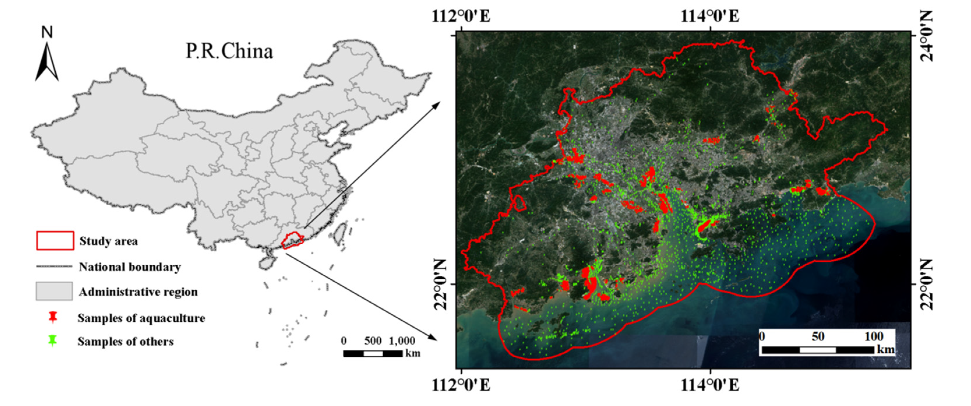
In this study, the Pearl River Basin (Guangdong) refers the part of the basin that located in Guangdong Province. The study area (Figure 1) covers the Pearl River Basin (Guangdong) and its 40 km buffer seaward from coastal line. The Pearl River with 2320 km long is the third-longest river in China, and it covers a region of subtropical maritime monsoon climate. The Pearl River Basin has been one of the most economically dynamic regions of China since ancient times. Local sea reclamation and marine aquaculture started very early, and especially the urbanization in the Pearl River Basin (Guangdong) is very fast since the launch of China’s Reform Programme in 1979. Currently, this specific region is one of the most developed regions in China; however, limited river networks cannot meet the demands of aquaculture developments [43]. Therefore, the expansions of aquaculture land are mainly concentrated in the ocean and coastal region. With years of developments, this region has become one of the biggest aquaculture bases with massive abundant inland aquaculture ponds and mariculture areas. The aquaculture, including fish farming, shrimp farming, oyster farming, mariculture, algaculture (such as seaweed farming) and the cultivation of ornamental fish, is well-developed in this region.

Figure 1.
Geographical locations of the Pearl River Basin (Guangdong) and study area (annual median images of sentinel-2A (2020) after cloud removal).
2.2. Data
Sentinel series satellites are the important branches of the Copernicus Programme satellite constellation conducted by the European Space Agency (ESA) and an essential part of Global Monitoring for Environment and Security (GMES). Sentinel-1 satellite constellation is the first of this specific program, and it carries C-band synthetic-aperture radar (SAR) instrument with a temporal resolution of 6 days [44]. The Sentinel-2A/B satellites equipped with Multispectral Instrument (MSI) are capable of acquiring high spatial resolution (up to 10 m) optical images in 13 spectral bands every 5 days [45]. The ESA and European Commission’s policies makes Sentinel’s data easily accessible [46]. More detailed technical specifications of both Sentinel-1 SAR and Sentinel-2A MSI data are available in previous studies [47,48] and will not be repeated here.
The standard Level-1 (ground range detected, GRD) data product of Sentinel-1 in Interferometric Wide Swath (IW) mode and the calibrated Bottom of Atmosphere (BOA) products of Sentienel-2 used in this study were offered by GEE. Considering the data availability, this study was only focused on 2020. One arc-minute global relief model of the Earth’s surface that integrates land topography and ocean bathymetry (ETOPO1) dataset was also collected to extract ocean bathymetry [49]. The Global Self-consistent, Hierarchical, High-resolution Geography Database (GSHHG) that comprises World Vector Shorelines (WVS) [50] was applied to extract shorelines of the study area. All these datasets were re-projected to the uniform coordinate reference system (WGS_1984_UTM_Zone_50N) and resampled to a same ground spatial resolution of 10 × 10 m.
3. Methods
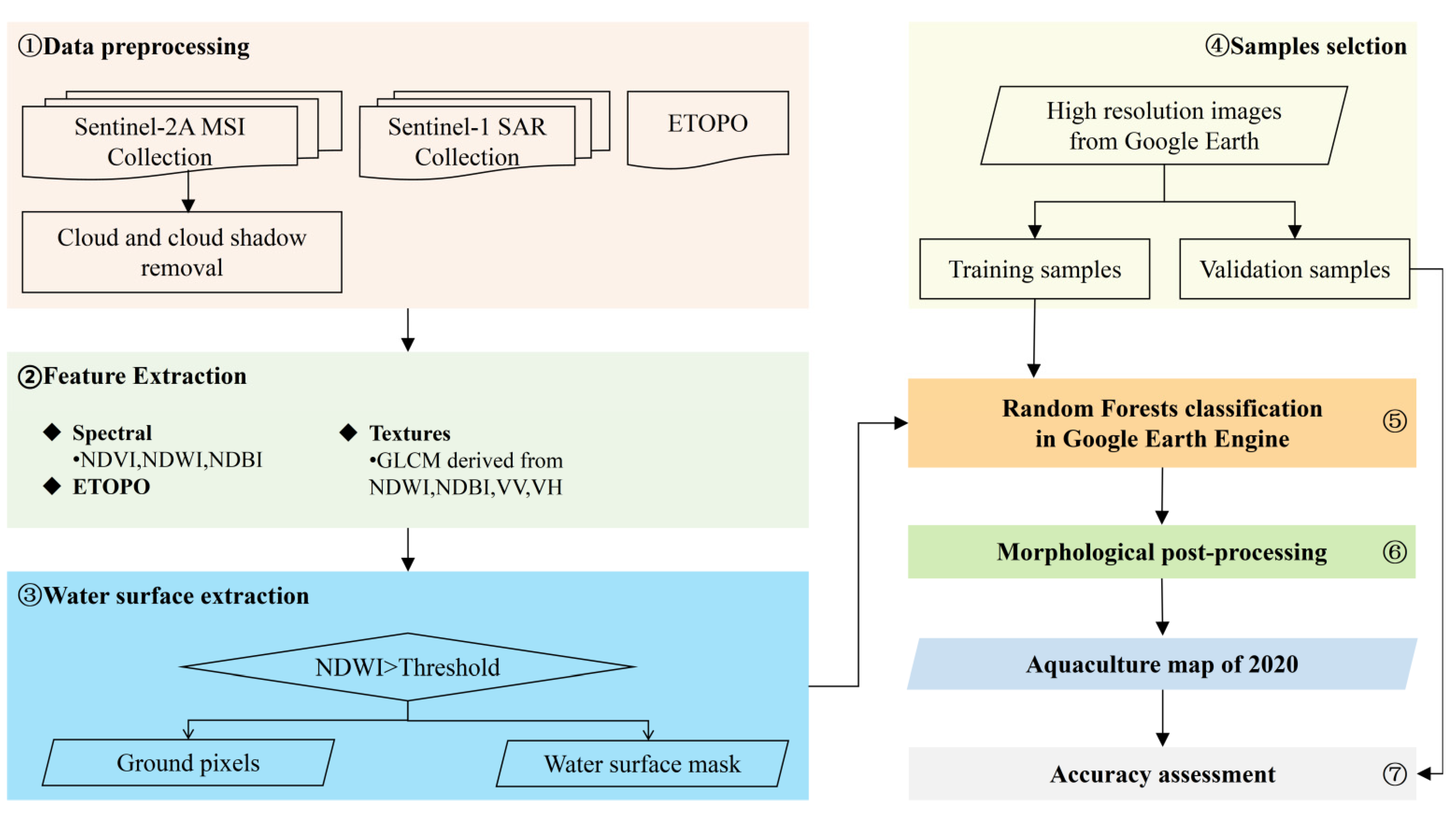
The approach proposed in this study for large-scale aquaculture mapping with multisource remotely sensed images and the GEE platform includes seven main steps (Figure 2): (1) data preprocessing, (2) feature extraction, (3) water surface extraction (including aquaculture land), (4) sample selection, (5) Random Forest classification in the GEE platform, (6) morphological post processing, and (7) accuracy assessment. These steps were repeated several times to find the optimal parameters.
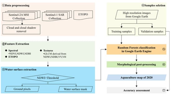
Figure 2.
Approach proposed in this study.
3.1. Data Preprocessing
A bitmask band with cloud mask information (QA60) for the Sentinel-2A image is provided on the GEE platform. Cloud and cloud shadow affecting observation quality were identified by the code based on the Function of Mask (CFMask) [51], and they were marked in the QA60 band. The clear-sky pixels were selected according to QA60, and the Sentinel-2A images in 2020 with less than 20% cloud and cloud shadow cover were used in this study.
3.2. Feature Extraction for Each Image Pixel
3.2.1. Image Features of Aquaculture Areas
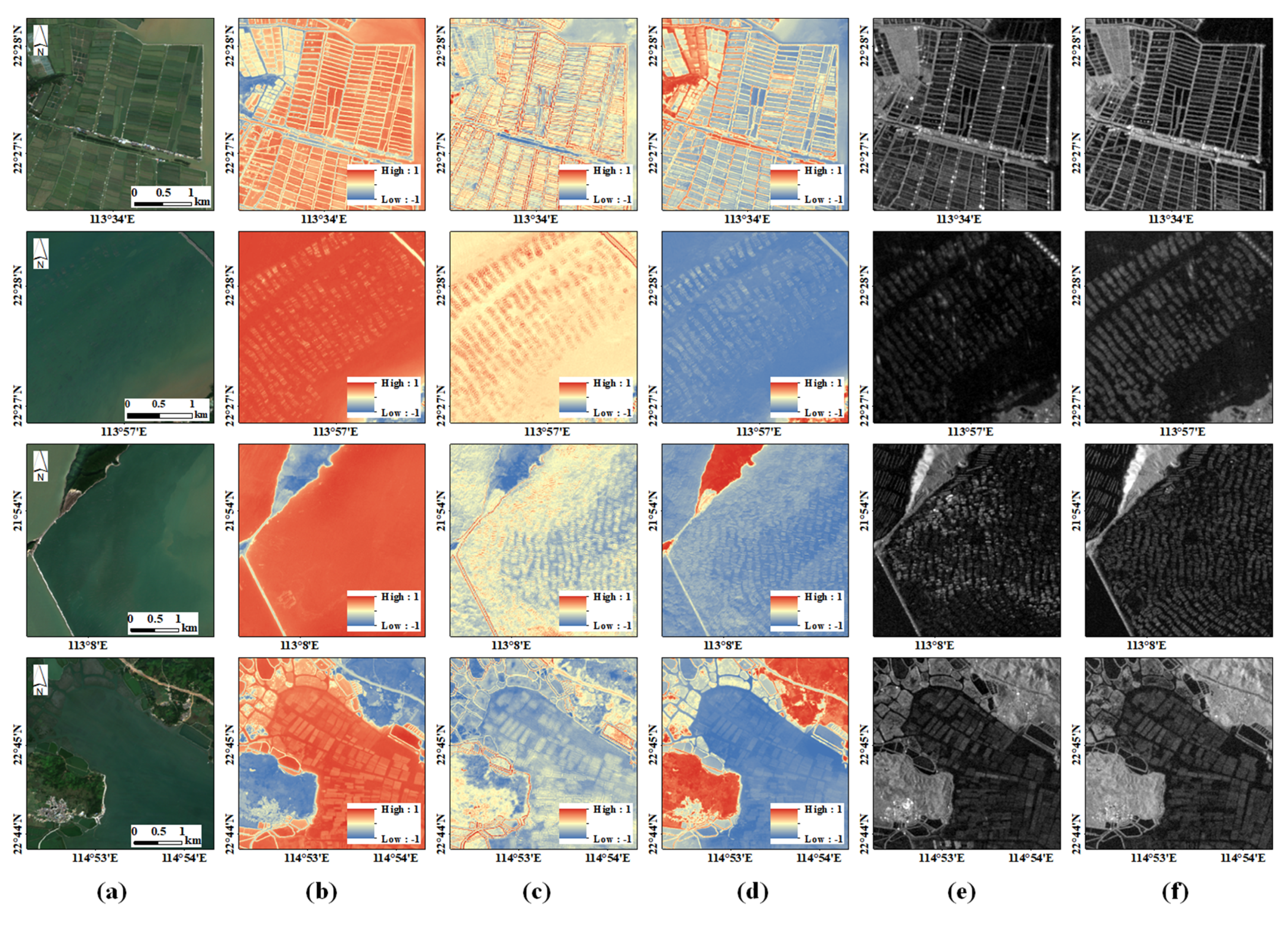
Only aquaculture ponds show regular shapes and textures on the Sentinel-2A multispectral images (Figure 3), because they are usually very large compared with medium-resolution image pixels. The spectral signatures of water ponds are also clearly presented in NDWI image, and texture features are clearly presented in all optical, spectral indices and SAR images.
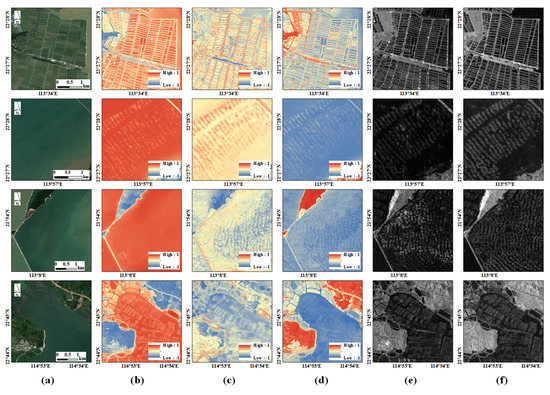
Figure 3.
Images and features of typical aquaculture areas: (a) Sentinel-2A multispectral image, (b) NDWI, (c) NDBI, (d) NDVI, (e) VV Polarization image, and (f) VH Polarization image.
Mariculture facilities do not show obvious signatures in Sentinel-2A multispectral optical images, because they are relatively small compared with medium-resolution image pixels, or some are submerged in water. However, these aquaculture types show significantly different characteristics in NDWI, NDVI and NDBI images, because normalized difference image features amplify the differences. More specifically, the textures are very clear in Sentinel-1 SAR images, because the backscatter signature of the radar is sensitive to the roughness and structure of water surface.
Based on the above analyses, we found that NDVI, NDWI, and NDBI could better highlight the differences between aquaculture areas and other water bodies and the textures derived from index images; VV and VH images could further enhance the differences.
3.2.2. Normalized Difference Spectral Indices
In this study, NDWI, NDVI [52] and NDBI [53] were used as spectral features.
Normalized Difference Water Index (NDWI) (Equation (1)): NDWI was proposed by McFeeters [54], based on the fact of strong spectral absorption of water body in the near-infrared (NIR) band, and it is a robust method for detecting aquaculture water surface and has proved effective in segmenting muddy aquaculture ponds [39]. Correspondingly, NDWI can be used to distinguish land and water bodies.
where ρgreen is the reflectance of green band (B3 of MSI), and ρnir represents the reflectance of near-infrared band (B8 of MSI).
In this study, the images with annual cloud cover less than 20% in 2020 were used to calculate a series of NDWI values. The NDWI series were sorted from small to large, and the 25% maximum NDWI values (located in the 75–100% of the sequence) were selected to calculate the average NDWI image. This preprocessing takes full use of all the image features for the whole year and eliminates the seasonal differences of aquaculture areas.
Normalized difference vegetation index (NDVI) (Equation (2)): Generally, aquaculture ponds usually have higher nutrients than natural water bodies, and the algae concentration is also higher. The waterbodies with high algae concentration generally have high reflectance in NIR spectrum compared with natural waters (without aquacultures). Therefore, NDVI may separate aquaculture waters from natural waters at a certain degree.
where ρred represents the reflectance of red band (B4 of MSI), and ρnir represents the reflectance of near-infrared band (B8 of MSI). Referring to the processing of NDWI, we also sorted and filtered the NDVI values (75–100%) to compose the final average NDVI image.
Normalized difference built-up index (NDBI) (Equation (3)): NDBI is originally designed to detect built-up and barren areas. In practice, the extracted water mask often contains shadow noise with low reflectivity, which may be caused by tall buildings over built-up areas. The surrounding pixels of shadows usually have high NDBI values, and thus it is able to distinguish building shadows by analyzing their surrounding pixels.
where ρswir1 represents the reflectance of the shortwave infrared band (B10 of MSI), and ρnir represents the reflectance of the near-infrared band (B8 of MSI). To further reduce the potential effects of shadow noise, we also sorted and filtered the NDBI values (75–100%) to compose the final average NDBI image. The morphological operation is an effective way to examine the neighbors of a pixel. Since a higher NDBI indicates a higher possibility of a built-up pixel, an inflation operator was conducted on the NDBI image to eliminate lathy and small building shadows, and a corrosion operator was further adopted to restore the image.
3.2.3. Backscatter Features
A single Sentinel-1 SAR image is usually contaminated by speckle noises, and previous studies demonstrated the effectiveness of SAR image enhancement using time series images [55]. Following Xia’s work [39], we selected the mean values of the VV and VH time series images of 75–100% in ascending order at the pixel level to form the final VV and VH image over the whole study area.
3.2.4. Texture Features
Image texture provides relevant characteristics of spatial structures. In this study, the aquaculture lands hold relative regular shapes and arrangements, which are reflected in the regular change of gray levels of images pixels. Considering the results of previous studies, we combined different kinds of textures to address the problem of insufficient accuracy and to reduce the interference of the surroundings.
Gray Level Co-occurrence Matrix (GLCM) [56] is a method to analyze texture characteristics, and it calculates the correlation between two gray levels to reflect the comprehensive information about directions, intervals, and the changes in magnitude and speed. Some studies suggested that better recognition performance could be obtained by using extreme values to calculate texture features in different directions than in any direction or average direction. NDWI, NDBI, and backscattering coefficient of VV/VH were employed as input images for calculating GLCM, with gray level of 16, 150 × 150 m sliding windows and four directions (Figure 4). The NDVI image was mainly used to distinguish aquaculture ponds and natural waters, and it was not applied to compute texture features in this study.

Figure 4.
Direction measure of GLCM calculation in this study.
Numerous texture feature bands (n = 18) can be generated using GLCM method in GEE. Redundant textural measures are possibly complex and may reduce computing speed, which may influence the performance of classification. Following Yu’s work [57], Angular Second Moment, Contrast, Correlation, Variance, Sum Average, Inverse Difference Moment, and Entropy were selected and computed from GLCM (Table 1), and their maximum and minimum values in four directions (Figure 4) were analyzed. Therefore, for each input image, a 14-dimension feature vector was obtained (7 measures × 2 values).

Table 1.
Textural measures based on GLCM method in this study.
3.3. Water Surface Extraction
The pixels with aquaculture areas mainly show pure water or water-dominated spectral responses, and the probability of water surface can be simply reflected by NDWI. Inspired by [39], the water surface was first detected from NDWI image by that a pixel with a NDWI value higher than a threshold was classified as water. The aquaculture facilities in the sea, rivers, or lakes show different spectral signatures from pure water bodies. The sizes of aquaculture facilities are relatively smaller than medium spatial resolution image pixels and some aquaculture facilities are submerged in the water, and thus the pixels with aquaculture facilities are mixed pixels. The NDWI values of pixels with aquaculture facilities are usually lower than those of pure water pixels but higher than those of other objects, and thus the mixed objects can be classified as water surface using a threshold.
3.4. Sample Selection
The aquaculture areas in the Pearl River Basin (Guangdong) hold regular spatial morphological characteristics in remotely sensed images (Figure 5). In this study, the aquaculture areas were roughly divided into inland aquaculture ponds and marine aquaculture. Inland aquaculture ponds are mainly distributed in the junction zone between water body (river, lake and sea) and land. The inland aquaculture ponds are formed through the reclamation of coastal wetlands or inland lakes, and they are usually partitioned by embankments and have regular and compact shapes (Figure 5b,c). Inland aquaculture pond units are usually clustered together, showing regular texture structures.
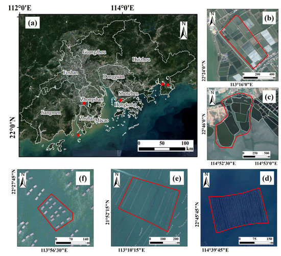
Figure 5.
Typical aquaculture samples over the study area in high resolution Google Earth image (a): costal aquaculture pond (b,c), visible raft aquaculture (d,e), and concentrated-distributed cage culture area (f).
Marine aquaculture areas are often located in bays and inshore seawaters, and they include raft aquaculture (Figure 5d,e) and cage aquaculture (Figure 5f). The raft aquaculture facilities in neritic zone are composed of aquatic bamboo raft (for floating) and subaquatic thick rope (for fixing aquatic products). Correspondingly, the raft aquaculture areas are characterized by dull grey stripes (Figure 5d,e). The cage culture areas consist of aquatic plastic frames and suspended net cages (Figure 5f). Comparing with water bodies, cage aquaculture facilities appear as brighter colors in remotely sensed imagery, and their distributions are more concentrated, with regular rectangles.
In this study, a total number of 8317 samples were selected for classifier training (n = 7317) (Table 2) and accuracy assessment (n = 1000).

Table 2.
Classification system used in this study.
3.5. Random Forest (RF) Classification on GEE Platform
GEE provides a serial of classification algorithms, including Minimum Distance (MD) [58], Random Forest (RF) [59], Support Vector Machine (SVM) [60], Regression Trees (CART) [61] and Naive Bayes (NB) [62]. According to previous studies, SVM and RF have better performance than other classification algorithms [63,64,65]. SVM algorithm performs good with limited training samples, however, RF performs better as training sets get larger [66]. RF is conceptually similar to tree-based learners, and they share same advantages [67]. RF can exhibit higher accuracy and efficiency even facing the unfavorable conditions of noise interference. Moreover, RF classifier shows better performance than other classifiers in land cover mapping using long time series images [68,69]. Therefore, RF classifier was employed in this study.
In this study, the composed NDVI, NDWI and NDBI products were also employed as spectral attributes of each pixel, the GLCM features of NDWI, NDBI, VV and VH were used as texture attributes, and the ETOPO1 value was applied as a topographic attribute. A feature vector of 60 dimensions (3 spectral + 4 images × 14 measures/image texture + 1 topographic) was obtained. A RF classifier on GEE platform was trained according to existing reference [70], in which the number of trees (ntree) was set to 100, the maximum depth was unlimited, the minimum sample number of each tree node was 1, and the number of features for each tree was set as the square root of the variable number.
3.6. Morphological Post Processing
Based on the above process, the aquaculture areas in the Pearl River Basin (Guangdong) were obtained preliminarily. However, the texture difference between aquaculture land and streamway were not clearly detected, which may cause misclassification. Streamway is one of the equipped facilities of aquaculture ponds. The obvious morphological difference between open water and streamway can be observed, and thus the compactness of each extracted aquaculture pond was calculated for modifying misclassification with Equation (4), which reflects the geometric shape of the object. The threshold of compactness was set as 11.5 through a trial-and-error process.
where W and H are the width and height of the minimum enclosing rectangle, respectively, and Area is the number of inner pixels of the object. The small holes (≤1000 pixels) within aquaculture patches were filled, and the isolated small patches (≤3 pixels) were removed. An illustration of post processes is presented in Figure 6.

Figure 6.
Overview of the morphological post processes of extracted aquaculture land in this study: (a) raw classification results based on RF, (b) exclusion of misclassified river, and (c) final classification map with postprocessing.
3.7. Accuracy Assessment
A total of 1000 samples of aquacultures extracted from Google Earth images using visual interpretation were used as ground-truth references. The confusion matrix was first obtained, and then overall accuracy and Kappa coefficient were applied to assess the accuracy of the proposed approach.
3.8. Optimal Parameter Selection
Several key factors affect the final classification performance: feature combination, window size to compute textures and threshold to extract water surface. The steps described in Section 3.1, Section 3.2, Section 3.3, Section 3.4, Section 3.5, Section 3.6 and Section 3.7 were repeated, and the values of these key factors maximizing overall accuracy were selected.
Feature Combination: Based on different types of features, including normalized difference spectral indices, backscatter features and image textures derived from spectral indices and SAR images, many kinds of feature combinations can be obtained. To investigate the optimal feature combination, six groups of features (Table 3) were used to obtain six aquaculture maps, respectively. The threshold T = 0.06 and texture window size with 15 were used. The determinations of T and window size are described in Section 4.2 and Section 4.3, respectively. The 1000 random selected samples were used to evaluate their performances.

Table 3.
Classification performances using different feature combinations.
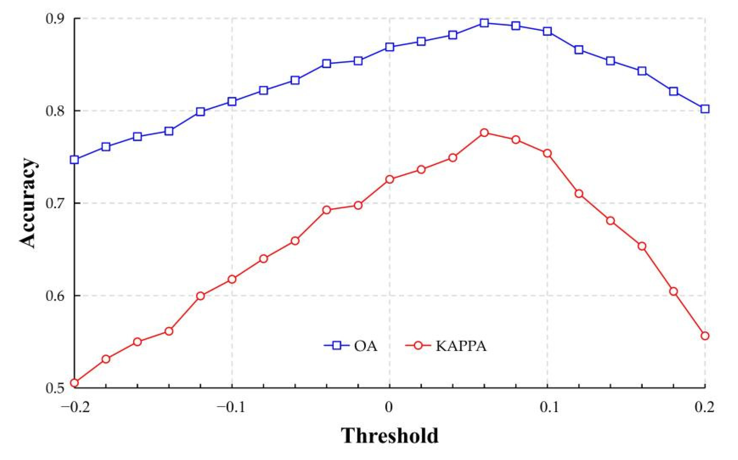
Threshold to Extract Water Surface: Since aquaculture areas are first classified as a part of a water body, the threshold separating water and non-water surfaces plays an important role in the whole process. In this study, water surface was extracted by thresholding an NDWI image, and only one parameter T was used. The spectral indices, textures from indices and SAR images, as well as ETOPO1, were used. The window size was set at 15 × 15 pixels. The thresholds between −0.2 and 0.2 were tested, with a step of 0.02. The accuracies were evaluated using 1000 samples.
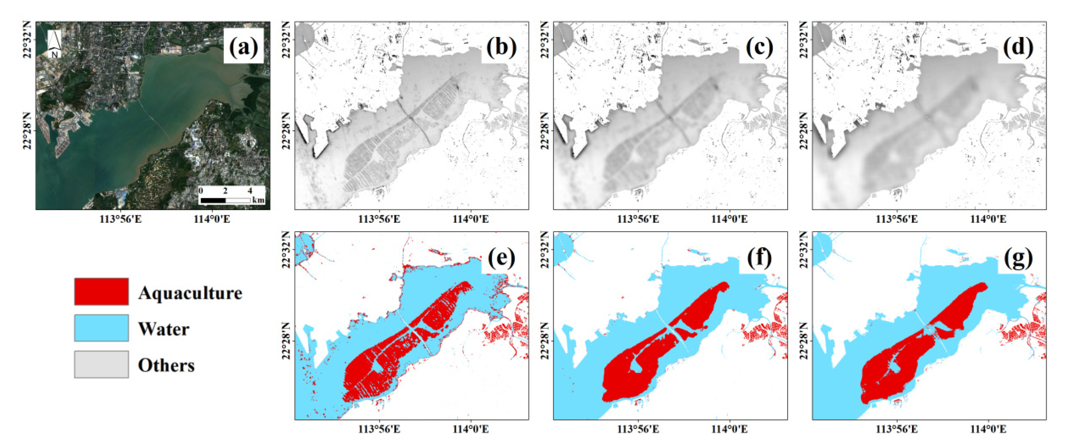
Window Size to Compute GLCM Features: The window size of gray-level co-occurrence matrix can directly affect the detection of aquaculture in a complex water environment. According to [71], a texture window should cover at least the minimum detectable target. Although inland aquaculture ponds have regular arrangements and clear textures, the ponds can be properly separated by thresholding NDWI image. However, the detection of mariculture facilities mainly depends on image textures. Based on our visual interpretation from Google Earth, the size of minimum detectable mariculture block is about 50 to 150 m. Therefore, a window size of 15 × 15 pixels was preferred. However, the experiments using a window of 5 × 5 pixels, 15 × 15 pixels, and 30 × 30 pixels were also carried out to determine the optimal size.
4. Results
4.1. Aquaculture Maps Obtained Using Multiple Features
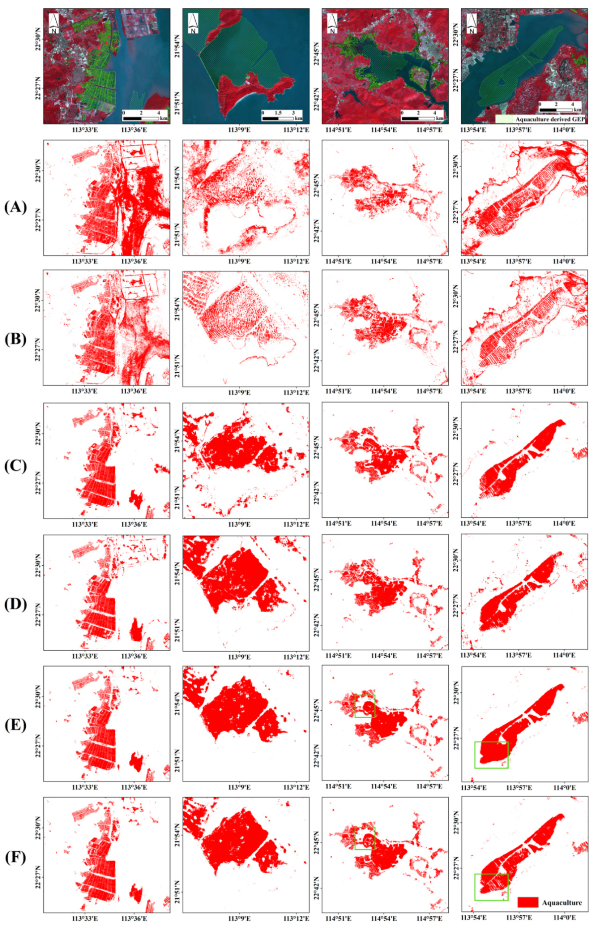
Six maps were obtained using different feature combinations; their accuracies were assessed with 1000 validation samples (Table 3), and four typical sites of the maps were presented in Figure 7. The performances using only spectral indices were poor (Figure 7A and Table 3), and many water pixels were wrongly classified as aquaculture pixels, for some aquaculture facilities are submerged in waters and their spectral signatures are not obliviously different from water. The combination of spectral indices and SAR image features improved the performance (Figure 7B), especially for the second typical site, for SAR images reflect the backscatter characteristics of aquaculture facilities, which is totally different from a pure water body. However, many misclassifications still existed near shorelines, and the overall accuracy and Kappa coefficient are not satisfactory. The use of spectral indices and index-derived texture features greatly improved the classification performance (Figure 7C and Table 3), and most aquaculture ponds and mariculture areas were correctly detected, and an overall accuracy of 88.2% was obtained.
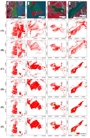
Figure 7.
Aquaculture maps obtained using different feature combinations. The first-row present images and reference aquaculture areas at four typical sites, and the results of combinations (A–F) are presented in the second to seventh rows. The details of feature combinations are presented in Table 3.
The results of combination D (Figure 7D) show the effectiveness of using SAR images and their corresponding textures. Comparing the results on the second site with those from combination C, it can be easily found that mariculture areas were better detected. However, there are many commission errors along coastlines, resulting in a lower OA (86.9%). The results in Figure 7 show that the combination of E and F obtained better performances than the combination of A, B, C, and D. However, the results of combination E had less holes, and the overall accuracy (89.5%) and Kappa coefficient (0.719) were both the highest compared with other combinations. Therefore, the feature in combination E was applied to obtain the final map.
4.2. Optimal Threshold for Water Body Segmentation
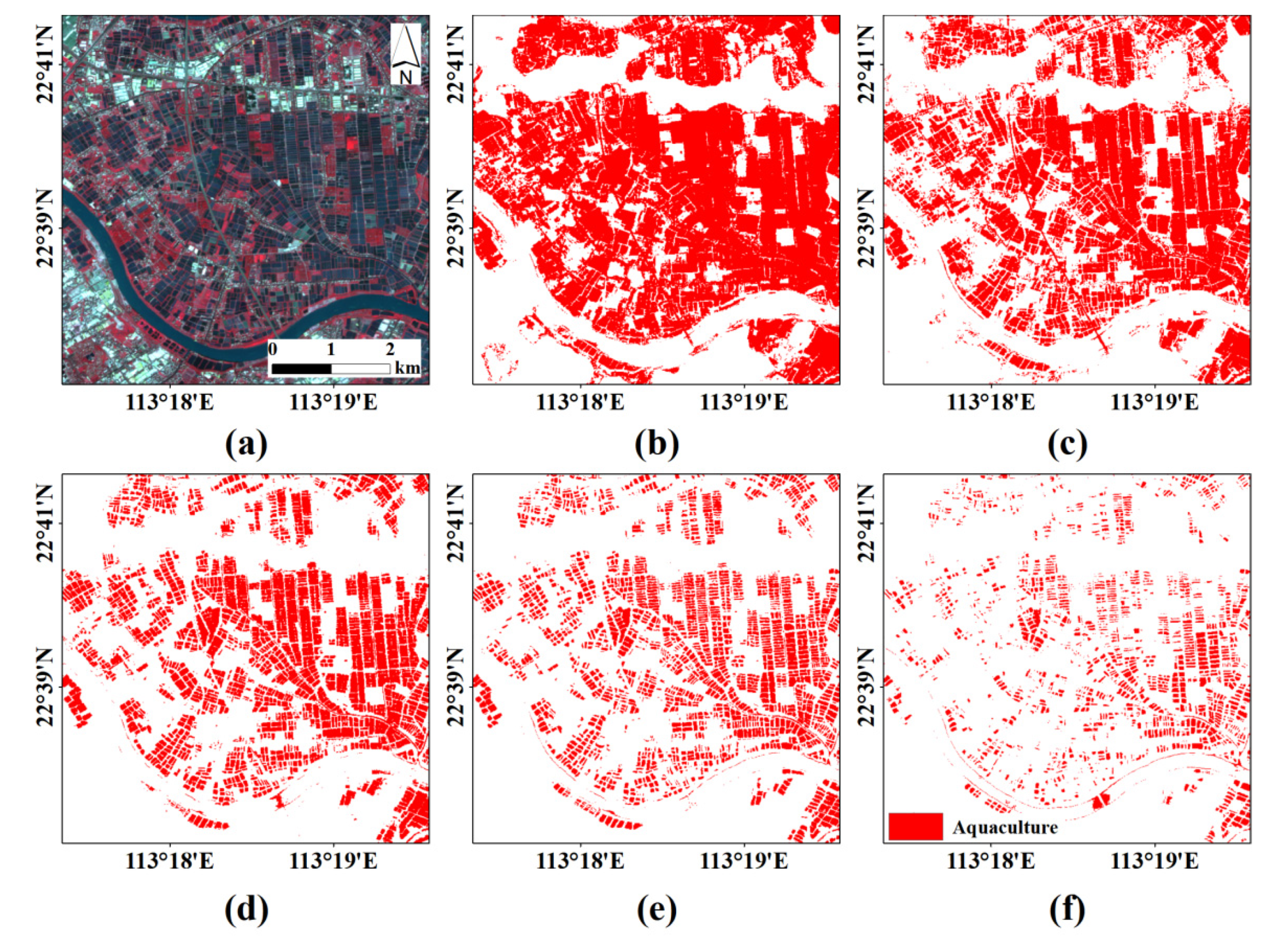
A total of 21 aquaculture maps were obtained using thresholds from −0.2 to 0.2; their overall accuracies and Kappa coefficients are presented in Figure 8, and five maps over a typical area are presented in Figure 9.
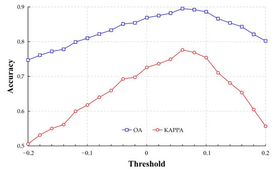
Figure 8.
Overall accuracies and Kappa coefficients using different thresholds.

Figure 9.
Typical classification maps using different thresholds: (a) Sentinel-2A MSI image, (b) T = −0.2, (c) T = −0.1, (d) T = 0, (e) T = 0.1, and (f) T = 0.2.
The overall accuracy and Kappa coefficient were low with a very small threshold (T = −0.2), due to many misclassified land pixels. With a small threshold, many mixed pixels containing waters were segmented as water surface, and further classified as aquaculture areas. As shown in Figure 9b, many embankment pixels were wrongly segmented as water surface and further misclassified as aquaculture areas. As the threshold increased, the misclassifications were gradually overcome (Figure 9b–d), the overall accuracy gradually increased, and finally the overall accuracy achieved the best result with T = 0.06. As the threshold further increased, the accuracy decreased for many mixed pixels and even some pure water pixels were segmented as land, and thus many aquaculture ponds were missed (Figure 9f). Generally, the optimal threshold is a balance of the two misclassification types, and the threshold 0.06 was preferred in our study.
4.3. Optimal Window Size for Texture Calculation
Figure 10 shows the maximum sum averaged texture derived from VH and the extracted aquaculture with a window size of 5 × 5 pixels, 15 × 15 pixels, and 30 × 30 pixels, respectively. Some small misclassifications were observed along shorelines with the window size of 5 × 5 pixels. With 15 × 15 windows, the textures better delineated the existing aquaculture areas, resulting in a satisfactory result (Figure 10f). With larger window size (30 × 30 pixels), the texture feature was over-smoothed. Moreover, the computational load dramatically increased with the increase in window size. Therefore, the window size of 15 × 15 pixels was used in this study.

Figure 10.
Maximum sum average texture of VH using different window sizes and the aquaculture maps: (a) Sentinel-2A false color images, (b–d) image features with a window size of 5 × 5 pixels, 15 × 15 pixels and 30 × 30 pixels, and (e–g) aquaculture maps.
4.4. Aquaculture Map and Accuracy Assessment
With optimal feature combination, threshold, and window size, the final aquaculture maps were obtained (Figure 11). The aquacultures in the Pearl River Basin (Guangdong) had a total area of 1445.91 km2 in 2020. The inland aquacultures were concentrated in the coast of bays, including Zhenhai Bay (Figure 11a), Yamen watercourse (Figure 11b), Pearl River Estuary (Figure 11g) and Niwanmen watercourse (Figure 11h). The area along the coast had the most concentrated aquacultures, which are mainly enclosed sea aquacultures. Moreover, a great deal of inland aquacultures were widely distributed in the inland river network.
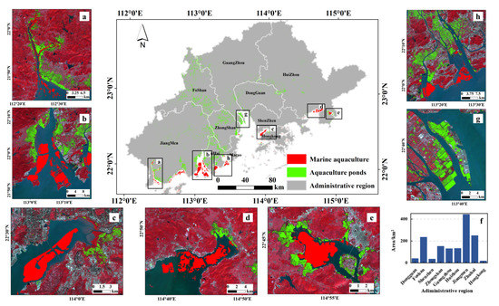
Figure 11.
Aquaculture maps in the Pearl River Basin (Guangdong) in 2020: (a) Zhenhai Bay, (b)Yamen watercourse, (c) Shenzhen Bay, (d) Baisha Bay, (e) Baisha lake, (f) Histogram of aquaculture area in major administrative regions, (g) Pearl River Estuary, and (h) Niwanmen watercourse.
Marine aquacultures accounted for 22.8% of the total area of aquaculture in the Pearl River Basin (Guangdong), and they were concentrated in the bays along the coast. The raft cultures were mainly distributed in Yamen watercourse (Figure 11b) and Baisha Bay (Figure 11d), and cage culture in Shenzhen Bay (Figure 11d) and and Baisha lake (Figure 11e). The aquaculture areas of the major administrative regions in the Pearl River Basin (Guangdong) in 2020 are shown in Figure 11h. Jiangmen City had the largest area of aquaculture with about 443.56 km2, which accounts for about 30.7% of the total aquaculture area in the study area. The second was Zhuhai City, with an aquaculture area of 251.52 km2, accounting for 17.4% of the total aquaculture area.
The validation of aquaculture area map with the validation samples held an overall accuracy of 89.5% with a kappa coefficient of 0.776, a Producer’s Accuracy of 82.82%, and a User’s Accuracy of 89.47% (Table 4). Some commission and omissions errors for the proposed approach were still observed. Using a window of 150 × 150 m, some water bodies and tidal flats adjacent to aquaculture were misclassified as aquaculture because of their similar edge texture values. In addition, the aquacultures with high sediment content have similar spectral characteristics with non-aqueous bodies, and they were frequently misclassified.

Table 4.
Confusion matrix of proposed approach using 1000 validation samples.
The high user’s and overall accuracies indicated the satisfactory performance of the proposed approach. However, the producer’s accuracy was slightly lower than user’s accuracy, for some mixed pixels containing parts of ponds were classified as water bodies at the stage of NDWI thresholding. This problem could be overcome by using sub-pixel mapping or high spatial resolution images.
5. Discussion
5.1. Comparison with Other Aquaculture Maps
The proposed approach in this study was compared with the methods proposed by Duan et al. [42] and Xia et al. [39]. The corresponding reference images were manually labeled. The maps are presented in Figure 12, and the confusion matrixes are presented in Table 5, Table 6 and Table 7. Duan et al. [42] adopted a spectrum, and spatial and morphological features of 30 m resolution Landsat images to build a Random Forest classifier to implement an automatic extraction of large-scale aquacultures. Xia’s et al. [39] extracted the water surface from Sentinel-2A images using multiple thresholds, described the water patches using geometric and spectral features, and finally applied a Random Forest classifier to classify inland aquaculture ponds.
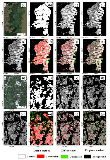
Figure 12.
Aquaculture maps obtained using three methods. (a,i) present the Sentinel-2A true color images, and their corresponding reference maps are presented in (e,m). The results obtained using Duan’s [42], Xia’s [39], and the proposed approach are presented in (b–d) and (j–l), respectively. Their comparisons with the ground truth maps are presented in (f–h) and (n–p), respectively.

Table 5.
Confusion matrix of Duan’s method in typical sites [42].

Table 6.
Confusion matrix of Xia’s method in typical sites [39].

Table 7.
Confusion matrix of proposed approach in this study in typical sites.
The map provided by Duan et al. [42] presented a general distribution of aquaculture ponds; however, almost all the details were missed (Figure 12b,j), for it was obtained using Landsat TM images with a spatial resolution of 30 m. Moreover, they conducted morphological closing and erosion operations post process, which further smoothed the details.
Xia’s method and the proposed approach in this study were applied to two typical regions, and their derived aquaculture maps were compared. Xia’s [39] and the proposed approach in this study produced similar aquaculture maps, and most of their details are clearer than Duan’s map (Figure 12c,d,k,l) for Sentinel images of 10 m spatial resolution were applied and the post processing did not eliminate the details. The proposed method produced similar results to Xia’s method (Figure 12c,d,k,l); however, less embankment pixels were misclassified. Therefore, the User’s Accuracy of aquaculture areas (92.40%) was higher than that of Xia’s method (77.97%). The main problem of the proposed method is that some isolated ponds were missed, resulting in a lower Producer’s Accuracy (Table 7). However, the overall accuracy and Kappa coefficient indicated that the proposed method performed better over the tested areas.
The proposed approach in this study achieved better performance than Duan’s and Xia’s methods, which might be explained by that: (1) the texture features from normalized difference spectral index images increased the distinguishability of aquaculture area from other objects; and (2) radar images were integrated with optical ones, as they are sensitive to the texture structure of aquaculture areas, resulting in further improvement for aquaculture mapping. More important, the proposed approach was originally designed to simultaneously map aquaculture ponds and mariculture areas, whereas Xia’s and Duan’s methods can only map aquaculture ponds, and thus the proposed method has a better generalizability.
5.2. Impacts of Mixed-Pixels
The aquaculture maps in the Pear River Basin (Guangdong) were obtained with medium resolution Sentinel-1 SAR and Sentinel-2A multispectral images, and the results showed the advantages of using medium resolution images for large-scale thematic mapping. However, the accuracy and generalization of the proposed approach might be affected by mixed pixels of medium resolution images. The aquaculture pixels are often mixed with embankment among ponds, which often results in ambiguous boundaries and some inevitable errors. Thus, some parts of aquaculture ponds were classified as land, and some embankments were classified as ponds. It is difficult to overcome such errors using medium spatial resolution images, and very high spatial resolution images may easily overcome this problem.
The step of extracting water surface mask in our proposed approach is also affected by mixed pixels. Our method relies on the assumption that pixels covering mariculture facilities are still water-dominated, because the sizes of these facilities are usually relatively smaller than a pixel. Thus, they were first classified as waterbodies, and further been detected at later stages. However, this assumption may be not appropriate when using high spatial resolution images, because many pixels covering mariculture facilities are no longer water-dominated mixed pixels. In such case, these pixels will be segmented into non-aquaculture, affecting the accuracy of final map. Object-based methods might be an optimal solution for high spatial resolution images to overcome this limitation.
The proposed approach was designed for large scale aquaculture mapping using medium spatial resolution images. Although the boundaries are not detected very accurately, the aquaculture map over a large area can be efficiently obtained. In particularly, the medium spatial resolution images acquired by many satellite sensors (such as Landsat TM series and Sentinel-2A series) for several decades provide great convenience to monitor the development of the aquaculture industry.
5.3. Selection of Time Series Images
In this study, time series images for a whole year were used for aquaculture mapping in order to eliminate the influence of accidental factors, such as water-dominated paddy fields and dry ponds during harvest period. Time series SAR images also are effective in suppressing speckle noise of radar image. Although there are many advantages, two problems should be noted.
First, the seasonal characteristics of study areas may affect the selection of time series images. For example, this study area is located in southern China, in which the temperature is usually high, and the water does not freeze; thus, the images with good quality acquired at any time can be used. However, in northern China, the pond water freezes in winter and its optical properties will change. Therefore, the time series images should be selected according to the specific seasonal characteristics of study areas.
Second, the assumption and basis of using time series images are that ground entities are not changed suddenly. If some aquaculture ponds are converted into agricultural land or built-up areas in winter, they may still be recognized as aquaculture areas. To improve the ability to respond to such sudden changes, it is necessary to shorten the time interval of time series images.
5.4. Limits and Future Works
An effective and efficient approach was proposed in this study for aquaculture area mapping over large areas; however, some issues should be further investigated. Firstly, some narrow rivers adjacent to aquaculture ponds were still misclassified. Thus, more accurate classifier and post-processing methods are still worth investigating, and the combination of post-processing and river vector boundaries may be a potential solution. Secondly, the aquaculture areas were roughly classified into two types in this study: aquaculture ponds and mariculture areas, and more specific aquaculture types are needed to be investigated. Finally, only one global threshold was used to extract waterbodies (containing aquaculture areas); it was not always optimal for different and complex image scenes, and thus a locally adaptive thresholding approach is a potential solution to improve the segmentation of the water surface. Only the aquaculture maps in 2020 were obtained in this study, and they are not sufficient for more potential applications. With historic earth observation images, it is necessary to analyze the long-time spatial–temporal changes of aquaculture areas and their impacts on economy and ecological systems and further to provide supports for the sustainable developments of the study area.
6. Conclusions
A novel approach was proposed in this study for simultaneously mapping multi-type aquaculture areas over large scale areas by combining spectral and texture features from optical (Sentinel-2A multispectral) and radar (Sentinel-1) images, and a case study in the Pear l River Basin (Guangdong) showed its efficiency. The main contribution of this work could be summarized as follows:
(1) We analyzed the spectral and textural features of aquaculture areas and demonstrated the effectiveness of fusing multiple image features for aquaculture mapping. We found that the use of textural features derived from the spectral indices can greatly improve the mapping accuracy and the use of textural features derived from SAR images can further improve mapping accuracy, as they are sensitive to marine aquaculture facilities.
(2) The proposed approach could generate a more accurate aquaculture map than previous studies. Moreover, the proposed approach was implemented on the GEE platform, and has great potential for national-scale and long-term aquaculture mapping.
Author Contributions
Conceptualization, Z.H.; methodology, Z.H., Y.X.; validation, Y.X., Y.Y.; formal analysis, Z.H., Y.X., J.W. and Y.Z.; investigation, Y.X. and Y.Y.; data curation, Y.X. and Y.Y.; writing—original draft preparation, Y.X. and Z.H.; writing—review and editing, Z.H., J.W., Y.Z. and G.W.; visualization, Y.X.; supervision, Z.H.; project administration, Z.H.; funding acquisition, Z.H. All authors have read and agreed to the published version of the manuscript.
Funding
This work was jointly supported by the National Natural Science Foundation of China (NSFC) (No. 41871227), the Natural Science Foundation of Guangdong Province (No. 2020A1515010678, 2020A1515111142) and the Basic Research Program of Shenzhen (No. JCYJ20190808122405692, 20200812112628001).
Institutional Review Board Statement
Not applicable.
Informed Consent Statement
Not applicable.
Data Availability Statement
The codes and data are available from this linkage: https://github.com/XuBenBen15045812917/Muilti-aquaculture_extraction.git (accessed on 25 October 2021).
Acknowledgments
We thank Xia at Eastern China Normal University for providing their code and Duan at Jiangsu Normal University for providing their aquaculture map for comparison.
Conflicts of Interest
The authors declare no conflict of interest.
References
- Ottinger, M.; Clauss, K.; Kuenzer, C. Aquaculture: Relevance, distribution, impacts and spatial assessments—A review. Ocean. Coast. Manag. 2016, 119, 244–266. [Google Scholar] [CrossRef]
- Cao, L.; Naylor, R.; Henriksson, P.; Leadbitter, D.; Metian, M.; Troell, M.; Zhang, W.B. China’s aquaculture and the world’s wild fisheries. Science 2015, 347, 133–135. [Google Scholar] [CrossRef] [PubMed]
- FAO. The State of World Fisheries and Aquaculture 2018-Meeting the Sustainable Development Goals; FAO: Rome, Italy, 2018; pp. 1–227. [Google Scholar]
- Pauly, D.; Zeller, D. Agreeing with FAO: Comments on SOFIA 2018. Mar. Policy 2019, 100, 332–333. [Google Scholar] [CrossRef]
- Wang, Q.; Cheng, L.; Liu, J.; Li, Z.; Xie, S.; De Silva, S.S. Freshwater aquaculture in PR China: Trends and prospects. Rev. Aquac. 2015, 7, 283–302. [Google Scholar] [CrossRef]
- Cao, L.; Wang, W.; Yang, Y.; Yang, C.; Yuan, Z.; Xiong, S.; Diana, J. Environmental impact of aquaculture and countermeasures to aquaculture pollution in China. Environ. Sci. Pollut. Res. 2007, 14, 452–462. [Google Scholar] [CrossRef]
- Moffitt, C.M.; Cajas-Cano, L. Blue Growth: The 2014 FAO State of World Fisheries and Aquaculture. Fisheries 2014, 39, 552–553. [Google Scholar] [CrossRef]
- Pham, T.D.; Yokoya, N.; Bui, D.T.; Yoshino, K.; Friess, D.A. Remote Sensing Approaches for Monitoring Mangrove Species, Structure, and Biomass: Opportunities and Challenges. Remote Sens. 2019, 11, 230. [Google Scholar] [CrossRef]
- Alexandridis, T.K.; Topaloglou, C.A.; Lazaridou, E.; Zalidis, G.C. The performance of satellite images in mapping aquacultures. Ocean. Coast. Manag. 2008, 51, 638–644. [Google Scholar] [CrossRef]
- Jayanthi, M.; Rekha, P.N.; Kavitha, N.; Ravichandran, P. Assessment of impact of aquaculture on Kolleru Lake (India) using remote sensing and Geographical Information System. Aquac. Res. 2006, 37, 1617–1626. [Google Scholar] [CrossRef]
- Virdis, S.G.P. An object-based image analysis approach for aquaculture ponds precise mapping and monitoring: A case study of Tam Giang-Cau Hai Lagoon, Vietnam. Environ. Monit. Assess. 2014, 186, 117–133. [Google Scholar] [CrossRef]
- Ottinger, M.; Clauss, K.; Kuenzer, C. Large-Scale Assessment of Coastal Aquaculture Ponds with Sentinel-1 Time Series Data. Remote Sens. 2017, 9, 440. [Google Scholar] [CrossRef]
- Wang, M.; Cui, Q.; Wang, J.; Ming, D.P.; Lv, G.N. Raft cultivation area extraction from high resolution remote sensing imagery by fusing multi-scale region-line primitive association features. ISPRS J. Photogramm. Remote Sens. 2017, 123, 104–113. [Google Scholar] [CrossRef]
- Ottinger, M.; Clauss, K.; Kuenzer, C. Opportunities and Challenges for the Estimation of Aquaculture Production Based on Earth Observation Data. Remote Sens. 2018, 10, 1076. [Google Scholar] [CrossRef]
- Liu, Y.; Wang, Z.; Yang, X.; Zhang, Y.; Yang, F.; Liu, B.; Cai, P. Satellite-based monitoring and statistics for raft and cage aquaculture in China’s offshore waters. Int. J. Appl. Earth Obs. Geoinf. 2020, 91, 102118. [Google Scholar] [CrossRef]
- Aguilar-Manjarrez, J.; Travaglia, C. Mapping Coastal Aquaculture and Fisheries Structures by Satellite Imaging Radar: Case Study of the Lingayen Gulf, the Philippines; Food Agriculture Organization: Roma, Italy, 2004. [Google Scholar] [CrossRef]
- Ren, C.; Wang, Z.; Zhang, B.; Li, L.; Chen, L.; Song, K.; Jia, M. Remote Monitoring of Expansion of Aquaculture Ponds Along Coastal Region of the Yellow River Delta from 1983 to 2015. Chin. Geogr. Sci. 2018, 28, 430–442. [Google Scholar] [CrossRef]
- Xing, Q.; An, D.; Zheng, X.; Wei, Z.; Wang, X.; Li, L.; Tian, L.; Chen, J. Monitoring seaweed aquaculture in the Yellow Sea with multiple sensors for managing the disaster of macroalgal blooms. Remote Sens. Environ. 2019, 231, 111279. [Google Scholar] [CrossRef]
- Sakamoto, T.; Van Phung, C.; Kotera, A.; Nguyen, K.D.; Yokozawa, M. Analysis of rapid expansion of inland aquaculture and triple rice-cropping areas in a coastal area of the Vietnamese Mekong Delta using MODIS time-series imagery. Landsc. Urban Plan. 2009, 92, 34–46. [Google Scholar] [CrossRef]
- Liu, Y.; Yang, X.; Wang, Z.; Lu, C.; Li, Z.; Yang, F. Aquaculture area extraction and vulnerability assessment in Sanduao based on richer convolutional features network model. J. Oceanol. Limnol. 2019, 37, 1941–1954. [Google Scholar] [CrossRef]
- Cui, B.; Fei, D.; Shao, G.; Lu, Y.; Chu, J. Extracting Raft Aquaculture Areas from Remote Sensing Images via an Improved U-Net with a PSE Structure. Remote Sens. 2019, 11, 2053. [Google Scholar] [CrossRef]
- Zhang, T.; Yang, X.M.; Hu, S.S.; Su, F.Z. Extraction of coastline in aquaculture coast from multispectral remote sensing images: Object-based region growing integrating edge detection. Remote Sens. 2013, 5, 4470–4487. [Google Scholar] [CrossRef]
- Zhang, T.; Li, Q.; Yang, X.; Zhou, C.; Su, F. Automatic Mapping Aquaculture in Coastal Zone from TM Imagery with OBIA Approach. In Proceedings of the 2010 18th International Conference on Geoinformatics, Beijing, China, 18–20 June 2010; pp. 1–4. [Google Scholar] [CrossRef]
- Zeng, Z.; Wang, D.; Tan, W.; Huang, J. Extracting aquaculture ponds from natural water surfaces around inland lakes on medium resolution multispectral images. Int. J. Appl. Earth Obs. Geoinf. 2019, 80, 13–25. [Google Scholar] [CrossRef]
- Wang, J.; Sui, L.; Yang, X.; Wang, Z.; Liu, Y.; Kang, J.; Lu, C.; Yang, F.; Liu, B. Extracting Coastal Raft Aquaculture Data from Landsat 8 OLI Imagery. Sensors 2019, 19, 1221. [Google Scholar] [CrossRef] [PubMed]
- Komatsu, T.; Takahashi, M.; Ishida, K.; Suzuki, T.; Hiraishi, T.; Tameishi, H. Mapping of aquaculture facilities in Yamada Bay in Sanriku Coast, Japan, by IKONOS satellite imagery. Fish. Sci. 2002, 68, 584–587. [Google Scholar] [CrossRef][Green Version]
- Fan, J.; Zhao, J.; An, W.; Hu, Y. Marine Floating Raft Aquaculture Detection of GF-3 PolSAR Images Based on Col-lective Multikernel Fuzzy Clustering. IEEE J. Sel. Top. Appl. Earth Obs. Remote Sens. 2019, 12, 2741–2754. [Google Scholar] [CrossRef]
- Ren, C.; Wang, Z.; Zhang, Y.; Zhang, B.; Chen, L.; Xi, Y.; Xiao, X.; Doughty, R.; Liu, M.; Jia, M.; et al. Rapid expansion of coastal aquaculture ponds in China from Landsat observations during 1984–2016. Int. J. Appl. Earth Obs. Geoinf. 2019, 82, 101902. [Google Scholar] [CrossRef]
- Hu, Y.; Fan, J.; Wang, J. Target Recognition of Floating Raft Aquaculture in SAR Image Based on Statistical Region Merging. In Proceedings of the 2017 Seventh International Conference on Information Science and Technology (ICIST), Da Nang, Vietnam, 16–19 April 2017; pp. 429–432. [Google Scholar] [CrossRef]
- Zhang, Y.; Wang, C.; Ji, Y.; Chen, J.; Deng, Y.; Chen, J.; Jie, Y. Combining Segmentation Network and Nonsubsampled Contourlet Transform for Automatic Marine Raft Aquaculture Area Extraction from Sentinel-1 Images. Remote Sens. 2020, 12, 4182. [Google Scholar] [CrossRef]
- Prasad, K.A.; Ottinger, M.; Wei, C.; Leinenkugel, P. Assessment of Coastal Aquaculture for India from Sentinel-1 SAR Time Series. Remote Sens. 2019, 11, 357. [Google Scholar] [CrossRef]
- Zhang, K.; Dong, X.; Liu, Z.; Gao, W.; Hu, Z.; Wu, G. Mapping Tidal Flats with Landsat 8 Images and Google Earth Engine: A Case Study of the China’s Eastern Coastal Zone circa 2015. Remote Sens. 2019, 11, 924. [Google Scholar] [CrossRef]
- Jia, M.; Wang, Z.; Mao, D.; Ren, C.; Wang, C.; Wang, Y. Rapid, robust, and automated mapping of tidal flats in China using time series Sentinel-2 images and Google Earth Engine. Remote Sens. Environ. 2021, 255, 112285. [Google Scholar] [CrossRef]
- Halder, B.; Bandyopadhyay, J. Vegetation scenario of Indian part of Ganga Delta: A change analysis using Sentinel-1 time series data on Google earth engine platform. Saf. Extreme Environ. 2021, 1–14. [Google Scholar] [CrossRef]
- Th, A.; Emt, A.; Gang, C.B.; Gang, S.C.; Yz, D.; Yang, L.A.; Kz, A.; Yf, A. Mapping fine-scale human disturbances in a working landscape with Landsat time series on Google Earth Engine. ISPRS J. Photogramm. Remote Sens. 2021, 176, 250–261. [Google Scholar]
- Gorelick, N.; Hancher, M.; Dixon, M.; Ilyushchenko, S.; Thau, D.; Moore, R. Google Earth Engine: Planetary-scale geospatial analysis for everyone. Remote Sens. Environ. 2017, 202, 18–27. [Google Scholar] [CrossRef]
- Wang, C.; Liu, H.-Y.; Zhang, Y.; Li, Y.-F. Classification of land-cover types in muddy tidal flat wetlands using remote sensing data. J. Appl. Remote Sens. 2014, 7, 073457. [Google Scholar] [CrossRef]
- Tieng, T.; Sharma, S.; Mackenzie, R.A.; Venkattappa, M.; Sasaki, N.K.; Collin, A. Mapping mangrove forest cover using Landsat-8 imagery, Sentinel-2, Very High Resolution Images and Google Earth Engine algorithm for entire Cambodia. IOP Conf. Ser. Earth Environ. Sci. 2019, 266, 012010. [Google Scholar] [CrossRef]
- Xia, Z.; Guo, X.; Chen, R. Automatic extraction of aquaculture ponds based on Google Earth Engine. Ocean. Coast. Manag. 2020, 198, 105348. [Google Scholar] [CrossRef]
- Sun, Z.; Luo, J.; Yang, J.; Yu, Q.; Zhang, L.; Xue, K.; Lu, L. Nation-Scale Mapping of Coastal Aquaculture Ponds with Sentinel-1 SAR Data Using Google Earth Engine. Remote Sens. 2020, 12, 3086. [Google Scholar] [CrossRef]
- Duan, Y.; Li, X.; Zhang, L.; Chen, D.; Liu, S.; Ji, H. Mapping national-scale aquaculture ponds based on the Google Earth Engine in the Chinese coastal zone. Aquaculture 2020, 520, 734666. [Google Scholar] [CrossRef]
- Duan, Y.; Tian, B.; Li, X.; Liu, D.; Sengupta, D.; Wang, Y.; Peng, Y. Tracking changes in aquaculture ponds on the China coast using 30 years of Landsat images. Int. J. Appl. Earth Obs. Geoinf. 2021, 102, 102383. [Google Scholar] [CrossRef]
- Richards, R.; Ruddle, K.; Zhong, G. Integrated agriculture-aquaculture in South China: The dike-pond System of the Zhujiang Delta. Geogr. Rev. 1989, 79, 260–262. [Google Scholar] [CrossRef]
- Snoeij, P.; Torres, R.; Geudtner, D.; Brown, M.; Deghaye, P.; Navastraver, I.; Ostergaard, A.; Rommen, B.; Floury, N.; Da-vidson, M. Sentinel-1 Instrument Overview; Esa Special Publication: Noordwijk, The Netherlands, 1 March 2013; pp. 2–5. [Google Scholar]
- Martimort, P.; Fernandez, V.; Kirschner, V.; Isola, C.; Meygret, A. Sentinel-1 Multispectral Imager(MSI) and Calibration/Validation. In Proceedings of the IEEE International Geoscience and Remote Sensing Symposium (IGARSS), Munich, Germany, 22–27 July 2012; pp. 6999–7002. [Google Scholar]
- Main-Knorn, M.; Pflug, B.; Louis, J.; Debaecker, V.; Müller-Wilm, U.; Gascon, F. Sen2Cor for Sentinel-2. In Proceedings of the Conference on Image and Signal Processing for Remote Sensing, Warsaw, Poland, 4 October 2017; p. 3. [Google Scholar] [CrossRef]
- Li, Y.; Niu, Z.; Xu, Z.; Yan, X. Construction of High Spatial-Temporal Water Body Dataset in China Based on Sentinel-1 Archives and GEE. Remote Sens. 2020, 12, 2413. [Google Scholar] [CrossRef]
- Sibanda, M.; Buthelezi, S.; Ndlovu, H.S.; Mothapo, M.C.; Mutanga, O. Mapping the Eucalyptus spp woodlots in communal areas of Southern Africa using Sentinel-2 Multi-Spectral Imager data for hydrological applications. Phys. Chem. Earth 2021, 122, 102999. [Google Scholar] [CrossRef]
- Center, N. Hypsographic Curve of Earth’s Surface from ETOPO1. Available online: Ngdc.noaa.gov (accessed on 26 October 2021).
- Wessel, P.; Smith, W.H.F. A global, self-consistent, hierarchical, high-resolution shoreline database. J. Geophys. Res. Solid Earth 1996, 101, 8741–8743. [Google Scholar] [CrossRef]
- Zhu, Z.; Wang, S.; Woodcock, C.E. Improvement and expansion of the Fmask algorithm: Cloud, cloud shadow, and snow detection for Landsats 4–7, 8, and Sentinel 2 images. Remote Sens. Environ. 2015, 159, 269–277. [Google Scholar] [CrossRef]
- Pettorelli, N. Using the satellite-derived NDVI to assess ecological responses to environmental change. Trends Ecol. Evol. 2005, 20, 503–510. [Google Scholar] [CrossRef]
- Osgouei, P.E.; Kaya, S.; Sertel, E.; Alganci, U. Separating built-up Areas from bare land in Mediterranean cities using Sentinel-2A imagery. Remote Sens. 2019, 11, 345. [Google Scholar] [CrossRef]
- McFeeters, S.K. The use of the Normalized Difference Water Index (NDWI) in the delineation of open water features. Int. J. Remote Sens. 1996, 17, 1425–1432. [Google Scholar] [CrossRef]
- Liew, S.C.; Kam, S.P.; Chen, P.; Muchlisin, Z.A. Mapping Tsunami-Affected Coastal Aquaculture Areas in Northern Sumatra Using High Resolution Satellite Imagery. In Proceedings of the Asian Association on Remote Sensing—26th Asian Conference on Remote Sensing and 2nd Asian Space Conference, Hanoi, Vietnam, 7–11 November 2005; pp. 116–120. [Google Scholar]
- Haralick, R.M.; Shanmugam, K.; Dinstein, I. Textural Features for Image Classification. IEEE Trans. Syst. Man Cybern. 1973, SMC-3, 610–621. [Google Scholar] [CrossRef]
- Yu, G.; Zhou, X.; Hou, D.; Wei, D. Abnormal crowdsourced data detection using remote sensing image features. Int. Arch. Photogramm. Remote Sens. Spat. Inf. Sci. 2021, 215–221. [Google Scholar] [CrossRef]
- Hodgson, M.E. Reducing the computational requirements of the minimum-distance classifier. Remote Sens. Environ. 1988, 25, 117–128. [Google Scholar] [CrossRef]
- Belgiu, M.; Drăguţ, L. Random forest in remote sensing: A review of applications and future directions. ISPRS J. Photogramm. Remote Sens. 2016, 114, 24–31. [Google Scholar] [CrossRef]
- Halldorsson, G.H.; Benediktsson, J.A.; Sveinsson, J.R. Support Vector Machines in Multisource Classification. In Proceedings of the 23rd International Geoscience and Remote Sensing Symposium (IGARSS 2003), Toulouse, France, 21–25 July 2003; pp. 2054–2056. [Google Scholar]
- Manno, A. CART: Classification and regression trees. Int. J. Public Health 2012, 57, 243–246. [Google Scholar]
- Yang, B.; Yu, X. Remote Sensing Image Classification of Geoeye-1 High-Resolution Satellite. ISPRS Int. Arch. Photogramm. Remote Sens. Spat. Inf. Sci. 2014, XL-4, 325–328. [Google Scholar] [CrossRef]
- Clemente, J.P.; Fontanelli, G.; Ovando, G.G.; Roa, Y.L.B.; Lapini, A.; Santi, E. Google Earth Engine: Application of Algorithms for Remote Sensing of Crops in Tuscany (ITALY). In Proceedings of the IEEE Latin American GRSS and ISPRS Remote Sensing Conference (LAGIRS), Santiago, Chile, 21–26 March 2020; pp. 195–200. [Google Scholar]
- Chung, L.C.H.; Xie, J.; Ren, C. Improved machine-learning mapping of local climate zones in metropolitan areas using composite Earth observation data in Google Earth Engine. Build. Environ. 2021, 199, 107879. [Google Scholar] [CrossRef]
- Shaharum, N.S.N.; Shafri, H.Z.M.; Ghani, W.A.W.A.K.; Samsatli, S.; Al-Habshi, M.M.A.; Yusuf, B. Oil palm mapping over Peninsular Malaysia using Google Earth Engine and machine learning algorithms. Remote Sens. Appl. Soc. Environ. 2020, 17, 100287. [Google Scholar] [CrossRef]
- Piragnolo, M.; Masiero, A.; Pirotti, F. Comparison of Random Forest and Support Vector Machine Classifiers Using UAV Remote Sensing Imagery. In Proceedings of the 19th Egu General Assembly Conference, Vienna, Austria, 23–28 April 2017; p. 15692. [Google Scholar]
- Cutler, D.R.; Edwards, T.C.E., Jr.; Beard, K.H.; Cutler, A.; Hess, K.T.; Gibson, J.; Lawler, J.J. Random Forests for Classification in Ecology. Ecology 2007, 88, 2783–2792. [Google Scholar] [CrossRef] [PubMed]
- Zhou, B.; Okin, G.S.; Zhang, J. Leveraging Google Earth Engine (GEE) and machine learning algorithms to incorporate in situ measurement from different times for rangelands monitoring. Remote Sens. Environ. 2020, 236, 111521. [Google Scholar] [CrossRef]
- Pelletier, C.; Valero, S.; Inglada, J.; Champion, N.; Dedieu, G. Assessing the robustness of Random Forests to map land cover with high resolution satellite image time series over large areas. Remote Sens. Environ. 2016, 187, 156–168. [Google Scholar] [CrossRef]
- Phan, T.N.; Kuch, V.; Lehnert, L. Land Cover Classification using Google Earth Engine and Random Forest Classifier—The Role of Image Composition. Remote Sens. 2020, 12, 2411. [Google Scholar] [CrossRef]
- Pesaresi, M.; Gerhardinger, A.; Kayitakire, F. A robust built-up area presence index by anisotropic rotation-invariant textural measure. J. Sel. Top. Appl. Earth Obs. Remote Sens. 2008, 1, 180–192. [Google Scholar] [CrossRef]
Publisher’s Note: MDPI stays neutral with regard to jurisdictional claims in published maps and institutional affiliations. |
© 2021 by the authors. Licensee MDPI, Basel, Switzerland. This article is an open access article distributed under the terms and conditions of the Creative Commons Attribution (CC BY) license (https://creativecommons.org/licenses/by/4.0/).

