
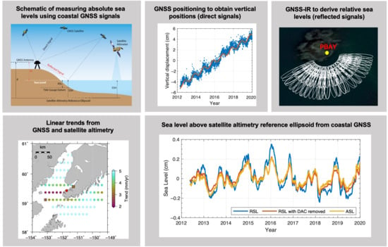
Measuring Coastal Absolute Sea-Level Changes Using GNSS Interferometric Reflectometry


Abstract
:
1. Introduction
2. Data and Methods
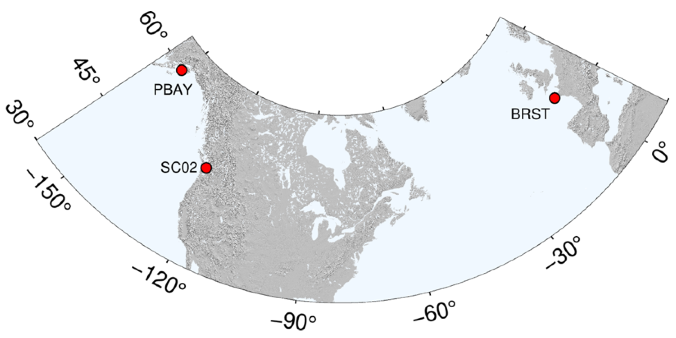
2.1. Data
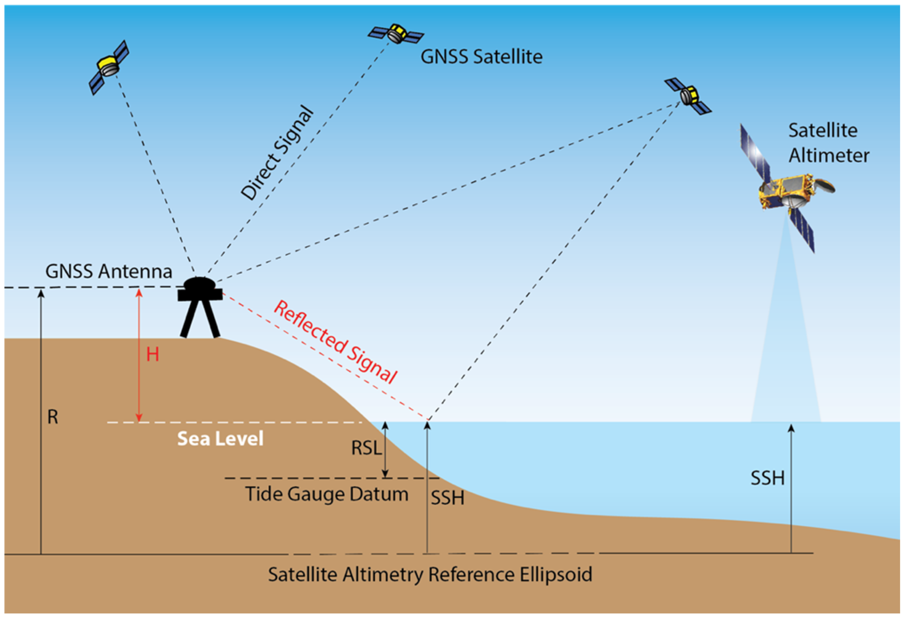
2.2. SSH from Satellite Altimetry and Coastal GNSS Stations
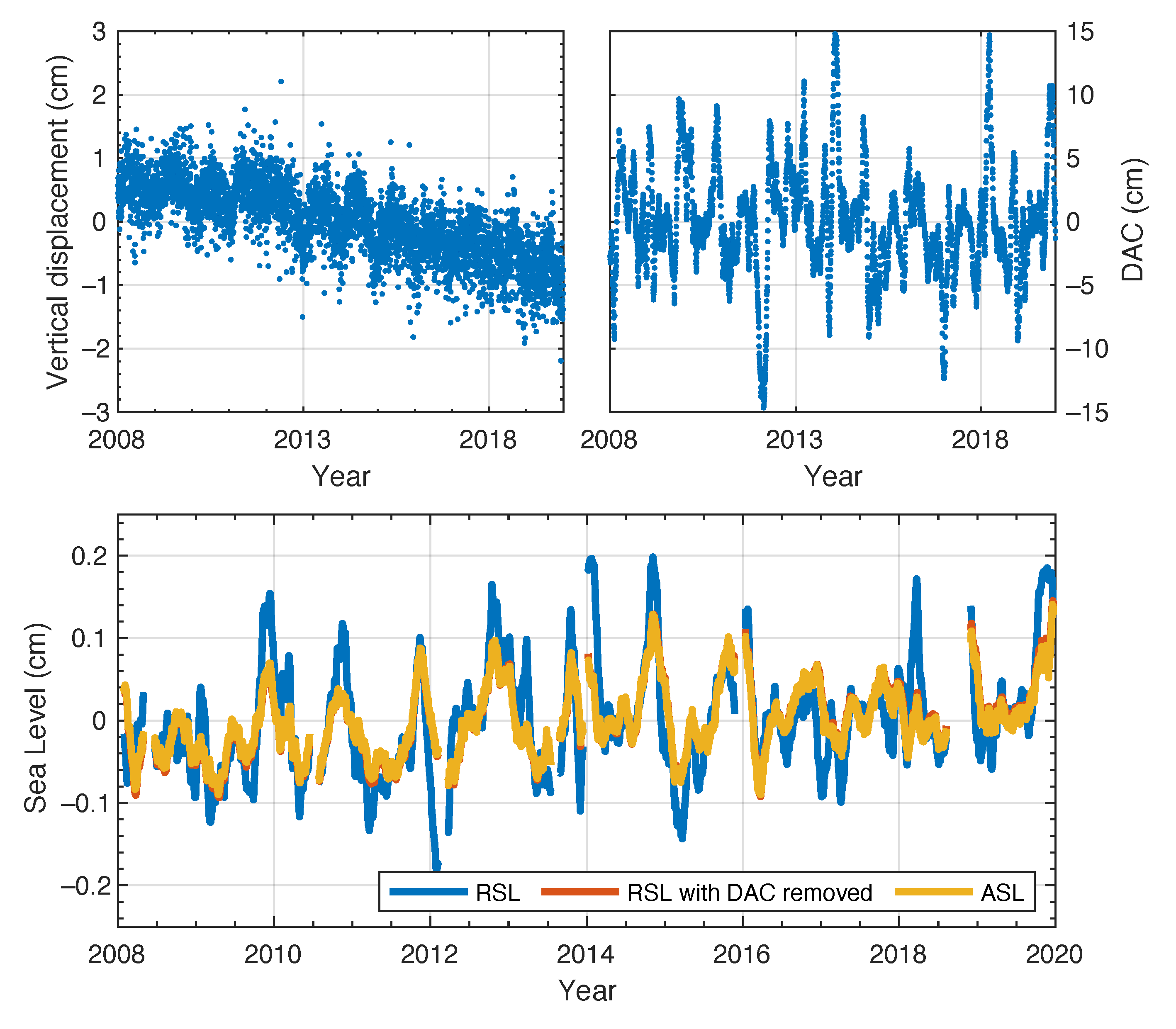
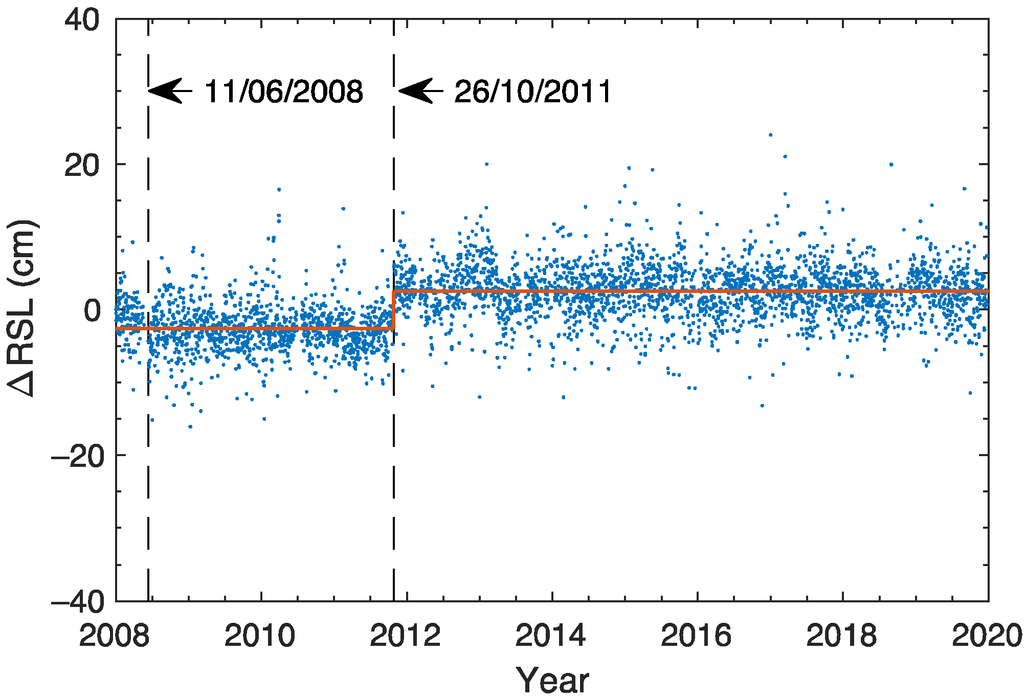
2.3. Artificial Offset Caused by Change of GNSS Equipment
3. Results
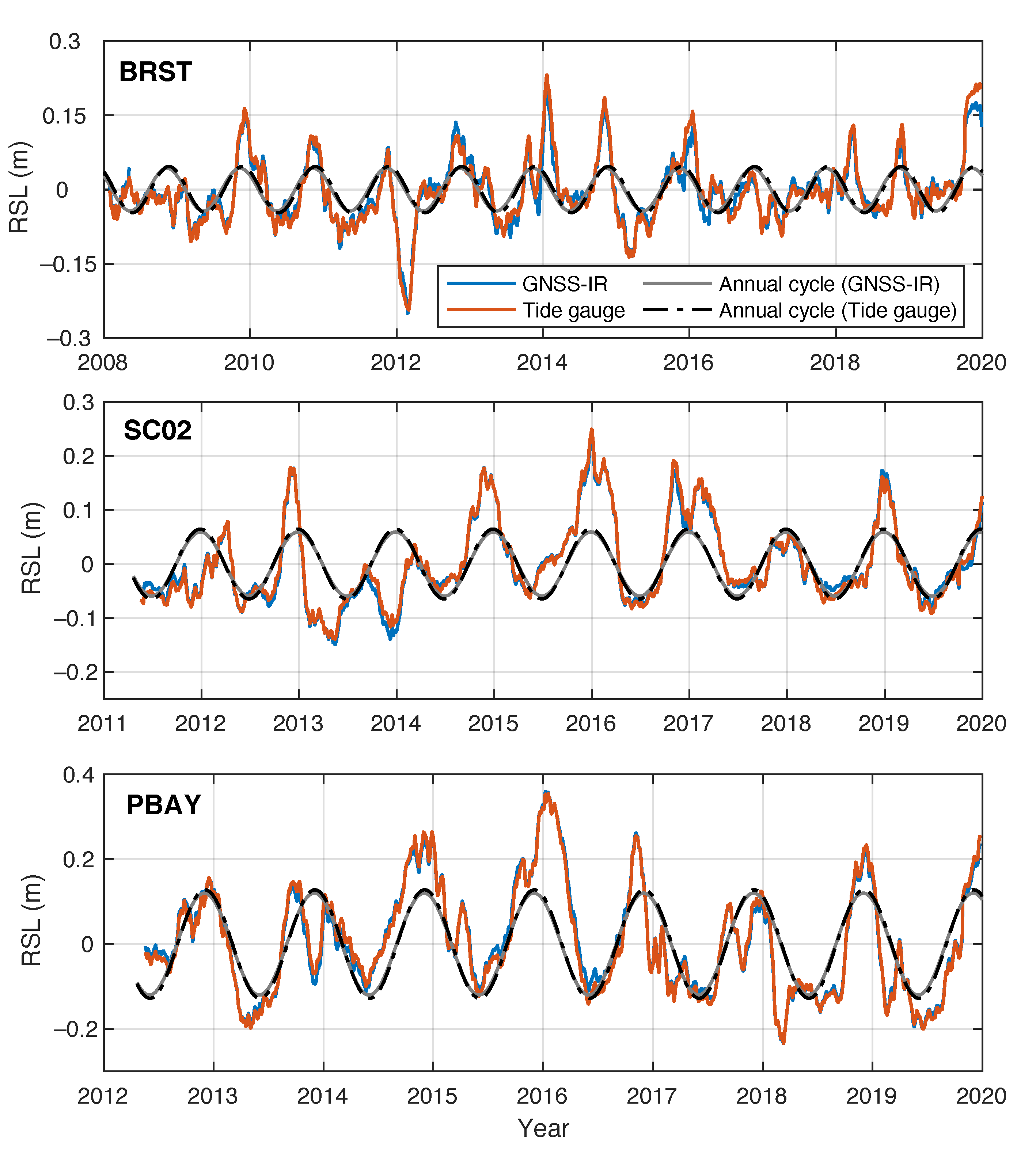
3.1. Relative Sea-Level Changes from GNSS-IR and Tide Gauges
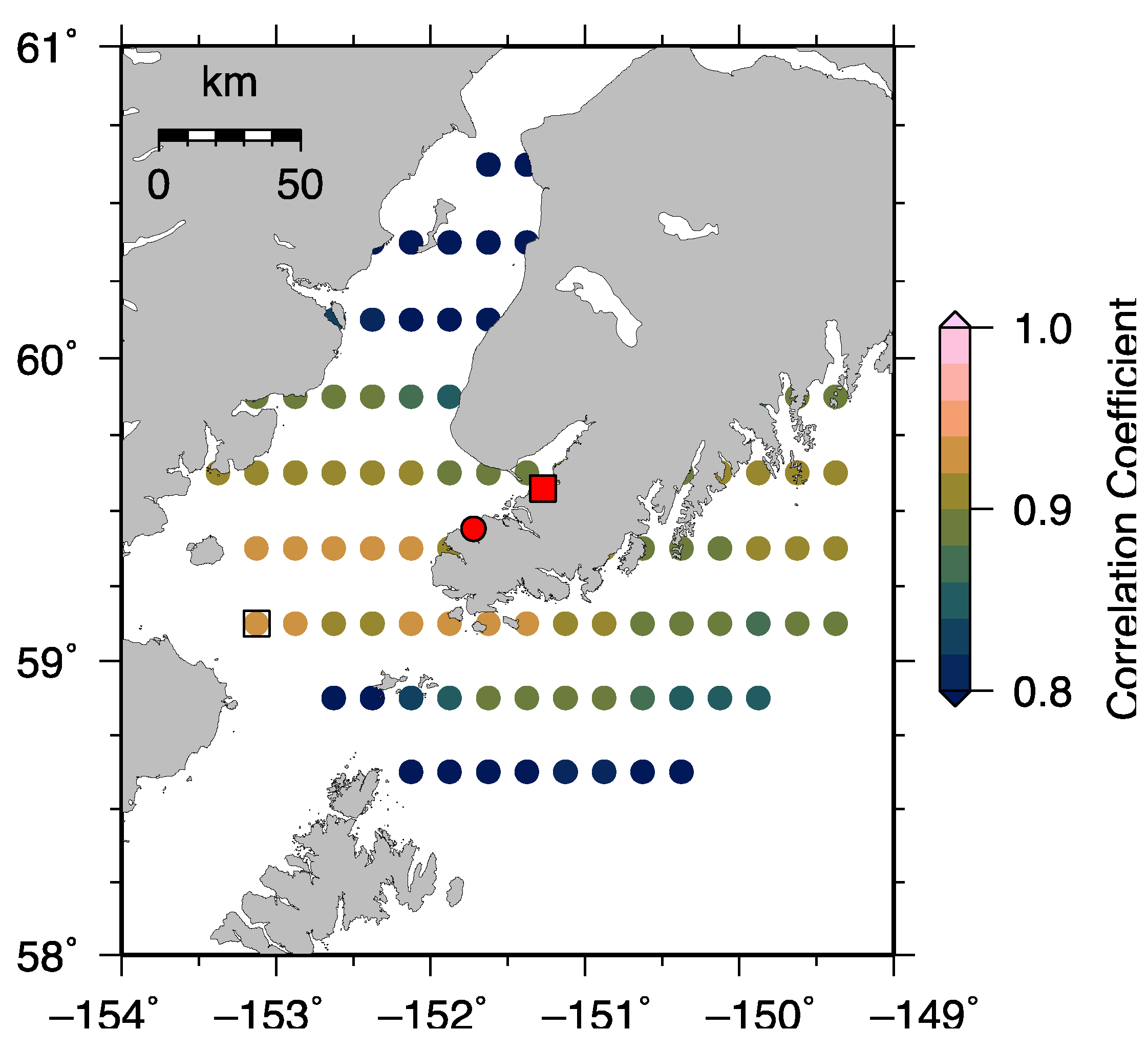
3.2. Absolute Sea-Level Changes from GNSS-IR and Satellite Altimetry
4. Discussion
5. Conclusions
Author Contributions
Funding
Data Availability Statement
Acknowledgments
Conflicts of Interest
Appendix A


References
- Li, L.; Switzer, A.D.; Wang, Y.; Chan, C.-H.; Qiu, Q.; Weiss, R. A modest 0.5-m rise in sea level will double the tsunami hazard in Macau. Sci. Adv. 2018, 4, eaat1180. [Google Scholar] [CrossRef] [PubMed] [Green Version]
- Kulp, S.A.; Strauss, B.H. New elevation data triple estimates of global vulnerability to sea-level rise and coastal flooding. Nat. Commun. 2019, 10, 1–12. [Google Scholar]
- Befus, K.; Barnard, P.L.; Hoover, D.J.; Hart, J.F.; Voss, C.I. Increasing threat of coastal groundwater hazards from sea-level rise in California. Nat. Clim. Chang. 2020, 10, 946–952. [Google Scholar] [CrossRef]
- Pokhrel, Y.; Felfelani, F.; Satoh, Y.; Boulange, J.; Burek, P.; Gädeke, A.; Gerten, D.; Gosling, S.N.; Grillakis, M.; Gudmundsson, L. Global terrestrial water storage and drought severity under climate change. Nat. Clim. Chang. 2021, 11, 226–233. [Google Scholar] [CrossRef]
- Benveniste, J.; Cazenave, A.; Vignudelli, S.; Fenoglio-Marc, L.; Shah, R.; Almar, R.; Andersen, O.; Birol, F.; Bonnefond, P.; Bouffard, J.; et al. Requirements for a Coastal Hazards Observing System. Front. Mar. Sci. 2019, 6. [Google Scholar] [CrossRef] [Green Version]
- Pugh, D.; Woodworth, P. Sea-Level Science: Understanding Tides, Surges, Tsunamis and Mean Sea-Level Changes; Cambridge University Press: Cambridge, UK, 2014. [Google Scholar]
- Fu, L.L.; Christensen, E.J.; Yamarone, C.A.; Lefebvre, M.; Menard, Y.; Dorrer, M.; Escudier, P. TOPEX/POSEIDON mission overview. J. Geophys. Res. Ocean. 1994, 99, 24369–24381. [Google Scholar] [CrossRef]
- Wöppelmann, G.; Marcos, M. Vertical land motion as a key to understanding sea level change and variability. Rev. Geophys. 2016, 54, 64–92. [Google Scholar] [CrossRef] [Green Version]
- Santamaría-Gómez, A.; Gravelle, M.; Collilieux, X.; Guichard, M.; Míguez, B.M.; Tiphaneau, P.; Wöppelmann, G. Mitigating the effects of vertical land motion in tide gauge records using a state-of-the-art GPS velocity field. Glob. Planet. Chang. 2012, 98, 6–17. [Google Scholar] [CrossRef]
- Cipollini, P.; Calafat, F.M.; Jevrejeva, S.; Melet, A.; Prandi, P. Monitoring sea level in the coastal zone with satellite altimetry and tide gauges. In Integrative Study of the Mean Sea Level and Its Components; Springer: Berlin/Heidelberg, Germany, 2017; pp. 35–59. [Google Scholar]
- Benveniste, J.; Birol, F.; Calafat, F.; Cazenave, A.; Dieng, H.; Gouzenes, Y.; Legeais, J.F.; Léger, F.; Niño, F.; Passaro, M.; et al. Coastal sea level anomalies and associated trends from Jason satellite altimetry over 2002–2018. Sci. Data 2020, 7, 357. [Google Scholar] [CrossRef]
- Cazenave, A.; Palanisamy, H.; Ablain, M. Contemporary sea level changes from satellite altimetry: What have we learned? What are the new challenges? Adv. Space Res. 2018, 62, 1639–1653. [Google Scholar] [CrossRef]
- Marti, F.; Cazenave, A.; Birol, F.; Passaro, M.; Léger, F.; Niño, F.; Almar, R.; Benveniste, J.; Legeais, J.F. Altimetry-based sea level trends along the coasts of western Africa. Adv. Space Res. 2019, 68, 504–522. [Google Scholar] [CrossRef] [Green Version]
- Larson, K.M.; Löfgren, J.S.; Haas, R. Coastal sea level measurements using a single geodetic GPS receiver. Adv. Space Res. 2013, 51, 1301–1310. [Google Scholar] [CrossRef] [Green Version]
- Roesler, C.; Larson, K.M. Software tools for GNSS interferometric reflectometry (GNSS-IR). GPS Solut. 2018, 22, 80. [Google Scholar] [CrossRef] [Green Version]
- Peng, D.; Hill, E.M.; Li, L.; Switzer, A.D.; Larson, K.M. Application of GNSS interferometric reflectometry for detecting storm surges. GPS Solut. 2019, 23, 47. [Google Scholar] [CrossRef] [Green Version]
- Vu, P.L.; Ha, M.C.; Frappart, F.; Darrozes, J.; Ramillien, G.; Dufrechou, G.; Gegout, P.; Morichon, D.; Bonneton, P. Identifying 2010 Xynthia Storm Signature in GNSS-R-Based Tide Records. Remote Sens. 2019, 11, 782. [Google Scholar] [CrossRef] [Green Version]
- Larson, K.M.; Lay, T.; Yamazaki, Y.; Cheung, K.F.; Ye, L.; Williams, S.D.; Davis, J.L. Dynamic Sea Level Variation from GNSS: 2020 Shumagin Earthquake Tsunami Resonance and Hurricane Laura. Geophys. Res. Lett. 2020, 48, e2020GL091378. [Google Scholar]
- Roussel, N.; Ramillien, G.; Frappart, F.; Darrozes, J.; Gay, A.; Biancale, R.; Striebig, N.; Hanquiez, V.; Bertin, X.; Allain, D. Sea level monitoring and sea state estimate using a single geodetic receiver. Remote Sens. Environ. 2015, 171, 261–277. [Google Scholar] [CrossRef]
- Zeiger, P.; Frappart, F.; Darrozes, J.; Roussel, N.; Bonneton, P.; Bonneton, N.; Detandt, G. SNR-Based Water Height Retrieval in Rivers: Application to High Amplitude Asymmetric Tides in the Garonne River. Remote Sens. 2021, 13, 1856. [Google Scholar] [CrossRef]
- Larson, K.M.; Ray, R.D.; Williams, S.D. A 10-year comparison of water levels measured with a geodetic GPS receiver versus a conventional tide gauge. J. Atmos. Ocean. Technol. 2017, 34, 295–307. [Google Scholar] [CrossRef] [Green Version]
- Tabibi, S.; Geremia-Nievinski, F.; Francis, O.; van Dam, T. Tidal analysis of GNSS reflectometry applied for coastal sea level sensing in Antarctica and Greenland. Remote Sens. Environ. 2020, 248, 111959. [Google Scholar] [CrossRef]
- Passaro, M.; Cipollini, P.; Benveniste, J. Annual sea level variability of the coastal ocean: The Baltic Sea-North Sea transition zone. J. Geophys. Res. Ocean. 2015, 120, 3061–3078. [Google Scholar] [CrossRef] [Green Version]
- Bertiger, W.; Bar-Sever, Y.; Dorsey, A.; Haines, B.; Harvey, N.; Hemberger, D.; Heflin, M.; Lu, W.; Miller, M.; Moore, A.W. GipsyX/RTGx, a new tool set for space geodetic operations and research. Adv. Space Res. 2020, 66, 469–489. [Google Scholar] [CrossRef]
- Feng, L.; Hill, E.M.; Banerjee, P.; Hermawan, I.; Tsang, L.L.; Natawidjaja, D.H.; Suwargadi, B.W.; Sieh, K. A unified GPS-based earthquake catalog for the Sumatran plate boundary between 2002 and 2013. J. Geophys. Res. Solid Earth 2015, 120, 3566–3598. [Google Scholar] [CrossRef]
- Feng, L.; Zhang, T.; Koh, T.-Y.; Hill, E.M. Selected Years of Monsoon Variations and Extratropical Dry-Air Intrusions Compared with the Sumatran GPS Array Observations in Indonesia. J. Meteorol. Soc. Japan Ser. II 2021, 99, 505–535. [Google Scholar] [CrossRef]
- Schmid, R.; Dach, R.; Collilieux, X.; Jäggi, A.; Schmitz, M.; Dilssner, F. Absolute IGS antenna phase center model igs08. atx: Status and potential improvements. J. Geod. 2016, 90, 343–364. [Google Scholar] [CrossRef] [Green Version]
- Altamimi, Z.; Rebischung, P.; Métivier, L.; Collilieux, X. ITRF2014: A new release of the International Terrestrial Reference Frame modeling nonlinear station motions. J. Geophys. Res. Solid Earth 2016, 121, 6109–6131. [Google Scholar] [CrossRef] [Green Version]
- Woodworth, P.L.; Aarup, T. Manual on Sea Level Measurement and Interpretation. Volume III-Reappraisals and Recommendations as of the Year 2000; UNESCO-IOC: Paris, France, 2002. [Google Scholar]
- Codiga, D.L. Unified Tidal Analysis and Prediction Using the UTide Matlab Functions; Graduate School of Oceanography, University of Rhode Island Narragansett: Kingston, RI, USA, 2011. [Google Scholar]
- Collilieux, X.; Métivier, L.; Altamimi, Z.; van Dam, T.; Ray, J. Quality assessment of GPS reprocessed terrestrial reference frame. GPS Solut. 2011, 15, 219–231. [Google Scholar] [CrossRef]
- Métivier, L.; Altamimi, Z.; Rouby, H. Past and present ITRF solutions from geophysical perspectives. Adv. Space Res. 2020, 65, 2711–2722. [Google Scholar] [CrossRef]
- Rebischung, P.; Altamimi, Z.; Ray, J.; Garayt, B. The IGS contribution to ITRF2014. J. Geod. 2016, 90, 611–630. [Google Scholar] [CrossRef]
- Larson, K.M.; Ray, R.D.; Nievinski, F.G.; Freymueller, J.T. The accidental tide gauge: A GPS reflection case study from Kachemak Bay, Alaska. IEEE Geosci. Remote Sens. Lett. 2013, 10, 1200–1204. [Google Scholar] [CrossRef] [Green Version]
- Vinogradov, S.V.; Ponte, R.M. Annual cycle in coastal sea level from tide gauges and altimetry. J. Geophys. Res. Ocean. 2010, 115. [Google Scholar] [CrossRef] [Green Version]
- Carrère, L.; Lyard, F. Modeling the barotropic response of the global ocean to atmospheric wind and pressure forcing-comparisons with observations. Geophys. Res. Lett. 2003, 30, 1275. [Google Scholar] [CrossRef] [Green Version]
- Carrère, L.; Faugère, Y.; Ablain, M. Major improvement of altimetry sea level estimations using pressure-derived corrections based on ERA-Interim atmospheric reanalysis. Ocean. Sci. 2016, 12, 825–842. [Google Scholar] [CrossRef] [Green Version]
- Hu, Y.; Freymueller, J.T. Geodetic observations of time-variable glacial isostatic adjustment in Southeast Alaska and its implications for Earth rheology. J. Geophys. Res. Solid Earth 2019, 124, 9870–9889. [Google Scholar] [CrossRef]
- Poitevin, C.; Wöppelmann, G.; Raucoules, D.; Le Cozannet, G.; Marcos, M.; Testut, L. Vertical land motion and relative sea level changes along the coastline of Brest (France) from combined space-borne geodetic methods. Remote Sens. Environ. 2019, 222, 275–285. [Google Scholar] [CrossRef]
- Dangendorf, S.; Calafat, F.M.; Arns, A.; Wahl, T.; Haigh, I.D.; Jensen, J. Mean sea level variability in the North Sea: Processes and implications. J. Geophys. Res. Ocean. 2014, 119. [Google Scholar] [CrossRef] [Green Version]
- Watson, P.J. An assessment of the utility of satellite altimetry and tide gauge data (ALT-TG) as a proxy for estimating vertical land motion. J. Coast. Res. 2019, 35, 1131–1144. [Google Scholar] [CrossRef]
- Santamaría-Gómez, A.; Gravelle, M.; Wöppelmann, G. Long-term vertical land motion from double-differenced tide gauge and satellite altimetry data. J. Geod. 2014, 88, 207–222. [Google Scholar] [CrossRef]
- Montillet, J.P.; Melbourne, T.I.; Szeliga, W.M. GPS vertical land motion corrections to sea-level rise estimates in the Pacific Northwest. J. Geophys. Res. Ocean. 2018, 123, 1196–1212. [Google Scholar] [CrossRef]
- Santamaría-Gómez, A.; Watson, C.; Gravelle, M.; King, M.; Wöppelmann, G. Levelling co-located GNSS and tide gauge stations using GNSS reflectometry. J. Geod. 2015, 89, 241–258. [Google Scholar] [CrossRef]
- Williams, S.; Nievinski, F. Tropospheric delays in ground-based GNSS multipath reflectometry—Experimental evidence from coastal sites. J. Geophys. Res. Solid Earth 2017, 122, 2310–2327. [Google Scholar] [CrossRef] [Green Version]
- Nievinski, F.G.; Larson, K.M. An open source GPS multipath simulator in Matlab/Octave. Gps Solut. 2014, 18, 473–481. [Google Scholar] [CrossRef]
- Birol, F.; Léger, F.; Passaro, M.; Cazenave, A.; Niño, F.; Calafat, F.M.; Shaw, A.; Legeais, J.-F.; Gouzenes, Y.; Schwatke, C. The X-TRACK/ALES multi-mission processing system: New advances in altimetry towards the coast. Adv. Space Res. 2021, 67, 2398–2415. [Google Scholar] [CrossRef]


| Station | Annual Amplitude (cm) | Annual Phases (Day) | Linear Trend (mm/yr) | |||
|---|---|---|---|---|---|---|
| Tide Gauge | GNSS | Tide Gauge | GNSS | Tide Gauge | GNSS | |
| PBAY | 12.8 ± 0.3 | 12.0 ± 0.3 | −28 ± 1 | −30 ± 1 | −10.4 ± 0.7 | −10.4 ± 0.8 |
| SC02 | 6.3 ± 0.2 | 5.8 ± 0.2 | −3 ± 1 | 0 ± 1 | 8.0 ± 0.5 | 8.4 ± 0.5 |
| BRST | 4.6 ± 0.2 | 4.3 ± 0.2 | −40 ± 2 | −50 ± 2 | 3.5 ± 0.3 | 3.3 ± 0.2 |
| Station | Annual Amplitude (cm) | Annual Phases (Day) | Linear Trend (mm/yr) | |||
|---|---|---|---|---|---|---|
| GNSS | Altimeter | GNSS | Altimeter | GNSS | Altimeter | |
| PBAY | 7.6 ± 0.2 | 7.9 ± 0.2 | −44 ± 1 | −32 ± 1 | 3.2 ± 0.5 | 2.8 ± 0.5 |
| SC02 | 6.6 ± 0.1 | 6.9 ± 0.1 | −7 ± 1 | 3 ± 1 | 7.3 ± 0.4 | 7.2 ± 0.3 |
| BRST | 4.0 ± 0.1 | 5.1 ± 0.1 | −55 ± 1 | −51 ± 1 | 4.9 ± 0.1 | 5.0 ± 0.1 |
Publisher’s Note: MDPI stays neutral with regard to jurisdictional claims in published maps and institutional affiliations. |
© 2021 by the authors. Licensee MDPI, Basel, Switzerland. This article is an open access article distributed under the terms and conditions of the Creative Commons Attribution (CC BY) license (https://creativecommons.org/licenses/by/4.0/).
Share and Cite
Peng, D.; Feng, L.; Larson, K.M.; Hill, E.M. Measuring Coastal Absolute Sea-Level Changes Using GNSS Interferometric Reflectometry. Remote Sens. 2021, 13, 4319. https://doi.org/10.3390/rs13214319
Peng D, Feng L, Larson KM, Hill EM. Measuring Coastal Absolute Sea-Level Changes Using GNSS Interferometric Reflectometry. Remote Sensing. 2021; 13(21):4319. https://doi.org/10.3390/rs13214319
Chicago/Turabian StylePeng, Dongju, Lujia Feng, Kristine M. Larson, and Emma M. Hill. 2021. "Measuring Coastal Absolute Sea-Level Changes Using GNSS Interferometric Reflectometry" Remote Sensing 13, no. 21: 4319. https://doi.org/10.3390/rs13214319
APA StylePeng, D., Feng, L., Larson, K. M., & Hill, E. M. (2021). Measuring Coastal Absolute Sea-Level Changes Using GNSS Interferometric Reflectometry. Remote Sensing, 13(21), 4319. https://doi.org/10.3390/rs13214319