Abstract
LST (Land surface temperature) is an important indicator for monitoring dynamic changes in the earth’s resources and environment. However, the complexity of obtaining long-term, continuous LST data hinders the development of research on LST responses to meteorological factors or LUCC in areas where data is lacking. The objective of this research was to use the VIC-3L (Variable Infiltration Capacity) based on multi-source remote sensing data to simulate and explore spatio-temporal changes in the LST, to analyze the relationship between the LST and meteorological elements by using cross-wavelet transform (XWT) and wavelet coherence (WTC), the relationship between the LST and LUCC by using three-phase remote sensing images of LUCC. The following results were obtained. The annual average LST of the study area is increasing at a rate of 0.027 °C per year. The annual average LST level is relatively high in the central and eastern regions. The average temperature has an important influence on LST, which is mainly reflected in the period scale of 1~4a in 1963–1972, 1980–1996, and 2004–2010. The sharp decline in open shrubs may have exacerbated the increase in LST in the study area. This study provides a scientific reference for studying LST in arid areas.
1. Introduction
Land surface temperature (LST) is a typical indicator of the energy flow in the land surface-atmosphere-biosphere interactions. The UN Intergovernmental Panel on Climate Change (IPCC) Fifth Assessment Report pointed out that the global average surface temperature increased by 0.89 °C (0.69~1.08 °C) from 1901 to 2012 [1]. The change of LST is an intuitive regional climate response to global climate change. On the one hand, the LST variations will directly affect the soil moisture content and the soil evaporation, thereby indirectly affecting regional vegetation growth, agricultural production, and the water cycle [2,3]. On the other hand, the LST is an important element for predicting drought, climate change [4,5,6]. Therefore, it is of greater research significance in agriculture, hydrology, ecology, environment, climate, and biogeochemistry [4,7,8,9,10,11].
Research on changes in LST is more important in arid regions. One of the most prominent features of arid regions is the low atmospheric precipitation [12], which directly affects the soil moisture content and indirectly affects the vegetation conditions in these areas [13,14]. An increase in the LST can lead to reduce soil moisture and increase dust emission [15]. LST can affect wind erosion through changes in soil moisture content, as temperature increases, the evapotranspiration from the land surface increases, and the soil moisture content decreases [16]. As a result, the adhesion between the soil particles is reduced, and the soil particles are more easily separated from the soil, thereby increasing the concentration of the particles in the atmosphere [17]. Moreover, LST has shown a positive relationship with changes in the frequency of wind erosion events in Asia [18]. Therefore, studying the temporal and spatial changes of the LST and its driving factors is helpful to better understand the evolution of drought and water resources and provide theoretical support for sustainable development.
Under the global warming background, experts and scholars in different fields are paying more and more attention to changes in LST. The evolution of the global LST trend in the past century is diagnosed using the spatial–temporally multidimensional ensemble empirical mode decomposition method, the fastest warming in recent decades (>0.4 K per decade) occurred in northern mid-latitudes [19]. It also showed a particularly enhanced trend of LST in semi-arid regions [20]. However, the existing studies on LST dynamics mainly focused on the depiction and quantitative temporal comparison of LST spatial distribution or LST time series analysis over time [21]. The relationship between LST and other climate elements is less involved. Moreover, there are still some difficulties in the long-term large-scale continuous simulation of LST in data-scarce areas.
Exploring the mechanism of interaction between LUCC and local climate has become a popular research topic [22,23,24]. In the past few years, many studies based on the impact of LUCC on LST have focused on the urban heat island (UHI) [25,26,27]. The increase of the impermeable layer increases the absorption of solar radiation to a certain extent, thereby increasing the LST [28]. However, each land cover type possesses unique qualities in terms of energy radiation and absorption, in addition, LUCC also alters greenhouse gas emissions, such as CO2, in the atmosphere [29]. Although the urbanization process in some areas is not fast, the effect of LUCC on LST is worth studying, especially for arid areas.
The Land surface model (LSM) is a key tool to predict the terrestrial hydrosphere and its atmospheric coupling and to understand this in-depth. Distributed LSM predicts hydrological states and fluxes, such as LST, at each grid cell [30]. The LSM based on multi-source remote sensing data can carry out large-scale simulations of LST to compensate for the discontinuity in time and space caused by only using remote sensing images and station data. The VIC (Variable Infiltration Capacity) model is one of the core application models of the GLDAS and NLDAS [31]. Therefore, it is effective to use VIC to carry out large-scale and long-term continuous LST simulations in scarce data areas.
The main objectives of this study are (1) to simulate daily LST from 1960 to 2017 by using multi-source data and to verify the accuracy of the model from both space and time; (2) to understand temporal and spatial evolution characteristics of LSTs and explore the multiscale, abrupt and periodic characteristics of LSTs in the time series; and (3) to analyze the impact of LUCC on LSTs. The results of this study can provide a reference for hydrological simulation research in arid areas and drought monitoring and management for meteorological delays and other aspects.
2. Materials and Methods
2.1. Study Area
The Ebinur Lake Watershed (43°38′~45°52′N and 79°53′~85°02′E) is located in the arid area of Northwest China (Figure 1). The study area has a typical continental arid climate, characterized by dramatic annual temperature change, scarce precipitation, and strong potential evaporation [32,33], and the lake basin is surrounded by mountains on the south, west, and north sides, which block outside airflow [34]. Climate change easily affects the basin’s water resources and ecosystems. The Ebinur Lake watershed is an important ecological barrier for environmental changes in the Junggar Basin in Xinjiang Uygur Autonomous Region (XUAR), which is a typical inland lake basin in an arid region [35]. Some studies found that the LUCC of the watershed has changed greatly [36]. However, the influence of LUCC on LST in the Ebinur Lake Watershed is not yet clear and needs to be further investigated.
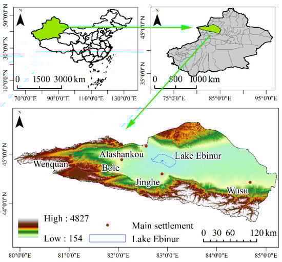
Figure 1.
Location of the study area.
2.2. Data Sources
The data used in this study can be described as follows: (1) The elevation data are based on the 90-m digital elevation model (DEM) of Shuttle Radar Topographic Mission (SRTM) data and were obtained from the Geospatial Data Cloud Platform of the Computer Network Information Center of the Chinese Academy of Sciences (http://www.gscloud.cn/ accessed on 27 November 2021). (2) The global land cover data, with a resolution of 1 km, were obtained from the University of Maryland (http://app.earth-observer.org/data/basemaps/images/global/LandCover_512/LandCoverUMD_512/LandCoverUMD_512.html/ accessed on 27 November 2021), and the Terra and Aqua combined Moderate Resolution Imaging Spectroradiometer (MODIS) Land Cover Type (MCD12Q1) Version 6 data from the USGS EROS Center (http://doi.org/10.5067/MODIS/MCD12Q1.006/ accessed on 27 November 2021), has a resolution of 500 m and uses two images (2001 and 2017). (3) The soil data were taken from the 0.5-degree soil data available for the VIC model released by the University of Washington (https://vic.readthedocs.io/en/master/Datasets/Datasets/ accessed on 27 November 2021) and based on the World Soil Database (HWSD) 1:1 million Chinese soil dataset (v1.1). (4) The meteorological data were obtained from the daily dataset of surface climate data in China (V3.0), the time resolution is daily and the time scale is from 1 January 1960 to 31 December 2017. The data were obtained from the China Meteorological Data Network (http://data.cma.cn/ accessed on 27 November 2021). (5) The verification data of LST were obtained from a combined Terra and Aqua MODIS LST and meteorological station data product for China from 2003 to 2017 [37] with a resolution of 5.6 km. The model resolution is 8 km*8 km, and the basin is divided into 767 grids (Figure 2).
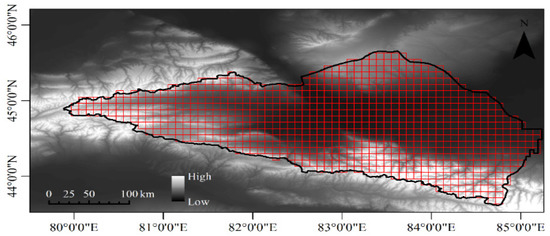
Figure 2.
Schematic diagram of the model grid.
2.3. VIC Model
The VIC hydrological model is a large-scale hydrological model with a variable infiltration capacity. The VIC model is an open-source large-scale distributed conceptual hydrological model based on one kind of water and heat balance and physical dynamic mechanisms (VIC’s homepage: http://vic.readthedocs.org/en/master/ accessed on 27 November 2021). Specific theoretical references include [38,39].
The energy balance calculation of the VIC-3L model mainly consists of four parts: LST, sensible heat flux, latent heat flux, and geothermal change. The other three parts are determined by LST, and the connecting factor of water balance and energy balance is latent heat flux. In an ideal situation, the energy balance calculation formula of each land cover type in the grid unit is as follows:
where, Rn is net radiation (W/m2), H is sensible heat flux (W/m2), is latent heat flux (W/m2), and G is surface heat flux (W/m2). The net radiation is calculated by the following formula:
where, is the surface reflectance (%) of a certain land cover type, RS is the downward short-wave radiation (), is the specific emissivity(%), RL is the downward long-wave radiation (), and is the Stefan-Boltzmann constant ( = 5.67 × 10⁻⁸ W/(m2·°C4)). The calculation formula of sensible heat is as follows:
where, Ts is the LST (°C), Ta is the atmospheric temperature (°C), and rh is the aerodynamic impedance (s/m). The surface heat flux is estimated by the heat of two layers of soil. For the upper layer (the first layer + the second layer), the total depth is assumed to be D1 (m), then its calculation formula is:
where, is the soil thermal conductivity(W/m·°C), T1 is the temperature of the upper soil (°C). Assuming that the depth of the underlying soil is D2 (m) and the temperature at the bottom of the soil is constant, then:
where, CS is the coefficient of soil heat conductivity (J/m3·°C), and is the soil temperature (°C) at the beginning and the end of the period in the upper soil respectively, and T2 is the constant temperature (°C) of the lower soil. Currently, it is believed that and CS do not change with the change of soil moisture content. According to Equations (4) and (5), the calculation formula of surface heat flux can be deduced as follows:
Combined with the above formula, the LST, sensible heat flux and surface heat flux can be calculated through iteration.
2.4. Wavelet Analysis
2.4.1. Morlet Continuous Wavelet
The long-term LST changes have obvious periodic characteristics, and there is less analysis of the multi-scale time characteristics between LST and meteorological elements. The wavelet analysis method has a powerful multi-scale resolution function, which can detect the response period of meteorological elements and LST, and can also show multiple change cycles hidden in the time series, reflecting the changing trend of the system within the same time range. Therefore, the wavelet analysis is more advantageous when studying the multi-scale characteristics of LST and meteorological elements. In this paper, we used the toolbox provided by Grinsted et al. [40], you can download it from this address: (http://www.glaciology.net/wavelet-coherence/ accessed on 27 November 2021).
The Morlet continuous wavelet function is a commonly used complex wavelet function. It has the advantages of rich phase information, good time aggregation, and high-frequency resolution. Therefore, it is widely used to study the correlation between two non-stationary sequences [41,42]. Therefore, this study selected the Morlet wavelet to analyze the degree of correlation between the LST and each meteorological element. Morlet wavelet is a complex wavelet, and its expressions in the time domain and frequency domain are:
In the formula, is a constant, and i is an imaginary number. Morlet wavelet is a single-frequency negative sine function under the Gaussian envelope. When using wavelets for feature extraction purposes the Morlet wavelet (with ) is a good choice, since it provides a good balance between time and frequency localization.
2.4.2. Cross-Wavelet Transform (XWT)
Similar to the Fourier transform, according to the description of the transformed sequence energy in Perseval’s theorem, that is, after the signal is transformed from the time domain to the frequency domain, the total energy remains unchanged, then the local time sequence x(t) The expression of Wavelet Power Spectrum (Wavelet Power Spectrum, WPS) is:
The above-mentioned continuous wavelet transform is only a one-dimensional sequence of the wavelet transform, and this research mainly involves the correlation of twotime series. In the early research, it is necessary to perform a one-dimensional wavelet transform on each sequence separately, while Hudgins et al. [43], the XWT can not only directly analyze the correlation between two time series at different frequencies, but also reflect their phase information and local characteristics in the time domain and frequency domain. For any two series of time x(t) and y(t), the expression of the XWT is:
In the formula, the wavelet transforms of the two time series x(t) and y(t) are and respectively. The corresponding wavelet cross power (Cross Wavelet Power, XWP) is [44].
2.4.3. Wavelet Coherence (WTC)
WTC is to identify the possible relationship between two time series by finding the common points of two time series in different time scales and frequency ranges. It is a kind of enhanced time-frequency correlation. Recognition tool that can express the local coherence of the XWT in the time-frequency domain [45]. Even if they correspond to the low-energy region of the XWT, their correlation in the WTC spectrum may be significant. The expression of complex wavelet coherency (Complex Wavelet Coherency) is:
In the formula, S is a smooth spectrum operation in the time domain and the frequency domain. WTC is the absolute value of complex WTC. The mathematical expression is:
3. Results
3.1. Accuracy Verification
The selection of the best model parameters is the main factor that affects the simulation accuracy of the VIC model. There are seven main parameters that need to be input to the VIC model: the storage volume curve index B; the maximum base flow velocity Dm (m3/s); the nonlinear base flow velocity Ds (m3/s); the soil moisture content Ws (%); and the three layers of soil thickness d1, d2 and d3 (m) during the nonlinear base flow. The selection of model parameters was based on traditional parameter calibration methods [46]. The above parameters were adjusted according to the empirical interval of the hydrological parameters to make the peak discharge value match the measured data. The above steps were repeated several times until a satisfactory result was obtained. The parameters are calibrated by repeatedly calculating the NSE and R2 of the simulated and the measured values of runoff. The NSE and R2 of the monthly runoff of Wenquan hydrological station during the verification period (2002–2017) are 0.44 and 0.47, respectively. The Final selected parameters are described as follows (Table 1):

Table 1.
Seven parameters of the VIC model.
3.1.1. Accuracy Verification in Terms of Time
By correctly inputting various parameters and running the model, a dataset of daily values of the LST from 1960 to 2017 can be obtained. To ensure the accuracy of the simulation, the average monthly and yearly LSTs of 6 meteorological stations (Jinghe Station, Tuoli Station, Kelamayi Station, Wusu Station, and Alashankou Station) from 1960 to 2017 were calculated as the actual measured values for this time. The results were verified, the determination coefficient R2, the Root Mean Squared Error RMSE, the Mean Absolute Error MAE, the Nash-Sutcliffe efficiency coefficient NSE were selected to evaluate the simulation accuracy of the model. The R2, RMSE, MAE, NSE values of annual simulated LSTs are 0.51 2.21, 1.85, and 0.17, respectively (Figure 3b). The R2, RMSE, MAE, NSE values of monthly simulated LSTs are 0.98, 3.93, 3.31, and 0.93, respectively (Figure 3d). It can be seen from the respective boxplots (Figure 3e,f) that the difference between the simulated and measured monthly data is not very large. The medians are 11.11 °C and 11.65 °C respectively. The measured values are slightly higher. The simulated and measured annual values have a large gap. They are 8.56 °C and 10.07 °C, the difference is 1.5 °C, our simulated values are underestimated.
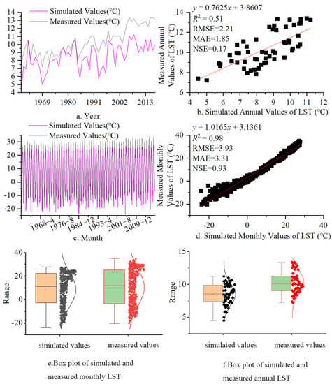
Figure 3.
(a). Comparison of LST changes between measured and simulated annual values. (b). Verification accuracy of measured and simulated annual value LST. (c). Comparison of LST changes between measured and simulated monthly values. (d). Verification accuracy of measured and simulated monthly value LST. (e,f). Boxplot of monthly and annual simulated and measured value, respectively.
3.1.2. Accuracy Verification in Terms of Space
In addition to verifying the LST over time, its spatial accuracy should be verified as well. Therefore, according to the remote sensing LST inversion dataset in China, the simulated LST based on the VIC model and its spatial distribution were compared and studied. However, through verification, it was found that the accuracy of the LST simulated by the VIC model for cold months is inaccurate, especially in January and December, where the LST is even greater than 0 in high-altitude mountainous areas in winter. According to Koch’s research [30], who found that the warmth of the VIC model in cold months is obvious, VIC has a distinct seasonality in its bias with a warm bias in winter (~3 °C) as opposed to a slight cool bias in summer (~−1 °C), which is related to an underestimation of the actual evapotranspiration and altitude. Our study area is located in an arid area, and the actual evapotranspiration in winter is small, which does not affect the accuracy of the LST simulated by the VIC model for areas other than high-altitude mountainous areas. To ensure the reasonableness of the data, the simulated LST values of the high-altitude mountainous area in November, January and December were deleted and converted to a no-data area. Taking 2017 as an example, the spatial resolutions were 0.05° and 1/12° respectively, as shown in Figure 4. It can be seen that the LST simulated by the VIC model has a high spatial consistency with the measured LST. The LST in the higher altitude area is significantly lower than that in other areas. As the time changes, the LST inside and outside the basin both “increase first and then decrease”, and the simulated LST is slightly lower than the measured data.
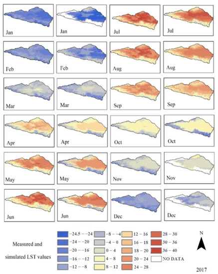
Figure 4.
Spatial comparison map of simulated and measured LSTs in the Ebinur Lake Watershed.
Of course, the accuracy needs to be improved, but for the data-scarce area, the simulation results can provide continuous and long-term serial data support, which has certain advantages.
3.2. Temporal and Spatial Variation Characteristics of the LST
The overall trend of the daily average LST in the study area was a unimodal distribution. The daily average LST (Figure 5, left) began to increase at the end of February, reached the maximum in mid-July, began to decline at the end of August, and reached the minimum at the end of January. The peak in mid-July (July 13) was 25.92 °C, and the LST dropped rapidly to the lowest value in late January (January 22) at −18.99 °C. The daily average LST of the entire study area was 6.95 °C.
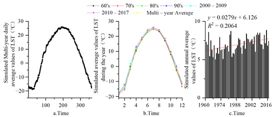
Figure 5.
Temporal changes of daily (a), monthly (b) and annual average (c) LST in the Study area.
The monthly average LST in the study area also showed a single-peak trend (Figure 5, middle). The peak monthly average LST appeared in July. The order of the July peaks in each decadal period was 2010–2017 > 80s > 90s > 2000–2009 > 70s > 60s, and the peak values were 26.06 °C, 25.60 °C, 25.58 °C, 25.41 °C, 25.07 °C and 24.89 °C, respectively.
A histogram was used to represent the distribution of the annual average LST from 1960 to 2017 (Figure 5, right). The figure shows that the average annual LST is on the rise, with a rising rate of approximately 0.0279 °C/a and an increase of approximately 1.62 °C in the past 58 years. The annual average LST is 6.40 °C. The annual average LST reached a trough in 1960, with a value of 4.54 °C; the figure clearly shows that the annual average LST after 2000 was significantly higher than that before 2000, which may be caused by increasing human activities, the industrial and agricultural activities in the Ebinur Lake Watershed.
Based on the values of the daily LST simulated by the VIC model, the spatial distribution map of the inter-decadal and multi-year average LSTs from 1960 to 2017 was calculated. It can be seen that there are no obvious differences in the LST in the basin, but there are varying degrees of variation between different decadal periods.
The LST changes within the basin are not obvious, and the degree of change is different (Figure 6). The main manifestation is the gradual decrease of the high LST areas in the east and the gradual increase of the central LST. The LST range changed from −11.48–9.04 °C in the 1960s to −11.14–9.56 °C in the 1980s, and then to −3.5–10.51 °C in 2010–2017, with the average values being 3.28 °C, 5.24 °C, and 6.79 °C, respectively. These results show that the LST in this area has an increasing trend. Although the range of high-value areas in the east has decreased, gradually shrinking to the low vegetation coverage area near Lake Ebinur, the LST value has increased, and the multi-year average LST in other regions has increased compared with the values in the 1960s. Therefore, the LST of the basin is increasing.
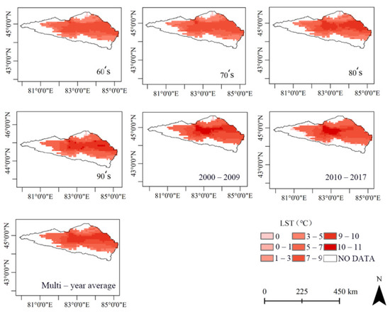
Figure 6.
Interdecadal changes and annual mean LST spatial distribution in the Ebinur Lake Watershed.
3.3. Delayed Correlation Analysis of LST and Meteorological Elements
The XWT and WTC of the dual time series were applied to the coefficients after continuous wavelet transform, and the XWT spectrum between the LST of the Ebinur Lake Watershed and other meteorological elements was obtained (Figure 7) and crossed with the WTC spectrum (Figure 8). The XWT and WTC can well reflect the “correlation” between changes in two different time series. The XWT generally reflects the strength of the “shared period” between sequences. The WTC generally reflects the consistency of the periodic “change trend” between sequences but does not directly reflect the intensity relationship of the change period. As shown in Figure 7 and Figure 8, the meteorological elements and LST of the basin are bounded by 1989. The two figures together show the following:
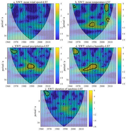
Figure 7.
XWT analysis of mean wind speed and LST (a), XWT analysis of mean temperature and LST (b), XWT analysis of annual precipitation and LST (c), XWT analysis of relative humidity and LST (d), XWT analysis of duration of sunshine and LST (e). (Note: The horizontal axis of the wavelet period diagram corresponds to the time of the original time series, the vertical axis represents the period of change, and the color represents the intensity of the change period. In this figure, yellow represents the high intensity of the change cycle. The thin solid line is the Cone of Influence (COI), and only the energy spectrum within this solid line needs to be considered. In order to eliminate the interference of the boundary effect, the thick solid line represents the key value that passes the significance test with 95% confidence; the arrow indicates the relative phase difference: → indicates that the two changes in phase are consistent, ← indicates that the two changes in phase are opposite, ↑ indicates that the phase change of the meteorological element is 90° ahead of the LST phase, and ↓ indicates that the phase change of the meteorological element is 90° behind the LST phase [47,48]). (The same below).
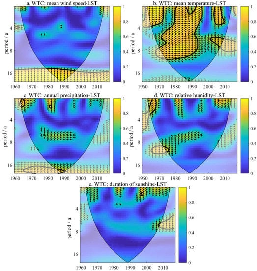
Figure 8.
WTC analysis of mean wind speed and LST (a), WTC analysis of mean temperature and LST (b), WTC analysis of annual precipitation and LST (c), WTC analysis of relative humidity and LST (d), WTC analysis of duration of sunshine and LST (e). (Note: The right axis generally reflects the consistency of periodic "change trends" between sequences, similar to the correlation coefficient. The larger the coefficient, the higher the correlation and the more consistent the change.).
In the power spectrum of XWT, there was a significant area with a period of 1~2a in the average wind speed and LST from 1962 to 1966, the correlation is approximately positive; there are 4 significant areas between the average temperature and the LST, which are approximately 1.5a (1964–1967), 1~3a (2003–2008), 5.5–7a (2005–2009) and 7~9a (1984–1990). The two showed a positive correlation between the average temperature and the LST; the annual precipitation and the LST had significant areas of 0.5~2a and 6~8a in 1964–1972 and 1984–1994, respectively. Both have an approximately negative correlation; relative humidity and annual precipitation are the same, and there are significant areas of 1~2a and 6~9a in 1964–1971 and 1978–1994, respectively, and the two also show a similar negative correlation. Sunshine hours and LST only existed in a significant area of 1~2a from 1964 to 1970, and the two are in an approximately positive correlation.
In the coherence spectrum of WTC, the average wind speed and surface temperature have a significant area greater than 15 years from 1980 to 1996, and the average wind speed in this area is ahead of the surface temperature, that is, 1/4a ahead of time; the average temperature and the surface temperature in the area with the 95% confidence interval accounted for more than 60%, indicating that the average temperature is the main controlling factor of the surface temperature, and the two existed in 1963–1972, 1980–1996 and 2004–2010 on the time scale of 1~4a. For significant periods, most areas of the two are approximately positively correlated. Among them, there may be abrupt changes around 1980 and 1996 on the time scale of 1~2a; that is, there may be a “high-low” transition of surface temperature, and there are still two significant cycles of ~10a (1970–1994) and 5~7.5a (2000–2009); the annual precipitation and surface temperature only have a small cycle of 1~1.5a (1964–1966), and the two are negatively correlated; the other periodic feature is not obvious; the relative humidity and surface temperature have a significant area of 1~2.5a from 1964 to 1968 and a negative correlation, and the other two periodic features are not obvious; the sunshine hours and surface temperature have only one area where the periodic characteristics are not obvious.
3.4. The Impact of LUCC on LST
The statistics were classified according to the three-phase LUCC in this study. The specific changes in land cover types in the 1990s, 2001, and 2017 are shown in Figure 9 and Figure 10, and the range distribution of the LST in the corresponding time period is shown in Figure 11.
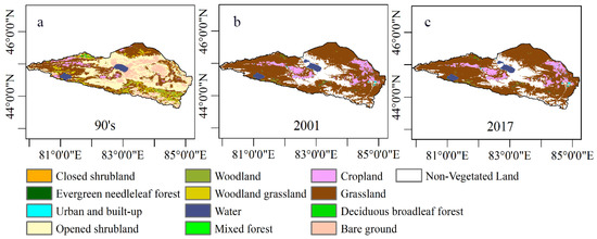
Figure 9.
Distribution of LUCC in the study area in the 90’s (a), in 2001 (b), in 2017 (c).
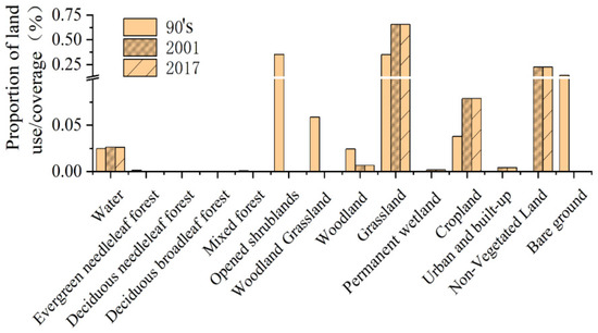
Figure 10.
Changes in LUCC in the Ebinur Lake Watershed.
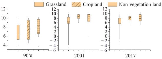
Figure 11.
Box plots of LST.
The order of land cover types in the Ebinur Lake Watershed in the 1990s (Figure 9a) was open shrubland > grassland > bare ground > woodland grassland > crop land > water > woodland > evergreen needleleaf forest > mixed forest > urban and built-up > deciduous broadleaf forest. Among them (Figure 10), the largest area of open shrubland was 18,587.6 km2, accounting for 35.1% of the total area, followed by grassland, with an area of 18,476.3 km2, accounting for 34.9% of the total area. Bare ground accounted for 13.9% of the total area, and cropland accounted for 3.8% of the total area. Deciduous broadleaf forest occupied the smallest area, accounting for only 0.14% of the total area.
The order of land cover types in the Ebinur Lake Watershed in 2001 (Figure 9b) was grassland > non-vegetation land > cropland > water > woodland > urban and built-up > permanent wetland > evergreen needleleaf forest > deciduous broadleaf forest > mixed forest > woodland grassland > open shrubland > deciduous needleleaf forest. Among them (Figure 10), the area of grassland has increased, reaching the largest area of 34,714.9 km2 and accounting for 65.6% of the total area, followed by non-vegetation land with an area of 11,904.9 km2, accounting for 22.5% of the total area. The two accounted for 88.1% of the total area. The area of cropland decreased to 4184.4 km2, accounting for only 7.9% of the total area. The area of open shrubland dropped sharply, most of them were transformed into grassland or non-vegetation land.
The order of land cover types in the Ebinur Lake Watershed in 2017 (Figure 9c) was grassland > non-vegetation land > cropland > water > woodland > urban and built-up > permanent wetland > evergreen needleleaf forest > deciduous broadleaf forest > mixed forest > woodland grassland > open shrubland > deciduous needleleaf forest. This is consistent with the ranking in 2001, and the area has not changed much. Grassland and non-vegetation land are also the main land cover types in the study area (Figure 10).
In the 90s, the LST of grassland ranged from 5.2 to 8.4 °C, with a median of 6.3 °C; the LST of cropland ranged from 5.3 to 9.5 °C, with a median of 8.1 °C; the LST of non-vegetation land was in the range of 6.5–9.7 °C, with a median of 8.4 °C.
In 2001, the LST of grassland ranged from 5.7 to 8.5 °C, with a median of 6.6 °C; the LST of cropland ranged from 7.9 to 9.7 °C, with a median of 8.7 °C; the LST of non-vegetation land was in the range of 6.6–9.7 °C, with a median of 8.1 °C.
In 2017, the LST of grassland ranged from 5.5 to 8.0 °C, with a median of 6.2 °C; the LST of cropland ranged from 7.1 to 8.7 °C, with a median of 8.3 °C; the LST of non-vegetation land was in the range of 6.7–9.6 °C, with a median of 7.8 °C.
During the period, the area of open shrubland, most of which was converted to grassland, cropland, and non-vegetation land, declined sharply; the area of grassland increased most obviously, and the LST was lower. Although the area of cropland was small, the LST was higher; compared with land types with higher vegetation coverage such as grassland, the LST of non-vegetation land was higher, which may have been because a large amount of solar radiation was absorbed by vegetation, lowering its LST.
4. Discussion
4.1. Harmful Effects Caused by Changes in LST in Arid Regions
On the global scale, arid regions cover approximately one-third of the earth [49], and are one of the most sensitive regions to wind erosion phenomena [50]. In some recent research, a positive association was observed between the LST and wind erosion events [16,18]. The soil system has a synergistic relationship between various physical and chemical processes and environmental variables that affect its development [51]. Increasing the LST and decreasing the soil moisture, especially in the warm seasons over the arid regions, can be a factor in exacerbating soil erosion due to their effect on the salt accumulation on the soil surface [16,52]. Meanwhile, Different LUCC trends have different effects on the LST [53]. Heat sources (including bare land, urban and built-up land, and cropland) increase the LST, while cold sources (woodland, grassland, and water) reduce the LST [54]. Cropland and bare ground have a great impact on the regional LST, which is mainly reflected in the area and intensity of the impact [55]. This study found that between 1960 and 2017, the amount of open shrubs in the Ebinur Lake Watershed decreased sharply, and most of these areas were converted to grassland, cropland, and non-vegetation land. The vegetation coverage in the above-mentioned areas was low, and the LST was relatively high. This finding reasonably explains the variation in the LST of the Ebinur Lake Watershed from 1960 to 2017. However, the increased LST will lead to the reduction of regional soil moisture, vegetation degradation, and even increase the frequency of wind erosion and dust emission events. We believe this should attract the attention of local society.
4.2. Evaluation of VIC Model for LST Simulation
The LST is an important and complex hydrological state variable of land-atmosphere interactions. Land surface models (LSMs), such as the VIC model, are a key tool for enhancing the understanding of the process and providing predictions of the coupling between the terrestrial hydrosphere and its atmosphere. Distributed LSMs can be used to understand the hydrological status and flux of each grid cell, such as the LST. By comparing and analyzing the simulation accuracy of three different LSMs, Koch et al. [30] found that they all have certain spatial defects. The VIC has a distinct seasonality in its bias with a warm bias in winter (~3 °C) as opposed to a slight cool bias in summer (~−1 °C). The VIC model has a better simulation effect on the LST in warm months; in cold months, underestimation of the actual evapotranspiration will result in a high LST simulation. In this study, the same situation also appeared, but it may be because the study area is located in an arid area, that is, the actual evapotranspiration in autumn and winter, which are cold months, is inherently low, so except for high-altitude mountainous areas, the accuracy of the LST in cold months in plain areas is still good. However, the LST in high-altitude mountainous areas is obviously overestimated, only in November, December and January there is a big deviation in the mountainous area, and the LST in the areas close to the Tianshan Mountains is greater than zero in winter, which is unlikely to happen. This lack of spatial accuracy may be related to the occurrence of snow in mountainous areas, but further analysis is needed to study this in more detail.
5. Conclusions
This study used the VIC model to simulate the LST of the Ebinur Lake Watershed from 1960 to 2017, analyzed its temporal and spatial characteristics, conducted a multiscale cross-analysis of various meteorological elements and LST, analyzed the correlations between LUCC and LST, and obtained the following conclusions:
- Although the model simulates the LST well in time and the space verification results are relatively good, the LST simulation in the high-altitude area of the cold month is seriously overestimated, which may be related to the occurrence of snowfall or to the altitude. Further research is needed.
- The LST of the Ebinur Lake Watershed shows an overall increasing trend, and the annual average LST is higher in the central and eastern parts of the basin. On the temporal scale, the daily and monthly average LSTs showed unimodal trends. The interdecadal monthly changes are not obvious, and the monthly average LST from 2010 to 2017 fluctuates more than in other periods.
- It is worth mentioning that there is a sudden change affected by the mean LST on a time scale of 1~2a (1980–1996); that is, there is a “strong-weak” transition in the LST.
- From 1960 to 2017, the LUCC of the Ebinur Lake Watershed underwent major changes, and the reduction of open shrubs may have caused the LST increase in this area.
Author Contributions
N.A. conceived and designed the experiments, performed the experiments, analyzed the data, contributed reagents/materials/analysis tools, prepared figures and/or tables, authored or reviewed drafts of the paper, approved the final draft. J.D. conceived and designed the experiments, contributed reagents/materials/analysis tools, authored or reviewed drafts of the paper, approved the final draft. All authors have read and agreed to the published version of the manuscript.
Funding
This research was funded by National Natural Science Foundation of China (no. 42171269); Xinjiang Academician Workstation Cooperative Research Project (no. 2020.B-001); National Natural Science Foundation of China (no. 41771470); National Natural Science Foundation of China (no. 4196105).
Acknowledgments
Sincere thanks are extended to the teachers and students of the Key Laboratory of Oasis Ecology Department of Xinjiang University for their support and help. Furthermore, the authors would like to thank the reviewers and editors for providing helpful suggestions to improve this manuscript.
Conflicts of Interest
The authors declare no conflict of interest.
References
- Stocker, T. Climate Change 2013: The Physical Science Basis: Working Group I Contribution to the Fifth Assessment Report of the Intergovernmental Panel on Climate Change; Cambridge University Press: Cambridge, UK, 2014. [Google Scholar]
- Zhang, D.; Tang, R.; Zhao, W.; Tang, B.; Wu, H.; Shao, K.; Li, Z.-L. Surface Soil Water Content Estimation from Thermal Remote Sensing based on the Temporal Variation of Land Surface Temperature. Remote Sens. 2014, 6, 3170–3187. [Google Scholar] [CrossRef] [Green Version]
- Harris, P.P.; Folwell, S.S.; Gallego-Elvira, B.; Rodríguez, J.; Milton, S.; Taylor, C.M. An Evaluation of Modeled Evaporation Regimes in Europe Using Observed Dry Spell Land Surface Temperature. J. Hydrometeorol. 2017, 18, 1453–1470. [Google Scholar] [CrossRef] [Green Version]
- Vancutsem, C.; Ceccato, P.; Dinku, T.; Connor, S.J. Evaluation of MODIS land surface temperature data to estimate air temperature in different ecosystems over Africa. Remote Sens. Environ. 2010, 114, 449–465. [Google Scholar] [CrossRef]
- Mustafa, E.K.; El-Hamid, H.T.A.; Tarawally, M. Spatial and temporal monitoring of drought based on land surface temperature, Freetown City, Sierra Leone, West Africa. Arab. J. Geosci. 2021, 14, 4. [Google Scholar] [CrossRef]
- Panda, S.K.; Choudhury, S.; Saraf, A.K.; Das, J.D. MODIS land surface temperature data detects thermal anomaly preceding 8 October 2005 Kashmir earthquake. Int. J. Remote Sens. 2007, 28, 4587–4596. [Google Scholar] [CrossRef]
- Zhao, N.; Han, S.; Xu, D.; Wang, J.; Yu, H. Cooling and Wetting Effects of Agricultural Development on Near-Surface Atmosphere over Northeast China. Adv. Meteorol. 2016, 2016, 6439276. [Google Scholar] [CrossRef]
- Luo, D.; Jin, H.; Wu, Q.; Bense, V.; He, R.; Ma, Q.; Gao, S.; Jin, X.; Lü, L. Thermal regime of warm-dry permafrost in relation to ground surface temperature in the Source Areas of the Yangtze and Yellow rivers on the Qinghai-Tibet Plateau, SW China. Sci. Total Environ. 2018, 618, 1033–1045. [Google Scholar] [CrossRef]
- He, C.Y.; Gao, B.; Huang, Q.X.; Ma, Q.; Dou, Y.Y. Environmental degradation in the urban areas of China: Evidence from multi-source remote sensing data. Remote Sens. Environ. 2017, 193, 65–75. [Google Scholar] [CrossRef]
- Zhang, T.; Hoerling, M.P.; Perlwitz, J.; Sun, D.-Z.; Murray, D. Physics of U.S. Surface Temperature Response to ENSO. J. Clim. 2011, 24, 4874–4887. [Google Scholar] [CrossRef]
- Winterdahl, M.; Erlandsson, M.; Futter, M.N.; Weyhenmeyer, G.A.; Bishop, K. Intra-annual variability of organic carbon concentrations in running waters: Drivers along a climatic gradient. Glob. Biogeochem. Cycles 2014, 28, 451–464. [Google Scholar] [CrossRef] [Green Version]
- Li, R.; Wang, C.; Wu, D. Changes in precipitation recycling over arid regions in the Northern Hemisphere. Theor. Appl. Clim. 2018, 131, 489–502. [Google Scholar] [CrossRef] [Green Version]
- Faramarzi, M.; Heidarizadi, Z.; Mohamadi, A.; Heydari, M. Detection of vegetation changes in relation to normalized dif-ference vegetation index (NDVI) in semi-arid rangeland in western Iran. J. Agric. Sci. Technol. 2018, 20, 51–60. Available online: http://hdl.handle.net/123456789/3627 (accessed on 29 November 2021).
- Yang, L.; Sun, G.; Zhi, L.; Zhao, J. Negative soil moisture-precipitation feedback in dry and wet regions. Sci. Rep. 2018, 8, 1–9. [Google Scholar] [CrossRef]
- Kok, J.F.; Ward, D.S.; Mahowald, N.M.; Evan, A.T. Global and regional importance of the direct dust-climate feedback. Nat. Commun. 2018, 9, 1–11. [Google Scholar] [CrossRef] [PubMed]
- Ebrahimi-Khusfi, Z.; Sardoo, M.S. Recent changes in physical properties of the land surface and their effects on dust events in different climatic regions of Iran. Arab. J. Geosci. 2021, 14, 1–18. [Google Scholar] [CrossRef]
- Khusfi, Z.E.; Roustaei, F.; Khusfi, M.E.; Naghavi, S. Investigation of the relationship between dust storm index, climatic parameters, and normalized difference vegetation index using the ridge regression method in arid regions of Central Iran. Arid. Land Res. Manag. 2020, 34, 239–263. [Google Scholar] [CrossRef]
- Ryu, J.-H.; Hong, S.; Lyu Sang, J.; Chung, C.-Y.; Shi, I.; Cho, J. Effect of Hydro-meteorological and Surface Conditions on Variations in the Frequency of Asian Dust Events. Korean J. Remote Sens. 2018, 34, 25–43. [Google Scholar] [CrossRef]
- Ji, F.; Wu, Z.; Huang, J.; Chassignet, E.P. Evolution of land surface air temperature trend. Nat. Clim. Chang. 2014, 4, 462–466. [Google Scholar] [CrossRef]
- Huang, J.; Guan, X.; Ji, F. Enhanced cold-season warming in semi-arid regions. Atmos. Chem. Phys. Discuss. 2012, 12, 4627–4653. [Google Scholar] [CrossRef] [Green Version]
- Liu, Y.; Peng, J.; Wang, Y. Efficiency of landscape metrics characterizing urban land surface temperature. Landsc. Urban Plan. 2018, 180, 36–53. [Google Scholar] [CrossRef]
- Mahmood, R.; Pielke Sr, R.A.; Hubbard, K.G.; Niyogi, D.; Dirmeyer, P.A.; McAlpine, C.; Carleton, A.M.; Hale, R.; Gameda, S.; Beltrán-Przekurat, A. Land cover changes and their biogeophysical effects on climate. Int. J. Climatol. 2014, 34, 929–953. [Google Scholar] [CrossRef] [Green Version]
- Pitman, A.; Arneth, A.; Ganzeveld, L. Regionalizing global climate models. Int. J. Climatol. 2012, 32, 321–337. [Google Scholar] [CrossRef]
- Chen, L.; Dirmeyer, P. The relative importance among anthropogenic forcings of land use/land cover change in affecting temperature extremes. Clim. Dyn. 2019, 52, 2269–2285. [Google Scholar] [CrossRef]
- Ahmed, B.; Kamruzzaman, M.; Zhu, X.; Rahman, M.S.; Choi, K. Simulating Land Cover Changes and Their Impacts on Land Surface Temperature in Dhaka, Bangladesh. Remote Sens. 2013, 5, 5969–5998. [Google Scholar] [CrossRef] [Green Version]
- Turner II, B. Land system architecture for urban sustainability: New directions for land system science illustrated by application to the urban heat island problem. J. Land Use Sci. 2016, 11, 689–697. [Google Scholar] [CrossRef]
- Pal, S.; Ziaul, S. Detection of land use and land cover change and land surface temperature in English Bazar urban centre. Egypt J. Remote Sens. Space Sci. 2017, 20, 125–145. [Google Scholar] [CrossRef] [Green Version]
- Patz, J.A.; Campbell-Lendrum, D.; Holloway, T.; Foley, J.A. Impact of regional climate change on human health. Nature 2005, 438, 310–317. [Google Scholar] [CrossRef]
- Change, I.C. Mitigation of Climate Change. Contribution of Working Group III to the Fifth Assessment Report of the Intergovernmental Panel on Climate Change; IPCC: Geneva, Switzerland, 2014; p. 1454. [Google Scholar]
- Koch, J.; Siemann, A.; Stisen, S.; Sheffield, J. Spatial validation of large-scale land surface models against monthly land surface temperature patterns using innovative performance metrics. J. Geophys. Res. Atmos. 2016, 121, 5430–5452. [Google Scholar] [CrossRef]
- Yuan, F.; Xie, Z.; Liu, Q.; Yang, H.; Su, F.; Liang, X.; Ren, L. An application of the VIC-3L land surface model and remote sensing data in simulating streamflow for the Hanjiang River basin. Can. J. Remote Sens. 2004, 30, 680–690. [Google Scholar] [CrossRef]
- Wang, J.; Ding, J.; Yu, D.; Ma, X.; Zhang, Z.; Ge, X.; Teng, D.; Li, X.; Liang, J.; Lizaga, I.; et al. Capability of Sentinel-2 MSI data for monitoring and mapping of soil salinity in dry and wet seasons in the Ebinur Lake region, Xinjiang, China. Geoderma 2019, 353, 172–187. [Google Scholar] [CrossRef]
- Wang, J.; Ding, J.; Yu, D.; Teng, D.; He, B.; Chen, X.; Ge, X.; Zhang, Z.; Wang, Y.; Yang, X.; et al. Machine learning-based detection of soil salinity in an arid desert region, Northwest China: A comparison between Landsat-8 OLI and Sentinel-2 MSI. Sci. Total Environ. 2020, 707, 136092. [Google Scholar] [CrossRef]
- Wang, J.; Ding, J.; Li, G.; Liang, J.; Yu, D.; Aishan, T.; Zhang, F.; Yang, J.; Abulimiti, A.; Liu, J. Dynamic detection of water surface area of Ebinur Lake using multi-source satellite data (Landsat and Sentinel-1A) and its responses to changing environment. Catena 2019, 177, 189–201. [Google Scholar] [CrossRef]
- Zhang, J.; Ding, J.; Wu, P.; Tan, J.; Huang, S.; Teng, D.; Cao, X.; Wang, J.; Chen, W. Assessing arid Inland Lake Watershed Area and Vegetation Response to Multiple Temporal Scales of Drought Across the Ebinur Lake Watershed. Sci. Rep. 2020, 10, 1354. [Google Scholar] [CrossRef] [PubMed]
- Zhang, F.; Kung, H.; Johnson, V.C.; LaGrone, B.I.; Wang, J. Change Detection of Land Surface Temperature (LST) and some Related Parameters Using Landsat Image: A Case Study of the Ebinur Lake Watershed, Xinjiang, China. Wetlands 2018, 38, 65–80. [Google Scholar] [CrossRef]
- Zhao, B.; Mao, K.; Cai, Y.; Shi, J.; Li, Z.; Qin, Z.; Meng, X.; Shen, X.; Guo, Z. A combined Terra and Aqua MODIS land surface temperature and meteorological station data product for China from 2003 to 2017. Earth Syst. Sci. Data 2020, 12, 2555–2577. [Google Scholar] [CrossRef]
- Tang, C.; Piechota, T.C. Spatial and temporal soil moisture and drought variability in the Upper Colorado River Basin. J. Hydrol. 2009, 379, 122–135. [Google Scholar] [CrossRef]
- Umair, M.; Kim, D.; Ray, R.L.; Choi, M. Estimating land surface variables and sensitivity analysis for CLM and VIC simulations using remote sensing products. Sci. Total Environ. 2018, 633, 470–483. [Google Scholar] [CrossRef] [PubMed]
- Grinsted, A.; Moore, J.; Jevrejeva, S. Application of the cross wavelet transform and wavelet coherence to geophysical time series. Nonlinear Process. Geophys. 2004, 11, 561–566. [Google Scholar] [CrossRef]
- Torrence, C.; Compo, G. A Practical Guide to Wavelet Analysis. Bull. Am. Meteorol. Soc. 1997, 79, 61–68. [Google Scholar] [CrossRef] [Green Version]
- Aguiar-Conraria, L.; Soares, M. The Continuous Wavelet Transform: A Primer; NIPE Working Papers; Universidade do Minho: Braga, Portugal, 2010. [Google Scholar]
- Hudgins, L.; Friehe, C.A.; Mayer, M.E. Wavelet transforms and atmopsheric turbulence. Phys. Rev. Lett. 1993, 71, 3279–3282. [Google Scholar] [CrossRef]
- Lau, K.M.; Weng, H. Climate Signal Detection Using Wavelet Transform: How to Make a Time Series Sing. Bull. Am. Meteorol. Soc. 1995, 76, 2391–2402. [Google Scholar] [CrossRef] [Green Version]
- Huang, H.B.; Huang, X.R.; Yang, M.L.; Lim, T.C.; Ding, W.P. Identification of vehicle interior noise sources based on wavelet transform and partial coherence analysis. Mech. Syst. Signal Process. 2018, 109, 247–267. [Google Scholar] [CrossRef]
- Troy, T.J.; Wood, E.; Sheffield, J. An efficient calibration method for continental-scale land surface modeling. Water Resour. Res. 2008, 44, W09411. [Google Scholar] [CrossRef]
- Onderka, M.; Banzhaf, S.; Scheytt, T.; Krein, A. Seepage velocities derived from thermal records using wavelet analysis. J. Hydrol. 2013, 479, 64–74. [Google Scholar] [CrossRef]
- Su, L.; Miao, C.; Borthwick, A.G.; Duan, Q. Wavelet-based variability of Yellow River discharge at 500-, 100-, and 50-year timescales. Gondwana Res. 2017, 49, 94–105. [Google Scholar] [CrossRef] [Green Version]
- Wang, J.; Shi, T.; Yu, D.; Teng, D.; Ge, X.; Zhang, Z.; Yang, X.; Wang, H.; Wu, G. Ensemble machine-learning-based framework for estimating total nitrogen concentration in water using drone-borne hyperspectral imagery of emergent plants: A case study in an arid oasis, NW China. Environ. Pollut. 2020, 266, 115412. [Google Scholar] [CrossRef] [PubMed]
- Reynolds, R.L.; Yount, J.C.; Reheis, M.; Goldstein, H.; Chavez, P., Jr.; Fulton, R.; Whitney, J.; Fuller, C.; Forester, R.M. Dust emission from wet and dry playas in the Mojave Desert, USA. Earth Surf. Process. Landf. 2007, 32, 1811–1827. [Google Scholar] [CrossRef]
- Wang, J.; Hu, X.; Shi, T.; He, L.; Hu, W.; Wu, G. Assessing toxic metal chromium in the soil in coal mining areas via proximal sensing: Prerequisites for land rehabilitation and sustainable development. Geoderma 2022, 405, 115399. [Google Scholar] [CrossRef]
- Balba, A.M. Management of Problem Soils in Arid Ecosystems; CRC Press: Boca Raton, FL, USA, 2018. [Google Scholar]
- Fu, P.; Xie, Y.; Weng, Q.; Myint, S.; Meacham-Hensold, K.; Bernacchi, C. A physical model-based method for retrieving urban land surface temperatures under cloudy conditions. Remote Sens. Environ. 2019, 230, 111191. [Google Scholar] [CrossRef]
- Shao, Z.; Zhang, L. Estimating Forest Aboveground Biomass by Combining Optical and SAR Data: A Case Study in Genhe, Inner Mongolia, China. Sensors 2016, 16, 834. [Google Scholar] [CrossRef] [Green Version]
- Liu, T.; Zhang, S.; Yu, L.; Bu, K.; Yang, J.; Chang, L. Simulation of regional temperature change effect of land cover change in agroforestry ecotone of Nenjiang River Basin in China. Theor. Appl. Clim. 2017, 128, 971–981. [Google Scholar] [CrossRef]
Publisher’s Note: MDPI stays neutral with regard to jurisdictional claims in published maps and institutional affiliations. |
© 2021 by the authors. Licensee MDPI, Basel, Switzerland. This article is an open access article distributed under the terms and conditions of the Creative Commons Attribution (CC BY) license (https://creativecommons.org/licenses/by/4.0/).