Abstract
In the northeastern United States, widespread deforestation occurred during the 17–19th centuries as a result of Euro-American agricultural activity. In the late 19th and early 20th centuries, much of this agricultural landscape was reforested as the region experienced industrialization and farmland became abandoned. Many previous studies have addressed these landscape changes, but the primary method for estimating the amount and distribution of cleared and forested land during this time period has been using archival records. This study estimates areas of cleared and forested land using historical land use features extracted from airborne LiDAR data and compares these estimates to those from 19th century archival maps and agricultural census records for several towns in Massachusetts, a state in the northeastern United States. Results expand on previous studies in adjacent areas, and demonstrate that features representative of historical deforestation identified in LiDAR data can be reliably used as a proxy to estimate the spatial extents and area of cleared and forested land in Massachusetts and elsewhere in the northeastern United States. Results also demonstrate limitations to this methodology which can be mitigated through an understanding of the surficial geology of the region as well as sources of error in archival materials.
1. Introduction
English colonization of southern New England, a region in the northeastern United States, began in the early 17th century and initiated a drastic change from previous land use activities practiced by Native American groups who had inhabited the region for thousands of years [1,2,3,4]. English-style agriculture was much different than what had previously been practiced in the region, and required widespread deforestation to create a landscape of bounded fields for tillage, pasture, and mowing, punctuated by managed woodlots [3,5,6]. This region had been glaciated up until ~16,000–17,000 years ago [7], and agricultural fields were typically developed on glacial till, which was full of large stones and boulders. As forests were cleared, loose stones and boulders on the surface were organized into stone walls [6]. It was also more difficult for soils to retain moisture, and soil temperature fluctuated drastically, causing deeper freezing of the ground surface [3,6]. These temperature fluctuations combined with plowing for agriculture brought stones deeper in the soil column to the surface, where they required removal for successful agricultural pursuits by farmers [3,5,6]. Over decades, stones uncovered during plowing were moved to the edges of fields for disposal and continually added to the stone walls, demarcating property boundaries and individual fields within, and providing fencing. The material also provided a more durable, available, and affordable alternative to timber [6,8,9,10] and was widely used throughout the region, which is now well-known for its stone walls [6,11]. During the initial stages of English settlement, or in areas with a lower percentage of glacial till, other materials were likely used for fencing, or used in combination with stone for fencing, including brush and tree stumps; these were eventually replaced with rail or stone and rail fencing as stone became available [8,9]. Overall, the combination of deforestation and plowing was responsible for a vast number of impacts in this region, ranging from changes in ecology [12] and climate [13], to widespread topsoil erosion which irrevocably altered the fluvial systems in the region [3,14].
Additional deforestation and soil impacts in the region were caused by the production of charcoal for the iron industry, which reached its peak in the area during the mid-19th century [9,15]. Large swaths of forest were cleared, and trees were processed into charcoal upon round earthen platforms, which were known by a variety of contemporary names [9], and referred to here as relict charcoal hearths (RCHs). These were built and monitored by colliers who lived in nearby dwellings. Nearby areas in western New England, eastern New York, and Pennsylvania were highly active in iron production during this time period, with charcoal needed daily to fuel iron furnaces [15,16,17]. Charcoaling was common in southern New England, and studies have shown it was also common throughout the eastern U.S. as well as in certain parts of Europe [18,19,20,21,22,23,24]. Charcoaling was widespread in forested non-agricultural areas, which were usually rugged terrain that was not suitable for agriculture [9,20], though not all rugged and forested terrain in the region was used for charcoaling and was also often used for woodlots associated with farms. Charcoaling also occurred on more localized scales where individual farmers may have produced it; in these cases, it is possible that charcoaling could have occurred in fallow fields or other areas associated with the farm [9,25].
The height of deforestation in this region generally occurred in the mid-19th century (1850–1880), but varied by state and also by town—some towns experienced later peaks than others if they were further inland [26]. Inland areas further north and west, such as Maine, Vermont, and New York, were part of later settlement as younger generations moved in search of land, and these processes occurred there much later than areas in southeastern New England (Figure 1). Generally, by the late 19th and early 20th centuries, many fields, pastures, and other deforested areas which had been improved farmland became reforested as farm families in the region moved to cities to look for different types of work and farmland became abandoned [25,27,28].
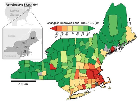
Figure 1.
Change in improved land (km2) in the northeastern U.S. by county, 1850–1870, compiled from U.S. Census Nonpopulation Schedule for Agriculture data [29,30]. This census recorded the amount of improved and unimproved farmland at the town level beginning in 1850. Counties in gray did not exist in 1850 and therefore continuous data are not available. Map projection is NAD 1983 UTM Zone 18N. Abbreviations for states in the inset map are as follows: CT, Connecticut; MA, Massachusetts; ME, Maine; NH, New Hampshire; NY, New York; RI, Rhode Island; VT, Vermont.
The northeastern U.S. is now considered to be one of the most densely forested areas currently in the United States [31], and it is estimated that 65–90% is reforested [32], with only ~450 ha of old growth forest throughout Massachusetts, primarily located in the northwestern part of the state. Many of the tracts are <10 ha and located in steep, rugged terrain [33]. Research is ongoing to determine the impacts of historical widespread deforestation and subsequent reforestation since many aspects are still poorly understood. Examples include impacts to forest ecology [34,35], geomorphology [14,36,37,38], regional climate [13], and wildlife biology [39]. For example, Hall et al. found that at local scales, historical land use imparted strong impacts on local vegetation, but since land use was homogenous throughout Massachusetts, averaging over broad spatial scales reduced variation [34].
Airborne Light Detection and Ranging (LiDAR) has been most commonly used to generate digital elevation models (DEMs) of the land surface and has therefore allowed for the widespread study of historical human impacts on the landscape, as it is effective at discerning extant cultural features in forested areas. Over the past ~15 years, as datasets become more widespread and of higher resolution, LiDAR has revealed the extent of human impacts on the land surface in many regions of the world, including New England [40,41,42,43,44,45,46,47]. Extant historical land use features that are indicative of past deforestation, specifically stone walls and relict charcoal hearths (RCHs), are widespread throughout the landscape in the northeastern U.S., and since they have topographic signatures, they are visible using airborne LiDAR [9] (Figure 2). Using various visualization techniques, features of interest are identified, extracted, and analyzed, and more recent studies have explored automated methods for feature extraction [20,41,48,49,50,51,52]. Study areas vary on a global scale, as do the time periods which are being studied, especially since features from different time periods exist contemporaneously on the landscape as a palimpsest when viewed in a LiDAR DEM [53,54,55]. Availability of complementary sources that can be used in analyses of these features, such as archival data, also vary, and this can influence the types of analyses that are possible.
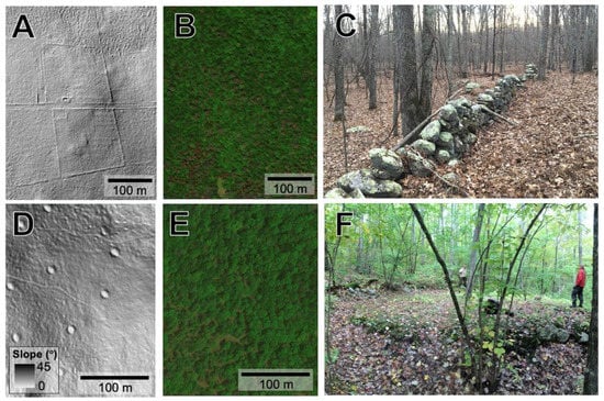
Figure 2.
(A,D) depict examples of extant historical land use features as seen in LiDAR DEM derivatives ((A) shows stone walls in a hillshaded DEM while (D) shows relict charcoal hearths in a slope raster). (B,E) depict current land cover (dense forest) in high-resolution aerial photography for those same extents, and (C,F) show examples of those feature types as they appear in the field.
Reconstructing historical forest cover and cleared land using historical land use features as a proxy has shown promise in several towns in Connecticut through comparison with improved and unimproved farmland recorded in the U.S. Census Nonpopulation Schedule for Agriculture [9]. Both stone walls and RCHs are reliable proxies in reconstructing areas of past land use and deforestation, specifically on smooth terrain that was cleared and used for agriculture, or rugged terrain which often remained forest was used specifically for harvesting timber, or used for charcoaling [9,20,34].
In this study, we demarcate and estimate areas of cleared and forested land based on extant historical land use features visible in LiDAR digital elevation models (DEMs) in several towns in Massachusetts to (1) determine the efficacy of methods published in [9] (which compared data from the 1850 U.S. Census Nonpopulation Schedule for Agriculture with LiDAR-derived estimates) on a broader scale in southern New England and the northeastern United States in general, and (2) assess the utility of other archival sources available in the region in comparison with LiDAR-derived estimates of cleared and forested land. Specifically, we compare areas with a high density of historical land use features indicative of deforestation which have been identified using LiDAR (stone walls and RCHs) with archival map data from 1830 and improved and unimproved land areas from the U.S. Census Nonpopulation Schedule for Agriculture from 1850, 1860, and 1870. This study builds on the novel approach outlined in [9] to reconstruct areas of historically cleared and forested land using extant historical land use features identified in airborne LiDAR data, and is applicable to other regions of the world where similar historic land use features and datasets exist. While modern land cover mapping has been undertaken in this region using airborne LiDAR [56], the methods presented here provide a unique approach to estimating and mapping areas of historical land cover. High-resolution regional historical forest cover estimates can provide an important complementary dataset for use in ongoing research to understand the impacts associated with the widespread historical deforestation that this region experienced in the 17th through 19th centuries and can be used in climate models, regional mapping programs, and can assist in other uses of modeling or quantifying impacts of historical deforestation.
2. Materials and Methods
2.1. Study Area
The study area encompasses 18 modern towns in Massachusetts (Figure 3, Table 1). To ensure consistency between areal estimates from the 19thcentury and present, we used an 1830 town boundary shapefile provided by Harvard Forest with their 1830 forest cover dataset [57] (see Section 2.3 for details) with which to compare modern town boundaries. For boundaries that did not match, we reviewed Massachusetts General Court records to determine which years the boundaries changed for that town [58]. We determined the state of all town boundaries in the year 1850, which is when the first agricultural census was conducted for each town, and then used a custom boundary shapefile for clipping LiDAR-derived data as well as forest data from the 1830 Harvard Forest shapefile (see Section 2.3 for details). For more information about specific town boundary changes, see Appendix A. Of note is that the modern towns of Adams and North Adams were one town (Adams) up until 1878, and for the purposes of this study, the area of both modern towns is combined in tables and calculations to represent the historical boundaries.
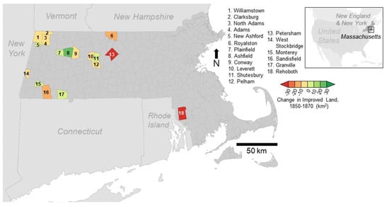
Figure 3.
Overview of study town locations in Massachusetts. Change in improved farmland (km2) from 1850 to 1870 is indicated for each town, compiled from U.S. Census Nonpopulation Schedule for Agriculture data [25,26]. Map projection is NAD 1983 UTM Zone 18N.

Table 1.
Overview of study towns, including data availability and characteristics of glacial deposits.
The majority of the towns are located in the central to western part of the state, where the bedrock geology is metamorphic schist and gneiss. Surficial deposits in these towns are primarily composed of lodgement and ablation till overlying bedrock (~75–100% of the town area; Table 1, see also Appendix C), with some fine to coarse glacial stratified (sand and gravel) deposits [61]. The exception is the town of Rehoboth, located in the southeastern corner of the state, where the bedrock geology is sedimentary rock, and is only covered by ~50% glacial till and ~40% glacial stratified deposits. Glacial till is the primary source of building material for stone walls [6,62]. The till varies in thickness from a few centimeters up to 60 m, and contains unsorted rock and mineral particles which are variable in distribution and range in size from clay to boulders [61]. Glacial stratified deposits primarily consist of clay to gravel sized sediment deposited by glacial meltwater [61]. Floodplain alluvium, a post-glacial deposit which generally overlies glacial stratified deposits, is located in river valleys and generally comprises less than 5–10% of the surficial deposits [61].
Some towns contain a higher percentage of post-glacial floodplain alluvium due to the presence of larger hydrological features. This includes the Hoosic River, which bisects Adams and North Adams and flows northward through Williamstown, becoming a tributary to the Hudson River in New York. The Williams River flows through West Stockbridge, eventually emptying into the Housatonic River. Rehoboth also contains a high percent of floodplain alluvium and swamp deposits due to its location within the Narragansett Bay watershed.
2.2. LiDAR Datasets, Feature Digitization, and Geospatial Analysis
While Massachusetts has full spatial coverage with LiDAR datasets currently, the datasets were collected separately over the course of several years (2002–2015) and therefore have slightly different characteristics [63]. Combined recent surveys undertaken between 2010 and 2015 provide high-resolution coverage for the entire state and have a nominal pulse spacing ranging from 0.35 to 2 m, with resulting digital elevation model (DEM) resolution of 1 and 2 m [63]. These datasets are publicly available via the Massachusetts Bureau of Geographic Information (MassGIS) OLIVER web mapping tool [64]. The specific datasets used in this study, 2015 Massachusetts (QL1), 2015 Massachusetts (QL2), 2013–2014 Sandy, and 2010 FEMA Narragansett, have a nominal pulse spacing ranging from 0.35 to 0.7 m. All of the datasets were collected by contractors working for federal agencies and using federal money; as a result, they are publicly available. The 2015 Massachusetts (QL1 and QL2) and 2013–2014 Sandy datasets were collected by contractors working for the United States Geological Survey (USGS), while the 2010 FEMA Narragansett dataset was collected by a contractor working for the Federal Emergency Management Agency (FEMA). All datasets were collected during leaf-off season in this region to obtain the most accurate measurements of the topography. The ability to accurately measure the ground surface is influenced not only by the presence of vegetation, but also by vegetation type [53,65]. The presence of coniferous vegetation, which retains its foliage year-round, can influence the number of LiDAR pulses that reach the actual ground surface in these areas [53]. Additionally, in forests with a dense understory, it is also challenging to discern the actual ground surface from low vegetation during point classification. In areas where pulses may not reach the ground surface as effectively, there may be fewer points to interpolate amongst during final DEM generation, making the morphology of fine-scale features in these areas somewhat less resolved [53,65]. The DEMs used in this study were generated by MassGIS from LAS 1.2 and 1.4 ground-classified points and have a 1 m pixel resolution [63]. All relevant tiles for each town were downloaded as DEMs from MassGIS OLIVER [64] and mosaicked using the Mosaic to New Raster tool in ArcMap.
Digitization of historical land use features from the DEMs was similar to the methods used and published in [9,44,62], in which features were manually identified using hillshade and slope rasters derived from the DEM in ArcMap using the Hillshade and Slope tools in the Spatial Analyst toolbox. Stone walls were digitized as polylines with vertices placed at intersections with other walls, changes in wall direction, and wall endpoints. A single point was placed in the center of each identified RCH. The stone wall and RCH datasets analyzed and included in this contribution were digitized by different users over the span of several years and then edited to maintain quality. Digitized datasets may have errors associated with LiDAR dataset quality (see [66] and above discussion) or user interpretation [67]. Experienced and novice mappers may consistently over- or under-map depending on their preferences and confidence in identifying features in a LiDAR DEM [67]. For stone walls in deciduous forests and relatively simple terrain, individual digitizers agreed with the group 88–92% of the time, but frequently missed walls, and on average, mapped only 78% of walls that were verified in the field [67]. These discrepancies increase in areas of coniferous forest, rugged terrain, or if topography has been modified by roads, buildings, or other infrastructure.
To derive areas representative of cleared and forested land, we used methods consistent with those published in [9] to generate rasters with the density of historical land use features, and then reclassify areas above specific density thresholds which are representative of intensive land use areas. Area was our preferred measurement in order to compare values with those recorded in the U.S. Census Nonpopulation Schedule for Agriculture, which recorded improved and unimproved farmland area. We first generated rasters depicting the density per km2 of the historical features, and then clipped those rasters to the town boundary. All rasters were generated using tools available from the ESRI ArcGIS suite using the arcpy library. Density rasters for stone walls were generated using the Line Statistics tool, and for RCHs using the Point Density tool, each with a circular neighborhood of 564.19 m for a resulting search area of 1 km2. The output rasters depicted the length of stone walls in km/km2 and the number of RCHs per km2. Consistent with the intensive land area threshold determination methods described in [9], we reclassified the stone wall density raster using the Reclassify tool so that areas where the length of stone walls exceeded 2 and 3 km/km2 were classified as improved (e.g., 2000.01–maximum = class 1) and the inverse areas were classified as unimproved (e.g., 0–2000 = class 0). For RCHs, we performed the same function for areas where RCH density exceeded 10 and 15 per km2 in order to compare our results to the previous study, which also used those thresholds. By reclassifying the rasters using this method, we captured areas of each town where land would have been used much more intensively for these specific land use types.
To determine the percentage of glacial till and other deposits for each town, a shapefile of Massachusetts surficial geology at the 1:250,000 scale [60] was used, and this layer was clipped to the extent of each town in the custom boundary shapefile and summarized by category of interest to determine the percent of town area for each deposit type. Higher resolution surficial maps exist for the state, however, at the town scale, the 1:250,000 resolution was sufficient for estimating the percent of the town surface area contributing to construction material for stone walls.
2.3. Archival Datasets
Two archival datasets were used in this study. The first was geospatial data of all woodland in the state in 1830, which was derived from a series of maps mandated of all towns by the Massachusetts legislature in 1830 [34,68,69]. The outcome of the mandate and subsequent survey was a map of almost every town in Massachusetts during the time period, variably showing forest, fields, buildings, roads, and other features of interest. While some maps were very detailed, others were not. Harvard Forest obtained these maps from a variety of archival locations and meticulously studied and digitized them. They subsequently made the digitized geospatial products available in 2009 through the Harvard Forest Digital Archive as downloadable geospatial data [57]. Scanned copies of most of these archival maps can now be accessed online [69]. The Harvard Forest dataset provides shapefiles of woodland, buildings, town boundaries, and other features derived from these maps for almost the entirety of Massachusetts in 1830 (Figure 4). The dataset description notes several limitations to the maps and thus geospatial data, including the fact that maps were generated by different individuals for each town and do not all conform to the same mapping standards. For example, in some towns, there are large generalized blocks of woodland, while in others, the areas are much more detailed, which could impact woodland estimates [57]. We do expect there to be some error associated with the calculated estimates we provide based on these maps (discussed in depth with results in Section 3); despite this, they do represent a valuable early resource in this region that is worth investigating and comparing to other potential historical land use estimates for this time period.
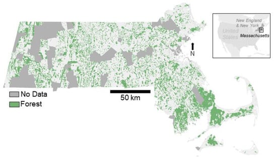
Figure 4.
1830 forest cover in Massachusetts from the Harvard Forest dataset digitized from 1830 archival maps [57] (also see [34], Figure 6 on p. 1327). Towns in dark gray do not have any data. Map projection is NAD 1983 UTM Zone 18N.
To calculate forested land from this dataset, the 1830lulc.shp file downloaded from the Harvard Forest Data Archive [57] was first edited to remove any polygons associated with towns denoted as missing woodland data. Next, we selected from the resulting layer any instances where the polygon attribute “WOODLAND” was 1, indicating that it had been classified as woodland. This selection was intersected with the custom town boundary shapefile described in Section 2.1 in order to calculate the amount of woodland for each town in the study using the Summary Statistics function. Using the Symmetrical Difference tool on the resulting layer allowed us to calculate areas of non-forested land in each study town, from which water that had been recorded in 1830 was removed using the Erase tool for polygons with a “LANDCOVER” class of 7 in the original 1830lulc.shp file.
The second archival dataset used was the U.S. Census Nonpopulation Schedule for Agriculture [30,70] (referred to throughout this text as ‘agricultural census’) for the years 1850, 1860, and 1870. The 1850 and 1860 agricultural censuses categorized farmland as ”Improved” and “Unimproved” land in acres for each farm in a town, whereas the 1870 agricultural census made a distinction between “Woodland” and “Other” as subsets within the “Unimproved” category. The instructions for the agricultural census defined unimproved land as “...a wood lot or other land at some distance but owned in connection with the farm, the timber or range of which is used for farm purposes...”, while improved land was defined as “...cleared and used for grazing, grass, or tillage, or which is now fallow” [71] (p. 235). We transcribed the values from the scanned ledgers of the 1850, 1860, and 1870 agricultural census available on Ancestry.com into tabular data, summed areas of “Improved” and “Unimproved” land for all recorded farms in the study towns, and then converted the acreages to km2 (1 acre = 4046.86 m2) [30].
We can expect small sources of error at the scale of this study with the use of historical census data for a variety of reasons, though studies have generally shown it to be reliable [9,72,73,74]. The most significant expected source of error is that often the sum of “Improved” and “Unimproved” areas is not equal to the total area of the town. The average percentage of town area covered by each agricultural census is as follows: 1850, 76%; 1860, 70%; 1870, 66%. The percentage of area comprised by both “Improved” and “Unimproved” land amongst towns varies drastically; in the 1850 census, percentages for the towns in this study range from 34% to 109%, for example. These variations could be a result of many factors, including that some farms were intentionally omitted by census-takers. The 1850 schedule itself notes that small farms with production value < USD 100 should not be included [71] (p. 235), a number which changed to USD 500 by 1870 [70]. A comparison of the population census for Clarksburg in 1850 against the agricultural census shows 42 male heads of household listed with the occupation of “Farmer,” yet only 32 of these men have farms listed in the agricultural census (~76%), and some men with other occupations (e.g., “Laborer”, “Manufacturer”) have farms noted in the agricultural census [30,75]. In addition to missing smaller farms, there were likely areas which were waterbodies, not farmland, and it is possible that some areas may have been left unenumerated or not visited. For example, the instructions for the agricultural census in 1870 specifically note “...Irreclaimable marshes and considerable bodies of water will be excluded in giving the area of a farm improved and unimproved” [71] (p. 746).
3. Results and Discussion
Overall, the density of stone walls varies throughout all of the study towns, with maximum densities within one individual town ranging from ~5 km/km2 in New Ashford to ~13 km/km2 in Royalston. All towns have minimum densities of 0 km/km2, as there are locations in all towns where no stone walls were digitized. Relict charcoal hearth (RCH) maximum densities range from 16 RCHs/km2 in Adams to 110 RCHs/km2 in Williamstown (Figure 5, Table 2). For comparison, towns in Connecticut that were analyzed and published in [9] had as many as 197 RCHs/km2 in some areas and stone wall length per km2 exceeding 11 km/km2. Therefore, it appears that while stone wall density is similar to that observed in Massachusetts, the area studied in Connecticut was used much more extensively for charcoal production.
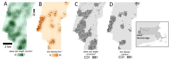
Figure 5.
Example showing stone wall (A) and relict charcoal hearth (RCH) (B) density in West Stockbridge, Massachusetts, and reclassified areas where stone wall length exceeds 2 km/km2 (C) and RCH density exceeds 10/km2 (D). Map projection is NAD 1983 UTM Zone 18N.
Table 2.
Maximum density values for stone walls and relict charcoal hearths (RCHs) in study towns.
By comparing the values of improved (i.e., non-forested) land area derived from the 1830 archival maps as well as 1850, 1860, and 1870 agricultural census records (Appendix B) with area values derived from LiDAR data (Table 3), we generally found that the areas in the 1830 maps have the highest correlation with estimates derived from the distribution of historical features in LiDAR data (R2 = 0.71), and of the agricultural census data values, those in 1850 have the highest correlation with LiDAR-derived area estimates (R2 = 0.57) (Figure 6).
Table 3.
Comparison of improved land area values (km2) for 1830, 1850, and LiDAR-derived data.
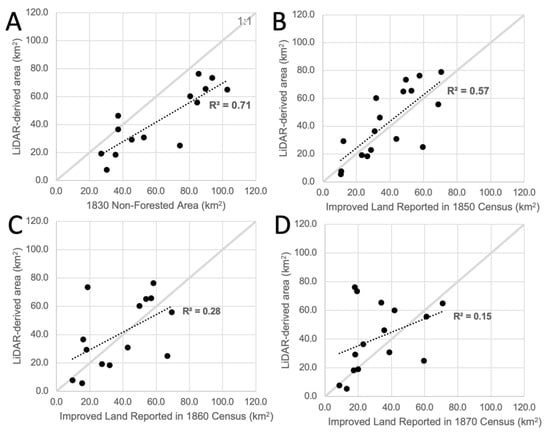
Figure 6.
Scatterplots showing the relationship between improved (i.e., non-forested) area from archival records and LiDAR-derived area where stone wall density is greater than 2 km/km2 in all study towns (black dots) for the years (A) 1830, (B) 1850, (C) 1860, and (D) 1870. Note that Monterey, Sandisfield, and Plainfield are not included in the 1860 plot (C), and Monterey and Sandisfield are not included in the 1870 plot (D). The boundaries of Monterey and Sandisfield changed after 1850, so their areas are not comparable, and Plainfield did not have agricultural census data available for 1860. The gray 1:1 line indicates the location where the estimated area from stone walls is equal to the value recorded in the agricultural census.
Combining the data from this study with five towns in Connecticut (see Figure 1) that were examined in a previous study [9] reveals a generally good correspondence (R2 = 0.70) between tabulated improved land in the 1850 agricultural census and areas of intensive land clearing derived from LiDAR data using a threshold where stone wall density exceeds 2 km/km2 (Figure 7). The trend (dotted line) also generally falls above the solid gray line that indicates a 1:1 agreement of values, suggesting that using this threshold slightly overestimates the amount of cleared land in a town in comparison to the census. In contrast with the results presented in Figure 8 of Reference [9], the correlation between 1850 agricultural data and areas derived from stone walls is not quite as strong in the subset of Massachusetts towns (R2 = 0.57, Figure 6B) as for the Connecticut towns (R2 = 0.97) [9]. There are several reasons this could be, including underlying surficial geology of the towns, and the timing of the historical peak of deforestation. We expect there will be more variation as more towns are included in the dataset, especially if towns are included which have lower proportions of glacial till, as there could be fewer stone walls there and higher proportions of wood historically used for fencing (see [6,8,76]).
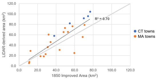
Figure 7.
LiDAR-derived area where stone wall length is >2 km/km2 plotted against areas of improved land in 1850 for Massachusetts (MA) and Connecticut (CT) towns combined. Data and plot for Connecticut towns are discussed in greater detail in [9,62]. The gray 1:1 line indicates the location where the estimated area from stone walls is equal to the value recorded in the agricultural census.
This method of determining cleared or forested land using stone walls as a proxy appears to work more effectively in towns comprised almost solely of glacial till. This would have provided farmers a means to construct walls throughout the entire town without areas of constraint depending on the surficial materials. For example, within the plots of Figure 6, we observed several towns that fall well below a 1:1 agreement, indicating that our methods underestimate the amount of cleared land that was recorded in these towns. This may be influenced by the presence of riverine or glacial lake deposits, which would result in fewer stone walls than expected in these towns. The 1850 agricultural census values appear to be a slightly better fit with estimates from LiDAR data, as our method seems to underestimate the amount of non-forested land in almost every town in 1830 (Figure 6A). In the 1850 agricultural census plot (Figure 6B), towns that fall below the 1:1 line, such as Adams, Conway, Leverett, Williamstown, and West Stockbridge, are comprised of a much higher proportion of floodplain alluvium, sand, and gravel than other towns in the study area (see Appendix C). All of these towns therefore likely contain large areas which may have been deforested or fenced, but do not have any stone walls demarcating those events given the lack of stone fencing material. It is likely that other types of fencing were used in these towns to demarcate cleared land, notably in the general area of the former glacial Lake Hitchcock and current Hoosic River watersheds. This is not unexpected, as it has been shown that surficial materials, notably glacial till, influence the presence, type, and morphology of stone walls [6,62]. It appears, therefore, that in towns where there is less glacial till and more sand or glacial lake deposits, the method does not appear to work as well, and this may be why there is such variation in Massachusetts compared with the five towns that were studied in Connecticut. In Connecticut, the towns that were studied also had extensive spatial coverage with both stone walls and RCHs, which allowed for a nearly complete sampling of space in each town. This likely contributed to the accuracy of the LiDAR-derived estimates. In Massachusetts, there are large areas of each town that are not covered by stone walls or RCHs, which leaves these areas effectively unsampled and unknown.
We hypothesize that another reason the correlation between the map or agricultural census data and the LiDAR-derived area estimates is not as strong for the Massachusetts towns could be because the height of land clearance in Massachusetts was not in 1830, or even 1850 as it was in Connecticut, but later in the 19th century, as shown in other studies [12,77,78]. For example, Foster [77] provides forest data for Petersham with a height of clearance in 1860, and for Conway/Shelburne [79], where the height of clearance was ca. 1840–1860. Despite this, comparison of LiDAR-derived areas with totals from agricultural census records from 1860 and 1870 have an even weaker correlation (Figure 6C,D) with our estimates, suggesting that 1850 continues to provide the likely peak of deforestation for this particular group of towns on average. While Monterey and Sandisfield are not included in the 1870 plot, and those towns plus Plainfield are not included in the 1860 plot, removal of all three towns from the 1850 plot, which has the best correlation, shows it decreases to R2 = 0.50, suggesting that this year still has the best outcome of the agricultural census values. With regard to timing and spatial distribution, it appears that the extant stone walls on the landscape are representative of all land that had ever been cleared in the town, assuming stone fencing had been used. We observe this when comparing stone wall area estimates to agricultural census estimates from time periods known to have been the height of agricultural clearance, and this is also likely why our method underestimates the 1830 values. Comparing LiDAR-derived estimates to census-derived estimates for 1850, 1860, and 1870 reveals this quite clearly.
We also found that in Massachusetts towns such as West Stockbridge, where charcoaling seems to have occurred on a fairly widespread scale, the location of RCHs corresponds well to areas demarcated as being forest during 1830, and we can infer that those areas would have also been deforested at some point in time (Figure 8). As demonstrated in [9], rugged terrain unfit for agriculture was typically used for charcoaling during the 19th century, and these areas also correspond well to areas marked “Unimproved” in agricultural census records. However, charcoaling did not occur as frequently in some of the towns as in others, likely due to a variety of factors, including proximity to iron furnaces or ease of transport.
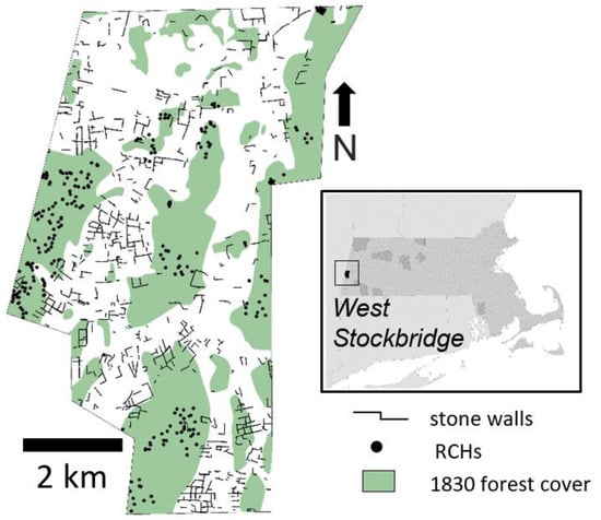
Figure 8.
Relict charcoal hearths (RCHs) tend to occur in areas of towns which were typically not well-suited for agriculture, as shown here in West Stockbridge, Massachusetts, where RCHs occur in areas of the town which were forested in 1830. Map projection is NAD 1983 UTM Zone 18N.
While the 1830 maps provide an unprecedented view of forest cover in Massachusetts during this time period, there is also error associated with them. Harvard Forest makes note of several data usage caveats in their dataset description, including that the maps were drafted by different individuals and there was no standardized cartographic approach. Additionally, it has now been almost twenty years since these maps were digitized by Harvard Forest, and it is possible that updates to GIS software could provide slightly different results. As an example of error in this dataset, see Figure 9, which depicts the eastern extent of Clarksburg, where the 19th century surveyor likely meant to include all of the mountainous area in their forested extent, but when the map is georeferenced and overlaid on a LiDAR DEM (Figure 9B), the forested extent only accounts for a small portion of the actual mountainous terrain, and does in fact match fairly closely with the data from Harvard Forest’s digitized shapefile (Figure 9C). It is possible that a comprehensive comparison of the forest dataset with high-resolution LiDAR DEMs could potentially provide more accurate estimates.
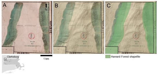
Figure 9.
Panels (A) through (C) show the same extent of the eastern portion of Clarksburg, Massachusetts: (A) is the archival 1830 map (Public Domain, [80]) showing forest covering mountainous areas, (B) shows that map georeferenced and overlaid with 30% transparency on a LiDAR DEM, and (C) shows (B) plus the current extent of digitized forest cover from the Harvard Forest dataset which was digitized from the same map in the early 2000s. Map projection is NAD 1983 UTM Zone 18N.
4. Conclusions
In general, this work demonstrated that features representative of historical deforestation identified in LiDAR data can be reliably used as a proxy to estimate areas and the spatial extents of cleared and forested land in Massachusetts and elsewhere in the northeastern United States. As feature digitization continues, expanding the ability to estimate areas of deforested and forested land will broaden and become more feasible. We found that there is spatial variation amongst the towns regionally in terms of the density of extant relict land use features (i.e., stone walls and RCHs), and thus the overall ability to reconstruct areas of possible improved (i.e., deforested or cleared) land. In areas where stone might have been less available for wall building and where fencing might have been comprised partially or entirely of wood, it is also much more challenging to reconstruct areas that might have been improved, and vice versa. The same is true if stone walls have been removed or are otherwise no longer preserved or visible on the land surface. While there are some limitations with archival data, when combined with airborne LiDAR, these resources help confirm that extant historical land use features identified using LiDAR data can be used to reliably reconstruct deforested areas on regional scales.
Overall, the impacts of historical deforestation in this region were significant, and this is evident from the widespread relict land use features visible across the landscape. Continued research to understand and quantify these impacts in the northeastern U.S. is important in understanding past, present, and future aspects of forest ecology, climate, wildlife biology, geomorphology, and a range of other considerations. Recent efforts to automate digitization of these historical land use features will allow for expansion of these methods across regional scales and provide high-resolution historical land cover estimates to assist in understanding these impacts.
Author Contributions
Conceptualization, K.M.J. and W.B.O.; methodology, K.M.J. and W.B.O.; validation, K.M.J., W.B.O. and S.D.; formal analysis, K.M.J., W.B.O., S.D. and C.H.; dataset development: K.M.J., W.B.O., S.D. and C.H., also see acknowledgements; writing—original draft preparation, K.M.J., W.B.O. and S.D.; writing—review and editing, K.M.J., W.B.O., S.D. and C.H.; funding acquisition, W.B.O. and the Cooperative Institute for Satellite Earth System Studies (CISESS). All authors have read and agreed to the published version of the manuscript.
Funding
This work was partially funded by National Science Foundation grant BCS-1654462 to W. Ouimet, and partially supported by the National Oceanic and Atmospheric Administration through the Cooperative Institute for Satellite Earth System Studies under Cooperative Agreement NA19NES4320002.
Data Availability Statement
The LiDAR datasets used in this study are free and publicly available via MassGIS OLIVER (see references). The custom town boundary shapefile was generated using the town boundary information in Appendix A and the Town Boundary shapefile for towns of Massachusetts available at MassGIS. The archival data for 1830 woodland were obtained from Harvard Forest (see references). The archival data for the 1850, 1860, and 1870 agricultural census used in this study are provided in Appendix B, with the original un-transcribed data available with an Ancestry.com subscription at https://www.ancestry.com/search/collections/1276/ (accessed on 6 September 2021). Digitized historical land use features are available at the following ArcGIS Online maps: (1) stone walls: https://connecticut.maps.arcgis.com/apps/webappviewer/index.html?id=0208461aa98a4df3969624e7110e1f2c (accessed on 6 September 2021), and (2) RCHs: https://www.arcgis.com/apps/webappviewer/index.html?id=102f6831a12843878ea8081aec41029d (accessed on 6 September 2021).
Acknowledgments
In addition to the authors, the following individuals contributed digitized datasets of stone walls and relict charcoal hearths used in this study: Eli Anderson, Max Fortin, Matt Fryer, and students in the University of Massachusetts Introduction to GIS class in the Department of Geography taught by Forrest J. Bowlick.
Conflicts of Interest
The authors declare no conflict of interest. The funders had no role in the design of the study; in the collection, analyses, or interpretation of data; in the writing of the manuscript, or in the decision to publish the results.
Appendix A
Town Boundary Details
Adams and North Adams are today separate towns, but were the same town up until 1878; for the purposes of this study, the two modern towns were recombined and are referred to as “Adams” throughout the text. Additionally, in 1900, the boundary between North Adams and Williamstown was slightly modified to its present state [81]. Clarksburg lost its easternmost portion to the town of Florida in 1913 [82]. A small portion (~2 km2) of Conway’s NW corner was annexed to Buckland, an adjacent town, in 1838 [83]. Monterey was part of the town of Tyringham until 1847 when it split off, and subsequently gained more land from adjacent New Marlborough in 1851 [84] and Sandisfield in 1875 [85]. Sandisfield itself lost a different tract of land to nearby Tolland in 1853 [86]. Petersham’s southern boundary was expanded in the 1930s as a result of the construction of the Quabbin Reservoir. The reservoir covers, either partially or fully, four historical towns, which were disincorporated and flooded for the reservoir’s construction, and associated land was ceded to adjacent extant towns. Two of the disincorporated towns, Dana and Greenwich, are mostly encompassed by Petersham’s modern boundaries today. Most of Petersham’s original boundaries were not subject to flooding for the reservoir’s construction, with the exception of a small piece in the west, which appears to have been a low marshy forested area in 1830 according to the maps used in this study. Petersham’s land use history has been thoroughly studied and meticulously documented by researchers at Harvard Forest, which is located there. For more about impacts of historical land use on forest composition, ecology, and other factors, see the following for some examples: [80,87]. West Stockbridge’s boundary was changed slightly in 1847 when part of the town was annexed by an adjacent town (Alford) [88].
Appendix B
Table A1.
Improved and unimproved land for 1850, 1860, and 1870 from the U.S. Census Nonpopulation Schedule for Agriculture.
Table A1.
Improved and unimproved land for 1850, 1860, and 1870 from the U.S. Census Nonpopulation Schedule for Agriculture.
| Town | Improved Land (km2), 1850 | Unimproved Land (km2), 1850 | Improved Land (km2), 1860 | Unimproved Land (km2), 1860 | Improved Land (km2), 1870 | Unimproved Land (km2), 1870 |
|---|---|---|---|---|---|---|
| Adams | 43.8 | 38.0 | 42.8 | 42.8 | 38.8 | 33.7 |
| Ashfield | 48 | 33.2 | 53.8 | 53.8 | 70.8 | 22.2 |
| Clarksburg | 10.9 | 25.3 | 9.6 | 9.6 | 8.7 | 9.6 |
| Conway | 68.7 | 17.9 | 69.3 | 69.3 | 61.2 | 10.4 |
| Granville | 31.9 | 36.8 | 50 | 50.0 | 41.8 | 44.9 |
| Leverett | 26.5 | 20.4 | 32 | 32.0 | 17.3 | 20.2 |
| Monterey | 28.6 | 12.9 | 21.3 | 21.3 | 28.7 | 22.9 |
| New Ashford | 10.8 | 6.5 | 15.4 | 15.4 | 13.2 | 9.4 |
| Pelham | 30.8 | 12.9 | 16.1 | 16.1 | 23 | 8.9 |
| Petersham | 57.7 | 22.5 | 58.4 | 58.4 | 17.9 | 6.8 |
| Plainfield | 33.9 | 16.6 | - | - | 35.6 | 12.4 |
| Rehoboth | 49.6 | 43.7 | 18.6 | 18.6 | 19.4 | 23.0 |
| Royalston | 52.7 | 33.3 | 56.9 | 56.9 | 34 | 17.4 |
| Sandisfield | 70.5 | 37.1 | 92.6 | 92.6 | 57.3 | 34.7 |
| Shutesbury | 12.2 | 11.6 | 18 | 18.0 | 18.1 | 26.2 |
| W. Stockbridge | 23.2 | 10.4 | 27.4 | 27.4 | 20 | 7.3 |
| Williamstown | 59.6 | 28.3 | 66.8 | 66.8 | 59.5 | 25.7 |
Appendix C
Table A2.
Percent of town area covered by surficial deposits.
Table A2.
Percent of town area covered by surficial deposits.
| Town | Till (%) | Glacial Stratified Sand and Gravel (%) | Floodplain Alluvium (%) |
|---|---|---|---|
| Adams | 85.9 | 9.0 | 5.1 |
| Ashfield | 90.9 | 8.3 | 0.8 |
| Clarksburg | 93.4 | 6.2 | 0.4 |
| Conway | 89.9 | 9.0 | 1.2 |
| Granville | 92.7 | 6.8 | 0.5 |
| Leverett | 77.2 | 22.0 | 0.8 |
| Monterey | 94.4 | 5.2 | 0.4 |
| New Ashford | 98.5 | 1.4 | 0 |
| Pelham | 87.8 | 12.2 | 0 |
| Petersham | 88.6 | 10.5 | 0.9 |
| Plainfield | 99.8 | 0.2 | 0 |
| Rehoboth | 49.6 | 41.1 | 9.3 |
| Royalston | 83.8 | 11.3 | 4.9 |
| Sandisfield | 96.5 | 2.6 | 0.9 |
| Shutesbury | 81.0 | 18.5 | 0.5 |
| W. Stockbridge | 82.1 | 12.5 | 5.4 |
| Williamstown | 78.3 | 16.5 | 3.3 |
References
- Bernstein, D.J. Long-term continuity in the archaeological record from the coast of New York and southern new England, USA. J. Isl. Coast. Archaeol. 2006, 1, 271–284. [Google Scholar] [CrossRef]
- Chapdelaine, C.; Boisvert, R.A.; Ellis, C.J.; Bradley, J.W.; Crock, J.G.; Robinson, F.W.; Lothrop, J.C.; Bradley, J.W. Late Pleistocene Archaeology and Ecology in the Far Northeast; A&M University Press: College Station, TX, USA, 2012; ISBN 9781603448055. [Google Scholar]
- Cronon, W. Changes in the Land; Hill and Wang: New York, NY, USA, 1983. [Google Scholar]
- Lothrop, J.C.; Newby, P.E.; Spiess, A.E.; Bradley, J.W. Paleoindians and the Younger Dryas in the New England-Maritimes Region. Quat. Int. 2011, 242, 546–569. [Google Scholar] [CrossRef]
- Donahue, B. The Great Meadow: Farmers and the Land in Colonial Concord; Yale University Press: New Haven, CT, USA, 2004. [Google Scholar]
- Thorson, R.M. Stone by Stone: The Magnificent History in New England’s Stone Walls; Walker & Company: New York, NY, USA, 2002. [Google Scholar]
- Ridge, J.C. The Quaternary glaciation of western New England with correlations to surrounding areas. Dev. Quat. Sci. 2004, 2, 169–199. [Google Scholar]
- Dodge, J.R. Statistics of Fences in the United States. In Report of the Commissioner of Agriculture for the Year 1871; Dodge, J.R., Ed.; United States Department of Agriculture, Government Printing Office: Washington, DC, USA, 1872; pp. 497–512. [Google Scholar]
- Johnson, K.M.; Ouimet, W.B. Reconstructing Historical Forest Cover and Land Use Dynamics in the Northeastern United States Using Geospatial Analysis and Airborne LiDAR. Ann. Am. Assoc. Geogr. 2021, 111, 1656–1678. [Google Scholar] [CrossRef]
- Ives, T.H. Cairnfields in New England’s Forgotten Pastures. Archaeol. East. N. Am. 2015, 43, 119–132. [Google Scholar]
- Allport, S. Sermons in Stone: The Stone Walls of New England and New York; W.W. Norton & Company: New York, NY, USA, 1990. [Google Scholar]
- Foster, D.R. Land-Use History (1730–1990) and Vegetation Dynamics in Central New England, USA. J. Ecol. 1992, 80, 753. [Google Scholar] [CrossRef]
- Burakowski, E.A.; Ollinger, S.V.; Bonan, G.B.; Wake, C.P.; Dibb, J.E.; Hollinger, D.Y. Evaluating the climate effects of reforestation in New England using a weather research and forecasting (WRF) model multiphysics ensemble. J. Clim. 2016, 29, 5141–5156. [Google Scholar] [CrossRef]
- Hill, M.M. Gully Erosion and Holocene-Anthropocene Environmental Change in southern New England. Ph.D. Thesis, University of Connecticut, Storrs, CT, USA, 2019. [Google Scholar]
- Gordon, R.B.; Raber, M. Industrial Heritage in Northwest Connecticut; Connecticut Academy of Arts and Sciences: New Haven, CT, USA, 2000. [Google Scholar]
- Straka, T.J. Historic Charcoal Production in the US and Forest Depletion: Development of Production Parameters. Adv. Hist. Stud. 2014, 3, 104–114. [Google Scholar] [CrossRef][Green Version]
- Knowles, A.K. Mastering Iron: The Struggle to Modernize an American Industry, 1800–1868; University of Chicago Press: Chicago, IL, USA, 2013. [Google Scholar]
- Bonhôte, J.; Davasse, B.; Dubois, C.; Isard, V.; Métailié, J.-P. Charcoal kilns and environmental history in the eastern Pyrenees (France). A methodological approach. In Charcoal Analysis: Methodological Approaches, Palaeoecological Results and Wood Uses, Proceedings of the Second International Meeting of Anthracology, Paris, France, September 2000; Thiebault, S., Ed.; Archaeopress: Oxford, UK, 2002; pp. 219–228. [Google Scholar]
- Carter, B.P. Identifying Landscape Modification using Open Data and Tools: The Charcoal Hearths of the Blue Mountain, Pennsylvania. Hist. Archaeol. 2019, 53, 432–443. [Google Scholar] [CrossRef]
- Carter, B.P.; Blackadar, J.H.; Conner, W.L.A. When Computers Dream of Charcoal: Using Deep Learning, Open Tools, and Open Data to Identify Relict Charcoal Hearths in and around State Game Lands in Pennsylvania. Adv. Archaeol. Pract. 2021, 1–15. [Google Scholar] [CrossRef]
- Hesse, R. Charcoal burning platforms in the southern Black Forest: From LIDAR point cloud to spatial patterns of resource use. Poster Presented at the International Open Workshop: Socio-Environmental Dynamics over the Last 12,000 Years: The Creation of Landscapes III, Kiel University, Germany, 15–18 April 2013; Kiel University: Kiel, Germany, 2013. [Google Scholar]
- Potter, N.J.; Brubaker, K.M.; Delano, H. LiDAR Reveals Thousands of 18th and 19th Century Charcoal Hearths on South Mountain, South-Central Pennsylvania. GSA Abstr. Programs 2013, 45, 99. [Google Scholar]
- Raab, T.; Hirsch, F.; Ouimet, W.; Johnson, K.M.; Dethier, D.; Raab, A. Architecture of relict charcoal hearths in northwestern Connecticut, USA. Geoarchaeology 2017, 32, 502–510. [Google Scholar] [CrossRef]
- Raab, A.; Takla, M.; Raab, T.; Nicolay, A.; Schneider, A.; Rösler, H.; Heußner, K.U.; Bönisch, E. Pre-industrial charcoal production in Lower Lusatia (Brandenburg, Germany): Detection and evaluation of a large charcoal-burning field by combining archaeological studies, GIS-based analyses of shaded-relief maps and dendrochronological age determination. Quat. Int. 2015, 367, 111–122. [Google Scholar] [CrossRef]
- Barger, L.C. Life on a Rocky Farm: Rural Life near New York City in the Late Nineteenth Century; Rogerson, P.A., Ed.; University of New York Press: Albany, NY, USA, 2013. [Google Scholar]
- Foster, D.R.; Aber, J.D. Forests in Time: The Environmental Consequences of 1000 Years of Change in New England; Yale University Press: New Haven, CT, USA, 2004. [Google Scholar]
- Bell, M.M. The Face of Connecticut; State Geological and Natural History Survey of Connecticut: Hartford, CT, USA, 1985. [Google Scholar]
- Foster, D.R. Thoreau’s country: A historical-ecological perspective on conservation in the New England landscape. J. Biogeogr. 2002, 29, 1537–1555. [Google Scholar] [CrossRef]
- Manson, S.; Schroeder, J.; Van Riper, D.; Kugler, T.; Ruggles, S. IPUMS National Historical Geographic Information System: Version 16.0; IPUMS: Minneapolis, MN, USA, 2021. [Google Scholar] [CrossRef]
- Ancestry.com U.S. Selected Federal Census Non-Population Schedules, 1850–1880; Ancestry.com Operations, Inc.: Provo, UT, USA, 2010; Available online: https://www.ancestry.com/search/collections/1276/ (accessed on 6 September 2021).
- Moser, W.K.; Butler-Leopold, P.; Hausman, C.; Iverson, L.; Ontl, T.; Brandt, L.; Matthews, S.; Peters, M.; Prasad, A. The Impact of Climate Change on Forest Systems in the Northern United States: Projections and Implications for Forest Management. In Achieving Sustainable Management of Boreal and Temperate Forests; Stanurf, J.A., Ed.; Burleigh Dodds Science Publishing Limited: Cambridge, UK, 2019; pp. 1–50. ISBN 9781786762924. [Google Scholar]
- Francis, D.R.; Foster, D.R. Response of small New England ponds to historic land use. Holocene 2001, 11, 301–312. [Google Scholar] [CrossRef]
- D’Amato, A.W.; Orwig, D.A.; Foster, D.R. New estimates of Massachusetts old-growth forests: Useful data for regional conservation and forest reserve planning. Northeast. Nat. 2006, 13, 495–506. [Google Scholar] [CrossRef]
- Hall, B.; Motzkin, G.; Foster, D.R.; Syfert, M.; Burk, J. Three hundred years of forest and land-use change in Massachusetts, USA. J. Biogeogr. 2002, 29, 1319–1335. [Google Scholar] [CrossRef]
- Foster, D.R.; Motzkin, G.; Slater, B. Land-Use History as Long-Term Broad-Scale Disturbance: Regional Forest Dynamics in Central New England. Ecosystems 1998, 1, 96–119. [Google Scholar] [CrossRef]
- Thorson, R.M.; Harris, A.G.; Harris, S.L.; Gradie, R.I.; Lefor, M.W. Colonial impacts to wetlands in Lebanon, Connecticut. Rev. Eng. Geol. 1998, 12, 23–42. [Google Scholar]
- Thorson, R.M.; Harris, S.L. How “Natural” Are Inland Wetlands? An Example From the Trail Wood Audubon Sanctuary in Connecticut, USA. Environ. Manag. 1991, 15, 675–687. [Google Scholar] [CrossRef]
- Walter, R.C.; Merritts, D.J. Natural streams and the legacy of water-powered mills. Science 2008, 319, 299–304. [Google Scholar] [CrossRef]
- Mayer, A.E.G.; McGreevy, T.J., Jr.; Sullivan, M.E.; Buffum, B.; Husband, T.P. Fine-Scale Habitat Comparison of Two Sympatric Cottontail Species in Eastern Connecticut. Curr. Trends For. Res. 2018, 2018, 1–8. [Google Scholar]
- Chase, A.F.; Chase, D.Z.; Fisher, C.T.; Leisz, S.J.; Weishampel, J.F. Geospatial revolution and remote sensing LiDAR in Mesoamerican archaeology. Proc. Natl. Acad. Sci. USA 2012, 109, 12916–12921. [Google Scholar] [CrossRef] [PubMed]
- Davis, D.S.; Sanger, M.C.; Lipo, C.P. Automated mound detection using lidar and object-based image analysis in Beaufort County, South Carolina. Southeast. Archaeol. 2019, 38, 23–37. [Google Scholar] [CrossRef]
- Devereux, B.J.; Amable, G.S.; Crow, P.; Cliff, A.D. The potential of airborne lidar for detection of archaeological features under woodland canopies. Antiquity 2005, 78, 648–660. [Google Scholar] [CrossRef]
- Doneus, M.; Briese, C. Full-waveform airborne laser scanning as a tool for archaeological reconnaissance. In From Space to Place: 2nd International Conference on Remote Sensing in Archaeology, Proceedings of the 2nd International Workshop, CNR, Rome, Italy, 4–7 December 2006; Campana, S., Forte, M., Eds.; BAR Publishing: Oxford, UK, 2006; pp. 99–106. [Google Scholar]
- Johnson, K.M.; Ouimet, W.B. Rediscovering the lost archaeological landscape of southern New England using airborne light detection and ranging (LiDAR). J. Archaeol. Sci. 2014, 43, 9–20. [Google Scholar] [CrossRef]
- Bewley, R.H.; Crutchley, S.P.; Shell, C.A. New light on an ancient landscape: Lidar survey in the Stonehenge world heritage site. Antiquity 2005, 79, 636–647. [Google Scholar] [CrossRef]
- Gallagher, J.M.; Josephs, R.L. Using LiDAR to Detect Cultural Resources in a Forest Environment: An Example from Isle Royale National Park, Michigan, USA. Archaeol. Prospect. 2008, 15, 187–206. [Google Scholar] [CrossRef]
- Evans, D. Airborne laser scanning as a method for exploring long-term socio-ecological dynamics in Cambodia. J. Archaeol. Sci. 2016, 74, 164–175. [Google Scholar] [CrossRef]
- Affek, A.N.; Wolski, J.; Latocha, A.; Zachwatowicz, M.; Wieczorek, M. The use of LiDAR in reconstructing the pre-World War II landscapes of abandoned mountain villages in southern Poland. Archaeol. Prospect. 2021, 1–17. [Google Scholar] [CrossRef]
- Bennett, R.; Welham, K.; Hill, R.A.; Ford, A. A Comparison of Visualization Techniques for Models Created from Airborne Laser Scanned Data. Archaeol. Prospect. 2012, 19, 41–48. [Google Scholar] [CrossRef]
- Štular, B.; Kokalj, Ž.; Oštir, K.; Nuninger, L. Visualization of lidar-derived relief models for detection of archaeological features. J. Archaeol. Sci. 2012, 39, 3354–3360. [Google Scholar] [CrossRef]
- Schindling, J.; Gibbes, C. LiDAR as a tool for archaeological research: A case study. Archaeol. Anthropol. Sci. 2014, 6, 411–423. [Google Scholar] [CrossRef]
- Beach, T.; Luzzadder-Beach, S.; Krause, S.; Guderjan, T.; Valdez, F.; Fernandez-Diaz, J.C.; Eshleman, S.; Doyle, C. Ancient Maya wetland fields revealed under tropical forest canopy from laser scanning and multiproxy evidence. Proc. Natl. Acad. Sci. USA 2019, 116, 21469–21477. [Google Scholar] [CrossRef]
- Johnson, K.M.; Ouimet, W.B. An observational and theoretical framework for interpreting the landscape palimpsest through airborne LiDAR. Appl. Geogr. 2018, 91, 32–44. [Google Scholar] [CrossRef]
- Mlekuž, D. Messy Landscapes: Lidar and The Practices of Landscaping. In Interpreting Archaeological Topography: Lasers, 3D Data, Observation, Visualisation and Applications; Opitz, R.S., Cowley, D.C., Eds.; Oxbow Books: Oxford, UK, 2013; pp. 90–101. [Google Scholar]
- Bailey, G. Time perspectives, palimpsests and the archaeology of time. J. Anthropol. Archaeol. 2007, 26, 198–223. [Google Scholar] [CrossRef]
- Parent, J.R.; Volin, J.C.; Civco, D.L. A fully-automated approach to land cover mapping with airborne LiDAR and high resolution multispectral imagery in a forested suburban landscape. ISPRS J. Photogramm. Remote Sens. 2015, 104, 18–29. [Google Scholar] [CrossRef]
- Foster, D.R.; Motzkin, G. 1830 Map of Land Cover and Cultural Features in Massachusetts. Harvard Forest Data Archive: HF122 (v.15). Available online: https://harvardforest1.fas.harvard.edu/exist/apps/datasets/showData.html?id=hf122 (accessed on 22 October 2021).
- State Library of Massachusetts Acts and Resolves. Available online: https://archives.lib.state.ma.us/handle/123456789/2 (accessed on 9 October 2021).
- Secretary of the Commonwealth of Massachusetts Massachusetts City and Town Incorporation and Settlement Dates. Available online: https://www.sec.state.ma.us/cis/cisctlist/ctlistalph.htm (accessed on 6 September 2021).
- Massachusetts Bureau of Geographic Information (MassGIS) MassGIS Data: Surficial Geology (1:250,000). Available online: https://www.mass.gov/info-details/massgis-data-surficial-geology-1250000 (accessed on 6 September 2021).
- Stone, J.R.; Stone, B.D.; DiGiacomo-Cohen, M.L.; Mabee, S.B. Surficial Materials of Massachusetts—A 1:24,000-Scale Geologic Map Database U.S. Geological Survey Scientific Investigations Map 3402; U.S. Geological Survey: Reston, VA, USA, 2018.
- Johnson, K.M.; Ouimet, W.B. Physical properties and spatial controls of stone walls in the northeastern USA: Implications for Anthropocene studies of 17th to early 20th century agriculture. Anthropocene 2016, 15, 22–36. [Google Scholar] [CrossRef]
- Massachusetts Bureau of Geographic Information (MassGIS) MassGIS Data: LiDAR Terrain Data. Available online: https://www.mass.gov/info-details/massgis-data-lidar-terrain-data (accessed on 9 October 2021).
- Massachusetts Bureau of Geographic Information (MassGIS) OLIVER: MassGIS’s Online Mapping Tool. Available online: http://maps.massgis.state.ma.us/map_ol/oliver.php (accessed on 9 October 2021).
- Doneus, M.; Briese, C.; Fera, M.; Janner, M. Archaeological prospection of forested areas using full-waveform airborne laser scanning. J. Archaeol. Sci. 2008, 35, 882–893. [Google Scholar] [CrossRef]
- Johnson, K.M.; Ives, T.H.; Ouimet, W.B.; Sportman, S.P. High-resolution airborne Light Detection and Ranging data, ethics and archaeology: Considerations from the northeastern United States. Archaeol. Prospect. 2021, 28, 293–303. [Google Scholar] [CrossRef]
- Leonard, J.; Ouimet, W.B.; Dow, S. Evaluating User Interpretation and Error associated with Digitizing Stone Walls using airborne LiDAR. Geol. Soc. Am. Abstr. Programs 2021, 53. [Google Scholar] [CrossRef]
- Massachusetts General Court House of Representatives 1830 House Bill 0037. Report of the Select Committee Appointed to Consider the Expediency of Procuring a Map of the Commonwealth, Including Multiple Resolves. Available online: https://archives.lib.state.ma.us/handle/2452/820196 (accessed on 9 October 2021).
- Digital Commonwealth Massachusetts State Archives: Town Plans. 1830. Available online: https://www.digitalcommonwealth.org/search?f%5Bcollection_name_ssim%5D%5B%5D=Town+plans%2C+1830&f%5Binstitution_name_ssim%5D%5B%5D=Massachusetts+Archives&f%5Brelated_item_series_ssim%5D%5B%5D=Town+plans%2C+1830&only_path=true (accessed on 9 October 2021).
- National Archives Nonpopulation Census Records. Available online: https://www.archives.gov/research/census/nonpopulation (accessed on 6 September 2021).
- Wright, C.D.; Hunt, W.C. The History and Growth of the United States Census; U.S. Government Printing Office: Washington, DC, USA, 1900.
- Ginsberg, C.A. Estimates and Correlates of Enumeration Completeness: Censuses and Maps in Nineteenth-Century Massachusetts. Soc. Sci. Hist. 1988, 12, 71–86. [Google Scholar] [CrossRef]
- Steckel, R.H. The Quality of Census Data for Historical Inquiry: A Research Agenda. Soc. Sci. Hist. 1991, 15, 579–599. [Google Scholar] [CrossRef]
- Parkerson, D.H. Comments on the Underenumeration of the U.S. Census, 1850–1880. Sci. Hist. 1991, 15, 509–515. [Google Scholar]
- Ancestry.com. 1850 United States Federal Census; Ancestry.com Operations, Inc.: Lehi, UT, USA, 2009; Available online: https://www.ancestry.com/search/collections/8054/ (accessed on 9 October 2021).
- Thorson, R.M. Exploring Stone Walls: A Field Guide to New England’s Stone Walls; Walker & Company: New York, NY, USA, 2005. [Google Scholar]
- Foster, D.R.; Zebryk, T.; Schoonmaker, P.; Lezberg, A. Post-Settlement History of Human Land-Use and Vegetation Dynamics of a Tsuga Canadensis (Hemlock) Woodlot in Central New England. J. Ecol. 1992, 80, 773. [Google Scholar] [CrossRef]
- Foster, D.R.; Donahue, B.; Kittredge, D.; Motzkin, G.; Hall, B.; Turner, B.; Chilton, E.S. New England’s Forest Landscape: Ecological Legacies and Conservation Patterns Shaped by Agrarian History. In Agrarian Landscapes in Transition: Comparisons of Long-Term Ecological & Cultural Change; Redman, C.L., Foster, D.R., Eds.; Oxford University Press: Oxford, UK, 2008; pp. 44–88. [Google Scholar]
- Motzkin, G.; Bellemare, J.; Foster David, R. Legacies of the agricultural past in the forested present: An assessment of historical land-use effects on Rich Mesic Forests. J. Biogeogr. 2002, 29, 1401–1420. [Google Scholar]
- Massachusetts Archives Plan of Clarksburg, Surveyor’s Name Not Given, Dated 1830. Available online: https://www.digitalcommonwealth.org/search/commonwealth:25152g26k (accessed on 8 September 2021).
- Massachusetts General Court 1900 Chap. 0262. An Act to Change and Establish the Boundary Line between the City of North Adams and the Town of Williamstown. Available online: https://archives.lib.state.ma.us/handle/2452/71241 (accessed on 9 October 2021).
- Massachusetts General Court 1913 Chap. 0482. An Act to Establish the Boundary Line between the Towns of Clarksburg and Florida. Available online: https://archives.lib.state.ma.us/handle/2452/78816 (accessed on 9 October 2021).
- Massachusetts General Court 1838 Chap. 0120 An Act to Annex Part of Conway to Buckland. Available online: https://archives.lib.state.ma.us/handle/2452/107577 (accessed on 9 October 2021).
- Massachusetts General Court 1851 Chap. 0265. An Act to Set off a Part of New Marlborough and Annex the Same to Monterey. Available online: https://archives.lib.state.ma.us/handle/2452/95540 (accessed on 9 October 2021).
- Massachusetts General Court 1875 Chap. 0156. An Act to Set off a Part of the Town of Sandisfield to the Town of Monterey. Available online: https://archives.lib.state.ma.us/handle/2452/103542 (accessed on 9 October 2021).
- Massachusetts General Court 1853 Chap. 0293. An Act Defining a Portion of the Boundary Line between the Towns Of Sandisfield and Tolland. Available online: https://archives.lib.state.ma.us/handle/2452/96240 (accessed on 9 October 2021).
- Fuller, J.L.; Foster, D.R.; McLachlan, J.S.; Drake, N. Impact of human activity on regional forest composition and dynamics in central New England. Ecosystems 1998, 1, 76–95. [Google Scholar] [CrossRef]
- Massachusetts General Court 1847 Chap. 0093. An Act to Set off a Part of the Town of West Stockbridge, and Annex the Same to the Town of Alford. Available online: https://archives.lib.state.ma.us/handle/2452/94187 (accessed on 9 October 2021).


Publisher’s Note: MDPI stays neutral with regard to jurisdictional claims in published maps and institutional affiliations. |
© 2021 by the authors. Licensee MDPI, Basel, Switzerland. This article is an open access article distributed under the terms and conditions of the Creative Commons Attribution (CC BY) license (https://creativecommons.org/licenses/by/4.0/).