Article

Dynamic Adaptive Low Power Adjustment Scheme for Single-Frequency GNSS/MEMS-IMU/Odometer Integrated Navigation in the Complex Urban Environment

1
GNSS Research Center, Wuhan University, No. 129 Luoyu Road, Wuhan 430079, China
2
School of Electronics and Information Engineering, Hubei University of Science and Technology, Xiannning 437100, China
*
Author to whom correspondence should be addressed.
Remote Sens. 2021, 13(16), 3236; https://doi.org/10.3390/rs13163236
Submission received: 23 June 2021 / Revised: 9 August 2021 / Accepted: 11 August 2021 / Published: 15 August 2021
(This article belongs to the Special Issue GNSS for Urban Transport Applications)

Abstract

:
Positioning accuracy and power consumption are essential performance indicators of integrated navigation and positioning chips. This paper proposes a single-frequency GNSS/MEMS-IMU/odometer real-time high-precision integrated navigation algorithm with dynamic power adaptive adjustment capability in complex environments. It is implemented in a multi-sensor fusion navigation SiP (system in package) chip. The simplified INS algorithm and the simplified Kalman filter algorithm are adopted to reduce the computation load, and the strategy of adaptively adjusting the data rate and selecting the observation information for measurement update in different scenes and motion modes is combined to realize high-precision positioning and low power consumption in complex scenes. The performance of the algorithm is verified by real-time vehicle experiments in a variety of complex urban environments. The results show that the RMS statistical value of the overall positioning error in the entire road section is 0.312 m, and the overall average power consumption is 141 mW, which meets the requirements of real-time integrated navigation for high-precision positioning and low power consumption. It supports single-frequency GNSS/MEMS-IMU/odometer integrated navigation SiP chip in real-time, high-precision, low-power, and small-volume applications.

1. Introduction

The global navigation satellite system has the advantages of globalization, all-weather, and high precision, which are widely used in land vehicle navigation systems [1]. However, environmental conditions may cause GNSS signal loss or attenuation and degrade the navigation accuracy [2]. The inertial navigation system does not depend on the external environment and can autonomously provide the position, speed, and attitude information of moving objects. It has good dynamic performance and high navigation accuracy in a short time. However, due to errors such as bias, drift, and noise of the inertial measurement unit (IMU), the navigation errors will accumulate over time [3,4,5]. GNSS and INS have strong complementarity with each other in many aspects such as error characteristics. Combining GNSS and INS can provide more accurate, continuous, and reliable navigation information (including position, velocity, and attitude) than individual GNSS or INS [6,7].
With the rapid development of micro-electro-mechanical systems (MEMS) technology, the performance of MEMS IMU has been dramatically improved [8]. However, the navigation accuracy of MEMS IMU is still far behind that of laser gyro and fiber optic gyro IMU. Still, it has the advantages of a small size, a light weight, and low power consumption [9]. Furthermore, after combining the GNSS with real-time kinematics (RTK) [10], the GNSS/MEMS-INS integrated navigation system can still have sub-meter navigation accuracy when the GNSS signal outages in a short time. Therefore, it is very suitable for the application of vehicle navigation and wearable equipment, such as crewless micro aerial vehicles [11], land vehicle navigation (LVN) [12,13,14,15], mobile mapping systems [16], wearable sports equipment [17,18], and pedestrians [19,20]. In all these applications, an important common problem is the positioning accuracy and the power consumption performance of GNSS/MEMS-INS during the period of GNSS signal or not, which often occurs in different situations, such as boulevard, tunnels, overhead bridges, and urban streets.
Various methods and improvement schemes are proposed to reduce the power consumption of integrated navigation systems. These methods reduce the power consumption of the system by reducing the computation load.
The improvements in the inertial navigation algorithm are as follows, and they have achieved good results. Zhang et al. reduced the amount of calculation by omitting minor terms on the positioning results (such as Coriolis acceleration, rotation correction, paddle correction, and cone correction) to simplify the INS algorithm [21]. Shin proposed an improved INS mechanization equation; in this equation, the error dynamics equations were derived based on perturbation analysis. The second-order Runge–Kutta method is used to integrate the position, and the quaternion method is used for attitude integration [22]. Jordan and Bortz proposed a simplified rotation vector differential equation for incremental attitude update; the velocity algorithm takes the first-order approximation of the body attitude in the transformed specific force integration [23,24]. Finally, Wu et al. put forward a fast approach to significantly reduce RodFIter’s computation complexity while maintaining almost the same accuracy of attitude reconstruction [25]. It reformulates the original RodFIter in terms of the iterative computation of the Rodrigues vector’s Chebyshev polynomial coefficients and exerts Chebyshev polynomial truncation.
The simplification of Kalman filtering mainly focuses on the following aspects. Since the arithmetic calculations required for continuous scalar measurement are significantly smaller than the corresponding operands of vector measurement processing, Ushaq et al. proposed using a centralized linear Kalman filtering method, which treats vector measurements with uncorrelated errors as scalars [26]. Due to the low speed of vehicles, the nonlinear dynamic equation of the velocity can be simplified to linear form. Mehdi et al. simplified the traditional Kalman filter and avoided matrix multiplication and matrix inversion [27]. As we all know, the state space model of GNSS/INS has some special characteristics of sparse system matrix and symmetric state covariance matrix. Zhu et al. proposed a new rapid computation method for Kalman filtering. The prediction of the state covariance matrix is expanded directly rather than computing by a generic matrix function [28]. Hu et al. presented a practical optimization algorithm with offline derivation and parallel processing methods using the sparseness and/or symmetry of matrices and subdivision and reconstruction of operations process [29]. Li et al. proposed an improved GNSS/INS Kalman filtering algorithm, called P-matrix one-step prediction. In his algorithm, the prediction of the P matrix is only once in an update cycle; that is, the prediction frequency is the same as the measurement update, which saves a lot of operations [30].
Although the low power consumption performance of GNSS/MEMS-INS in urban environments has been investigated in some previous studies, they mainly focused on improving the Kalman filter or simplifying the INS algorithm. This paper proposes a power consumption adaptive control method of a GNSS/MEMS-IMU integrated navigation system in the urban environment. The odometer is integrated to ensure the system’s positioning accuracy in complex scenes. In this research, scene recognition and motion pattern recognition algorithms are also used to control the simplified algorithm and IMU data rate, so that different operating modes can be adopted in different scenarios and motion modes. According to the operating mode, the number of algorithm operations is reduced, and then the clock frequency of the microcontroller unit (MCU) is decreased to reduce chip power consumption. This research will focus on how to simplify the algorithm to reduce the number of operations.
P t o t a l = P M C U + P G N S S + P I M U + P o t h e r s
P M C U = P c l o c k   f r e q u e n c y + P p e r i p h e r a l s + P I O   p o r t + P o t h e r s
From Equation (1), the power consumption of the single-frequency GNSS/MEMS-IMU/odometer integrated navigation SiP chip mainly includes MCU power consumption, GNSS power consumption, IMU power consumption, and other sensor power consumption. Since GNSS power consumption, IMU power consumption, and other sensor power consumption are all fixed values, they cannot be changed. So, only MCU can be used to reduce power consumption. However, as shown from Equation (2), MCU power consumption is mainly composed of clock frequency, internal peripherals, and IO ports. The peripherals used inside the MCU include SPI, serial, encoder, timer, etc. These peripherals are connected to external sensors and cannot be reduced. Therefore, the system power consumption can only be reduced by lowering the clock frequency of the MCU. In this paper, the computational complexity is reduced by decreasing the algorithm complexity, which in turn can reduce the clock frequency of the MCU. The algorithm is verified on a GNSS/MEMS-IMU/odometer small-volume embedded SiP chip, and a real-time vehicle experiment is carried out in Wuhan, China.
The paper is organized as follows: Section 2 presents the system overview and improved algorithm of a single-frequency GNSS/MEMS-IMU/odometer integrated navigation. Next, the computation load of the simplified INS algorithm and simplified Kalman filter algorithm are analyzed in Section 3. Then, the experimental scene and hardware platform are described in Section 4. Next, the corresponding results and discussion are presented in Section 5 and Section 6, respectively. Finally, a summary of the work and conclusions are given in Section 7.

2. Methods

2.1. System Overview

In this paper, the single-frequency RTK GNSS/MEMS IMU/wheel odometer are combined to form a loosely integrated navigation system. It uses a simplified algorithm, low INS update frequency, and changing operation mode to reduce the power consumption without losing the positioning accuracy in the complex urban environment. The flow chart of the adaptive low power consumption algorithm is shown in Figure 1. In addition, the algorithm incorporates scene recognition and motion pattern recognition. Scene recognition is based on the state of the GNSS solution to determine whether the car enters the complex scene. It can be divided into the following five cases: fixed solution, floating solution, differential solution, single-point positioning, and no solution. Through many experiments, the fixed solution or float solution of RTK is used as GNSS observation information, and other cases are treated as no GNSS signal. Motion pattern recognition is based on the speed increment information output by the odometer to determine whether the car has stopped. According to the recognition results, the system can be divided into three working modes: (1) zero speed state; (2) non-zero speed state with GNSS RTK fixed/float solution; (3) non-zero speed state without GNSS RTK fixed/float solution.
In the zero-speed state, since the car is stationary, the current position does not change. At this time, whether there is GNSS positioning information or not, the positioning result before the vehicle is stationary will be regarded as the current vehicle position. Meanwhile, the INS update frequency is reduced to 10 Hz, and a simplified mechanization algorithm is adopted. Then, the zero-speed information is taken as the observation to correct the velocity divergence error by the Kalman filter algorithm. Since Kalman filtering mainly includes prediction and update, the P-matrix prediction takes up most of the calculation of a Kalman filtering cycle. Therefore, a one-step P matrix prediction is proposed; that is, the P matrix prediction is performed during the zero velocity updates (ZUPT) process.
In the non-zero speed state with RTK fixed/float solution, GNSS positioning accuracy can be divided into two situations: centimeter-level for fixed solutions and meter-level for float solutions. When the GNSS is fixed, because the MEMS INS has a small divergence error within 1 s, the update frequency of the INS can be reduced to 10 Hz and a simplified mechanization algorithm can be used to reduce the amount of calculation. However, in the RTK float solutions, in order not to reduce the positioning accuracy, an unsimplified INS mechanization algorithm with a data rate of 100 Hz is used, and the odometer information and non-holonomic constraint (NHC) information are combined. Furthermore, one-step P-matrix prediction is also used in this mode.
Finally, when there is no RTK fixed/float solution in a non-zero speed state, the update frequency of INS is increased to 100 Hz. The unsimplified mechanization algorithm is adopted to ensure the positioning accuracy of the system. In addition, the odometer speed information and NHC information are used as observations to assist INS, so that the integrated navigation system maintains sub-meter accuracy even when the GNSS signal is blocked for some time.
The simplified INS algorithm and GNSS RTK fixed solution are fused when GNSS has a fixed solution. The positioning accuracy of the GNSS fixed solution can make up for the positioning error caused by the deficiency of the simplified INS algorithm. This ensures the positioning accuracy and further reduces the amount of calculation. When GNSS has no fixed solution, the odometer and NHC are used to assist the INS with the unsimplified algorithm to ensure the positioning accuracy after the combination of INS and meter-level positioning accuracy GNSS. This method of adjusting the INS algorithm with GNSS not only reduces the amount of calculation to achieve low power consumption, but also ensures the accuracy of integrated navigation and positioning.

2.2. Improvement Algorithm

The INS mechanization algorithm and Kalman filtering algorithm have been widely used in integrated navigation systems. In this research, a combination of scene recognition, motion pattern recognition, a simplified INS mechanization algorithm, and an improved Kalman filter algorithm are used to reduce the power consumption of the integrated navigation system. To achieve the goal of adaptively controlling power consumption without significantly reducing the system’s positioning accuracy, a low computational load INS dynamic model and a simplified Kalman filter algorithm are introduced into the GNSS/MEMS-IMU/odometer integrated navigation algorithm.

2.2.1. INS Dynamic Model

Inertial sensors are essential components for positioning, attitude measurement, and orientation. Its accuracy mainly depends on the performance of gyroscopes and accelerometers [
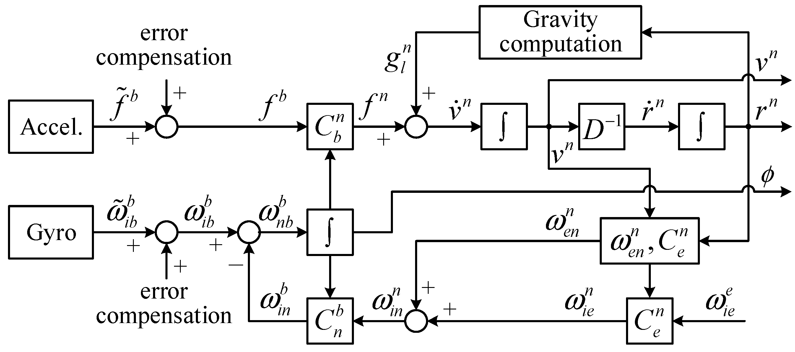
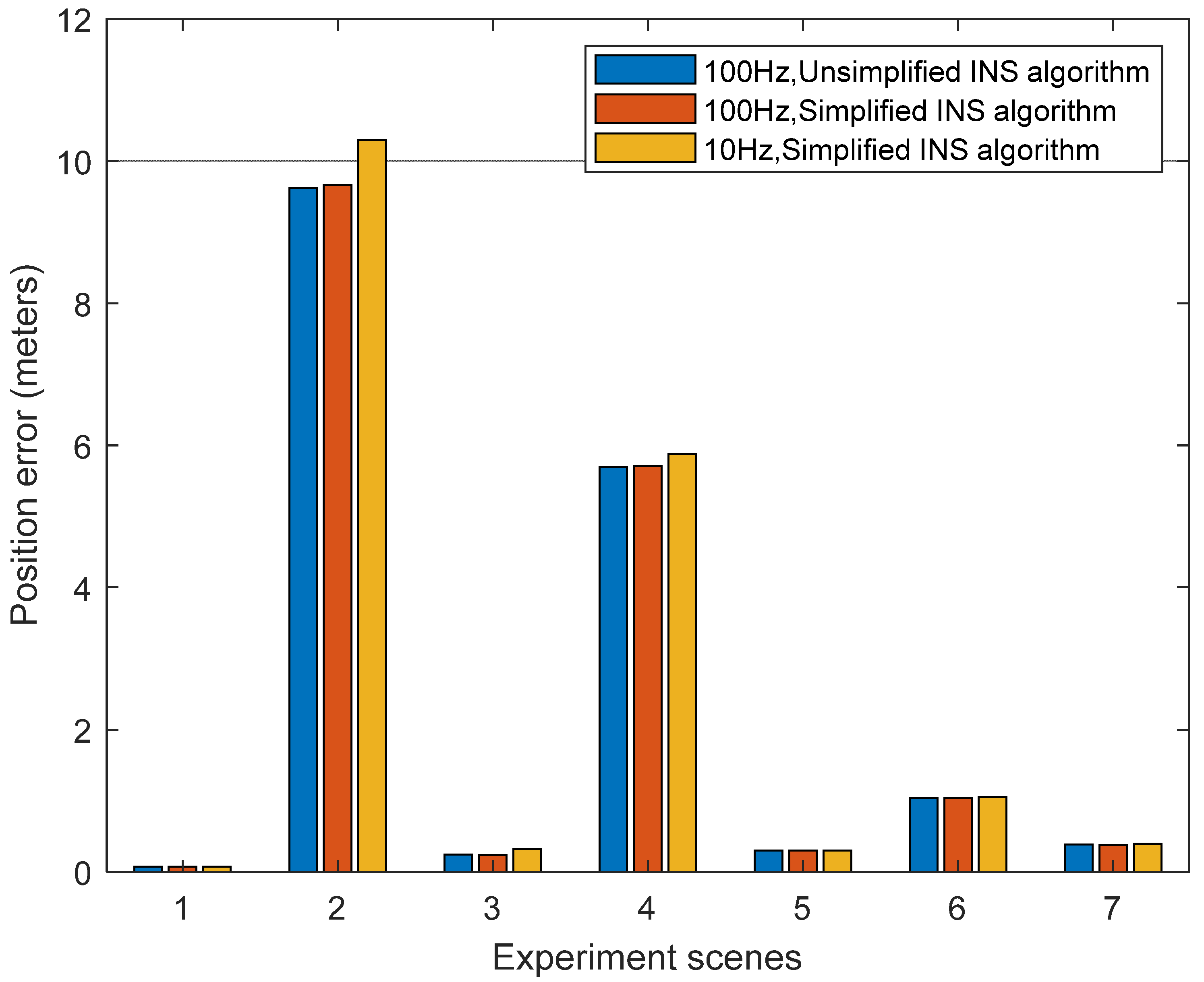
31]. To reduce the system’s power consumption without significantly decreasing the positioning accuracy, a combination of unsimplified and simplified algorithms are used in the MEMS-INS algorithm. When the GNSS signal does not have a fixed solution, the 100 Hz INS mechanization update rate and an unsimplified MEMS-INS algorithm are used to slow down the inertial navigation divergence. When the GNSS signal has a fixed solution, the 10 Hz INS mechanization update rate and a simplified INS algorithm reduce the system’s power consumption.
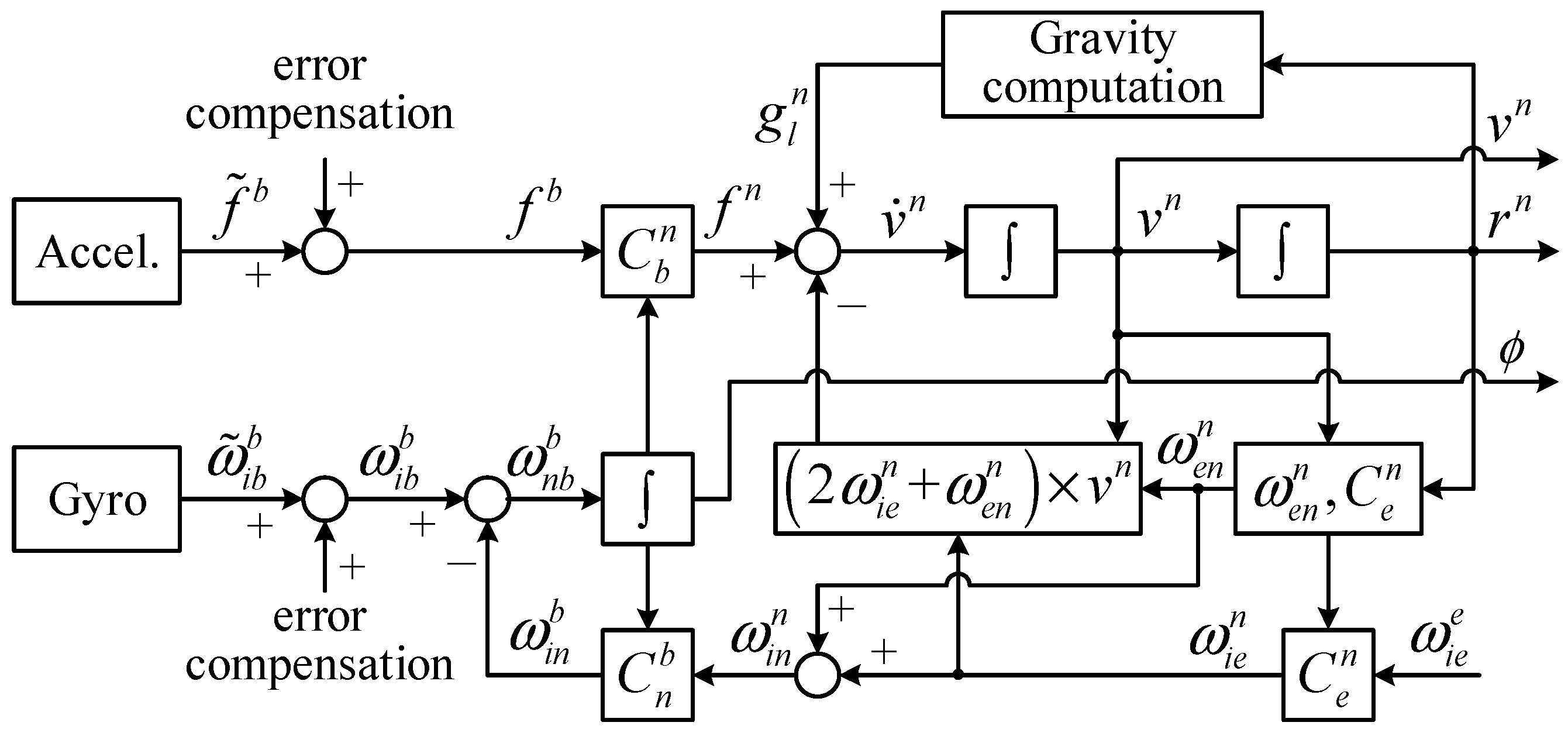
The unsimplified INS algorithm block diagram is shown in Figure 2, and the dynamic equation may be expressed as [22,32].
v ˙ n = C b n f b ( 2 ω i e n + ω e n n ) × v n + g l n
C ˙ n e = C n e ( ω e n n × )
h ˙ = v D
C ˙ b n = C b n ( ω i b b × ) ( ω i n n × ) C b n
where C b n is the rotation matrix from the body frame (b-frame, Forward-Right-Down) to the navigation frame (n-frame, North-East-Down); f b is the specific force in the b-frame; ω i e n is the angular rate of the earth frame (e-frame) relative to the inertial frame (i-frame) in the n-frame; ω e n n is the angular rate of the n-frame relative to the e-frame in the n-frame; v n is the velocity in the n-frame; g l n is the normal gravity in the local position in the n-frame; C n e is the rotation matrix from the n-frame to the e-frame, which represent the geodetic latitude and longitude; h and v D are the ellipsoid height and velocity in the down direction, respectively; ω i b b is the angular rate of the b-frame relative to the i-frame in the b-frame; ω i n n is the angular rate of the n-frame relative to the i-frame in the n-frame; ( × ) is skew symmetric matrix.
According to Equation (3), the unsimplified INS speed update can be written as follows:
v k n = v k 1 n + Δ v f , k n + Δ v g / c o r , k n
where Δ v g / c o r , k n is the velocity increment due to the gravity and Coriolis force and Δ v f , k n is the velocity increment due to the specific force, which can be written as follows [33]:
Δ v g / c o r , k n = [ g l , k 1 / 2 n ( 2 ω i e , k 1 / 2 n + ω e n , k 1 / 2 n ) × v k 1 / 2 n ] Δ t k
Δ v f , k n = [ I [ 0.5 ( ω i e , k 1 / 2 n + ω e n , k 1 / 2 n ) Δ t k × ] ] C b ( k 1 ) n ( k 1 ) Δ v f , k b ( k 1 )
Δ v f , k b ( k 1 ) Δ v f , k b + 1 2 Δ θ k × Δ v f , k b + 1 12 ( Δ θ k 1 × Δ v f , k b + Δ v f , k 1 b × Δ θ k )
where I is a 3-dimensional identity matrix. Equation (10), 1 2 Δ θ k × Δ v f , k b represents the rotational compensation term and 1 12 ( Δ θ k 1 × Δ v f , k b + Δ v f , k 1 b × Δ θ k ) defines sculling compensation term, Δ θ k is the angular increment at a time t k .
The rotation quaternion from the n-frame to the e-frame contains latitude and longitude information. Thus, the position update is solved by quaternion multiplication.
q n ( k ) e ( k ) = q e ( k 1 ) e ( k ) q n ( k 1 ) e ( k 1 ) q n ( k ) n ( k 1 )
where q n ( k ) n ( k 1 ) and q e ( k 1 ) e ( k ) are the quaternion for the n-frame and e-frame, respectively. The asterisk in the formula represents the multiplication symbol.
The rotation vector is used for attitude update, and the attitude quaternion update algorithm can be described as
q b ( k ) n ( k ) = q n ( k 1 ) n ( k ) q b ( k 1 ) n ( k 1 ) q b ( k ) b ( k 1 )
where q b ( k ) b ( k 1 ) is the quaternion for the b-frame.
In MEMS inertial sensors, gyro bias and acceleration bias are the primary sources of errors, which affect the positioning accuracy. To reduce the computational load and thus the power consumption, the MEMS-INS mechanization algorithm is simplified. The error sources that have little influence on the positioning are ignored, such as coriolis acceleration, rotation correction, rotation sculling correction, and coning correction. The simplified INS algorithm block diagram is shown in Figure 3. The dynamic equation is defined as
v ˙ n = C b n f b + g l n
r ˙ n = D 1 v n
q ˙ b n = 0.5 W q b n
where f b is the specific force in the b-frame, g l n is the normal gravity in the local position in the n-frame, D 1 is the transition matrix, and W is the carrier attitude angular rate. D 1 and W can be written as follows:
D 1 = [ 1 R M + h 0 0 0 1 ( R N + h ) cos φ 0 0 0 1 ]
W = [ 0 ω n b , x b ω n b , y b ω n b , z b ω n b , x b 0 ω n b , z b ω n b , y b ω n b , y b ω n b , z b 0 ω n b , x b ω n b , z b ω n b , y b ω n b , x b 0 ]
where R M and R N represent the radius of curvature in the meridian and the prime vertical radius of curvature, respectively; φ is latitude; and ω n b b = ω i b b C n b ( ω i e n + ω e n n ) is the angular rate of the b-frame relative to the n-frame in the b-frame.
Formula (15) is the differential equation of Formula (28). For simplification purposes, angular rate can be assumed as a constant in a short sampling interval Δ t ; that is, a one-sample algorithm of rotation vector is applied. Since the quaternion algorithm is actually a one-sample algorithm, we can obtain the analytic discrete solution of attitude quaternion given by Formula (15).
q b n ( t k + 1 ) = exp { 1 2 t k t k + 1 W d t } q b n ( t k )
S = t k t k + 1 W d t = t k t k + 1 [ 0 ω n b , x b ω n b , y b ω n b , z b ω n b , x b 0 ω n b , z b ω n b , y b ω n b , y b ω n b , z b 0 ω n b , x b ω n b , z b ω n b , y b ω n b , x b 0 ] d t = [ 0 Δ θ x Δ θ y Δ θ z Δ θ x 0 Δ θ z Δ θ y Δ θ y Δ θ z 0 Δ θ x Δ θ z Δ θ y Δ θ x 0 ]
exp { 1 2 t k t k + 1 W d t } = e S 2 = I 4 cos Δ θ 2 + S Δ θ sin Δ θ 2
where I 4 is a 4-dimensional identity matrix. Substitute Formula (20) into Formula (18),
q b n ( t k ) = ( I 4 cos Δ θ 2 + S Δ θ sin Δ θ 2 ) q b n ( t k 1 )
Sort out the above formula as follows:
q b n ( t k ) = q b n ( t k 1 ) + [ ( cos θ 2 1 ) I 4 + 1 θ sin θ 2 S ] q b n ( t k 1 )
where θ = | Δ θ | ; S = W Δ t . Introduce variables
c = 2 ( cos θ 2 1 ) = θ 2 4 + θ 4 192 +
s = 2 θ sin θ 2 = 1 θ 2 24 + θ 4 1920 +
Here, taking c = θ 2 4 , s = 1 , substitute them into (22) to obtain the simplified attitude update equation,
q k = q k 1 + 0.5 ( θ 2 4 I 4 + S ) q k 1
Considering the impact caused by the second and third terms on the right-hand side of Equation (10), navigation accuracy may be minimal. Meanwhile, the quaternion algorithm is a one-sample algorithm, which can be used to obtain the analytic discrete solution of attitude quaternion given in Equation (15). Therefore, the simplified INS update algorithm is given by
v k n = v k 1 n + C b ( k 1 ) n ( k 1 ) Δ v f , k b + g l n Δ t k
r k n = r k 1 n + D 1 ( v k n + v k 1 n ) 2 Δ t k
q k = q k 1 + 0.5 ( θ 2 4 I 4 + S ) q k 1
where Δ θ = Δ θ i b b C n b ( ω i e n + ω e n n ) Δ t is the compensated angular increment.

2.2.2. Simplification of Kalman Filter and Model

In a standard Kalman filter, the prediction state covariance matrix (P matrix) calculation time accounts for about 70% of the Kalman filtering process [30]. To decrease the computation load, a simplified Kalman filter algorithm in the integrated navigation is proposed. This section introduces the simplified Kalman filter algorithm model, error state model, GNSS measurement model, odometer measurement model, and NHC measurement model.
  • Simplification Kalman filter model
In traditional integrated navigation Kalman filters, P matrix prediction and error state updates are performed together, significantly increasing the computation load, which is not suitable for systems with real-time and low power consumption requirements. In our research, the Kalman filter algorithm is improved, and the P matrix prediction is performed together with the measurement update, which dramatically reduces the computation load. The improved algorithm is as follows:
Prediction:
x k , k 1 = Φ k , k 1 x k
Update:
P k , k 1 = Φ k , k 1 P k Φ k , k 1 T + Q k 1
K k = P k , k 1 H k T ( H k P k , k 1 H k T + R k ) 1
x k = x k , k 1 + K k ( z k H k x k , k 1 )
P k = ( I K k H k ) P k , k 1 ( I K k H k ) T + K k R k K k T
where x is the error state vector, which can be omitted since it is reset to zero after each feedback and has no predictable meaning; Φ represents the state transition matrix; P is the error state covariance matrix; Q is the system noise covariance matrix; K is the Kalman filter gain matrix which determines the weights of measurement information when error state is updated; H represents the design matrix; R stands for the covariance matrix of measurement noise; z represents the measurement vector. All the subscripts indicate the state change. For example, x k , k 1 means the error state vector from epoch k 1 to epoch k .
The state transition matrix Φ can be written as follows:
Φ = [ I 3 + ( ω e n n × ) Δ t I 3 0 0 0 F 21 I 3 + [ ( 2 ω i e n ω e n n ) × ] Δ t ( f n × ) Δ t 0 C b n Δ t 0 0 I 3 + ( ω i n n × ) Δ t C b n Δ t 0 0 0 0 1 / t g b 0 0 0 0 0 1 / t a b ]
where F 21 = [ g l n R M R N + h Δ t 0 0 0 g l n R M R N + h Δ t 0 0 0 2 g l n R M R N + h Δ t ] , I 3 is a 3-dimensional identity matrix, f n is the specific force in the n-frame; t g b is the gyro zero-bias correlation time, t a b is the accelerometer zero bias correlation time.
In Equation (30), the update accuracy of the P matrix mainly depends on the state transition matrix Φ . Taking the P matrix prediction of three adjacent epochs k , k + 1 and k + 2 in the traditional Kalman filter as an example to derive the update of the P matrix in the improved Kalman filter, the process is as follows:
Epoch k :
Q k = 1 2 ( Φ k + 1 , k Q ¯ k + Q ¯ k Φ k + 1 , k T ) Δ t
P k + 1 , k = Φ k + 1 , k P k Φ k + 1 , k T + Q k
Epoch k + 1 :
Q k + 1 = 1 2 ( Φ k + 2 , k + 1 Q ¯ k + 1 + Q ¯ k + 1 Φ k + 2 , k + 1 T ) Δ t
P k + 2 , k + 1 = Φ k + 2 , k + 1 P k + 1 Φ k + 2 , k + 1 T + Q k + 1 = ( Φ k + 2 , k + 1 Φ k + 1 , k ) P k ( Φ k + 2 , k + 1 Φ k + 1 , k ) T +   Q k + 1 + Φ k + 2 , k + 1 Q k Φ k + 2 , k + 1 T
Epoch k + 2 :
Q k + 2 = 1 2 ( Φ k + 3 , k + 2 Q ¯ k + 2 + Q ¯ k + 2 Φ k + 3 , k + 2 T ) Δ t
P k + 3 , k + 2 = Φ k + 3 , k + 2 P k + 2 Φ k + 3 , k + 2 T + Q k + 2 = ( Φ k + 3 , k + 2 Φ k + 2 , k + 1 Φ k + 1 , k ) P k ( Φ k + 3 , k + 2 Φ k + 2 , k + 1 Φ k + 1 , k ) T +   Q k + 2 + Φ k + 3 , k + 2 Q k + 1 Φ k + 3 , k + 2 T + ( Φ k + 3 , k + 2 Φ k + 2 , k + 1 ) Q k ( Φ k + 3 , k + 2 Φ k + 2 , k + 1 ) T
where Q is the constant spectral density matrix; Q ¯ k Q ¯ k + 1 Q ¯ k + 2 is the system noise covariance matrix, Δ t is the sampling interval of the navigation system.
Compared with (36), (38), and (40), it is found that the structures of the three formulas are similar, and the matrix plays a crucial role in each epoch of the P matrix. The second term on the right side of Equation (40) is the current constant spectral density matrix, which is easy to calculate. It is mainly because the latter two terms on the right side of the equal sign are challenging to handle. Therefore, these two terms are expanded and named s 1 and s 2 as follows:
s 1 = Φ k + 3 , k + 2 Q k + 1 Φ k + 3 , k + 2 T = 1 2 [ ( Φ k + 3 , k + 2 Φ k + 2 , k + 1 ) ( Q ¯ k + 1 Φ k + 3 , k + 2 T ) + ( Φ k + 3 , k + 2 Q ¯ k + 1 ) ( Φ k + 3 , k + 2 Φ k + 2 , k + 1 ) T ] Δ t
s 2 = ( Φ k + 3 , k + 2 Φ k + 2 , k + 1 ) Q k ( Φ k + 3 , k + 2 Φ k + 2 , k + 1 ) T = 1 2 [ ( Φ k + 3 , k + 2 Φ k + 2 , k + 1 Φ k + 1 , k ) Q ¯ k ( Φ k + 3 , k + 2 Φ k + 2 , k + 1 ) T +   ( Φ k + 3 , k + 2 Φ k + 2 , k + 1 ) Q ¯ k ( Φ k + 3 , k + 2 Φ k + 2 , k + 1 Φ k + 1 , k ) T ] Δ t
Since the first term of (40) is to multiply the state transition matrix of each epoch, the calculation form is simple, and the operations amount is small. Therefore, for ease of calculation, the last two terms in (40) are constructed into the form of the first term, that is, s 1 and s 2 are approximate, as shown in s 3 and s 4 below:
s 3 = 1 2 [ ( Φ k + 3 , k + 2 Φ k + 2 , k + 1 Φ k + 1 , k ) Q ¯ k + 1 + Q ¯ k + 1 ( Φ k + 3 , k + 2 Φ k + 2 , k + 1 Φ k + 1 , k ) T ] Δ t
s 4 = 1 2 [ ( Φ k + 3 , k + 2 Φ k + 2 , k + 1 Φ k + 1 , k ) Q ¯ k + 1 + Q ¯ k + 1 ( Φ k + 3 , k + 2 Φ k + 2 , k + 1 Φ k + 1 , k ) T ] Δ t
Since Δ t is very small, the state transition matrix in the above formula can be written as follows:
Φ k + 3 , k + 2 I + F 3 Δ t
Φ k + 2 , k + 1 I + F 2 Δ t
Φ k + 1 , k I + F 1 Δ t
Substitute (45), (46), (47) into s 3 s 1 and s 4 s 2 to perform high-order small quantity analysis, as shown below:
s 4 s 2 = 1 2 [ ( Φ k + 3 , k + 2 Φ k + 2 , k + 1 Φ k + 1 , k ) Q ¯ k + 1 + Q ¯ k + 1 ( Φ k + 3 , k + 2 Φ k + 2 , k + 1 Φ k + 1 , k ) T ] Δ t   1 2 [ ( Φ k + 3 , k + 2 Φ k + 2 , k + 1 Φ k + 1 , k ) Q ¯ k ( Φ k + 3 , k + 2 Φ k + 2 , k + 1 ) T + ( Φ k + 3 , k + 2 Φ k + 2 , k + 1 ) Q ¯ k ( Φ k + 3 , k + 2 Φ k + 2 , k + 1 Φ k + 1 , k ) T ] Δ t = 1 2 ( Δ t 2 + F 1 Δ t 3 + F 2 Δ t 3 + F 3 Δ t 3 + F 2 F 1 Δ t 4 + F 3 F 1 Δ t 4 + F 3 F 2 Δ t 4 + F 3 F 2 F 1 Δ t 5 ) Q ¯ k ( F 2 + F 3 + F 3 F 2 Δ t ) T   1 2 ( F 2 + F 3 + F 3 F 2 Δ t ) Q ¯ k ( Δ t 2 + F 1 Δ t 3 + F 2 Δ t 3 + F 3 Δ t 3 + F 2 F 1 Δ t 4 + F 3 F 1 Δ t 4 + F 3 F 2 Δ t 4 + F 3 F 2 F 1 Δ t 5 ) T
s 3 s 1 = 1 2 [ ( Φ k + 3 , k + 2 Φ k + 2 , k + 1 Φ k + 1 , k ) Q ¯ k + 1 + Q ¯ k + 1 ( Φ k + 3 , k + 2 Φ k + 2 , k + 1 Φ k + 1 , k ) T ] Δ t   1 2 [ ( Φ k + 3 , k + 2 Φ k + 2 , k + 1 ) ( Q ¯ k + 1 Φ k + 3 , k + 2 T ) + ( Φ k + 3 , k + 2 Q ¯ k + 1 ) ( Φ k + 3 , k + 2 Φ k + 2 , k + 1 ) T ] Δ t = 1 2 ( Δ t 2 + F 2 Δ t 3 + F 3 Δ t 3 + F 2 F 3 Δ t 4 ) F 1 Q ¯ 1 2 ( Δ t 2 + F 2 Δ t 3 + F 3 Δ t 3 + F 2 F 3 Δ t 4 ) F 3 T Q ¯   + 1 2 Q ¯ F 1 T ( Δ t 2 + F 2 Δ t 3 + F 3 Δ t 3 + F 2 F 3 Δ t 4 ) T 1 2 Q ¯ F 3 ( Δ t 2 + F 2 Δ t 3 + F 3 Δ t 3 + F 2 F 3 Δ t 4 ) T
Observation (48) and (49) shows that all terms in the two equations are high order small quantities of Δ t . Thus, two equations can be approximated as a zero matrix within an acceptable range. Therefore, the P matrix prediction from k epochs to k + 2 epochs can be described as
P k + 3 , k = ( Φ k + 3 , k + 2 Φ k + 2 , k + 1 Φ k + 1 , k ) P k ( Φ k + 3 , k + 2 Φ k + 2 , k + 1 Φ k + 1 , k ) T   + 1 2 ( Φ k + 3 , k + 2 Q ¯ k + 2 + Q ¯ k + 2 Φ k + 3 , k + 2 T ) Δ t   + 2 1 2 [ ( Φ k + 3 , k + 2 Φ k + 2 , k + 1 Φ k + 1 , k ) Q ¯ k + 1 + Q ¯ k + 1 ( Φ k + 3 , k + 2 Φ k + 2 , k + 1 Φ k + 1 , k ) T ] Δ t
Similarly, the P matrix prediction is extended to n epochs, namely from k epochs to k + n epochs, as follows:
P k + n , k = Φ k + n , k P k Φ k + n , k T + 1 2 ( Φ k + n , k + n 1 Q ¯ k + n 1 + Q ¯ k + n 1 Φ k + n , k + n 1 T ) Δ t   + 1 2 ( Φ k + n , k Q ¯ k + n 1 + Q ¯ k + n 1 Φ k + n , k T ) ( n 1 ) Δ t
where
Φ k + n , k = Φ k + n , k + n 1 Φ k + n 1 , k + n 2 Φ k + 2 , k + 1 Φ k + 1 , k
  • Error State Model
To improve the navigation accuracy of low-cost MEMS inertial sensors while reducing the computation tasks, the bias error of the gyroscope and accelerometer and the scale factor of the odometer are augmented into the filter state and estimated online [34]. Therefore, the error state vector of Kalman filtering can be written as:
δ x = [ ( δ r n ) T ( δ v n ) T ϕ T b g T b a T s o d o T ] T
where δ r n = [ δ r N δ r E δ r D ] T and δ v n = [ δ v N δ v E δ v D ] T are the position and velocity errors in the n-frame, respectively; ϕ = [ ϕ r o l l ϕ p i t c h ϕ h e a d i n g ] T is the attitude error; b g is the gyro bias; b a is the accelerometer bias; s o d o denotes the odometer scale factor. The first five and the last terms of Equation (53) correspond to a three-dimensional vector and one-dimensional vector, respectively.
  • GNSS Measurement Model
The position of the phase center of the GNSS antenna is calculated from the INS navigation results and the measured value of the lever arm as follows [35]:
r G N S S n = r I M U n + D R 1 C b n l G N S S b
where r I M U n is the position of the IMU measurement center, and l G N S S b is the lever arm from the IMU measurement center to the GNSS antenna phase center resolved in the b-frame.
For loosely coupled integration, the measurement vector is expressed as the difference between the position estimated by INS and the position solved by GNSS, and the lever arm effect from the INS center to the GNSS antenna is considered. Hence, the measurement equation based on GNSS position can be expressed as
z r G N S S = C e n ( r ^ G N S S e r ˜ G N S S e ) = C e n ( r ^ I M U e r ˜ G N S S e ) + C b n l G N S S b
where C e n is the rotation matrix from the earth frame (e-frame) to the n-frame; r ^ G N S S e and r ˜ G N S S e are the estimated position of the GNSS antenna phase center and the measurement position of the GNSS receiver in the e-frame, respectively; r ^ I M U e is the estimated position of the IMU measurement center in the e-frame.
  • Odometer Measurement Model
The relationship between the vehicle velocity and the IMU velocity can be established by the lever arm, which represents the spatial position relationship between the vehicle and the IMU measurement center, and can be expressed as [36]
v ^ o d o v = C b v C n b v I M U n + C b v ( ω n b b × ) l o d o b
where C b v is the rotation matrix from b-frame to the vehicle frame (v-frame); C n b stands for the rotation matrix from the n-frame to the b-frame; v I M U n is the velocity of the IMU measurement center; l o d o b is the lever arm from the IMU measurement center to the odometer center, which is resolved in the body frame. The estimated velocity at the odometer center is shown as v ^ o d o v = [ v ^ o d o , x v v ^ o d o , y v v ^ o d o , z v ] T .
The odometer output velocity measurement is as follows
v ˜ o d o , y v = v y v
where v ˜ o d o , y v is the one-dimensional velocity measurement in the v-frame and v y v is the speed output from the odometer. However, the actual velocity measurement can be expressed as [37]
v ˜ o d o , y v = v y v e y v
where e y v is the odometer velocity measurement noise, which is modeled as Gaussian white noise. Thus, the velocity error measurement equation in the v-frame can be expressed as
z v o d o = v ^ o d o , y v v ˜ y v = ( C b v C n b δ v I M U n C b v C n b ( v I M U n × ) ϕ C b v ( l o d o b × ) δ ω i b b ) y + e y v
where v ^ o d o , y v is the forward estimated velocity at the odometer center.
  • NHC Measurement Model
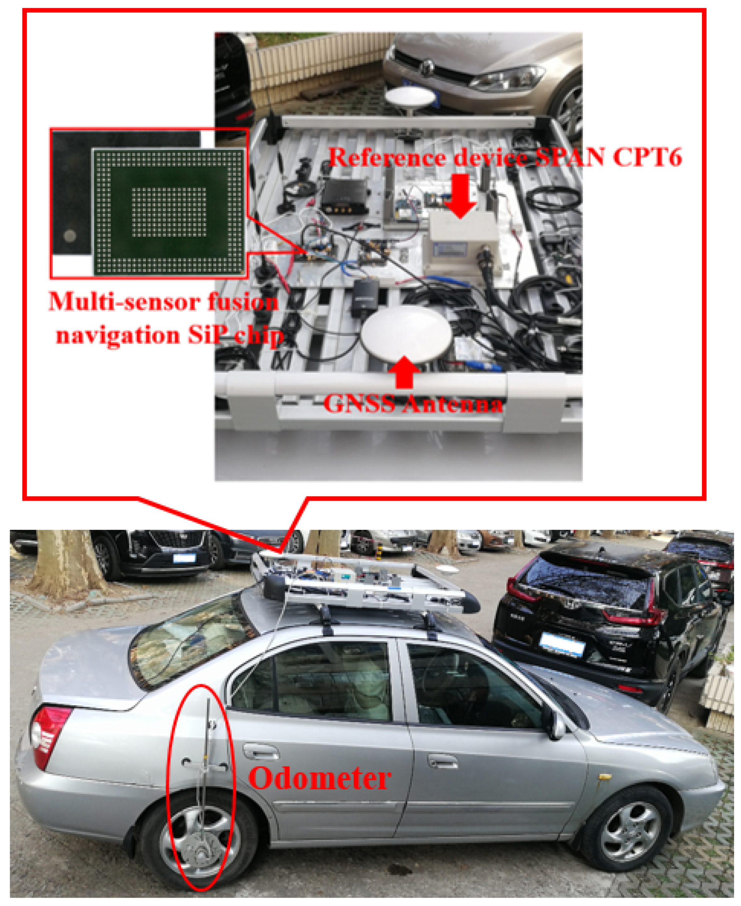
For land vehicle applications, vehicles carrying a GNSS/MEMS-IMU integrated navigation system can maintain reliable and continuous rigid contact with the road while driving on the road. Thus, the motion of the land vehicle on the road is governed by two non-holonomic constraints because the vehicle does not jump off the road or slide on the road. Therefore, the lateral and vertical velocity of the vehicle are zero, and the measurement in the vehicle frame can be expressed as [38,39,40,41,42]
v ˜ x v 0 v ˜ z v 0
where v ˜ x v and v ˜ z v represent the velocity components of the vehicle in the plane perpendicular to the forward direction (y-axis).
The NHC velocity error measurement equation in the vehicle frame can be expressed as
z v o d o = [ v ^ o d o , x v v ˜ x v v ^ o d o , z v v ˜ z v ] = ( C b v C n b δ v I M U n C b v C n b ( v I M U n × ) ϕ C b v ( l o d o b × ) δ ω i b b ) x , z + [ e x v e z v ]
where v ^ o d o , x v and v ^ o d o , z v are the lateral and vertical estimated velocity at the odometer center, respectively; e x v and e z v are the lateral and vertical velocity measurements noise, respectively; the symbol ( ) x , z represents the first and third rows of the three-dimensional vector.
When the vehicle is stationary, the odometer-derived speed v y v is zero, and in this case, a zero-velocity update can be used to update the INS solution [43,44].

3. Analysis of Computation Load

In order to evaluate the efficiency of the algorithm, the operands (1 s period) of addition (A), subtraction (S), multiplication (M), division (D), square roots (SR), and trigonometrics (T) of the INS mechanization and Kalman filter in the integrated navigation algorithm are investigated. Table 1, Table 2, Table 3 and Table 4, respectively, count the number of operations in INS mechanization and the Kalman filter in the process of ZUPT, GNSS measurement update, odometer measurement update, and NHC measurement update.
Table 1 shows the operands required for different INS mechanizations at different data rates. From this table, it is clear that the modified algorithm has a better computational efficiency compared to the standard one, and the number of operations can be reduced by about 72.5% at a 100 Hz data rate. On the other hand, the computation load is also affected by the data rate. The number of operations can be reduced by about 97.3% at a 10 Hz data rate.
Table 2 shows the operands required by the standard and simplified Kalman filter algorithm in the ZUPT process. In the standard algorithm, Kalman prediction and update are 100 Hz and 1 Hz, respectively. However, in the simplified algorithm, the Kalman prediction and update are both 1 Hz. It can be seen from the table that the simplified algorithm has a more significant impact on the number of operations, which can be reduced by about 96.5%.
Table 3 shows the number of operations required for different Kalman filter algorithms in the GNSS measurement update process. Similar to Table 2, the simplified algorithm (prediction and update are both 1 Hz) significantly impacts the computation load, which can be reduced by about 80.8%.
Table 4 shows the number of operations required by different Kalman filter algorithms during odometer and NHC measurement updating. Similarly, after improving the algorithm, the computation load can be reduced by nearly 77.3%.
In summary, the INS mechanization and Kalman filter algorithm modification can reduce the number of operations. In addition, the data rate has a significant impact on the computation load [45]. Therefore, combining the simplified algorithm with reducing the sampling rate can significantly improve computational efficiency.

4. Experimental Scene Introduction and Hardware Platform Description

To evaluate the dynamic adaptive power adjustment strategy and positioning accuracy of single-frequency GNSS/MEMS-IMU/odometer simplified integrated navigation algorithms in complex scenes. The real-time performance verification experiment is carried out in complex scenes, including boulevard, tunnel, overhead bridge, and urban street. The trajectory is shown in Figure 4, and the natural environment of six complex scenes in Figure 4 is shown in Figure 5. It includes boulevard 1, tunnel 1, boulevard 2, tunnel 2, overhead bridge, and urban street. Boulevard 1 has dense trees on both sides and narrow roads. Tunnel 1 and tunnel 2 are V-shaped tunnels which go downhill first and then uphill, and there are turning sections inside the tunnels. Boulevard 2 is near the mountain. On the right side of the road is the hillside. At the same time, there are dense trees on both sides of the road. The overhead bridge scene is that the overhead bridge almost blocks the sky on the left side of the road, and the receiver can track only the GNSS signal on the right side of the sky. City streets are scenes with buildings and street trees on both sides of the road. In these scenes, the satellite signal is easy to be blocked, or there is multipath interference, which affects the positioning accuracy of the receiver.
The vehicle-mounted hardware experimental platform and reference equipment used in this research are shown in Figure 6. The SiP packaging process integrates multiple sensors into one chip to form a multi-sensor fusion navigation SiP chip (including MEMS IMU, a magnetometer, single-frequency GNSS, MCU, NB-IoT, e-sim, and barometer, temperature, and humidity sensors). At the same time, the navigation level equipment NovAtel SPAN CPT-6 (dual-frequency GNSS RTK/fiber IMU tightly coupled system) is taken as a reference to evaluate the positioning accuracy of SiP chip. Table 5 shows the performance specifications of the different levels of IMUs in the two devices. The IMU data rate of the two devices is 100 Hz, and the real-time navigation result output frequency is 1 Hz and 100 Hz, respectively. In addition, vehicle speed information is introduced to improve the SiP chip’s positioning accuracy when the GNSS signal is blocked. The odometer is installed on the vehicle’s right rear wheel to measure the vehicle’s speed, and this information is provided to the SiP chip for assisting MEMS IMU navigation.
In the real-time vehicle navigation experiment, to measure the power consumption of SiP chips, a high-precision power meter is used to record and store the chip’s power consumption in real-time but does not include NB-IoT and e-sim.

5. Results

5.1. Simplified INS Algorithms Performance Verification

The position drift of the system after GNSS outages is the most critical indicator to measure the accuracy of INS. To verify the performance of the INS, the INS will work completely independently without the assistance of other external sensors, such as GNSS and odometers. The trajectory of the inertial navigation performance verification experiment is shown in Figure 7. The blue markers in the figure in this trajectory select six sections and simulate GNSS interruption for 60 s in each section. The road section includes bumps, turns, up and down slopes, acceleration, and deceleration.
The RMS statistical results of the position drift error of the unsimplified INS algorithm with a 100 Hz data rate, simplified INS algorithm with a 100 Hz data rate, and simplified INS algorithm with a 10 Hz data rate within 60 s of GNSS outages are shown in Figure 8. The position error of the unsimplified INS algorithm with a 100 Hz data rate are used as reference. The main difference between simplified and unsimplified algorithms is that it omits Coriolis acceleration, rotation correction, sculling correction, and coning correction. It can be seen from the figure that the error of ➁ and ➂ are relatively large. The main reason is that ➁ is a turning scene. According to the reference [21], the prominent position drift error in this section is mainly caused by the omission of the rotation correction. On the other hand, ➂ is primarily due to the higher speed and turning. Therefore, the position drift error in this section is mainly caused by the omission of Coriolis acceleration and rotation correction [21].
Compare the positioning results of INS with NovAtel SPAN CPT-6 to obtain the positioning error, and perform quantitative analysis, as shown in Table 6. The degradation in Table 6 represents the degradation percentage of the positioning error of the simplified algorithm relative to the positioning error of the unsimplified algorithm. Compared with the unsimplified algorithm with a data rate of 100 Hz, the simplified algorithm has an error of less than 2% in the other four scenarios except for scenarios ➁ and ➂. It can also be seen from the table that reducing the data rate has a more significant impact on the performance of the inertial navigation system.

5.2. Complex Scene Simplified Algorithm Verification

The GNSS receiver has high positioning accuracy in open scenarios, and it is not suitable to evaluate the simplified algorithm. Therefore, the route in Figure 4 is selected to verify the performance of the simplified algorithm (simplified Kalman filter and simplified INS mechanization). It is mainly divided into zero velocity state scenarios, non-zero velocity state scenarios with RTK fixed/float solution, and non-zero velocity state scenarios without RTK fixed/float solution.

5.2.1. Simplified Kalman Filter Algorithm

  • Zero velocity state scenarios
In this research, a reliable high-resolution pulse encoder is used as an odometer in the integrated navigation system. The encoder can generate 4096 pulses per circle. The TIM_encoder peripheral of MCU detects the number of pulses and calculates the vehicle speed. The TIM_encoder peripheral has a filtering function to filter out some pulse interference signals. The integrated navigation system determines whether to execute ZUPT by detecting the vehicle’s speed, and the speed threshold is 0.1 m/s. This value can prevent system misjudgment caused by interference signals. When the vehicle velocity is zero, the integrated navigation system performs a 10 Hz data rate simplified INS mechanization and adopts the simplified Kalman filter algorithm with one-step P matrix prediction. The results of the simplified and unsimplified algorithms are compared with NovAtel SPAN CPT-6, and the positioning error of the unsimplified Kalman filter algorithm and unsimplified INS mechanization algorithm with 100 Hz data rate are used as a reference. In Figure 9a, the position and velocity errors of the unsimplified Kalman filter algorithm are shown in the red circle. The position error remains unchanged, while the velocity error converges to near zero. Figure 9b shows the position and velocity errors of the simplified Kalman filter algorithm. The result is the same as Figure 9a. The position error remains unchanged, and the speed error converges to zero. Comparing them in Table 7 shows that the simplified Kalman filter algorithm and the unsimplified Kalman filter algorithm have little effect on the position error after ZUPT.
  • Non-zero velocity state scenarios with RTK fixed/float solution
Boulevard 1, boulevard 2, overhead bridge, and urban street in Figure 4 are selected to verify the performance of the simplified Kalman filter algorithm in non-zero velocity state scenarios with RTK fixed/float solution. In these scenarios, if the GNSS is a fixed solution, the system only performs the simplified INS mechanization algorithm with 10 Hz data rate and simplified Kalman filter algorithm. However, if it is a float solution, the INS data rate becomes 100 Hz, and the odometer information and NHC information are combined to assist INS. In this case, the results of the unsimplified and simplified algorithms are compared with NovAtel SPAN CPT-6, and the positioning error of the unsimplified Kalman filter algorithm with a 100 Hz IMU data rate is used as a reference. Figure 10 shows the position errors comparison between the unsimplified Kalman filter algorithm and the simplified Kalman filter algorithm. It can be seen from Table 8 that the simplified algorithm can roughly maintain the same positioning accuracy as the unsimplified Kalman filter algorithm in the non-zero speed state with RTK fixed/float solution.
  • Non-zero velocity state without RTK fixed/float solution
Tunnel 1 and tunnel 2 in Figure 4 are selected as the test scenarios to verify the performance of the simplified Kalman filter algorithm in non-zero velocity state without RTK fixed/float solution. In these two scenarios, there is no GNSS signal, only the speed information output by the odometer and the lateral and longitudinal constraints of the vehicle, that is, NHC information to assist INS. The update rate of the speed and NHC is 10 Hz, and the IMU data rate is 100 Hz. In this case, the results of the unsimplified and simplified algorithms are compared with NovAtel SPAN CPT-6, and the positioning error of the unsimplified Kalman filter algorithm with a 100 Hz IMU data rate is used as a reference. Figure 11 shows a comparison of the position error between the unsimplified and simplified Kalman filter algorithm. It can be seen from the figure that the simplified algorithm has little effect on the positioning accuracy compared with the unsimplified Kalman filter algorithm. According to Table 9, the position error of the simplified algorithm in tunnel 1 degrades by 3.2% relative to the unsimplified algorithm, and in tunnel 2 it degrades by 7.4%. However, this degradation is within an acceptable range.

5.2.2. Simplified INS Mechanization

The zero-velocity state scenario, boulevard 1, tunnel 1, boulevard 2, tunnel 2, overhead bridge, and urban street in Figure 4 are selected as the test scenarios to verify the performance of the simplified INS mechanization algorithm. GNSS signal is interrupted in these test sections, and only the odometer and NHC assisted the INS. Under this condition, the simplified INS mechanization and unsimplified INS mechanization algorithm are quantitatively analyzed. The positioning error obtained by comparing the positioning results of the simplified and unsimplified algorithms with NovAtel SPAN CPT-6 is shown in Figure 12. It can be seen from the figure that the positioning error of the 100 Hz data rate simplified algorithm is almost the same as that of the 100 Hz data rate unsimplified algorithm, indicating that the simplified INS algorithm has little effect on the positioning accuracy in complex scenarios. However, compared with the positioning error of the simplified algorithm with a data rate of 10 HZ and the unsimplified algorithm with a data rate of 100 Hz, the positioning accuracy of the former deteriorates more severely on some road sections. According to Table 10, compared with the unsimplified algorithm with a 100 Hz data rate, the maximum deterioration of the simplified INS algorithm with a 100 Hz data rate is only 0.21%. It is even slightly better than the unsimplified algorithm on some road sections. Due to the reduced sampling rate, the simplified algorithm with a 10 Hz data rate in tunnel 1 is 34.7% worse than the unsimplified algorithm with a 100 Hz data rate, but this is within an acceptable range. In the seven scenarios, the GPS interruption time is different, the longest is 150 s, and the shortest is only 15 s, while the maximum positioning error is 10.295 m, and the minimum is 0.07 m. However, the positioning error is not related to time, mainly caused by factors such as the vehicle speed, system state, and road environment.

5.3. Complex Scene Positioning Performance Verification

GNSS signals are susceptible to environmental interference, resulting in decreased positioning accuracy, especially single-frequency GNSS [46,47]. The horizontal positioning error of GNSS in the experimental route is shown in Figure 13. In the figure, the GNSS solution status is marked with green, yellow, and red on the x-axis. Green indicates that the current GNSS status is a fixed solution, and the positioning error can reach about 2 cm. Yellow means that the GNSS status is a float solution, and the positioning error is less than 1 m. However, serious errors occasionally occur, and the maximum value has reached 6 m. Red indicates the differential solution mainly caused by the GNSS signal being blocked in tunnel 1 and tunnel 2. It can be seen from the figure that most of the position results in the whole experimental route are float solutions. The GNSS positioning error is the largest at the two tunnels. As shown in the enlarged part of the figure, the maximum value exceeds 110 m.
The six complex scenarios in Figure 4 are selected to verify the real-time positioning performance of the simplified algorithm (including the simplified INS mechanization algorithm and simplified Kalman filter algorithm). The RMS statistical horizontal position error of six scenes (boulevard 1, tunnel 1, boulevard 2, tunnel 2, overhead bridge, and urban street) are shown in Figure 14. The positioning error of the unsimplified algorithm is blue, and the simplified algorithm is red. In this case, the results of the simplified and unsimplified algorithms (including the 100 Hz data rate unsimplified INS mechanization algorithm and unsimplified Kalman filtering algorithm and integrating odometer information and NHC information) are compared with NovAtel SPAN CPT-6, and the positioning error of the unsimplified algorithm is used as a reference. It can be seen from Figure 14 that there is little difference in the position error between the unsimplified and simplified algorithms. The positioning errors of the six scenes in the figure are analyzed quantitatively, as shown in Table 11. The degradation of the RMS statistical position error of the six scenes is less than 0.1%. Even in some scenarios, the value of the simplified algorithm is better than the value of the unsimplified algorithm, which is theoretically reasonable.
The simplified integrated navigation algorithm in the whole road section controls the data rate and selects the observation information to update the measurement according to different scenes and motion modes. The real-time position error is shown in Figure 15. At the same time, it also shows the position error of the unsimplified integrated navigation algorithm in the whole experimental route. It can be seen from the figure that the north and east direction position errors of the simplified algorithm have little degradation compared to the unsimplified algorithm. However, in the down direction, the simplified algorithm has a large fluctuation in the early stage. The main reason is that GNSS is a fixed solution during this period, and the IMU data rate is only 10 Hz, and there is no external sensor assistance. Generally speaking, in the process of vehicle navigation, vertical error is rarely concerned. Therefore, compared with the unsimplified algorithm, the horizontal positioning error obtained by the simplified algorithm has an acceptable degree of degradation.
For vehicle navigation, velocity is another crucial parameter. Therefore, in a complex environment, it is necessary to analyze the speed accuracy of the simplified integrated navigation algorithm. The real-time velocity error of the single-frequency GNSS RTK/MEMS-IMU/odometer integrated navigation with simplified and unsimplified algorithms in the whole experimental route is shown in Figure 16. The error curves in the north and east directions are similar, and the maximum values are less than 0.25 m/s. However, the error of the simplified algorithm in the early stage of the down direction fluctuates wildly, but it tends to be consistent after the later convergence. It can be seen from the figure that no matter whether the algorithm is unsimplified or simplified, the errors in the north and east directions are relatively small, and the trends of the two are basically the same.
Similar to position and velocity, attitude accuracy is also necessary for vehicle navigation applications. Figure 17 shows the attitude error curve of the integrated navigation system in the experiment route. The roll, pitch, and yaw errors of the simplified algorithm in the first 200 s are quite different from those of the unsimplified algorithm. The slower convergence speed of INS mainly causes this during this period. Since the IMU used in the research is MEMS grade, yaw angle is more susceptible to drift than roll angle and pitch angles. In other words, the yaw angle error increases faster than the roll and pitch, which can also be observed in Figure 17. However, the more significant influence on the positioning error in the integrated navigation algorithm is the yaw rather than the roll and pitch. It can be seen from the figure that the simplified algorithm has a significant fluctuation in the yaw error in the first 100 s and then stabilizes and is less than 2 degrees.
The real-time position, velocity, and attitude RMS and STD statistics of the entire experimental route are shown in Table 12. According to the statistical results of north and east position errors, the horizontal position RMS and STD of the unsimplified integrated navigation algorithm are 0.339 m and 0.289 m, respectively. In comparison, the simplified algorithm is 0.336 m and 0.287 m, respectively. Therefore, the horizontal position error of the simplified algorithm is slightly better than that of the unsimplified algorithm, which is reasonable in theory. For the unsimplified and simplified algorithms, the north, east, and down direction velocities RMS and STD are less than 0.055 m/s. However, the simplified algorithm degrades 71.8% and 65.6% in terms of down direction velocity compared with the unsimplified algorithm. The main reason for this error is that the ground-up position error is large, and there is no speed observation information in the vertical direction. In terms of attitude error, the roll RMS and STD of the simplified algorithm are smaller than those of the unsimplified algorithm, while the pitch and heading are degraded. Compared with the unsimplified algorithm, the pitch RMS and STD of the simplified algorithm are devalued by 8.52% and 7.03%, respectively, but this degradation is within an acceptable range.

5.4. Complex Scene Real-Time Power Consumption Verification

The performance of the simplified algorithm in the multi-sensor fusion navigation SiP is evaluated. The algorithm can meet the requirements of sub-meter high-precision positioning and low power consumption. The vehicle power meter and power supply are used to measure the power consumption of SiP chips in real-time and high-precision navigation in complex scenes, and the power consumption data in the process is saved. The result of power consumption data plotting is shown in Figure 18, and its average value is 141 mW.
In a word, compared with the unsimplified algorithm, the position, speed, and attitude degradation of the simplified algorithm are relatively small, and the algorithm running on the SiP chip consumes less power, which meets the requirements of low power consumption without sacrificing the positioning accuracy.

6. Discussion

Positioning accuracy and power consumption in a complex urban environment are two opposing indicators. The trade-off between these two indicators is an urgent matter for integrated navigation chips. According to the presented results, the single-frequency GNSS/MEMS-IMU/odometer integrated navigation simplified algorithm with adaptive power consumption adjustment can meet the requirements of positioning accuracy and power consumption at the same time in complex scenarios. It can be seen from Table 1 that the simplified INS algorithm omits small items that have little effect on the positioning accuracy, so that the calculation amount is reduced by about 72.5% compared with the unsimplified algorithm. However, if a combination of the simplified algorithm and down-sampling is applied, the computation load can be reduced by about 97.3%, and the degradation of positioning error is within an acceptable range. Furthermore, the one-step prediction method used in the simplified Kalman filter algorithm dramatically reduces the computation of the Kalman filter. It can be seen from Figure 9, Figure 10 and Figure 11 that in different scenarios, using different observation information for measurement update, the simplified algorithm has little impact on the positioning accuracy compared with the unsimplified algorithm.
The real-time test results of single-frequency GNSS/MEMS-IMU/odometer simplified integrated navigation algorithm with adaptive power consumption adjustment in complex scenes are shown in Figure 15, Figure 16 and Figure 17. It can be seen from the figure that the position, velocity, and attitude error curves of the simplified and unsimplified algorithms are highly similar, except for the time when the system converges at the initial moment. The main reason for the longer convergence time is that the IMU data rate is 10 Hz and only GNSS observation information is available. The real-time power consumption after the simplified algorithm is shown in Figure 18. The average power consumption in the entire test section is 141 mW, including GNSS, MEMS-IMU, magnetometers, barometers, temperature and humidity sensors, and MCU.

7. Conclusions

This paper proposes a single-frequency GNSS/MEMS-IMU/odometer real-time high-precision simplified integrated navigation algorithm with dynamic power adaptive adjustment capability in complex environments. It is implemented in a multi-sensor fusion navigation SiP chip. The simplified INS algorithm and the simplified Kalman filter algorithm are combined with the strategy of adaptively adjusting the data rate and selecting the observation information for measurement update in different scenarios and sports modes to achieve high-precision positioning and low power consumption in complex scenarios.
In this paper, the simplified INS algorithm and the simplified Kalman filter algorithm are analyzed theoretically, and the computational complexity of the algorithm is counted. At the same time, the real-time verification of complex scenes is carried out. According to the statistical results, the simplified algorithm dramatically reduces the computation load compared with the unsimplified algorithm. Furthermore, the experimental results show that the positioning accuracy of the simplified algorithm degrades very little compared with the unsimplified algorithm.
In summary, the proposed simplified algorithm will not cause a decrease in navigation accuracy while reducing power consumption. In other words, the algorithm simplification does not sacrifice accuracy. The test results of a single-frequency GNSS/MEMS-IMU/odometer simplified integrated navigation algorithm with adaptive dynamic power adjustment in complex scenes are shown in Table 12. The results show that it is feasible to apply the proposed simplified integrated navigation algorithm to vehicle navigation. It is of great significance for applications that require demanding a real-time response.

Author Contributions

Conceptualization, J.J., J.L. (Jingnan Liu) and P.Y.; methodology, J.J. and P.Y.; software, P.Y.; validation, J.J. and P.Y.; formal analysis, J.J., P.Y. and F.Z.; investigation, J.J. and P.Y.; resources, J.J. and P.Y.; writing—original draft preparation, J.J. and P.Y.; writing—review and editing, J.J., P.Y., D.X., Y.T., J.W. and J.L. (Jianghua Liu); visualization, D.X.; supervision, J.J. and P.Y.; project administration, Y.T.; funding acquisition, J.J. All authors have read and agreed to the published version of the manuscript.

Funding

This research was funded by the National Key Research and Development Program of China (2018YFB0505200 and 2018YFB0505201), the Fundamental Research Funds for the Central Universities (2042018kf0253), the Guiding project of scientific research plan of Hubei Ministry of Education (B2019154), and the PhD research foundation of Hubei University of Science and Technology (BK201801).

Institutional Review Board Statement

Not applicable.

Informed Consent Statement

Not applicable.

Data Availability Statement

Not applicable.

Acknowledgments

Thank you very much for the equipment support of Jinguang Jiang’s research group, for his driving experiment for this research, and for the technical support of Fangning Zhang, Dongpeng Xie, Yanan Tang, Jiaji Wu and Chao Zhang.

Conflicts of Interest

The authors declare no conflict of interest.

References

  1. Niu, X.; Nasser, S.; Goodall, C.; El-Sheimy, N. A Universal Approach for Processing any MEMS Inertial Sensor Configuration for Land-Vehicle Navigation. J. Navig. 2007, 60, 233–245. [Google Scholar] [CrossRef]
  2. Kaplan, E.D.; Hegarty, C. Understanding GPS Principles and Applications; Artech House Publishers: Boston, MA, USA; London, UK, 2005; pp. 214–215. [Google Scholar]
  3. Savage, P.G. Strapdown Analytics: Part 1 and 2; Strapdown Associates, Inc.: Maple Plain, MN, USA, 2000; pp. 214–215. [Google Scholar]
  4. Titterton, D.; Weston, J. Strapdown Inertial Navigation Technology; Institution of Engineering and Technology: London, UK, 2004; pp. 214–215. [Google Scholar]
  5. Jekeli, C. Inertial Navigation Systems with Geodetic Applications; Walter de Gruyter: Berlin, Germany, 2012; pp. 214–215. [Google Scholar]
  6. Stepanov, O.A. Optimal and Suboptimal Filtering in Integrated Navigation Systems. Aerosp. Navig. Syst. 2016, 244–298. [Google Scholar] [CrossRef]
  7. Al Bitar, N.; Gavrilov, A.I. Comparative Analysis of Fusion Algorithms in a Loosely-Coupled Integrated Navigation System on the Basis of Real Data Processing. Gyroscopy Navig. 2019, 10, 231–244. [Google Scholar] [CrossRef]
  8. Niu, X.; Nassar, S.; El-Sheimy, N. An Accurate Land-Vehicle MEMS IMU/GPS Navigation System Using 3D Auxiliary Velocity Updates. Navigation 2007, 54, 177–188. [Google Scholar] [CrossRef]
  9. Bruder, S.; El-Osery, A. Low-Cost Inertial Navigation. In Control and Systems Engineering; El-Osery, A., Prevost, J., Eds.; Springer: Cham, Switzerland, 2015; Volume 27, pp. 231–259. [Google Scholar]
  10. Odolinski, R.; Teunissen, P. Low-cost, high-precision, single-frequency GPS–BDS RTK positioning. GPS Solut. 2017, 21, 1315–1330. [Google Scholar] [CrossRef]
  11. Wendel, J.; Meister, O.; Schlaile, C.; Trommer, G.F. An integrated GPS/MEMS-IMU navigation system for an autonomous helicopter. Aerosp. Sci. Technol. 2006, 10, 527–533. [Google Scholar] [CrossRef]
  12. Sasani, S.; Asgari, J.; Amiri-Simkooei, A. Improving MEMS-IMU/GPS integrated systems for land vehicle navigation applications. GPS Solut. 2015, 20, 89–100. [Google Scholar] [CrossRef]
  13. Li, T.; Zhang, H.; Gao, Z.; Chen, Q.; Niu, X. High-Accuracy Positioning in Urban Environments Using Single-Frequency Multi-GNSS RTK/MEMS-IMU Integration. Remote Sens. 2018, 10, 205. [Google Scholar] [CrossRef] [Green Version]
  14. Li, T.; Zhang, H.; Gao, Z.; Niu, X.; El-Sheimy, N. Tight Fusion of a Monocular Camera, MEMS-IMU, and Single-Frequency Multi-GNSS RTK for Precise Navigation in GNSS-Challenged Environments. Remote Sens. 2019, 11, 610. [Google Scholar] [CrossRef] [Green Version]
  15. Zharkov, M.V.; Veremeenko, K.K.; Antonov, D.; Kuznetsov, I. Attitude Determination Using Ambiguous GNSS Phase Measurements and Absolute Angular Rate Measurements. Gyroscopy Navig. 2018, 9, 277–286. [Google Scholar] [CrossRef]
  16. Schwarz, K.P.; Naser, E.-S. Mobile Mapping Systems-State of the Art and Future Trends. ISPRS. Arch. 2004, 35, 10. [Google Scholar]
  17. Supej, M. 3D measurements of alpine skiing with an inertial sensor motion capture suit and GNSS RTK system. J. Sports Sci. 2010, 28, 759–769. [Google Scholar] [CrossRef]
  18. Fasel, B.; Spörri, J.; Gilgien, M.; Boffi, G.; Chardonnens, J.; Müller, E.; Aminian, K. Three-Dimensional Body and Centre of Mass Kinematics in Alpine Ski Racing Using Differential GNSS and Inertial Sensors. Remote Sens. 2016, 8, 671. [Google Scholar] [CrossRef] [Green Version]
  19. Godha, S.; Lachapelle, G.; Cannon, E. Integrated GPS/INS System for Pedestrian Navigation in a Signal Degraded Environment. In Proceedings of the 19th International Technical Meetings of the Satellite Division of the Institute of Navigation, Fort Worth, TX, USA, 26–29 September 2006. [Google Scholar]
  20. Rehman, A.; Shahid, H.; Afzal, M.A.; Bhatti, H.M.A. Accurate and Direct GNSS/PDR Integration Using Extended Kalman Filter for Pedestrian Smartphone Navigation. Gyroscopy Navig. 2020, 11, 124–137. [Google Scholar] [CrossRef]
  21. Zhang, Q.; Niu, X.; Zhang, H.; Shi, C. Algorithm Improvement of the Low-End GNSS/INS Systems for Land Vehicles Navigation. Math. Probl. Eng. 2013, 2013, 1–12. [Google Scholar] [CrossRef]
  22. Shin, E.-H. Accuracy Improvement of Low Cost INS/GPS for Land Applications. Master's Thesis, The University of Calgary, Calgary, AB, Canada, 2001. [Google Scholar]
  23. Jordan, J. An Accurate Strapdown Direction Cosine Algorithm; National Aeronautics and Space Administration: Washington, DC, USA, 1969. [Google Scholar]
  24. Bortz, J.E. A New Mathematical Formulation for Strapdown Inertial Navigation. IEEE Trans. Aerosp. Electron. Syst. 1971, 7, 61–66. [Google Scholar] [CrossRef]
  25. Wu, Y.; Cai, Q.; Truong, T.-K. Fast RodFIter for Attitude Reconstruction from Inertial Measurements. IEEE Trans. Aerosp. Electron. Syst. 2018, 55, 419–428. [Google Scholar] [CrossRef] [Green Version]
  26. Ushaq, M.; Fang, J.C. An Improved and Efficient Algorithm for SINS/GPS/Doppler Integrated Navigation Systems. Appl. Mech. Mater. 2012, 245, 323–329. [Google Scholar] [CrossRef]
  27. Emami, M.; Taban, M.R. A Low Complexity Integrated Navigation System for Underwater Vehicles. J. Navig. 2018, 71, 1161–1177. [Google Scholar] [CrossRef]
  28. Zhu, Q.J.; Yan, G.M.; Yang, P.X.; Qin, Y.Y. A Rapid Computation Method for Kalman Filtering in Vehicular SINS/GPS Integrated System. Appl. Mech. Mater. 2012, 182–183, 541–545. [Google Scholar] [CrossRef]
  29. Hu, S.; Xu, S.; Wang, D.; Zhang, A. Optimization Algorithm for Kalman Filter Exploiting the Numerical Characteristics of SINS/GPS Integrated Navigation Systems. Sensors 2015, 15, 28402–28420. [Google Scholar] [CrossRef]
  30. Li, Q.; Ban, Y.; Niu, X.; Zhang, Q.; Gong, L.; Liu, J. Efficiency Improvement of Kalman Filter for GNSS/INS through One-Step Prediction of P Matrix. Math. Probl. Eng. 2015, 2015, 1–13. [Google Scholar] [CrossRef]
  31. Kraft, M. Micromachined Inertial Sensors: The State-of-the-Art and a Look into the Future. Meas. Control. 2000, 33, 164–168. [Google Scholar] [CrossRef] [Green Version]
  32. Shin, E.H. Estimation Techniques for Low-Cost Inertial Navigation. Ph.D. Thesis, The University of Calgary, Calgary, AB, Canada, 2005. [Google Scholar]
  33. Niu, X.; Zhang, Q.; Gong, L.; Liu, C.; Zhang, H.; Shi, C.; Wang, J.; Coleman, M. Development and evaluation of GNSS/INS data processing software for position and orientation systems. Surv. Rev. 2014, 47, 87–98. [Google Scholar] [CrossRef]
  34. Niu, X.; Wu, J.; Zhang, Q. Research on Measurement Error Model of GNSS/INS Integration Based on Consistency Analysis. Gyroscopy Navig. 2018, 9, 243–254. [Google Scholar] [CrossRef]
  35. Zhang, Q.; Chen, Q.; Niu, X.; Shi, C. Requirement Assessment of the Relative Spatial Accuracy of a Motion-Constrained GNSS/INS in Shortwave Track Irregularity Measurement. Sensors 2019, 19, 5296. [Google Scholar] [CrossRef] [Green Version]
  36. Chen, Q.; Zhang, Q.; Niu, X.; Wang, Y. Positioning Accuracy of a Pipeline Surveying System Based on MEMS IMU and Odometer: Case Study. IEEE Access 2019, 7, 104453–104461. [Google Scholar] [CrossRef]
  37. Zhou, Y.; Chen, Q.; Niu, X. Kinematic Measurement of the Railway Track Centerline Position by GNSS/INS/Odometer Integration. IEEE Access 2019, 7, 157241–157253. [Google Scholar] [CrossRef]
  38. Zhang, Q.; Hu, Y.; Niu, X. Required Lever Arm Accuracy of Non-Holonomic Constraint for Land Vehicle Navigation. IEEE Trans. Veh. Technol. 2020, 69, 8305–8316. [Google Scholar] [CrossRef]
  39. Chen, Q.; Niu, X.; Zuo, L.; Zhang, T.; Xiao, F.; Liu, Y.; Liu, J. A Railway Track Geometry Measuring Trolley System Based on Aided INS. Sensors 2018, 18, 538. [Google Scholar] [CrossRef] [Green Version]
  40. Dissanayake, G.; Sukkarieh, S.; Nebot, E.; Durrant-Whyte, H. The aiding of a low-cost strapdown inertial measurement unit using vehicle model constraints for land vehicle applications. IEEE Trans. Robot. Autom. 2001, 17, 731–747. [Google Scholar] [CrossRef] [Green Version]
  41. Chen, Q.; Niu, X.; Zhang, Q.; Cheng, Y. Railway Track Irregularity Measuring by GNSS/INS Integration. Navigation 2015, 62, 83–93. [Google Scholar] [CrossRef]
  42. Syed, Z.F.; Aggarwal, P.; Niu, X.; El-Sheimy, N. Civilian Vehicle Navigation: Required Alignment of the Inertial Sensors for Acceptable Navigation Accuracies. IEEE Trans. Veh. Technol. 2008, 57, 3402–3412. [Google Scholar] [CrossRef]
  43. Jiang, Q.; Wu, W.; Li, Y.; Jiang, M. Millimeter Scale Track Irregularity Surveying Based on ZUPT-Aided INS with Sub-Decimeter Scale Landmarks. Sensors 2017, 17, 2083. [Google Scholar] [CrossRef] [Green Version]
  44. Cai, Q.; Yang, G.; Song, N.; Pan, J.; Liu, Y. An Online Smoothing Method Based on Reverse Navigation for ZUPT-Aided INSs. J. Navig. 2016, 70, 342–358. [Google Scholar] [CrossRef]
  45. Lee, J.K.; Choi, M.J. Effect of Strapdown Integration Order and Sampling Rate on IMU-Based Attitude Estimation Accuracy. Sensors 2018, 18, 2775. [Google Scholar] [CrossRef] [Green Version]
  46. Robustelli, U.; Baiocchi, V.; Pugliano, G. Assessment of Dual Frequency GNSS Observations from a Xiaomi Mi 8 Android Smartphone and Positioning Performance Analysis. Electronics 2019, 8, 91. [Google Scholar] [CrossRef] [Green Version]
  47. Guo, L.; Wang, F.; Sang, J.; Lin, X.; Gong, X.; Zhang, W. Characteristics Analysis of Raw Multi-GNSS Measurement from Xiaomi Mi 8 and Positioning Performance Improvement with L5/E5 Frequency in an Urban Environment. Remote Sens. 2020, 12, 744. [Google Scholar] [CrossRef] [Green Version]
Figure 1. The algorithm flow chart of single-frequency GNSS/MEMS-IMU/odometer real-time, high-precision, and low-power simplified integrated navigation. The strategy of adaptive adjustment of data rate and selection of observation information for measurement update in different scenes and motion modes is adopted.
Remotesensing 13 03236 g001
Figure 2. The block diagram of the unsimplified INS algorithm.
Remotesensing 13 03236 g002
Figure 3. The block diagram of the simplified INS algorithm.
Remotesensing 13 03236 g003
Figure 4. Real-time performance verification experiment trajectory of vehicle navigation in complex scenarios.
Remotesensing 13 03236 g004
Figure 5. The natural environment of six complex scenarios.
Remotesensing 13 03236 g005
Figure 6. Vehicle experimental platform and equipment.
Remotesensing 13 03236 g006
Figure 7. ➀–➅ MEMS INS performance verification experiment trajectory, in which six blue marked sections are simulated GNSS interrupt for 60 s.
Remotesensing 13 03236 g007
Figure 8. Position drift error in 60 s GPS outages with different INS algorithms and different data rates.
Remotesensing 13 03236 g008
Figure 9. Horizontal error and velocity error of ZUPT in different Kalman filter algorithms: (a) unsimplified Kalman filter algorithm with 100 Hz IMU data rates; (b) simplified Kalman filter algorithm with 10 Hz IMU data rates.
Remotesensing 13 03236 g009
Figure 10. Position errors of the unsimplified and simplified Kalman filter algorithm in boulevard 1, boulevard 2, overhead bridge, and urban street.
Remotesensing 13 03236 g010
Figure 11. Position errors of the unsimplified and simplified Kalman filter algorithm in Tunnel 1 and Tunnel 2.
Remotesensing 13 03236 g011
Figure 12. Position drift error of the different INS algorithms and different data rates in the scenarios of zero velocity state, boulevard 1, tunnel 1, boulevard 2, tunnel 2, overhead bridge, and urban street.
Remotesensing 13 03236 g012
Figure 13. GNSS horizontal position error in the experimental route.
Remotesensing 13 03236 g013
Figure 14. Position errors of the unsimplified algorithm and the proposed simplified algorithm in the complex scene.
Remotesensing 13 03236 g014
Figure 15. The real-time position errors of unsimplified and simplified integrated navigation algorithms in the north, east, and down directions in the experimental route.
Remotesensing 13 03236 g015
Figure 16. The real-time velocity errors of unsimplified and simplified integrated navigation algorithms in the north, east, and down directions in the whole experimental route.
Remotesensing 13 03236 g016
Figure 17. The real-time attitude errors of unsimplified and simplified integrated navigation algorithms in the whole experimental route.
Remotesensing 13 03236 g017
Figure 18. The real-time power consumption of the proposed simplified integrated navigation algorithms in the whole experimental route.
Remotesensing 13 03236 g018
Table 1. Operand number (in 1 s cycle) and improved efficiency between standard and simplified INS algorithms.
MA&SDSRT
Standard algorithm (100 Hz)36,60032,00054007002200
Modified algorithm (100 Hz)10,400 (71.5%)8800 (72.5%)2800 (48.2%)400 (42.9%)1400 (36.4%)
Modified algorithm (10 Hz)1040 (97.2%)880 (97.3%)280 (94.8%)40 (94.3%)140 (93.7%)
Table 2. Operand number (in 1 s cycle) and improved efficiency between standard and simplified Kalman filtering algorithms in the ZUPT process.
MA&SDSRT
Standard algorithm 241,773224,48923211817
Modified algorithm 9894 (96%)7877 (96.5%)133 (42.6%)118 (0%)17 (0%)
Table 3. Operand number (in 1 s cycle) and improved efficiency between standard and simplified Kalman filtering algorithms in the GNSS measurement update process.
MA&SDSRT
Standard algorithm 215,928203,85123412031
Modified algorithm 52,728 (75.6%)39,151 (80.8%)135 (42.3%)120 (0%)31 (0%)
Table 4. Operand number (in 1 s cycle) and improved efficiency between standard and simplified Kalman filtering algorithms in the odometer and NHC measurement update process.
MA&SDSRT
Standard algorithm 222,353211,03623211817
Modified algorithm 61,777 (72.1%)47,782 (77.3%)133 (42.6%)118 (0%)17 (0%)
Table 5. Performance specifications of the IMU in the experiment.
MEMS GradeNavigation Grade
GyroBias (deg/h)100.027
ARW (deg/sqrt(h))0.270.0667
AccelerometerBias (mGal)180050
VRW (m/s/sqrt(h))0.0420.03
Table 6. Statistic values of position drift error in 60 sec GPS outages.
Scenarios123456
RMS (m)100 Hz, Unsimplified9.56.1717.883.228.39.98
100 Hz, Simplified9.676.5818.623.028.2310.06
Degradation (%)1.76.64.1−6.2−0.80.8
10 Hz, Simplified10.599.0625.453.177.7410.84
Degradation (%)11.546.842.3−1.5−6.78.6
Table 7. Statistic values of the position error of the unsimplified and simplified Kalman filter algorithm in zero velocity scenario.
Scenarios1
RMS (m)Unsimplified0.04
Simplified 0.04
Degradation (%)-
Table 8. Statistic values of the position error of the unsimplified and simplified Kalman filter algorithm in boulevard 1, boulevard 2, overhead bridge, and urban street.
Scenarios1234
RMS (m)Unsimplified 0.190.440.570.33
Simplified 0.2050.440.570.33
Degradation (%)7.8---
Table 9. Statistic values of the position error of unsimplified and simplified Kalman filter algorithm in tunnel 1 and tunnel 2.
Scenarios12
RMS (m)Unsimplified0.620.81
Simplified0.640.87
Degradation (%)3.27.4
Table 10. Statistic values of position drift error of the different INS algorithms and different data rates in the scenarios of zero velocity state, boulevard 1, tunnel 1, boulevard 2, tunnel 2, overhead bridge, and urban street.
Scenarios1234567
GNSS outages duration (s)331502490241560
RMS (m)100 Hz, Unsimplified0.079.6220.2395.6930.2971.0380.383
100 Hz, Simplified0.079.6610.2385.7050.2961.0390.379
Degradation (%)-0.41−0.410.21−0.330.096−1.04
10 Hz, Simplified0.070310.2950.3225.880.2991.0520.393
Degradation (%)0.436.9934.73.280.671.342.61
Table 11. Statistic values of the position error of the unsimplified algorithm and the simplified algorithm.
Scenarios123456
RMS (m)Unsimplified0.160.36350.39060.64290.6490.3256
Simplified0.160.36360.39010.64310.64890.3257
Degradation (%)-0.028−0.130.03−0.0150.03
Table 12. Statistic values of the position, velocity, and attitude errors of the unsimplified and the simplified algorithm in the experimental route.
RMSSTD
PositionNorth (m)Unsimplified0.2600.208
Simplified0.2600.207
Degradation (%)0.00−0.48
East (m)Unsimplified0.2180.201
Simplified0.2140.200
Degradation (%)−1.83−0.49
Down (m)Unsimplified4.3230.998
Simplified4.4731.087
Degradation (%)3.468.91
VelocityNorth (m/s)Unsimplified0.0290.028
Simplified0.0310.030
Degradation (%)6.897.14
East (m/s)Unsimplified0.0350.035
Simplified0.0360.036
Degradation (%)2.852.85
Down (m/s)Unsimplified0.0320.032
Simplified0.0550.053
Degradation (%)71.865.6
AttitudeRoll (deg)Unsimplified0.5670.483
Simplified0.5340.375
Degradation (%)−5.82−22.3
Pitch (deg)Unsimplified0.1290.128
Simplified0.1400.137
Degradation (%)8.527.03
Heading (deg)Unsimplified0.7210.352
Simplified0.7340.361
Degradation (%)1.802.55
Publisher’s Note: MDPI stays neutral with regard to jurisdictional claims in published maps and institutional affiliations.

