
PEMCNet: An Efficient Multi-Scale Point Feature Fusion Network for 3D LiDAR Point Cloud Classification

 , ,
, ,
Abstract
: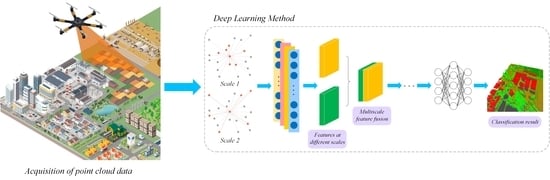
1. Introduction
2. Related Work
2.1. Ball Query Searching Based Feature Learning Networks
2.2. K-NN Searching Based Feature Learning Networks
3. Methodology
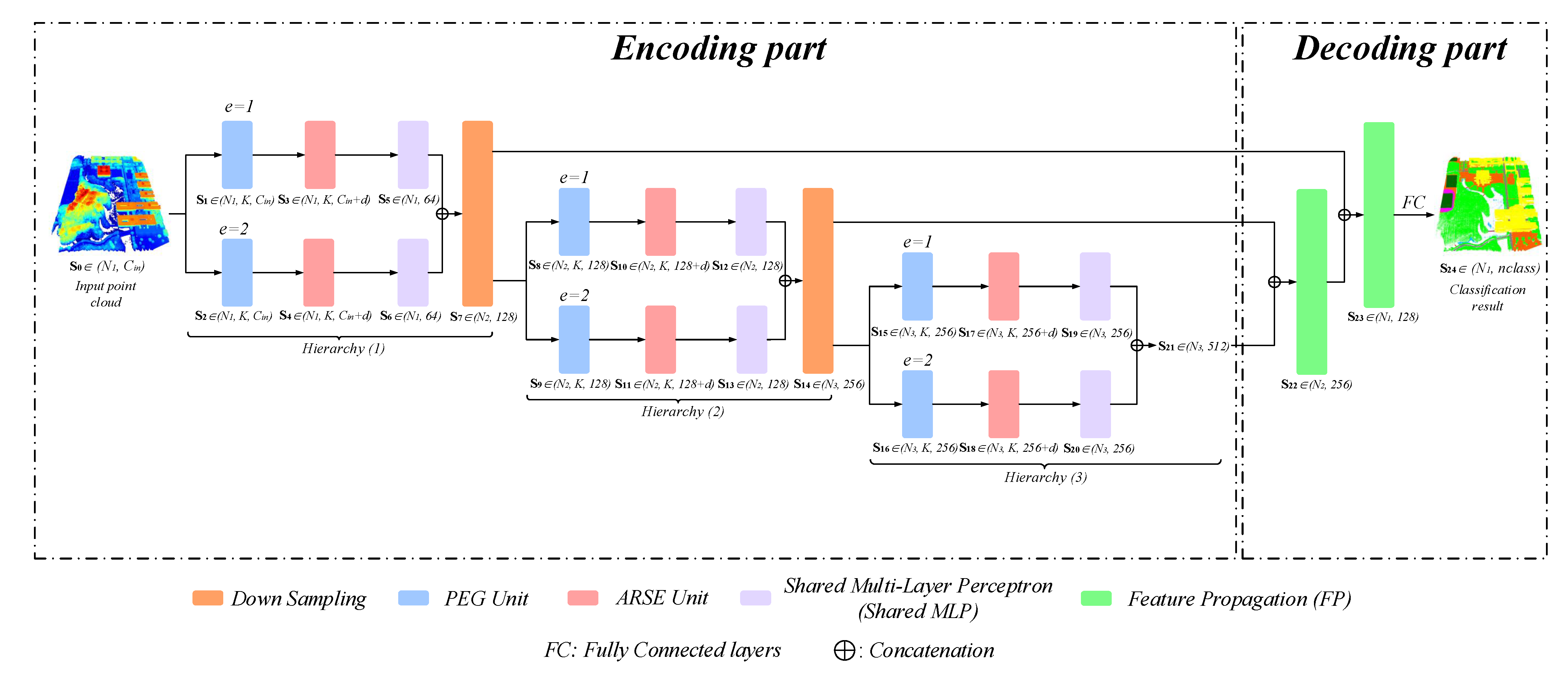
3.1. Network Structure
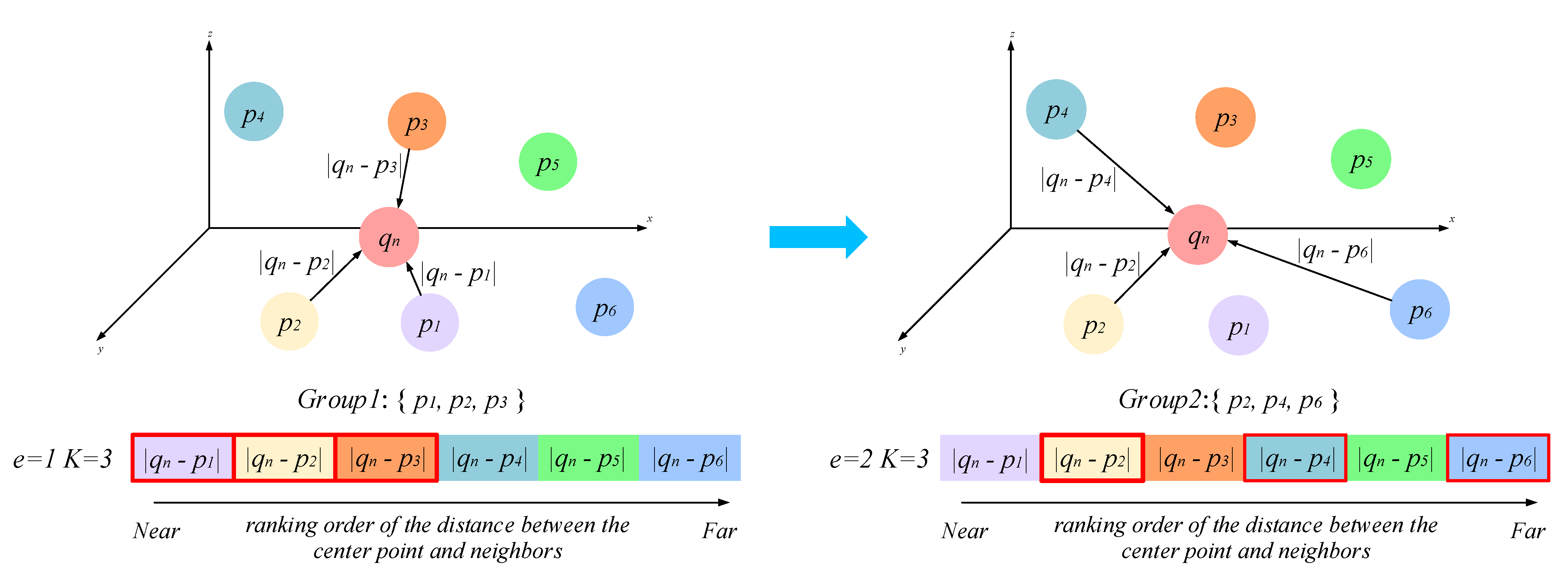
3.2. Feature Learning
3.3. Loss Function
4. Experiment
4.1. Experiments on the Public Datasets
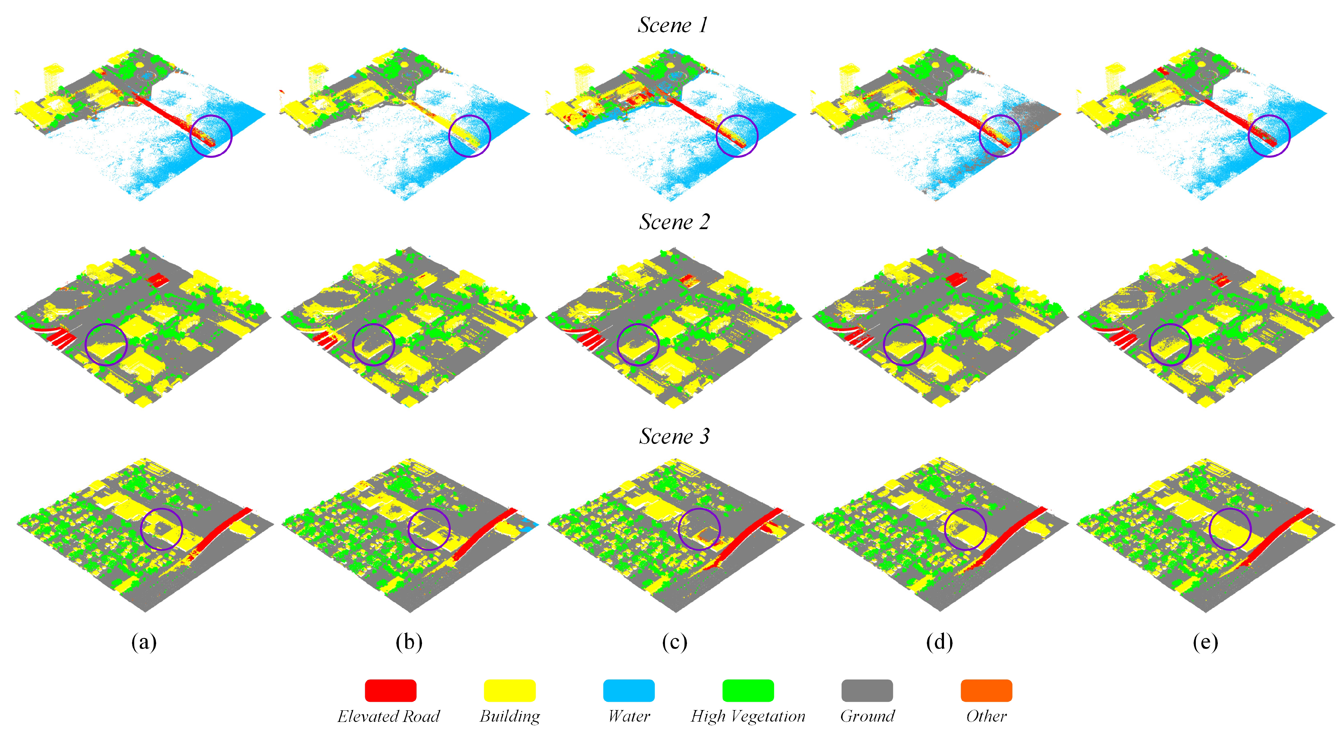
4.2. Classification Results
4.3. Hyperparameter Analysis
4.4. Experiments on the UAV-Based Point Cloud Data
5. Discussion
6. Conclusions
Author Contributions
Funding
Conflicts of Interest
References
- Wen, C.; Yang, L.; Li, X.; Peng, L.; Chi, T. Directionally constrained fully convolutional neural network for airborne LiDAR point cloud classification. ISPRS J. Photogramm. Remote Sens. 2020, 162, 50–62. [Google Scholar] [CrossRef] [Green Version]
- Liu, W.; Sun, J.; Li, W.; Hu, T.; Wang, P. Deep Learning on Point Clouds and Its Application: A Survey. Sensors 2019, 19, 4188. [Google Scholar] [CrossRef] [Green Version]
- Ioannidou, A.; Chatzilari, E.; Nikolopoulos, S.; Kompatsiaris, I. Deep Learning Advances in Computer Vision with 3D Data: A Survey. ACM Comput. Surv. 2017, 50, 20:1–20:38. [Google Scholar] [CrossRef]
- Qiu, Q.; Sun, N.; Bai, H.; Wang, N.; Fan, Z.; Wang, Y.; Meng, Z.; Li, B.; Cong, Y. Field-Based High-Throughput Phenotyping for Maize Plant Using 3D LiDAR Point Cloud Generated with a “Phenomobile”. Front. Plant Sci. 2019, 10, 554. [Google Scholar] [CrossRef] [PubMed] [Green Version]
- Yang, B.; Huang, R.; Li, J.; Tian, M.; Dai, W.; Zhong, R. Automated Reconstruction of Building LoDs from Airborne LiDAR Point Clouds Using an Improved Morphological Scale Space. Remote Sens. 2017, 9, 14. [Google Scholar] [CrossRef] [Green Version]
- Ali, W.; Abdelkarim, S.; Zidan, M.; Zahran, M.; Sallab, A.E. YOLO3D: End-to-End Real-time 3D Oriented Object Bounding Box Detection from LiDAR Point Cloud. In Proceedings of the 2018 European Conference on Computer Vision (ECCV), Munich, Germany, 8–14 September 2018; pp. 1–12. [Google Scholar]
- Neuville, R.; Bates, J.; Jonard, F. Estimating Forest Structure from UAV-Mounted LiDAR Point Cloud Using Machine Learning. Remote Sens. 2021, 13, 352. [Google Scholar] [CrossRef]
- Zhang, W.; Qiu, W.; Song, D.; Xie, B. Automatic Tunnel Steel Arches Extraction Algorithm Based on 3D LiDAR Point Cloud. Sensors 2019, 19, 3972. [Google Scholar] [CrossRef] [PubMed] [Green Version]
- Elbaz, G.; Avraham, T.; Fischer, A. 3D Point Cloud Registration for Localization Using a Deep Neural Network Auto-Encoder. In Proceedings of the IEEE Conference on Computer Vision and Pattern Recognition, Honolulu, HI, USA, 21–26 July 2017; pp. 4631–4640. [Google Scholar]
- Maturana, D.; Scherer, S. 3D Convolutional Neural Networks for landing zone detection from LiDAR. In Proceedings of the IEEE International Conference on Robotics and Automation (ICRA 2015), Seattle, WA, USA, 26–30 May 2015; pp. 3471–3478. [Google Scholar]
- Tonina, D.; McKean, J.A.; Benjankar, R.M.; Wright, C.W.; Goode, J.R.; Chen, Q.; Reeder, W.J.; Carmichael, R.A.; Edmondson, M.R. Mapping river bathymetries: Evaluating topobathymetric LiDAR survey. Earth Surf. Process. Landf. 2019, 44, 507–520. [Google Scholar] [CrossRef]
- Widyaningrum, E.; Gorte, B.G.H. Comprehensive comparison of two image-based point clouds from aerial photos with airborne LiDAR for large-scale mapping. Int. Arch. Photogramm. Remote Sens. Spat. Inf. Sci. 2017, 42, 557–565. [Google Scholar] [CrossRef] [Green Version]
- Chen, S.; Liu, B.; Feng, C.; Vallespi-Gonzalez, C.; Wellington, C. 3D Point Cloud Processing and Learning for Autonomous Driving. arXiv 2020, arXiv:2003.00601. [Google Scholar]
- Wang, M.; Dong, H.; Zhang, W.; Chen, C.; Lu, Y.; Li, H. An End-to-end Auto-driving Method Based on 3D LiDAR. J. Phys. Conf. Ser. 2019, 1288, 012061. [Google Scholar] [CrossRef]
- Chen, X.; Ma, H.; Wan, J.; Li, B.; Xia, T. Multi-view 3D Object Detection Network for Autonomous Driving. In Proceedings of the 2017 IEEE Conference on Computer Vision and Pattern Recognition, CVPR 2017, Honolulu, HI, USA, 21–26 July 2017; pp. 6526–6534. [Google Scholar]
- Bello, S.A.; Yu, S.; Wang, C.; Adam, J.M.; Li, J. Review: Deep Learning on 3D Point Clouds. Remote Sens. 2020, 12, 1729. [Google Scholar] [CrossRef]
- Ahmed, E.; Saint, A.; Shabayek, A.E.R.; Cherenkova, K.; Das, R.; Gusev, G.; Aouada, D.; Ottersten, B. Deep learning advances on different 3D data representations: A survey. arXiv 2018, arXiv:1808.01462. [Google Scholar]
- Hana, X.-F.; Jin, J.S.; Xie, J.; Wang, M.-J.; Jiang, W. A Comprehensive Review of 3D Point Cloud Descriptors. arXiv 2018, arXiv:1802.02297. [Google Scholar]
- Guo, Y.; Wang, H.; Hu, Q.; Liu, H.; Liu, L.; Bennamoun, M. Deep Learning for 3D Point Clouds: A Survey. arXiv 2019, arXiv:1912.12033. [Google Scholar] [CrossRef]
- Grilli, E.; Menna, F.; Remondino, F. A review of point clouds segmentation and classification algorithms. ISPRS Int. Arch. Photogramm. Remote. Sens. Spat. Inf. Sci. 2017, 42, 339–344. [Google Scholar] [CrossRef] [Green Version]
- Qi, C.R.; Su, H.; Nießner, M.; Dai, A.; Yan, M.; Guibas, L.J. Volumetric and Multi-view CNNs for Object Classification on 3D Data. In Proceedings of the 2016 IEEE Conference on Computer Vision and Pattern Recognition (CVPR 2016), Las Vegas, NV, USA, 27–30 June 2016; pp. 5648–5656. [Google Scholar]
- Wang, C.; Cheng, M.; Sohel, F.; Bennamoun, M.; Li, J. NormalNet: A voxel-based CNN for 3D object classification and retrieval. Neurocomputing 2019, 323, 139–147. [Google Scholar] [CrossRef]
- Su, H.; Maji, S.; Kalogerakis, E.; Learned-Miller, E.G. Multi-view Convolutional Neural Networks for 3D Shape Recognition. In Proceedings of the 2015 IEEE International Conference on Computer Vision (ICCV 2015), Santiago, Chile, 7–13 December 2015; pp. 945–953. [Google Scholar]
- Charles, R.Q.; Su, H.; Kaichun, M.; Guibas, L.J. PointNet: Deep Learning on Point Sets for 3D Classification and Segmentation. In Proceedings of the 2017 IEEE Conference on Computer Vision and Pattern Recognition (CVPR), Honolulu, HI, USA, 21–26 July 2017; pp. 77–85. [Google Scholar]
- Qi, C.R.; Yi, L.; Su, H.; Guibas, L.J. PointNet++: Deep Hierarchical Feature Learning on Point Sets in a Metric Space. In Advances in Neural Information Processing Systems 30; Guyon, I., Luxburg, U.V., Bengio, S., Wallach, H., Fergus, R., Vishwanathan, S., Garnett, R., Eds.; Curran Associates, Inc.: Red Hook, NY, USA, 2017; pp. 5099–5108. [Google Scholar]
- Jiang, M.; Wu, Y.; Zhao, T.; Zhao, Z.; Lu, C. PointSIFT: A SIFT-like Network Module for 3D Point Cloud Semantic Segmentation. arXiv 2018, arXiv:1807.00652. [Google Scholar]
- Lowe, D.G. Distinctive image features from scale-invariant keypoints. Int. J. Comput. Vis. 2004, 60, 91–110. [Google Scholar] [CrossRef]
- Wu, W.; Qi, Z.; Fuxin, L. Pointconv: Deep convolutional networks on 3d point clouds. In Proceedings of the IEEE Conference on Computer Vision and Pattern Recognition (CVPR), Long Beach, CA, USA, 16–20 June 2019; pp. 9621–9630. [Google Scholar]
- Chen, L.; Li, X.; Fan, D.; Wang, K.; Lu, S.; Cheng, M. LSANet: Feature learning on point sets by local spatial aware layer. arXiv 2019, arXiv:1905.05442. [Google Scholar]
- Hu, Q.; Yang, B.; Xie, L.; Rosa, S.; Guo, Y.; Wang, Z.; Trigoni, N.; Markham, A. RandLA-Net: Efficient semantic segmentation of large-scale point clouds. In Proceedings of the Computer Vision and Pattern Recognition (CVPR), Long Beach, CA, USA, 16–20 June 2019; pp. 11108–11117. [Google Scholar]
- Sutskever, I.; Vinyals, O.; Le, Q.V. Sequence to sequence learning with neural networks. In Advances in Neural Information Processing Systems; Neural Information Processing Systems Foundation, Inc.: South Lake Tahoe, NV, USA, 2014; pp. 3104–3112. [Google Scholar]
- Wang, X.; Jin, Y.; Cen, Y.; Wang, T.; Li, Y. Attention models for point clouds in deep learning: A survey. arXiv 2021, arXiv:2102.10788. [Google Scholar]
- Guo, M.; Cai, J.; Liu, Z.; Mu, T.; Martin, R.R.; Hu, S. PCT: Point Cloud Transformer. arXiv 2020, arXiv:2012.09688. [Google Scholar]
- Wang, L.; Huang, Y.; Hou, Y.; Zhang, S.; Shan, J. Graph Attention Convolution for Point Cloud Semantic Segmentation. In Proceedings of the IEEE Conference on Computer Vision and Pattern Recognition (CVPR), Long Beach, CA, USA, 16–20 June 2019; pp. 10296–10305. [Google Scholar]
- Vaswani, A.; Shazeer, N.; Parmar, N.; Uszkoreit, J.; Jones, L.; Gomez, A.N.; Kaiser, Ł.; Polosukhin, I. Attention is all you need. In Advances in Neural Information Processing Systems; MIT Press: Long Beach, CA, USA, 2017; pp. 5998–6008. [Google Scholar]
- Gardner, M.; Dorling, S. Artificial neural networks (the multilayer perceptron)—A review of applications in the atmospheric sciences. Atmos. Environ. 1998, 32, 2627–2636. [Google Scholar] [CrossRef]
- Bosch, M.; Foster, K.; Christie, G.; Wang, S.; Hager, G.D.; Brown, M. Semantic Stereo for Incidental Satellite Images. In Proceedings of the 2019 IEEE Winter Conference on Applications of Computer Vision, Waikoloa Village, HI, USA, 7–11 January 2019; pp. 1524–1532. [Google Scholar]
- Hackel, T.; Savinov, N.; Ladicky, L.; Wegner, J.D.; Schindler, K.; Pollefeys, M. SEMANTIC3D.NET: A new large-scale point cloud classification benchmark. ISPRS Ann. Photogramm. Remote Sens. Spat. Inf. Sci. 2017, IV-1-W1, 91–98. [Google Scholar] [CrossRef] [Green Version]


| Method | mIoU (%) | OA (%) | Model Size (MB) | Forward Time (ms) |
|---|---|---|---|---|
| Pointnet++ (MSG) | 88.83 | 95.89 | 10.38 | 226 |
| PointSIFT | 89.09 | 96.18 | 52.76 | 290 |
| PointConv | 90.16 | 96.21 | 81.93 | 4823 |
| LSANet | 90.22 | 96.93 | 92.54 | 5378 |
| PEMCNet | 92.34 | 97.95 | 6.37 | 168 |
| Methods | Ground | High Vegetation | Building | Water | Elevated Road |
|---|---|---|---|---|---|
| Pointnet++ (MSG) | 96.06 | 93.30 | 86.89 | 92.74 | 75.85 |
| PointSIFT | 96.67 | 91.25 | 88.36 | 91.02 | 78.13 |
| PointConv | 96.23 | 94.38 | 89.17 | 93.42 | 77.62 |
| LSANet | 97.01 | 95.34 | 89.82 | 88.63 | 80.30 |
| PEMCNet | 97.86 | 96.12 | 90.52 | 95.70 | 81.56 |
| Method | mIoU (%) | OA (%) | Model Size (MB) | Forward Time (ms) |
|---|---|---|---|---|
| Pointnet++ (MSG) | 59.20 | 84.23 | 10.45 | 238 |
| PointSIFT | 62.89 | 86.53 | 54.09 | 312 |
| PointConv | 68.52 | 88.14 | 85.16 | 4996 |
| LSANet | 72.02 | 90.97 | 94.79 | 5523 |
| PEMCNet | 75.52 | 93.48 | 6.59 | 176 |
| Methods | Man-Made | Natural | High Veg | Low Veg | Building | Hard Scape | Scanning Art | Car |
|---|---|---|---|---|---|---|---|---|
| Pointnet++ (MSG) | 87.46 | 60.29 | 74.28 | 40.05 | 90.97 | 24.01 | 63.23 | 33.33 |
| PointSIFT | 88.64 | 78.48 | 82.66 | 35.79 | 92.80 | 25.83 | 42.57 | 56.40 |
| PointConv | 89.32 | 62.53 | 87.92 | 60.01 | 94.32 | 41.21 | 42.98 | 69.92 |
| LSANet | 97.32 | 92.64 | 86.57 | 43.20 | 83.27 | 30.59 | 65.19 | 77.81 |
| PEMCNet | 82.87 | 54.27 | 91.25 | 69.02 | 97.67 | 34.91 | 86.41 | 87.73 |
| Method | mIoU (%) | OA (%) | Model Size (MB) | Forward Time (ms) |
|---|---|---|---|---|
| PEMCNet | 77.29 | 91.42 | 6.24 | 154 |
| Method | Bridge | Building | Vegetation | Water | Road | Square | Grass | Playground |
|---|---|---|---|---|---|---|---|---|
| PEMCNet | 32.64 | 95.76 | 93.20 | 45.89 | 78.91 | 86.33 | 89.47 | 96.12 |
Publisher’s Note: MDPI stays neutral with regard to jurisdictional claims in published maps and institutional affiliations. |
© 2021 by the authors. Licensee MDPI, Basel, Switzerland. This article is an open access article distributed under the terms and conditions of the Creative Commons Attribution (CC BY) license (https://creativecommons.org/licenses/by/4.0/).
Share and Cite
Zhao, G.; Zhang, W.; Peng, Y.; Wu, H.; Wang, Z.; Cheng, L. PEMCNet: An Efficient Multi-Scale Point Feature Fusion Network for 3D LiDAR Point Cloud Classification. Remote Sens. 2021, 13, 4312. https://doi.org/10.3390/rs13214312
Zhao G, Zhang W, Peng Y, Wu H, Wang Z, Cheng L. PEMCNet: An Efficient Multi-Scale Point Feature Fusion Network for 3D LiDAR Point Cloud Classification. Remote Sensing. 2021; 13(21):4312. https://doi.org/10.3390/rs13214312
Chicago/Turabian StyleZhao, Genping, Weiguang Zhang, Yeping Peng, Heng Wu, Zhuowei Wang, and Lianglun Cheng. 2021. "PEMCNet: An Efficient Multi-Scale Point Feature Fusion Network for 3D LiDAR Point Cloud Classification" Remote Sensing 13, no. 21: 4312. https://doi.org/10.3390/rs13214312
APA StyleZhao, G., Zhang, W., Peng, Y., Wu, H., Wang, Z., & Cheng, L. (2021). PEMCNet: An Efficient Multi-Scale Point Feature Fusion Network for 3D LiDAR Point Cloud Classification. Remote Sensing, 13(21), 4312. https://doi.org/10.3390/rs13214312