Improved CYGNSS Wind Speed Retrieval Using Significant Wave Height Correction

Abstract

This article presents the methodology for an improved estimation of the sea surface wind speed measured by the cyclone global navigation satellite system (CYGNSS) constellation of satellites using significant wave height (SWH) information as external reference data. The methodology consists of a correcting 2D look-up table (LUT) with inputs: (1) the CYGNSS wind speed given by the geophysical model function (GMF); and (2) the collocated reference SWH given by the WW3 model, which is forced by winds from the European Centre for Medium-Range Weather Forecasts (ECMWF) organization. In particular, the analyzed CYGNSS wind speeds are the fully developed seas (FDS) obtained with the GMF 3.0, and the forcing winds are the ECMWF forecast winds. Results show an increase in sensitivity to large winds speeds and an overall reduction in the root mean square difference (RMSD) with respect to the ECMWF winds from 2.05 m/s to 1.74 m/s. The possible influence of the ECWMF winds on the corrected winds (due to their use in the WW3 model) is analyzed by considering the correlation between: (1) the difference between the ECMWF winds and those from another reference; and (2) the difference between the corrected CYGNSS winds and those from the same reference. Results using ASCAT, WindSat, Jason, and AltiKa as references show no significant influence.

1. Introduction

The cyclone global navigation satellite system (CYGNSS) is a constellation of 8 small satellites (referred to as observatories, flight models or, in-short, FMs) launched in December 2016 and operated by the National Aeronautics and Space Administration (NASA) [1]. The primary objective of the mission is to estimate sea surface scalar wind speed (WS) in the tropics from the power dispersion in the delay and Doppler domains of the forward reflected L1 C/A signals transmitted by global positioning system (GPS) satellites. In particular, CYGNSS measures the power dispersion by cross-correlating said signals with a locally generated clean replica of the pseudo random noise (PRN) C/A code transmitted by GPS. This technique is called conventional GNSS reflectometry (cGNSS-R) to encompass not only the GPS constellation but any other GNSS system [2]. The resulting cross-correlation, as a function of the time shift of the PRN code and Doppler shift of the signal, is referred to as a delay Doppler map (DDM).

Details concerning the wind speed retrieval algorithms will be explained later, but the background idea is that observables derived from the power DDMs are empirically related to a reference wind speed using geophysical model functions (GMFs). Two main issues are given here that limit the performance of the GMFs. The first issue is the uncertainty and the variability of the transmitted power by the GNSS satellites. This has been observed to lead to biased estimates depending on which FMs and PRNs have been used [3,4]. These effects (among others) are being mitigated in successive L1 product versions (e.g., [4]).

The second issue is that GNSS-R signals are not only sensitive to the part of the surface roughness spectrum that responds quickly to variations in the local wind, but also to longer wavelength portions of the spectrum that are not necessarily correlated with the local wind [5,6]. The lower part of the spectrum will only be correlated with the local wind if it blows uninterrupted with almost the same intensity and direction for a sufficient duration of time. This high correlation condition corresponds to a fully developed sea state. However, swells (e.g., long wavelength waves that have dispersed from a distant weather system) can also be present in this part of the spectrum, and can even be the dominant waves. This dual-dependency is not represented in the GMF because it is derived empirically from a large population of samples that is optimized by the more common fully developed sea state condition. As a result, wind speed estimates based solely on the GMF can be biased if the sea state is not in the nominal state expected for a particular local wind speed (either because it is not yet fully developed or because of the presence of swells).

To encompass the last issues, different strategies that include significant wave height (SWH) information in the GNSS-R wind speed retrievals have been analyzed [7] or are already being used [8]. The SWH is a parameter that characterizes the sea state. It is obtained from the energy (or zeroth-order moment) of the wave spectrum. This allows for the correction of the winds derived with the GMF in scenarios in which the sea is not in its nominal state. Similar approaches that incorporate SWH correction have also been applied to the wind speeds retrievals from nadir-looking altimeters, as they also experience the dual-sensitivity (e.g., [9,10]).

So far, three CYGNSS L2 wind speed products are publicly available: two official products created by the CYGNSS Science Operations Centre (SOC) and one created by the Ocean Surface Winds Team (OSWT) of the National Oceanic and Atmospheric Administration (NOAA). The SOC products are the Science Data Record (SDR) product [11], with a latency up to 6 days, and the reanalysis Climate Data Record (CDR) product [12], with a latency up to 2 months. The OSWT product is also a reanalysis product but with a latency up to 6 days [13]. The current versions are 3.0, 1.1, and 1.1, respectively.

As said previously, the SDR speed product is estimated using GMFs whose inputs are different observables derived from the power DDMs. The two reanalysis products, additionally, debias the estimated wind speeds using ancillary products collocated in space and time over the CYGNSS observations. In particular, the CDR product uses a reference wind speed to compute the bias, whereas the OSWT product also uses a reference SWH. In both products, the corrections are applied to the L1 calibrated observables (i.e., before applying the GMF).

Both the CDR and the OSWT reanalysis products have a better performance than the SDR product (see [12] and [8], respectively). However, they are considered a blended product rather than an independent wind speed estimate, since they make use of an external wind speed products to ultimately compute wind speed. The work presented here uses only SWH as auxiliary data. In contrast to the CDR and to the OSWT product, the debiasing is done to the L2 wind speeds and not to the L1 observables. The method consists of a correcting 2D look-up-table (LUT) with inputs: (1) the CYGNSS wind speed given by the GMF 3.0; and (2) the collocated reference SWH given by the WAVE-height, water depth, and current hindcasting version 3 (WaveWatch III©or in-short WW3) model, which is forced by winds from the European Centre for Medium-Range Weather Forecasts (ECMWF) organization. The LUT is built using one year of collocated reference ECMWF wind speeds and SWHs. This correcting strategy will be applied in the upcoming SDR 3.1 once the L1 correction and the new GMF functions are finalized.

The LUT approach to correct GNSS-R space-borne data using SWH was already proposed (but not implemented) in [7]. At that time, there was not enough CYGNSS data to build a robust SWH table which included all combinations of wind speed and SWH. Instead, the work used a Bayesian approach and tested it not with CYGNSS data but with data from the technology demonstration satellite-1 (TechDemosat-1 or, in-short, TDS-1). The performance of the enhanced winds is analyzed with classical error metrics and compared to those from the uncorrected version, the OSWT product, and also to products from different sensors that use different technologies (scatterometers, altimeters, and radiometers). Although the method developed here does not use collocated reference wind speeds, the collocated reference SWH is influenced by, among other parameters, ECMWF wind speeds. This means that the ECMWF winds may “leak” into the corrected product. This possible contamination is analyzed here and extent of the contamination is quantified.

2. Materials and Methods

This section gives a summary of the products used (Section 2.1), the matchup criteria (Section 2.2), the methodology to construct the SWH LUT (Section 2.3), and the tools used to analyze its performance (Section 2.4).

2.1. Products

The products used in this work are summarized in

Table 1. Summary of sensors and products used in this work. Other WindSat wind speed estimates may use other frequency bands and polarizations or a different combination of them. See text for the ECMWF wind speed and WW3 SWH products.

Mission Platform(s)	Sensor	Technology	Freq. [GHz] Pol.	${\mathit{\theta }}_{\mathit{i}}$ [°]	Cov.	Dataset Products	Database
CYGNSS [1] FM #1-#8	DDMI [14]	GNSS-R	1.57542 RL	0–75	±40°	SOC SDR L2 3.0 [11] FDS MV	[15]
						OSWT L2 1.1 [13] wind speed	[16]
MetOp (e.g., [17]) A, B	ASCAT [18]	Scatterometer	5.255 VV	25–65	±89.6°	Global OSI SAF 25 km [19] wind speed	[20,21]
OSTM/Jason-2 [22]	Poseidon-3 [23]	Altimeter	5.3, 13.575 linear	0	±66°	L2 OST OGDR GPS LRO [24] wind speed alt, swh ku	[25]
Jason-3 (e.g., [26])						L2 OST OGDR GPS [27] wind speed alt, swh ku	[28]
SARAL [29]	AltiKa [30]	Altimeter	35.75 linear	0	±82°	L2 OST XOGDR [31] wind speed alt, swh	[32]
Coriolis (e.g., [33])	WindSat [34]	Polarimetric radiometer	6.8, 10.7, 18.7, 23.8, 37.0 VH	54, 50.7, 55.9, 53.5	±89.875°	REMSS Daily 7.0.1 [35] windAW	[36]

and are briefly explained in the sections that follow.

2.1.1. CYGNSS Products

The delay Doppler mapping instrument (DDMI) is the GNSS-R instrument onboard the CYGNSS satellites [14]. It computes cGNSS-R complex DDMs from the GPS L1 C/A signals reflected at the left-hand circular polarization (LHCP). Each of these complex DDMs is coherently integrated over a period of 1 ms within an area called the glistening zone [2]. Next, the squared magnitude of 500 (currently) or 1000 (formerly) consecutive DDMs are averaged. The resulting averaged power DDM is truncated to include only those pixels at and near the specular reflection point, and sent to the ground segment. Each CYGNSS satellite can simultaneously measure 4 of those DDMs, resulting in a total of 64/32 measurements per second by the full constellation.

Different wind speed retrieval algorithms exist, all of them based on two-parameter GMFs numerically mapped to 2D LUTs. The two parameters are the incidence angle of the GPS satellite and an observable derived from the L1b calibrated DDMs of bistatic radar cross-section. The LUTs are obtained empirically using a reference wind speed collocated in space and time with the CYGNSS observations.

Table 2. Summary of the different CYGNSS wind products showing the DDM observables and the reference data used to build them.

				DDM Observable	Ref. WS	Ref. SWH
SOC	SDR	FDS	3.0	LES DDMA	MERRA-2	-
			3.0+		MERRA-2 (GMF) ECMWF (LUT)	ECMWF (LUT)
		YSLF	3.0		MERRA-2 (low) HWRF (high)	-
	CDR	FDS	1.1		MERRA-2	-
OSWT			1.1	DDMA	ECMWF	ECMWF

summarizes the different L2 wind products from the NASA/SOC and NOAA/OSWT teams and a more detailed description is given next.

Products from NASA/SOC

Two L2 products are built by the SOC team: the low latency or SDR product [11] and the reanalysis CDR product [12]. The SDR product gives a total of five wind speed retrievals in two different regimes. These regimes are defined depending on the time that passes from when the local wind starts to blow and the response of the sea [6]. In the young seas/limited fetch (YSLF) regime, the waves are still forming. In the fully developed seas (FDS) regime, the waves have reached their maximum possible height. The YSLF estimates are more suitable to use in rapid-varying conditions such as in strong storms. The CDR product is a reanalysis product of the SDR FDS wind speeds.

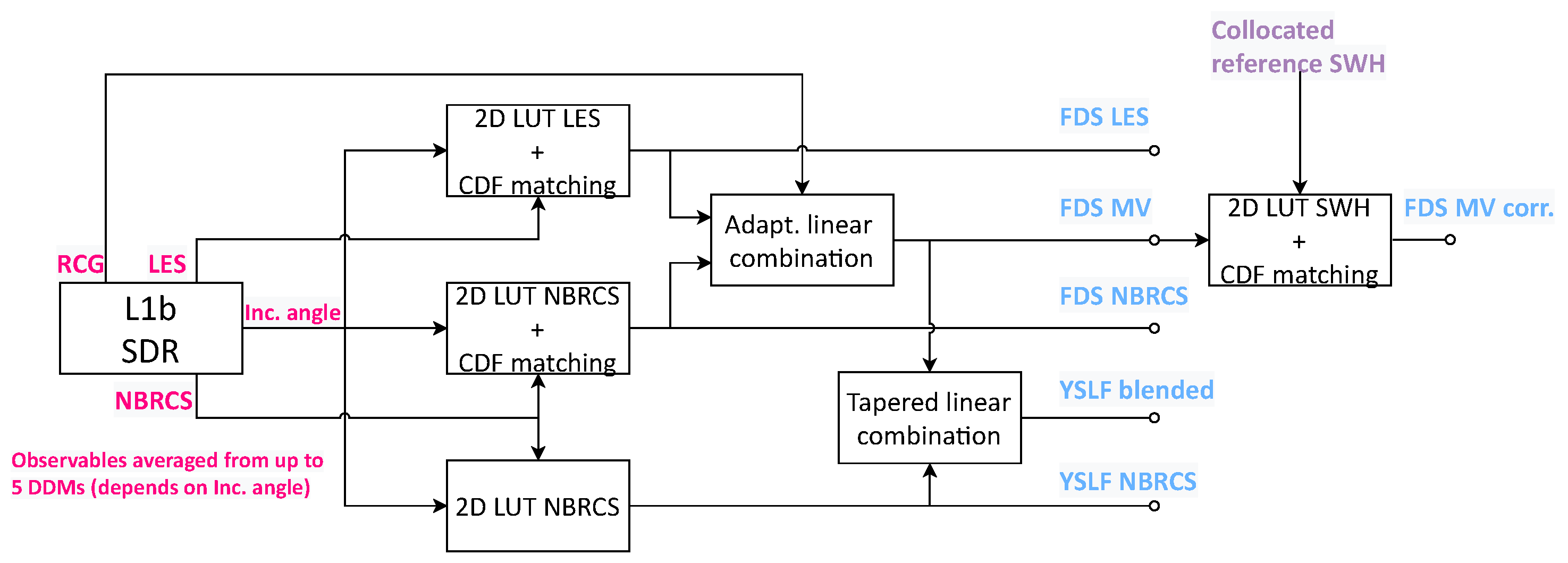
SDR Product

Figure 1 shows a conceptual sketch on how the different SDR retrievals are obtained. There are three FDS wind speed retrievals. The first, obtained from the normalized BRCS (NBRCS) (also referred in the literature as ${\sigma }^0$, DDM Average or in-short DDMA), estimated by averaging the DDM within a box of 3 delay lags x 5 Doppler bins around the specular pixel. The second, obtained with the leading edge slope (LES) of the Doppler-integrated delay waveform over the same box. The third is an adaptive linear combination of the first two and is known as the minimum variance (MV) estimate. The pair of coefficients in the linear combination are optimized so that the estimator is unbiased and its variance minimized. Both coefficients depend on an L1b derived parameter known as range-corrected gain (RCG), which, in turn, is an estimator of the signal-to-noise (SNR) ratio of the specular path before the correlation operation. The current version of the SDR product is 3.0, and until this one, the reference wind speeds used to build the FDS LUTs are obtained from the modern-era retrospective analysis for research and applications version 2 (MERRA-2) product [37]. All observables derived from the DDM are actually the averages obtained from up to 5 DDMs, depending on the incidence angle so as to have a product spatial resolution of 25 km along track. A detailed description of the FDS LUTs construction methodology can be found in [38].

After the LUT, the SDR FDS winds are debiased with respect to the same reference wind speed. The bias is a result of the systematic errors that appear when applying the LUT. The method used in the CYGNSS estimates is known as cumulative density function (CDF) matching, and consists of mapping the quantiles of the estimated wind speed CDF to those of the reference. The reference CDF is obtained using the same reference wind speed used to produce the LUT over a one-year period and across the CYGNSS coverage. This or similar debiasing techniques are widely used for the correction of climatology parameters (e.g., [39]), and, in fact, the CDF approach is also used in some of the wind speed products from the other sensors described later.

There are two YSLF wind speed retrievals. The first is also obtained from the NBRCS observable but using a LUT derived with the wind speeds produced by the NOAA/NCEP Hurricane Weather Research and Forecasting (HWRF) model [40]. The second is known as blended, and is a tapered linear combination of the former for high winds with the FDS MV for low winds. A detailed description of the YSLF LUT construction methodology can be found in [6].

This work uses the SDR 3.0 FDS MV estimate, available at the Physical Oceanography Distributed Active Archive Center (PO.DAAC) in [15].

CDR Product

In the CDR product, the L1b NBRCS and LES observables are equalized with the so-called track-wise correction. Here, track refers to the continuous acquisition between a given channel of a given CYGNSS satellite with a given GPS satellite. The same ancillary wind speeds that were used to produce the SDR LUTs are collocated in space and time with the CYGNSS observables and applied in reverse with the LUTs to obtain a new pair of NBRCS and LES observables. The original ones are corrected with a first order polynomial whose parameters are obtained from the average difference within the whole track. This correction can be understood as another wind speed debiasing technique, but the difference with respect to the CDF matching approach is that this one uses collocated wind speeds instead of modeled ones. The CDF matching is not applied in the CDR products. The motivation behind the track-wise correction is that the bias of the estimated winds not only depends on the individual GPS and CYGNSS satellites, but it also changes over time. A similar track-wise correction was first proposed by the OSWT team in [8] and is described below.

This work does not use the CDR estimates.

Product from NOAA/OSWT

The OSWT L2 product is also a reanalysis product [13]. It gives a single wind speed estimate obtained from the NBRCS observable. There are three major differences with respect to the SOC CDR estimates. First, the reference wind speeds used by the OSWT are the forecast ECMWF winds. Second, in addition to the ECMWF winds, SWH information obtained with the WW3 model is also used to equalize the NBRCS. This translates to the OSWT winds being unbiased not only with respect to the reference wind but also with respect to the reference SWH. The third major difference is that in the OSWT product, the NBRCS observable is gridded within cells of 25 × 25 km, which translates into a smaller error variance at the expense of having about three times less measurements as compared to the SOC L2 estimates. A detailed description of the algorithm can be found in [8].

The OSWT product used here is the version 1.1. It is also available through the PO.DAAC at [16].

2.1.2. ASCAT Products

The advanced scatterometer (ASCAT) [18] is the scatterometer on-board the meteorological operational (MetOp) satellites (e.g., [17]). The MetOp series consists of 3 satellites (A, B, and C) launched 12 years apart and flying in tandem mode. ASCAT is a fan-beam C-band (5.255 GHz) dual-swath scatterometer that determines the wind vector fields at the sea surface using VV polarization. Each swath is 550 km wide, and after L2 processing they are gridded with points (or nodes) separated by 25 km.

ASCAT is primarily sensitive to capillary waves due to the Bragg resonance that occurs with backscatter radars. This makes it highly sensitive to the local wind speed. The wind vector is obtained by means of a second harmonic expansion of the NRCS. The harmonic coefficients depend on the incidence angle and on the wind speed magnitude. Both coefficients are empirically obtained by fitting the harmonic expansion to collocated reference wind vectors. The current GMF is the CMOD7.n [41]. In addition, CDF matching using the same reference winds is also applied.

This work uses the wind speed L2 products of ASCAT-A and ASCAT-B built by the European Organization for the Exploitation of Meteorological Satellites (EUMETSAT) Ocean and Sea Ice Satellite Application Facility (OSI SAF) [19], both obtained also from POD.DAAC at [20] and [21], respectively.

2.1.3. Poseidon-3 Products

Poseidon-3 [23] is the altimeter on-board the Ocean Surface Topography Mission (OSTM)/Jason-2 [22] and Jason-3 (e.g., [26]) satellites. Both satellites were launched in 2008 and 2016, respectively, and have been flying in tandem mode until the deactivation of the former in October 2019. Poseidon-3 is a dual-frequency (C-band 5.3 GHz and Ku-band 13.575 GHz) nadir-looking altimeter with the goal of calculating sea surface current velocity, SWH and wind speed magnitude. It is the follow-on of the Poseidon-2 altimeter on-board the Jason-1 satellite, which was deactivated in 2013.

SWH is a direct measurement of the altimeter waveform. The wind speed is obtained with a two-parameter GMF, whose inputs are the Ku-band NRCS and the derived SWH [9]. The reason behind the inclusion of the SWH is that—similar to GNSS-R—altimeter data are sensitive not only to the ocean waves forced by the local wind, but also to the long wave roughness. It is important to emphasize here, that unlike the CYGNSS wind speed algorithms which includes SWH information, altimeters use their own derived SWH, and thus, are independent from other sensors. A calibration bias is applied to the Ku-band NRCS of Jason-2 and Jason-3 before the GMF to match them with Jason-1.

The wind speed and the SWH L2 products of Jason-2 [24] and Jason-3 [27] are obtained from the low-latency Operation Geophysical Data Record (OGDR) with a GPS based orbit and sea surface height anomalies (SSHA) calculation. Both are also available at PO.DAAC at [25] and [28], respectively.

2.1.4. AltiKa Products

The Ka band altimeter (AltiKa) [30] is a Ka-band (35.75 GHz) nadir-looking altimeter on-board the satellite with Argos and Altika (SARAL) satellite [29]. SARAL was launched in 2013 and its orbits were designed to be combined with those from Jason-2 in order to have a better SSH reconstruction.

Similar to Poseidon-3, the SWH is a direct measurement by the altimeter waveform. The wind speed is obtained with the NRCS of the Ka-band echo. Additionally, similar to Poseidon-3, the GMF uses as input both the NRCS and its own derived SWH [10]. A bias is applied to the NRCS in order to fit the derived wind distribution to the ECWMF one.

The wind speed and SWH L2 estimates are obtained from the OST XOGDR product [31], which includes an improved SARAL orbit estimation by using the SSHA differences with respect to those from Jason-2. The product is available at PO.DAAC in [32].

2.1.5. WindSat Products

WindSat [34] is the polarimetric microwave radiometer on-board the Coriolis satellite (e.g., [33]). Coriolis satellite was launched in 2003 and is still operating. WindSat receives the brightness temperature emitted by the sea surface at five different bands and at up to six different polarizations depending on the band (see Table 1), making a total of 22 polarized channels. The swath depends on the frequency band, but the most common is approximately 950 km. Its main goal is to measure sea surface wind speed and direction.

The wind speed magnitude is obtained by combining the horizontal and vertical polarizations of the different channels into a regression model whose coefficients have been empirically found using reference data. The wind speed direction is obtained from the third and fourth Stokes polarizations. The wind speed product used here is the all weather (AW) estimate, which is a blended retrieval that uses all the frequency bands and three separate algorithms to obtain winds in all weather conditions. It is included in the product daily dataset 7.0.1 [35] built by REMote Sensing Systems (REMSS) and available at [36].

2.1.6. ECMWF/WW3 Products

The ECMWF is an organization that produces global numerical weather predictions using data assimilation from meteorological observations. Among many of them are included wind speed from ASCAT and SWH from Jason-2 and AltiKa. The wind speed estimates used by the OSWT product belong to the forecast (i.e., not reanalysis) product [42]. It is also used here for comparison purposes and is available through the Institut Français de Recherche pour l’Exploitation de la MER (IFREMER) repository [43].

The WW3 model is an open-source model developed by NOAA that integrates the wave action equation [44]. It is forced by a reference wind speed and it returns several wave and sea surface spectral parameters. Among them is the SWH, defined as $H_s=4\sqrt{E}$ where E is the total (i.e., non truncated) energy of the omnidirectional (also referred as isotropical) sea surface power spectrum. The OSWT product uses the SWH from the IFREMER implementation of the WW3 model, which is driven by the forecast ECWMF winds. It is also used here for comparison purposes, and is available at [43].

2.2. Collocation Criteria

Each data product has been collocated to the coordinates of the other products, except the combinations CYGNSS 3.0 with NOAA 1.1, ASCAT-A with ASCAT-B, and Jason-2 with Jason-3. The products with a larger number of observations (hereafter named as reference) are collocated to the coordinates of the products with a smaller number of measurements (hereafter named as under-study). This means, for example, that ASCAT-A data are collocated to the coordinates of Jason-2 and not vice versa.

All the reference observations that fall within a radius of 25 km and within ±1 h window with respect to the under-study observation are averaged. Data from the full 2019 have been used for the CYGNSS SOC SDR MV estimates, ECWMF wind speeds and WW3 SWHs. For all the other products, only the first 6 months have been used, except for Jason-2 for which the data of March and April were not available. Before performing the collocation, each product has been filtered using its own quality flags, as recommended in their respective reference documents (see Table 1). For a matter of interest, the quality flags for the CYGNSS winds (both SOC SDR MV and OSWT) is given by the field sample_flags.

The collocation results of ASCAT-A and ASCAT-B have been combined in the same performance metrics, as both were found to have nearly identical performance relative to each of the other products. Similarly, the results from Jason-2 and Jason-3 have also been combined.

AltiKa wind speeds and SWHs show some anomalies at large wind speeds that are not flagged in their quality flags. Thus, the analysis metrics using this sensor are degraded. However, these anomalies will serve later to better understand the correlation between differences. More details concerning this issue are provided later.

2.3. LUT Construction

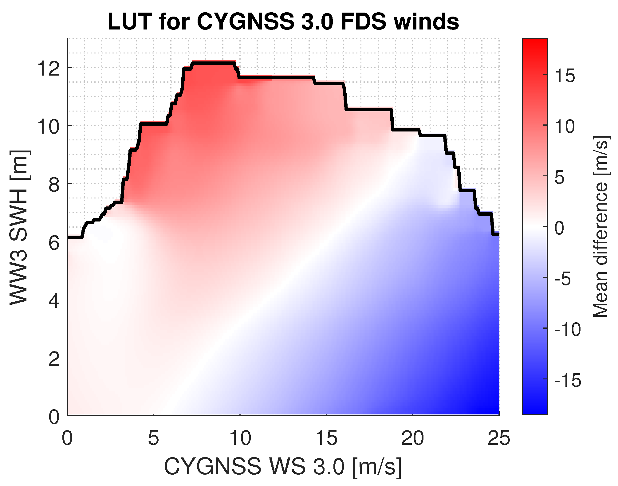
The correcting LUT is built using the CYGNSS SDR 3.0 FDS MV estimate as the winds to be corrected, the forecast ECMWF winds as the reference modeled winds, and the SWH from the WW3 model as the collocated reference SWH. Each entry in the LUT is the mean difference between the ECMWF reference wind speed and the CYGNSS estimate for a particular combination of ECMWF wind speed and SWH. The LUT presented here has been built from data over the full 2019 year. A LUT built using the odd months and tested using the even months (in order to include the annual seasonality) shows comparable performance.

The LUT is built as follows. First, the CYGNSS winds and the WW3 SWH are binned into rectangular cells. Different cell resolutions have been tried using combinations of 0.05, 0.1, 0.25, and 0.5 in both, m/s for wind speed and m for SWH. A small cell can lead to noisy estimates if the number of observations in the cell is not large enough. A large cell may indeed reduce the overall bias of the observations within the cell, but it may also translate into a large deviation in the corrected winds. After a trial-and-error process, a uniform 0.1 m × 0.1 m/s cell has been found to show the best results among the considered configurations. Using all CYGNSS/ECMWF wind speed matchups within the cell, their mean difference (ECMWF-CYGNSS) is computed. The median has also been considered and it shows a similar performance if the number of observations within the cells is sufficiently large. Next, the LUT is smoothed and any missing gaps are populated using a weighted moving average 2D window. Different window sizes (combinations of 0.5, 1.5, 2.5 m and m/s) and types (triangular or Bartlett, Welch, Hann or Hanning, and truncated Gaussian) have been tried. The best performance among the considered cases is obtained using a triangular window of size 2.5 m/s × 2.5 m. Finally, a second smoothing has been done using two 1D low-pass filters applied iteratively in each dimension. These filters are necessary to smooth the LUT at the edges, however, using a large number of iterations would lead to new artificial biases across the whole table. After a trial-and-error process, two smoothing iterations in each dimension using a Gaussian filter have been chosen. The difference between this smoothing and that using the 2D window is that the latter is done over the number of observations within each cell, while the former is applied over the cells. The SWH correction is applied to the uncorrected retrieved wind speed as a simple additive bias correction given by

$$W{S}_c=W{S}_u+\mathrm{LUT}(W{S}_u,SWH),$$

(1)

where $W{S}_c$ is the corrected retrieved wind speed, $W{S}_u$ is the uncorrected wind speed, and $SWH$ is the reference significant wave height.

The LUT is presented in Figure 2. The table is not defined outside the black line, as the number of samples in these cells was not statistically significant to compute the mean difference. The correction of the CYGNSS winds where the LUT is not defined is done by interpolating the table using a 2D linear interpolation. Three regimes can be observed: one dominated by a negative bias, one dominated by a positive bias and a zero-bias line. In the first case, the GMF overestimates the wind speed. This happens because the SWH is larger than the average one for that particular reference wind speed. This translates into a smaller NBRCS, which, in turn, translates into a larger wind speed estimated by the GMF. In the second case the opposite happens. The GMF underestimates the wind speed because the SWH is smaller than the average one, resulting in a larger NBRCS, and therefore a smaller estimated wind speed. In the zero-bias line, the retrieved winds by the GMF are not corrected, as this combination of reference winds and reference SWHs is the typical one.

After the LUT, a wind speed CDF matching is applied using modeled ECMWF winds. This is performed because this LUT is a correction tool with respect to only the SWH. However, the CYGNSS wind speed bias depends also on the true wind speed. The OSWT product handles this by using a 3D GMF that uses both collocated SWH and wind speeds. However, here, it is desired to build a product as independent as possible from other external wind speed sources.

2.4. Performance Analysis Metrics

The analysis tools used to evaluate performance of the retrieved wind speed are the mean absolute difference (MAD) (not to be confused with the mean absolute deviation), the root mean square difference (RMSD) between the retrieved and reference wind speeds, and the Pearson correlation coefficient $\rho$. They are defined as:

$$\begin{array}{cc}\hfill \mathrm{MAD}& =\frac{1}{M}\sum \left|D_{rs}\right|,\hfill \end{array}$$

(2a)

$$\begin{array}{cc}\hfill \mathrm{RMSD}& =\sqrt{\frac{1}{M}\sum D_{rs}^2},\hfill \end{array}$$

(2b)

$$\begin{array}{cc}\hfill \rho & =\frac{cov\left(W{S}_r,W{S}_s\right)}{{\sigma }_{W{S}_r}{\sigma }_{W{S}_s}},\hfill \end{array}$$

(2c)

where M is the number of matched observations, $D_{rs}=W{S}_r-W{S}_s$ is the difference between both wind speeds, and ${\sigma }_{W{S}_r}$ and ${\sigma }_{W{S}_s}$ are the standard deviation of the reference and under-study winds, respectively. The overall bias is not used because, as will be shown, in some cases is negative for low reference wind speeds and positive for large reference wind speeds. As a result, negative biases can compensate for positive biases, resulting in the overall bias being close to zero. Thus, it is not a good estimator of the average distance from the one-to-one line.

One concern with this type of correction algorithm is the possibility that ECMWF wind speeds might contaminate those of the corrected CYGNSS. Ideally, the SDR product should be as independent as possible from other wind speed products. However, the ECMWF winds can leak into the CYGNSS product in two different ways. First, from the systematic biases that may appear when building the LUT. Second, from the collocated SWHs, as they are themselves obtained from the ECMWF wind speeds. The possible leakage is studied using the Pearson correlation coefficient between the difference of the ECMWF wind speeds and the wind speeds from a reference $D_{s_{1}r}=W{S}_r-W{S}_{s_1}$ and the difference between the corrected CYGNSS winds and the same reference winds $D_{s_{2}r}=W{S}_r-W{S}_{s_2}$:

$${\rho }_a=\frac{cov\left(D_{s_{1}r},D_{s_{2}r}\right)}{{\sigma }_{D_{s_{1}r}}{\sigma }_{D_{s_{2}r}}},$$

(3)

where ${\sigma }_{D_{s_{1}r}}$ and ${\sigma }_{D_{s_{2}r}}$ are the standard deviation of the two differences. Note that this metric requires a triple collocation. The idea behind this tool is to see if when the ECMWF and the reference winds are different, this same difference is also seen with CYGNSS, or otherwise the differences are uncorrelated.

3. Results

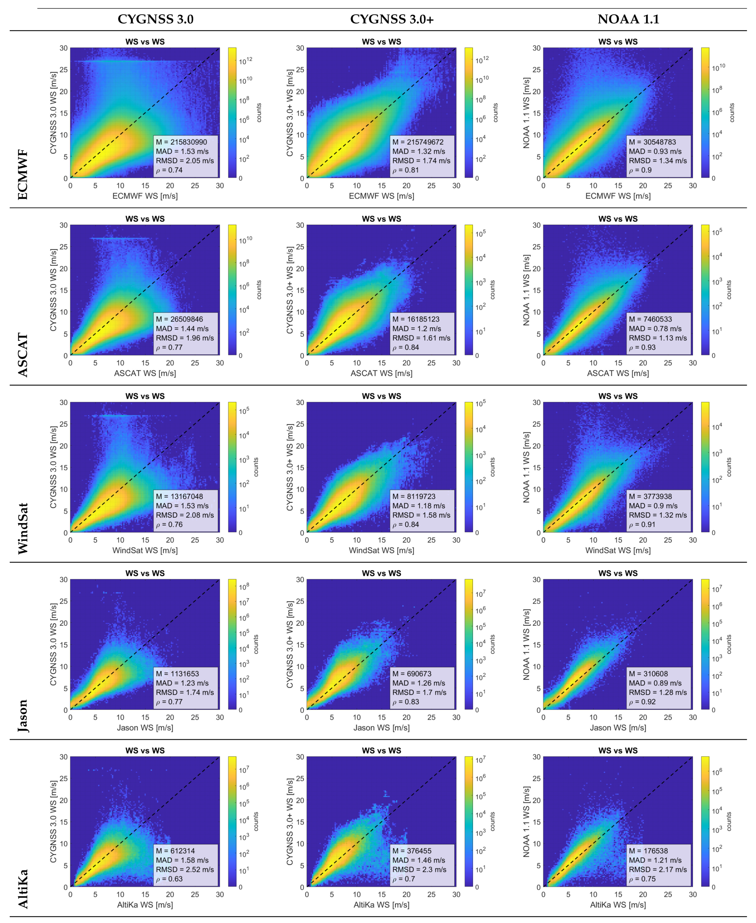
3.1. Overall Performance

Table 3. Wind speed performance metrics between different sensors and ECMWF, and among the sensors. The wind speed products from the rows are collocated to the coordinates of the products from the columns. N is the total number of observations of a given product and M is the number of matched observations. ASCAT refers to the combined results from ASCAT-A and ASCAT-B (i.e., not to the results using a triple collocation). Similary, Jason refers to the combined results from Jason-2 and Jason-3.

		Matched to
		CYGNSS 3.0 N = 354,642,211	CYGNSS 3.0+ N = 354,642,211	NOAA 1.1 N = 49,835,011	ASCAT N = 177,268,029	WindSat N = 53,424,047	Jason N = 14,067,639	AltiKa N = 6,919,763
Matched from	ECMWF	M = 215,830,990 MAD = 1.53 RMSD = 2.05 $\rho$ = 0.74	M = 215,749,672 MAD = 1.32 RMSD = 1.74 $\rho$ = 0.81	M = 30,548,783 MAD = 0.93 RMSD = 1.34 $\rho$ = 0.90	M = 114,455,219 MAD = 0.77 RMSD = 1.05 $\rho$ = 0.96	M = 55,333,269 MAD = 0.89 RMSD = 1.23 $\rho$ = 0.95	M = 7,691,627 MAD = 1.09 RMSD = 1.46 $\rho$ = 0.93	M = 3,785,627 MAD = 1.24 RMSD = 2.04 $\rho$ = 0.84
	ASCAT	M = 26,509,846 MAD = 1.44 RMSD = 1.96 $\rho$ = 0.77	M = 16,185,123 MAD = 1.20 RMSD = 1.61 $\rho$ = 0.84	M = 7,460,533 MAD = 0.78 RMSD = 1.13 $\rho$ = 0.93	X	M = 1,028,086 MAD = 0.98 RMSD = 1.34 $\rho$ = 0.96	M = 2,951,055 MAD = 0.87 RMSD = 1.23 $\rho$ = 0.96	M = 585,153 MAD = 1.02 RMSD = 1.74 $\rho$ = 0.90
	WindSat	M = 13,167,048 MAD = 1.53 RMSD = 2.08 $\rho$ = 0.76	M = 8,119,723 MAD = 1.18 RMSD = 1.58 $\rho$ = 0.84	M = 3,773,938 MAD = 0.90 RMSD = 1.32 $\rho$ = 0.91	X	X	M = 1,250,462 MAD = 0.85 RMSD = 1.12 $\rho$ = 0.97	M = 2,000,662 MAD = 1.01 RMSD = 1.80 $\rho$ = 0.86
	Jason	M = 1,131,653 MAD = 1.23 RMSD = 1.74 $\rho$ = 0.77	M = 690,673 MAD = 1.26 RMSD = 1.70 $\rho$ = 0.83	M = 310,608 MAD = 0.89 RMSD = 1.28 $\rho$ = 0.92	X	X	X	M = 67,370 MAD = 0.93 RMSD = 1.61 $\rho$ = 0.92
	AltiKa	M = 612,314 MAD = 1.58 RMSD = 2.52 $\rho$ = 0.63	M = 376,455 MAD = 1.46 RMSD = 2.30 $\rho$ = 0.70	M = 176,538 MAD = 1.21 RMSD = 2.17 $\rho$ = 0.75	X	X	X	X

presents the metrics defined in (2). They are obtained using the whole range of wind speeds and SWHs, and all the available data (see Section 2.2). The metrics between the ECMWF and the sensors other than CYGNSS, and those among the sensors themselves, are given for reference purposes. The RMSD and the correlation coefficient are also presented as an image matrix in Figure 3 for a better illustration.

The error metrics of the CYGNSS wind speeds with respect to all reference winds have improved after the correction. In particular, the improvement with respect to the ECMWF wind speeds is MAD: 1.53 m/s → 1.32 m/s, RMSD: 2.05 m/s → 1.74 m/s, and $\rho$: 0.74 → 0.81. These new metrics are worse than those from the OSWT product (MAD = 0.93 m/s, RSMD = 1.34 m/s, $\rho$ = 0.90). However, it is important to remember that OSWT is a gridded product with additional averaging performed of individual samples within each grid cell. This improves the precision of each reported product but at the expense of reducing the number of measurements (approximately by a factor of 3).

The error metrics of the same CYGNSS products with respect to either ASCAT or WindSat are similar to or even better than those using the ECMWF wind speeds as reference. This can be explained by the fact that the wind speeds given by ASCAT and WindSat are actual measurements, as opposed to the ECMWF data which are the result of a model. Additionally, the large swaths of the ASCAT and WindSat sensors allow the computation of the collocated reference wind speed using several measurements (see Section 2.2).

3.2. Performance with Respect to Reference Wind Speeds

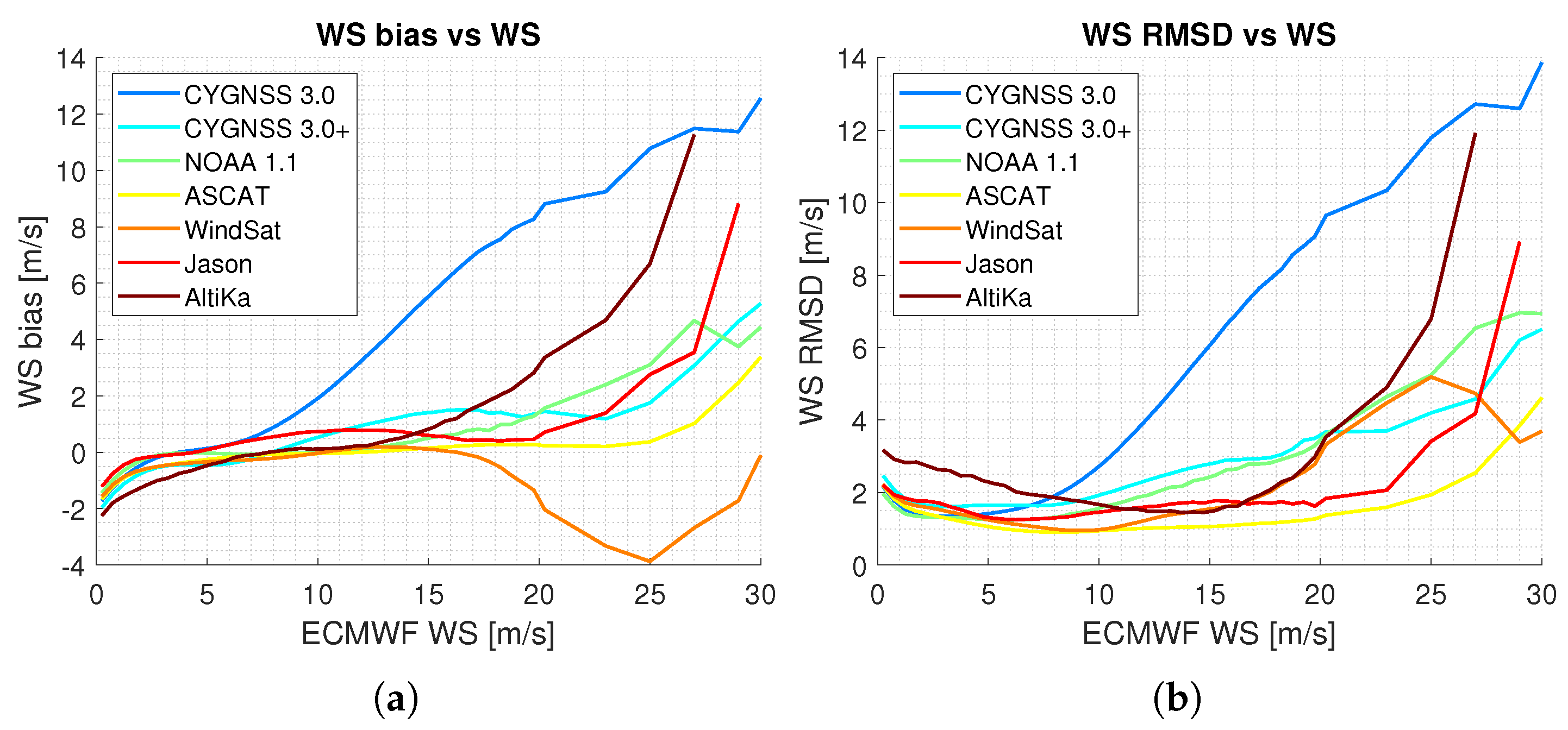
Figure 4 shows the 2D histograms of the CYGNSS wind speeds vs different reference wind speeds. The behavior of the enhanced CYGNSS wind speed vs the ECMWF wind speeds has improved across the whole dynamic range of ECMWF wind speeds, but more noticeably in two regimes. First, the large dispersion at high CYGNSS wind speeds (>15 m/s) for moderate ECMWF wind speeds (5 m/s–15 m/s) is reduced. Second, the saturation of CYGNSS wind speeds around 10 m/s disappears and the sensitivity to larger wind speeds is improved. The overall dispersion is also reduced (especially at low wind speeds) when using the wind speeds of ASCAT or WindSat as reference.

The performance against the Jason altimeters shows that Jason underestimates the low wind speeds (<2.5 m/s) with respect to CYGNSS. Additionally, few mutual observations of large wind speeds have been obtained. AltiKa behaves similarly to Jason except that the low wind speeds are truncated and it presents anomalies for wind speeds above 15 m/s. For these two reasons, the performance metrics using AltiKa are in general worse.

The overall performance of the OSWT winds relative to any of the reference winds is better than the corrected winds. However, two issues can be seen. First, there is still a dispersion for reference winds between 5 m/s and 10 m/s, which is no longer present in the corrected version. Second, it shows almost no sensitivity to reference winds above 20 m/s, unlike the corrected version.

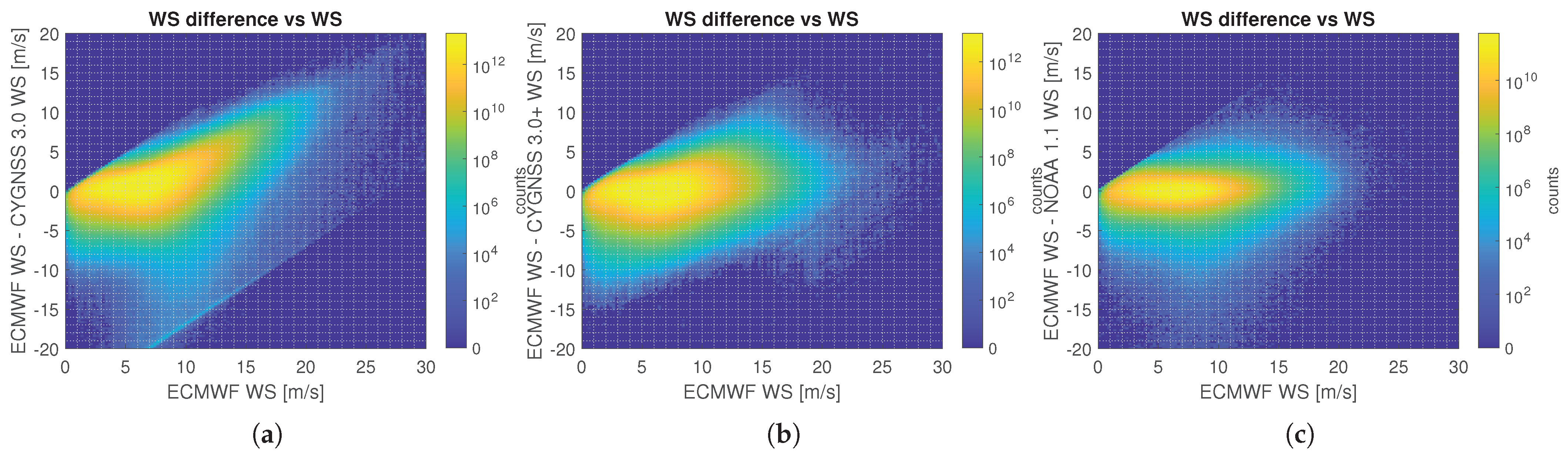
Figure 5 shows the 2D histograms of the difference between the CYGNSS wind speeds and the ECMWF wind speeds against the same ECMWF winds. The original CYGNSS 3.0 underestimates, with a similar variance, the wind speed for low reference winds. Around 2.5 m/s, the bias changes sign and together with the variance they both increase significantly with increasing reference wind speed. The corrected CYGNSS wind speed shows a much smaller error dependence on the reference wind speed. This result is important because although the inclusion of SWH in the correction presented here acts as a wind speed debiasing with respect to the SWH, a debiasing and a reduction in the variance with respect to the reference wind speed is also observed. The NOAA product also shows a very small error dependence on the reference wind speed, however, it exhibits some outliers at moderate reference wind speeds (5 m/s–10 m/s) that are no longer observed in the SWH correction estimate.

Figure 6a,b shows the bias and the RMSD versus the reference ECMWF winds, respectively, and include also the performance of the other sensors. It is easier to see now that the corrected CYGNSS bias and the RMSD for large reference wind speeds have been drastically reduced. The RMSD of the corrected CYGNSS is now almost flat around 2 m/s for reference wind speed below ≈11 m/s. The OSWT estimate follows a similar trend. The performance of ASCAT and WindSat are, in general, the best, however all the sensors diverge with respect to ECMWF (and also among them) for large wind speeds (>20 m/s). Three possible reasons are given here. First, estimates of large wind speeds are in general less accurate. Second, each sensor has a different resolution, i.e., the average area over which a single measurement is sensitive. Third, large wind speeds typically decorrelate faster in time and in space compared to the lowest ones. In other words, the performance at high wind speeds may differentiate not only because the individual estimates are inherently less accurate, but also as a result of the collocation.

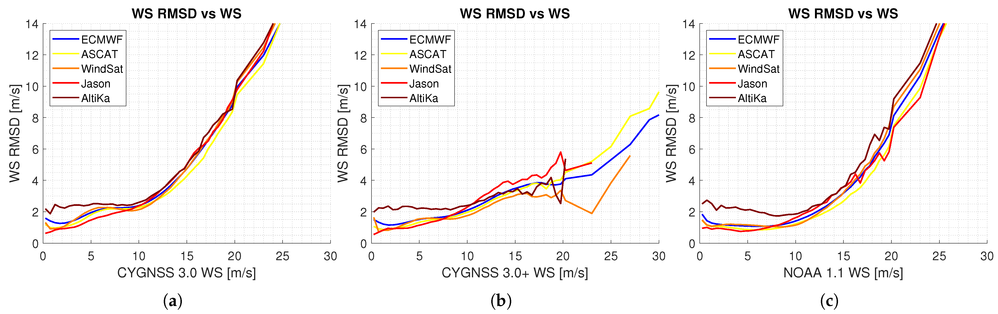
A similar analysis to Figure 6b is done in Figure 7 but using the CYGNSS estimates as reference wind speeds. Although the former figure shows the RMSD of CYGNSS when estimating a given wind speed, the second shows the RMSD of a given CYGNSS wind speed. The RMSD of the ECMWF winds when the original CYGNSS winds are the reference winds is worse than the other way around, a fact that can also be deduced from the top-left plot in Figure 4. The projection of dispersion in the vertical axis for a given horizontal wind speed is much larger than vice versa. However, when the corrected CYGNSS winds are the reference winds, the RMSD of the ECMWF winds is similar to the other way around, a fact that can be also deduced from the symmetry in the top-center plot in Figure 4. When the NOAA product is the reference, the RMSD of the ECMWF winds is almost constant at ≈1.5 m/s for wind speeds smaller than ≈10 m/s, but it increases considerably for larger wind speeds.

3.3. Performance with Respect to Reference SWHs

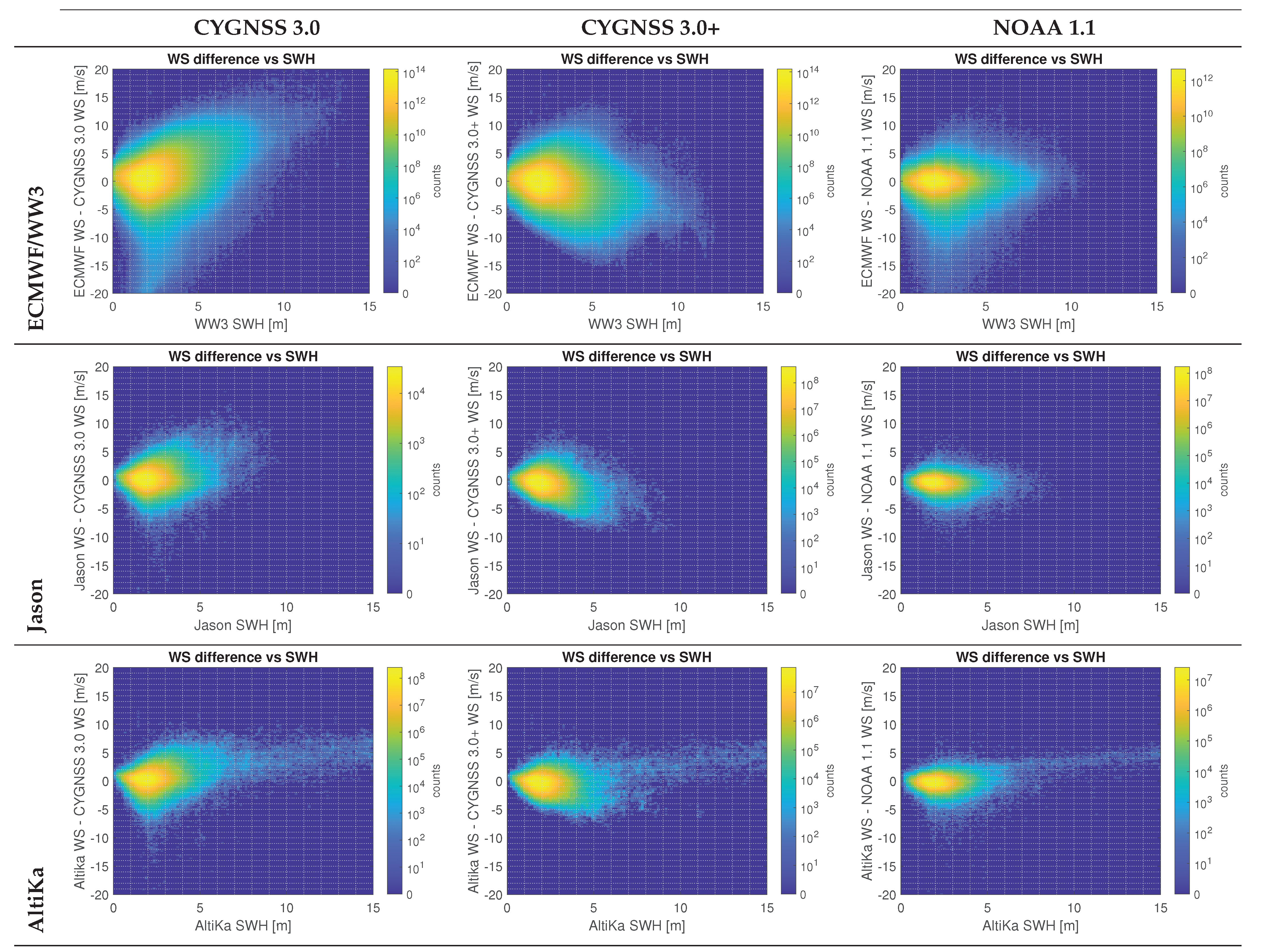
Figure 8 shows the histograms of the difference between the CYGNSS wind speeds and different reference wind speeds against the SWH given by the same references. Note first the large differences for large AltiKa SWHs, as a result of the abnormal behavior of this sensor, described previously. The dependence of the original CYGNSS wind speed error with respect to the SWH can be characterized by two different regimes. First, large positive wind speed biases are observed for moderate reference SWHs (1 m–4 m). Second, large negative wind speed biases are observed for large SWHs (>5 m). These behaviors disappear in the corrected version, however, a moderate variance and a bias (now with a change of sign) are still present and are larger than would be expected after the correction. This is so because these results also incorporate the CDF matching after the LUT correction. The CDF matching does not consider the dependence of the PDF winds to the SWH, which results into a new error dependence on the SWH. Using a 2D CDF matching which includes both modeled reference wind speeds and SWHs may be a solution to this problem, and will be considered in future work, in a manner similar to using the joint wind speed and SWH PDF proposed in [7]. The NOAA product is instead pretty much independent of the SWH, except that it still presents the outliers for moderate SWHs.

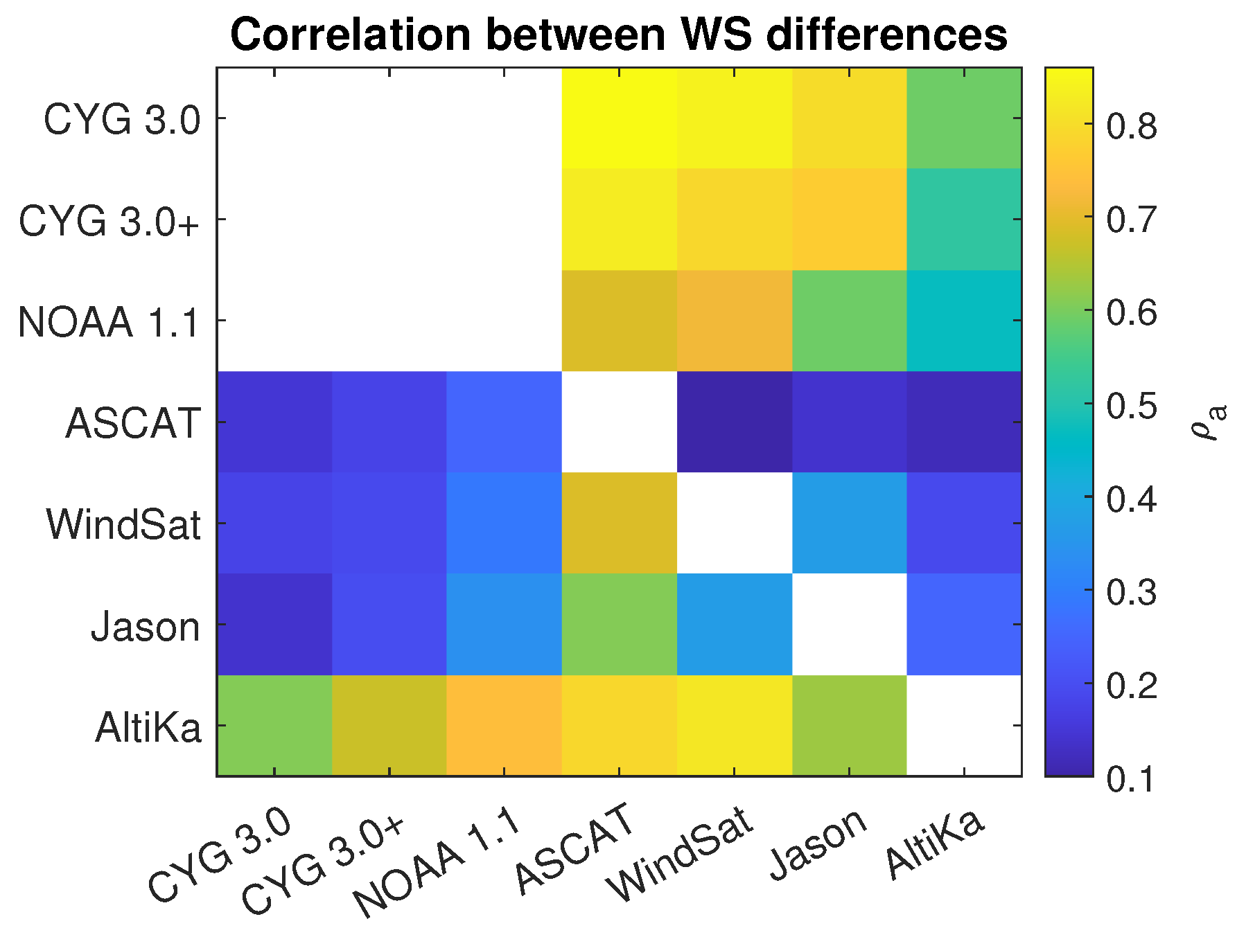
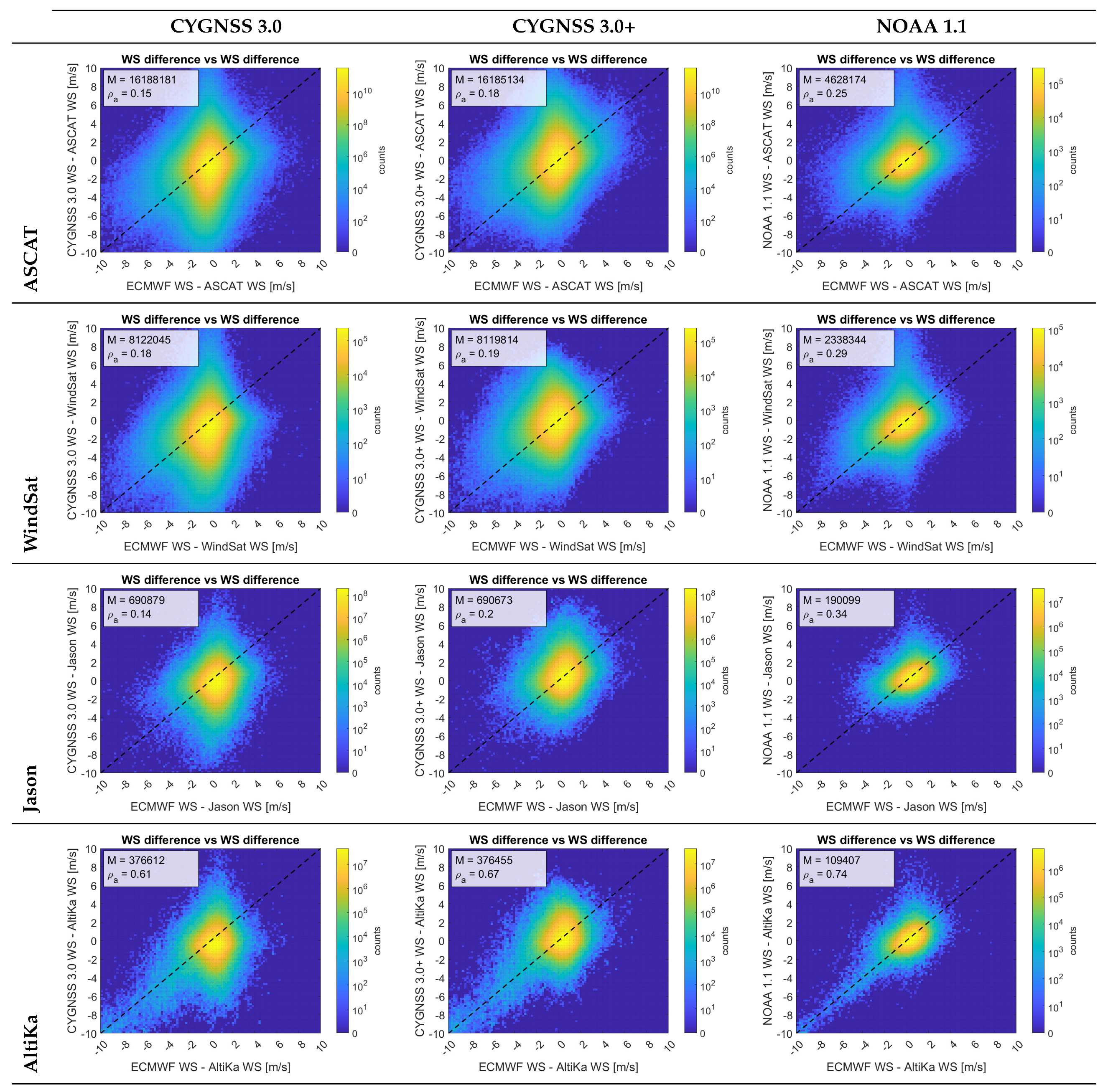
3.4. Analysis of the Correlation between the Wind Speed Differences

Table 4. Correlation between the wind speed difference of ECMWF wrt a reference sensor (rows) and the WS difference of another sensor (columns) wrt the same reference sensor. N is the total number of observations of a given product and M is the number of matched observations. ASCAT refers to the combined results from ASCAT-A and ASCAT-B (i.e., not to the results using a quadruple collocation). Similarly, Jason refers to the combined results from Jason-2 and Jason-3.

		CYGNSS 3.0 N = 354,642,211	CYGNSS 3.0+ N = 354,642,211	NOAA 1.1 N = 49,835,011	ASCAT N = 177,268,029	WindSat N = 53,424,047	Jason N = 14,067,639	AltiKa N = 6,919,763
Reference	CYGNSS 3.0	X	X	X	M = 16,188,181 ${\rho }_a$ = 0.86	M = 8,122,045 ${\rho }_a$ = 0.84	M = 690,879 ${\rho }_a$ = 0.80	M = 376,612 ${\rho }_a$ = 0.59
	CYGNSS 3.0+	X	X	X	M = 16,185,134 ${\rho }_a$ = 0.83	M = 8,119,814 ${\rho }_a$ = 0.79	M = 690,673 ${\rho }_a$ = 0.77	M = 376,455 ${\rho }_a$ = 0.52
	NOAA 1.1	X	X	X	M = 4,628,174 ${\rho }_a$ = 0.69	M = 2,338,344 ${\rho }_a$ = 0.72	M = 190,099 ${\rho }_a$ = 0.59	M = 109,407 ${\rho }_a$ = 0.47
	ASCAT	M = 16,188,181 ${\rho }_a$ = 0.15	M = 16,185,134 ${\rho }_a$ = 0.18	M = 4,628,174 ${\rho }_a$ = 0.25	X	M = 552,349 ${\rho }_a$ = 0.10	M = 1,631,612 ${\rho }_a$ = 0.14	M = 291,310 ${\rho }_a$ = 0.12
	WindSat	M = 8,122,045 ${\rho }_a$ = 0.18	M = 8,119,814 ${\rho }_a$ = 0.19	M = 2,338,344 ${\rho }_a$ = 0.29	M = 552,349 ${\rho }_a$ = 0.69	X	M = 703,764 ${\rho }_a$ = 0.37	M = 1,137,616 ${\rho }_a$ = 0.19
	Jason	M = 690,879 ${\rho }_a$ = 0.14	M = 690,673 ${\rho }_a$ = 0.20	M = 190,099 ${\rho }_a$ = 0.34	M = 1,631,612 ${\rho }_a$ = 0.61	M = 703,764 ${\rho }_a$ = 0.37	X	M = 36,060 ${\rho }_a$ = 0.25
	AltiKa	M = 376,612 ${\rho }_a$ = 0.61	M = 376,455 ${\rho }_a$ = 0.67	M = 109,407 ${\rho }_a$ = 0.74	M = 291,310 ${\rho }_a$ = 0.79	M = 1,137,616 ${\rho }_a$ = 0.82	M = 36,060 ${\rho }_a$ = 0.63	X

shows the correlation between the wind speed differences defined in Equation (3). They are also shown as an image matrix in Figure 9 for illustration purposes. A large correlation can occur for two reasons. First, one of the three references is very different from the other two, regardless of whether these two are in good agreement or not. This is for example the case of the very large correlations observed when AltiKa is one of the sensors or when the CYGNSS estimates are the common reference. A large correlation may be also the result of a high degree of coupling between two references with respect to the other one. This is the correlation of interest here.

The correlations of the original CYGNSS 3.0 are 0.15 for ASCAT, 0.18 for WindSat and 0.14 for Jason. These moderate values are believed to be a result of the first reason. After the correction, the values increase to 0.18 for ASCAT, 0.19 for WindSat, and 0.20 for Jason. These slight increments may be due to the fact that the correction gives sensitivity to large winds, and that said winds follow the ECMWF winds more than the winds of the other sensors. However, it is still safe to assume that the overall leakage of the ECMWF winds to the corrected CYGNSS winds is small. The NOAA estimate, however, presents larger correlations: 0.25 for ASCAT, 0.29 for WindSat and 0.34 for Jason, which may be the result of a higher degree of coupling with the ECMWF winds, due to the latter being used in NOAA’s track-wise correction algorithm.

As a qualitative visual interpretation of the numbers given above, Figure 10 shows the histogram of one difference against the other. It can be observed that the error ellipse of the NOAA estimate is indeed tilted as a result of a larger correlation, whereas it is not tilted as much for the corrected version developed here. A high degree of coupling between ECMWF and CYGNSS estimates when AltiKa is the reference sensor can also be observed.

4. Discussion

Previously, two different approaches have been proposed that use SWH information to improve the GNSS-R wind speed retrievals. First, a Bayesian approach and a modeled joint-PDF of reference wind speed and SWH was tested with TDS-1 data in [7]. Second, the NOAA/OSWT approach on the use of collocated reference wind speeds and collocated reference SWHs to equalize CYGNSS L1b observables in [13]. The altimeters Jason [9] and AltiKa [10] also use SWH correction strategies for their wind speed products. However, the SWH they use is derived from their own measurements, making their wind speed estimate independent from other sources.

The LUT approach proposed here is a method that uses only collocated SWHs as reference data. The LUT has been built using CYGNSS winds below 25 m/s and reference SWHs below 13 m, since the number of observations was not statistically significant to compute the mean difference when either of the two was larger or for certain combinations of both. For these certain combinations, and for CYGNSS winds between 25 m/s and 30 m/s, the winds have been corrected by interpolating the LUT with a linear 2D interpolation. The LUT has not been analyzed for CYGNSS winds above 30 m/s (such as those found in hurricanes).

The performance of the corrected CYGNSS winds in the said regime shows an increase in the sensitivity to large wind speeds, an improvement of the overall RMSD with respect to ECMWF winds to 1.74 m/s and an increase the overall correlation with respect to the same winds to $\rho$ = 0.81. No error dependency has been found on the CYGNSS or GPS satellite, nor on the incident angle, as inequalities from these parameters have already been taken into account in the L1 corrections and in the construction of the GMF. The leakage of the ECMWF winds to the estimates is found to be negligible. It appears to be present to a greater extent in the NOAA product.

The reference winds and SWHs used to build the LUT are forecast estimates. It is then not unsafe to assume that using reanalysis estimates, such as those from the ECMWF Reanalysis v5 (ERA5) product, would lead to even better performance. However, doing so may also increase the latency of the corrected product, as the reanalysis products take longer to be available.

5. Conclusions

This article has presented a CYGNSS wind speed debiasing technique using SWH data. The method utilizes a 2D LUT correction with inputs given by the CYGNSS wind speed estimates and collocated WW3 SWH data generated with ECMWF forecast winds, followed by matching the CDF of the final retrieved wind to that of the reference winds. Although the debiasing is done with respect to the SWH, the bias and the variance of the resulting winds are also reduced with respect to collocated ECMWF winds. At the same time, the sensitivity to large wind speeds increases, and outliers that were present for moderate reference wind speeds are reduced.

The overall improvement with respect to the 3.0 version is MAD: 1.53 m/s → 1.32 m/s, RMSD: 2.05 m/s → 1.74 m/s, and $\rho$: 0.74 m/s → 0.81 m/s. The improvement is more noticeable for reference wind speeds above 10 m/s. Additionally, a similar performance is observed when either the ECMWF winds or the corrected winds are the reference winds. This is not the case when the uncorrected winds are the reference winds, in which the RSMD for large winds is much larger than when the ECMWF winds are the reference ones. To a smaller extent, this dual-behavior is also seen in the OSWT product.

The possible contamination of the ECWMF winds into the corrected ones is analyzed using the correlation between the differences of both CYGNSS winds and ECMWF winds with respect to the same common reference winds. There is a slight increase in the correlation coefficients which may be produced by the increase in sensitivity to large winds, as they match more with the ECMWF than with the other sensors.

The correction proposed here will be adapted and incorporated in a future version of SOC SDR MV winds v3.1. Such new version will include important L1 corrections, so it is expected that the final performance can be improved further. At the moment of writing, it is yet to be decided which wind speed and SWH sources will be used.