Abstract
Point cloud classification plays a significant role in Light Detection and Ranging (LiDAR) applications. However, most available multi-scale feature learning networks for large-scale 3D LiDAR point cloud classification tasks are time-consuming. In this paper, an efficient deep neural architecture denoted as Point Expanded Multi-scale Convolutional Network (PEMCNet) is developed to accurately classify the 3D LiDAR point cloud. Different from traditional networks for point cloud processing, PEMCNet includes successive Point Expanded Grouping (PEG) units and Absolute and Relative Spatial Embedding (ARSE) units for representative point feature learning. The PEG unit enables us to progressively increase the receptive field for each observed point and aggregate the feature of a point cloud at different scales but without increasing computation. The ARSE unit following the PEG unit furthermore realizes representative encoding of points relationship, which effectively preserves the geometric details between points. We evaluate our method on both public datasets (the Urban Semantic 3D (US3D) dataset and Semantic3D benchmark dataset) and our new collected Unmanned Aerial Vehicle (UAV) based LiDAR point cloud data of the campus of Guangdong University of Technology. In comparison with four available state-of-the-art methods, our methods ranked first place regarding both efficiency and accuracy. It was observed on the public datasets that with a 2% increase in classification accuracy, over 26% improvement of efficiency was achieved at the same time compared to the second efficient method. Its potential value is also tested on the newly collected point cloud data with over 91% of classification accuracy and 154 ms of processing time.
1. Introduction
The advent of Light Detection and Ranging (LiDAR) technology provides an effective way to acquire 3D spatial data in the form of point clouds. The point cloud data provide detailed geometric information that can be used to accurately and densely describe the structure of the object [1,2,3]. Since identification and analysis of a 3D LiDAR point cloud is the basis for realizing scene understanding, the 3D semantic perception of LiDAR point cloud data hold potential for many applications [4,5,6,7,8,9,10], such as topographic mapping [11,12] and automatic driving [13,14,15]. Among the various applications with respect to 3D point cloud processing, point cloud segmentation, which is a method to divide the point cloud into different homogeneous regions such that the points in the same isolated and meaningful region have similar properties, or point cloud classification aimed to realize identification of the semantic label for each point, plays a significant role for the interpretation of the LiDAR point cloud.
In recent years, with the development of deep learning [16,17,18], various deep neural networks for point cloud processing have become available and achieved impressive results in classification tasks [19,20]. An early point cloud classification network [21,22] based on a Convolutional Neural Network (CNN) used a voxelization technique to process the point cloud data. Since the convolution operation requires a structured grid, it cannot be implemented directly on point cloud data with irregular structure in 3D space. Voxelization converts the point cloud data of a discrete structure into the form of a continuous domain so that the voxelized point clouds can be directly processed by 3D convolution operations and the deep learning methods can be applied to point cloud classification through indirect means. Although this approach has shown good performance, it suffers from high memory consumption due to the sparsity of the voxels. To address this, MVCNN [23] converts 3D point clouds into a collection of 2D images, which uses 2D convolution instead of 3D convolution to reduce the number of parameters. Moreover, compared with 3D voxels, the multi-view images contain texture information of objects, which leads to better classification performance by extracting information in this way; however, this method also suffers from inefficiency due to the large number of images to be processed. As the point cloud classification technique becoming increasingly sophisticated, deep neural networks that can be directly implemented to process raw point clouds has received increased attention. PointNet [24] is a pioneering work that directly takes the unstructured point clouds. It adaptively learns features from point clouds using multilayer 1D convolution. PointNet conducts feature learning for each point without taking into account the local spatial information; thus, the local structural relationship between points cannot be captured. To overcome this issue, PointNet++ [25] applies a sampling and grouping strategy that divides the point cloud into several small local regions and then abstracts the local point cloud regions through the convolution operation layer by layer to generate a feature vector of the regions. Specifically, PointNet++ proposes a Multi-Scale Grouping (MSG) strategy to combine features from different scales of regions. Although multi-scale feature fusion enables us to capture abundant geometric information from the neighborhood for feature learning, it comes with a high computational cost; therefore, how to explore the local information efficiently for point cloud classification represents a challenging problem.
To this end, an efficient multi-scale point feature learning network for point cloud classification is proposed in this study. We developed a point cloud classification network based on the traditional encoding–decoding structure. In the network, we make use of the K-Nearest Neighbors (K-NN) approach and extend it with an expansion sampling strategy to realize efficient multi-scale feature learning. Moreover, to better represent the spatial relationship between those extracted neighboring points, both the absolute positions of all neighboring points and the relative position between points are taken into concern in feature learning.
2. Related Work
In concern of the local spatial information, available point cloud classification networks can be categorized as ball query based or K-NN based feature learning networks. Below, we briefly review the methods of each category and demonstrate the rationale for the proposed method.
2.1. Ball Query Searching Based Feature Learning Networks
Ball query is a method that sets the radius concerning the center point and then finds all points within the radius. PointNet [24] applies the ball query method to search the neighboring points and then utilizes the max-pooling which samples the maximum value in a local patch to abstract the neighborhood information as a high-level feature for the input sample. As a follow-up, PointNet++ [25] uses ball query but with different radius in searching of neighboring points. It introduces an abstraction layer to group points hierarchically and combines multi-scale local geometric details which is able to deal with the non-uniformity problem of point clouds. PointSIFT [26] is further developed based on PointNet++ and the 2D shape descriptor of Scale Invariant Feature Transform (SIFT) [27]. It proposed the Orientation-Encoding module to extract features. This module first utilizes the ball query method to search the point set in each of the eight spatial directions (adopted by SIFT descriptor) in the point cloud space, then three successive convolution layers are deployed for furthermore feature mapping. Finally, the network connects those encoded features from different spatial directions. PointConv [28] queries the neighboring points and then replaces 3D convolution with matrix multiplication and 2D convolution to ensure translation invariance and permutation invariance by sharing weights. LSANet [29] also uses a ball query skill for local points searching and a Local Spatial Aware (LSA) layer to learn the spatial distribution relationship between points and capture local geometric structures.
2.2. K-NN Searching Based Feature Learning Networks
Apart from the ball query approach, K-NN is another strategy that searches for the nearest K neighboring points for each input point to summarize its local information for feature learning. For example, RandLA-Net [30] conducts K-NN to search for the neighboring points after random sampling, and then a local feature extraction module is adopted to aggregate point features. With the rise of attention mechanisms [31,32], there have been many reported studies utilizing K-NN searching and attention mechanism to capture the important local information for input point clouds [33,34]. Among them, PCT [33] embeds transformer [35] into the framework to better capture local context between point clouds. GACNet [34] defines a novel Graph Attention Convolution (GAC) to focus on the most relevant parts of points by their dynamic learning characteristics.
For those mentioned point cloud networks, the adequate capture of 3D point local contextual information often requires increasing the radius of the ball or constructing larger K-neighborhood graphs. However, these operations make their networks inefficient in terms of the processing time and memory consumed. Especially when the attention mechanism is adopted, the amount of parameters has increased considerably though it is beneficial for the improvement of the network performance. To conquer the inefficient feature learning problem aroused by ball query or K-NN strategy when searching points within larger receptive field, our study intends to develop an efficient network for large-scale 3D LiDAR point cloud classification. Specially, a Point Expanded Grouping (PEG) strategy is introduced to increase the receptive field for feature learning of each center point and realize multi-scale learning by changing a point expansion rate efficiently. In addition, to fully characterize the local spatial relationship between points, an Absolute and Relative Spatial Embedding (ARSE) approach is adopted for comprehensive representation of the spatial relationship. The combination of these two contributions makes our network perform well on the large-scale 3D LiDAR point cloud classification task. In particular, to testify the practical use of the proposed method, a new Unmanned Aerial Vehicle (UAV)-based LiDAR point cloud dataset was collected in the Guangdong University of Technology and a training set of this newly collected dataset was manually created for model training. The proposed method is demonstrated potential value with promising classification results on this practical data.
3. Methodology
In this section, we will introduce the network structure and provide details of the feature learning process of the entire network.
3.1. Network Structure
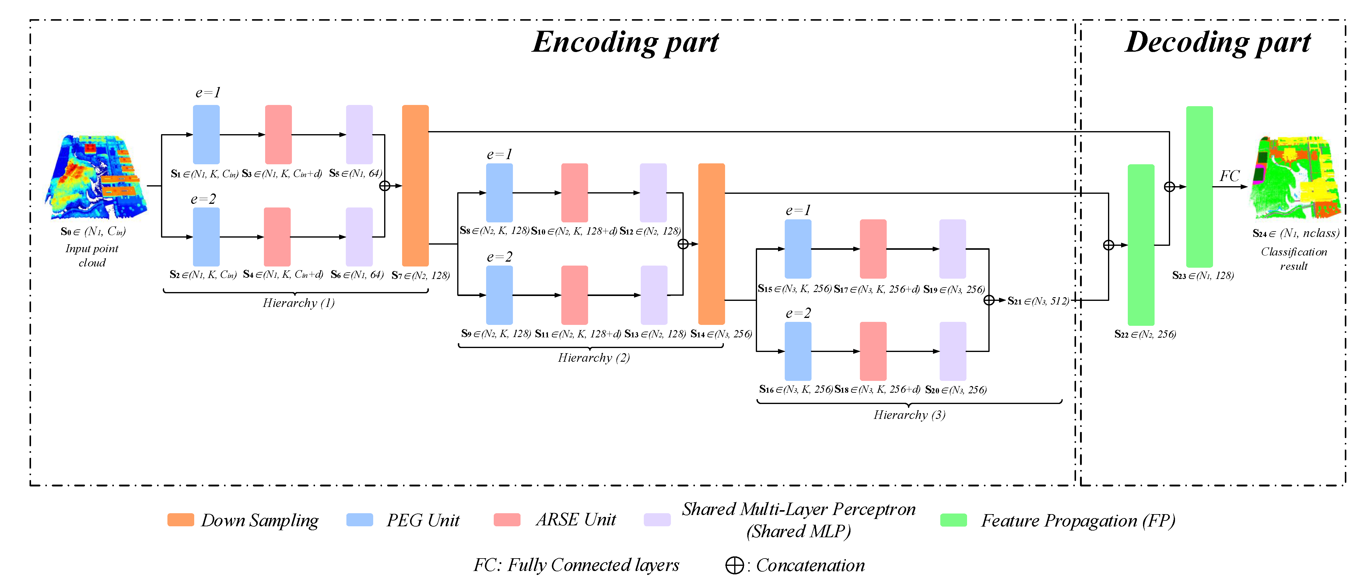
Similar to the typical point cloud classification networks [24,25], we also adopt the encoder-decoder architecture network as shown in Figure 1. Our PEMCNet includes two efficient units of PEG and ARSE to learn multi-scale point features for 3D LiDAR points. The main difference between our network and the most available point cloud classification networks is in the encoding part. This part of our network, has three multi-scale feature learning hierarchies (specifically, two scales are used in each hierarchy to construct a lightweight network) and each of them enables extraction of different scale point features through two PEG units. In addition, an ARSE unit follows each PEG unit to better represent the spatial position relationship between points. Finally, all the point features are concatenated for further feature learning. In the decoding part, it is mainly constructed by FP [25] module which up-samples the feature map via interpolation [25] and then renders fusion with the intermediate feature map from the decoding part. Finally, the FC layers are utilized for classification.
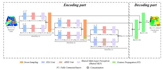
Figure 1.
Illustration of the detailed architecture of PEMCNet for large-scale point cloud classification. The encoding part is composed of PEG unit, ARSE unit and Shared MLP. The decoding components mainly consist of FP. represents the obtained feature vectors of each function unit.
3.2. Feature Learning
As shown in Figure 1, the proposed PEMCNet has three main hierarchies in the network to realize the multi-scale feature learning for the point cloud. Each hierarchy of the PEMCNet in the encoding part consists of two feature learning branches. Each branch consists of a proposed PEG unit, ARSE unit, and a commonly used Shared MLP [36] module.
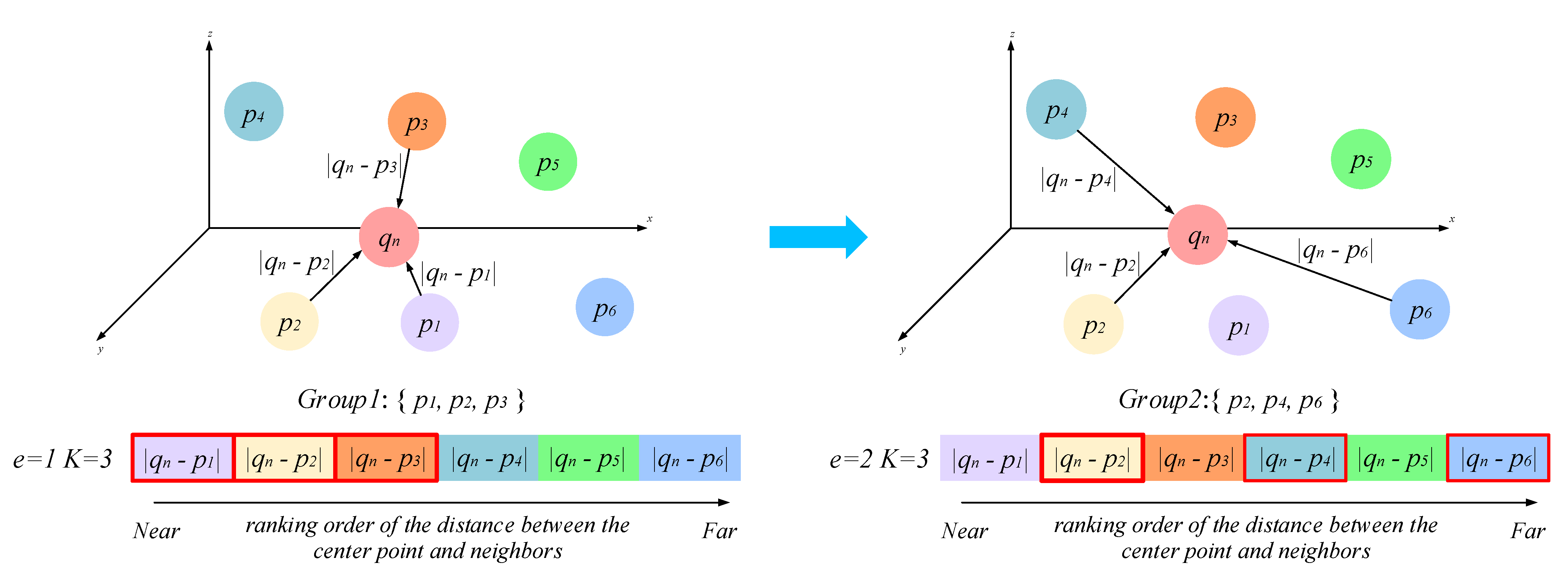
The PEG strategy adopted the network aim at finding neighboring points around the centroid at given expansion rate e. This strategy conducts simultaneous K-NN searching at different expansion rates, which prompts an efficient learning process and lightweight storage space. The two PEG units in each hierarchy are assigned different expansion rates which realize multi-scale feature learning. In each PEG unit, every input point is considered to be the center point and sparsely sampling at an expanded step will be conducted to find its neighboring points to be used for summarizing the local information. Specifically, an expansion rate parameter e is needed to realize the sparse sampling. The principle behind the PEG unit is illustrated in Figure 2. Suppose , it means that three nearest neighboring point features of the nth center point q. Likewise, the points set at the other scale will be picked instead. In this way, it can be clearly understood that the proposed PEG strategy enables enlargement of the receptive field in dense point feature learning and realize multi-scale feature learning by varying the expansion rate. It needs to be highlighted that this multi-scale searching process is without additional computation. Therefore, this is what makes the proposed network efficient.
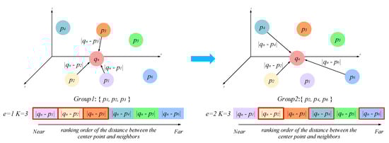
Figure 2.
Working principle of PEG unit. denotes the ith nearest neighboring point feature of the centroid . The red boxes indicate the selected point features.
Given that the input point cloud set for classification is and , where is the number of input points and represents the dimension of the original point feature which includes the x-y-z coordinates, pulse intensity and the return number of each point. It can also include RGB information of each point (depends on the specific dataset). Through a PEG unit, K neighboring points are sampled for each input point at a specific expansion rate to acquire the local point features at one scale. In each hierarchy, such as the first hierarchy, as illustrated in Figure 1, two sets of point feature vectors and will be obtained as a two-scale set of point features.
The ARSE strategy deployed in the classification network helps to better depict the spatial relationship between each centroid and its neighboring points which increases the point feature dimension of each point with more abundant spatial information. Embedding the x-y-z coordinates (absolute position) of all neighboring points in feature learning of the point cloud is argued not informative enough and the relative position between points is also significant. Therefore, after extraction of neighboring points through the PEG units, the ARSE unit works to unit information both of absolute position and the relative position between points. As shown in Figure 1, the ARSE unit is deployed following each PEG unit to encode the absolute and relative positions of the nth center point q and it’s the kth neighboring point as follows:
where is the relationship evaluation function of the proposed ARSE unit, denotes the x-y-z positions of the nth center point q, calculates the Euclidean distance and ⊕ is the feature concatenation operation which means that the dimension of the original point feature vector is expanded by splicing the absolute position and relative position information of each point. After this unit, the channel number of the point feature vector in each hierarchy will increase by d dimensions. For example, the data flow of each branch in the first hierarchy varies as: , . This in fact will benefit the entire network to learn local spatial structures better.
After local information learning through the PEG unit and ARSE unit, a three-layer Shared MLP follows to realize further feature mapping. Through this module, the extracted local point information is summarized with max-pooling operation. The number of 1D convolution kernels in three layers of the Shared MLP in the first hierarchy are 32, 32, and 64, respectively, thus the input point features through Shared MLP are learned as . (same for in the other branch). Then, the point features at two scales are spliced together and a Farthest Point Sampling (FPS) [25] algorithm is conducted at the same time to implement down-sampling, the new point feature map is learned as . The point feature learning process of the Hierarchy (2) and Hierarchy (3) is the same as Hierarchy (1). The three-layer Shared MLP structure used in those two hierarchies are and , respectively. A down-sampling operation is performed between each hierarchy. Throughout the encoding process, the point feature map obtained by each hierarchy is , , , where is the number of points after down-sampling. As can be seen that the feature dimension of per-point is increased in each hierarchy to retain more information. For the decoding part, the encoded features go through a couple of FP modules. In each FP module, the weighted average of the inverse distance between points is first calculated to find the nearest neighbor point for each centroid, so that the point feature set obtained from the previous layer can be up-sampled utilizing the nearest neighbor interpolation [25]. The feature maps obtained via up-sampling are then concatenated with the intermediate feature maps achieved with a corresponding encoding hierarchy (shown in Figure 1) for further learning with a Shared MLP. Finally, the fused point features are processed through the FC layers, where the output is a probability vector that has the length as the number of categories of the specified task, to realize point cloud classification.
3.3. Loss Function
The cross-entropy loss function is used in the training of the developed PEMCNet. This loss function is shown as follows:
where indicates the probability that the point belongs to the ith category, and represents the probability score of each point predicted by the network corresponding to the ith category. denotes the number of categories. This loss function takes the natural logarithm of the probability value and multiplies it with the true label y. Then the sum of the negative values of all products is the expected loss.
4. Experiment
In this section, we first evaluated the performance of our network on two public datasets. Then, the efficiency of the proposed method was tested on our newly collected UAV-based LiDAR point cloud dataset. Four state-of-the-art methods, Pointnet++ (MSG) [25], PoinSIFT++ [26], PointConv [28], and LSANet [29], were used as counterparts to compare with our network. The performance of the point cloud classification is verified on both aspects of accuracy and efficiency. The accuracy is evaluated in terms of mean Intersection over Union (mIoU) and overall accuracy (OA). Intersection over Union (IoU) is calculated as:
where IoU is used to evaluate the percentage of the intersection of the true value and predicted value to their union. For the point cloud classification task, a larger value of IoU means that more points are predicted as correctly classification labels. The mIoU is the average of IoU of all the categories expressed as Equation (5).
OA describes the ratio of correctly predicted points to all the test points as shown in Equation (6).
where is the number of categories, denotes the number of samples correctly determined as category i, indicates the number of samples incorrectly determined as category j from true category i. The meanings of and are the same as and .
As for efficiency evaluation, model size and forward time are utilized. The forward time was recorded with a batch size of 4 on a single RTX 2080Ti GPU, which is the same hardware environment for the implementations of other comparison approaches.
4.1. Experiments on the Public Datasets
We evaluated the proposed PEMCNet firstly on two public datasets. The first public dataset is the Urban Semantic 3D (US3D) dataset [37], which is provided by the IEEE Geoscience and Remote Sensing Society (GRSS) for the Data Fusion Contest in 2019. Each point in this airborne LiDAR point clouds dataset is described with the x-y-z coordinates, intensity, and return number. The point clouds have been manually marked as five classes of ground, high vegetation, building, water, and elevated road. The other large-scale benchmark LiDAR dataset is Semantic3D [38] which has 15 training scans and 15 test scans from a variety of urban and rural scenes. This dataset consists of 8 classes, man-made terrain, natural terrain, high vegetation, low vegetation, building, hard scape, scanning artifact, and car. The five features of this point cloud dataset are the same as that of US3D.
In the experiments, each dataset was partitioned into a training set and a validation set at the ratio of 9:1. We used the Adam optimizer for our network optimization and the momentum was set as 0.9. As for the hyper-parameter settings, the initial learning rate of our network was fixed as 0.001; the batch size was 4. The epoch was set as 201 for US3D and 500 for Semantic3D, as the latter dataset is larger with over 4 billion labeled points. The learning rate decays 0.7 for every 68720 steps on the former dataset and every 200,000 steps on the Semantic3D dataset. The number of input points in experiments with two datasets was 8192. The main hyper-parameter K in our network was fixed as K = 16 in each PEG unit, which means that 16 neighboring points of each center point were chosen for each scale feature learning in each hierarchy. Two expansion rates in each hierarchy of the encoding part were set as 1 and 2, respectively, in the experiments.
4.2. Classification Results
Table 1 presents the quantitative classification results of different approaches on the first public datasets concerning both accuracy and efficiency. It is worth noting that compared with other related neural network algorithms, our method performed the best on both aspects. As for efficiency, PEMCNet demonstrates faster classification process with fewer parameters. Specifically, the model size of our network was only 6.37 MB, which was about 14 times smaller than LSANet; this led to the fastest processing time, which is approximately a 26% increase in efficiency compared to that of the second efficient method of PointNet++ (MSG). Concerning classification accuracy, the two accuracy metrics of OA and mIoU were both observed with the highest values among all the results. The mIoU of our method increased by 2% and OA increased by 1% upon that achieved by the method ranked in second place. The improved accuracy could be observed from the detailed increase in each category summarized in Table 2. It can be seen that every category can be identified by our method with higher accuracy, the category of water was especially better classified.

Table 1.
Quantitative classification performance of different networks on US3D dataset.
Table 2.
Classification accuracy of each class of different networks on US3D dataset in terms of IoU (%).
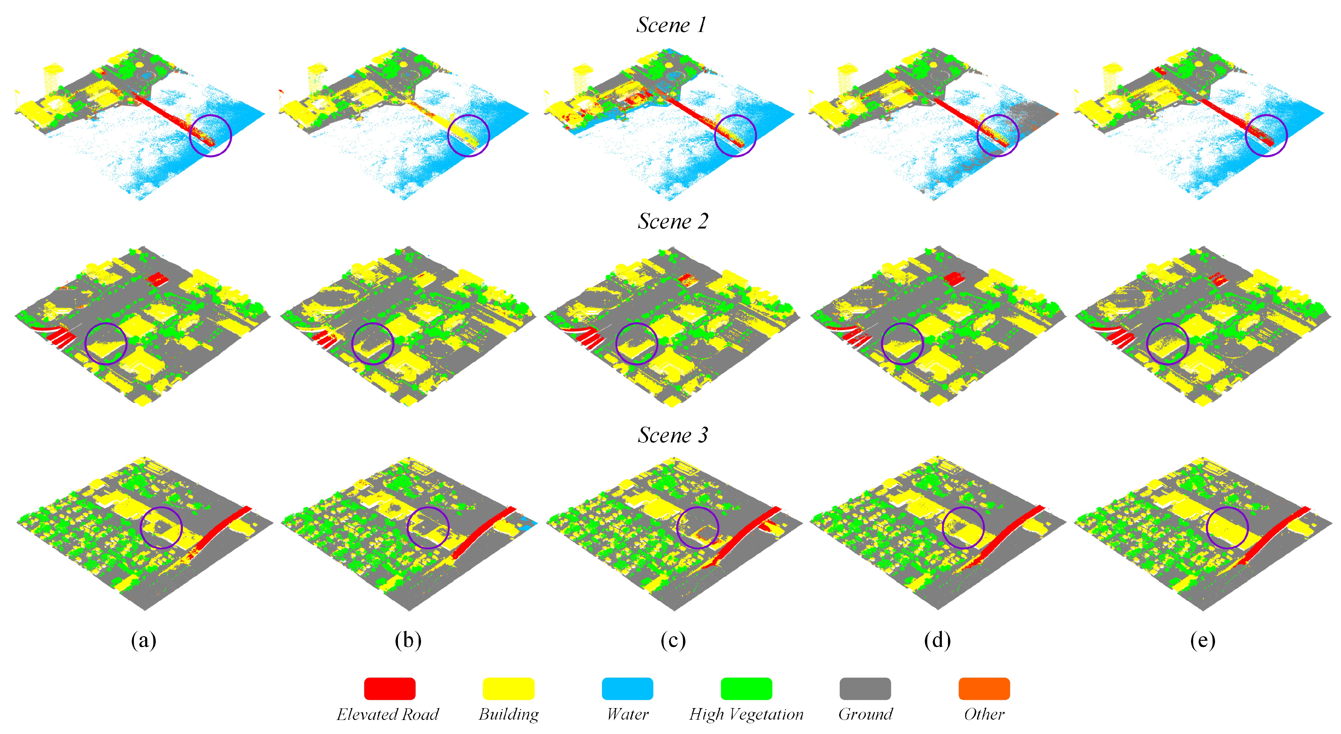
Figure 3 qualitatively illustrates the classification results achieved by five approaches on the three test subsets of the US3D dataset. It clearly shows that our method achieved smoother classification results, in particular, in the circle region of interest. In the intersection region between different classes, our approach displays better results. Fewer misclassified points were observed with the proposed method than the other methods. For example, the subfigures in the first row of Figure 3 show that the elevated road and water were clearly classified with our method. This is in fact in accordance with the classification results presented in Table 1.
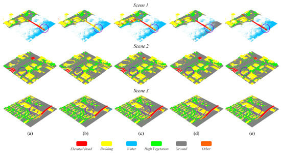
Figure 3.
Classification results of five different approaches on the test set of US3D dataset: (a) PointNet++ (MSG); (b) PointSIFT; (c) PointConv; (d) LSANet; (e) PEMCNet.
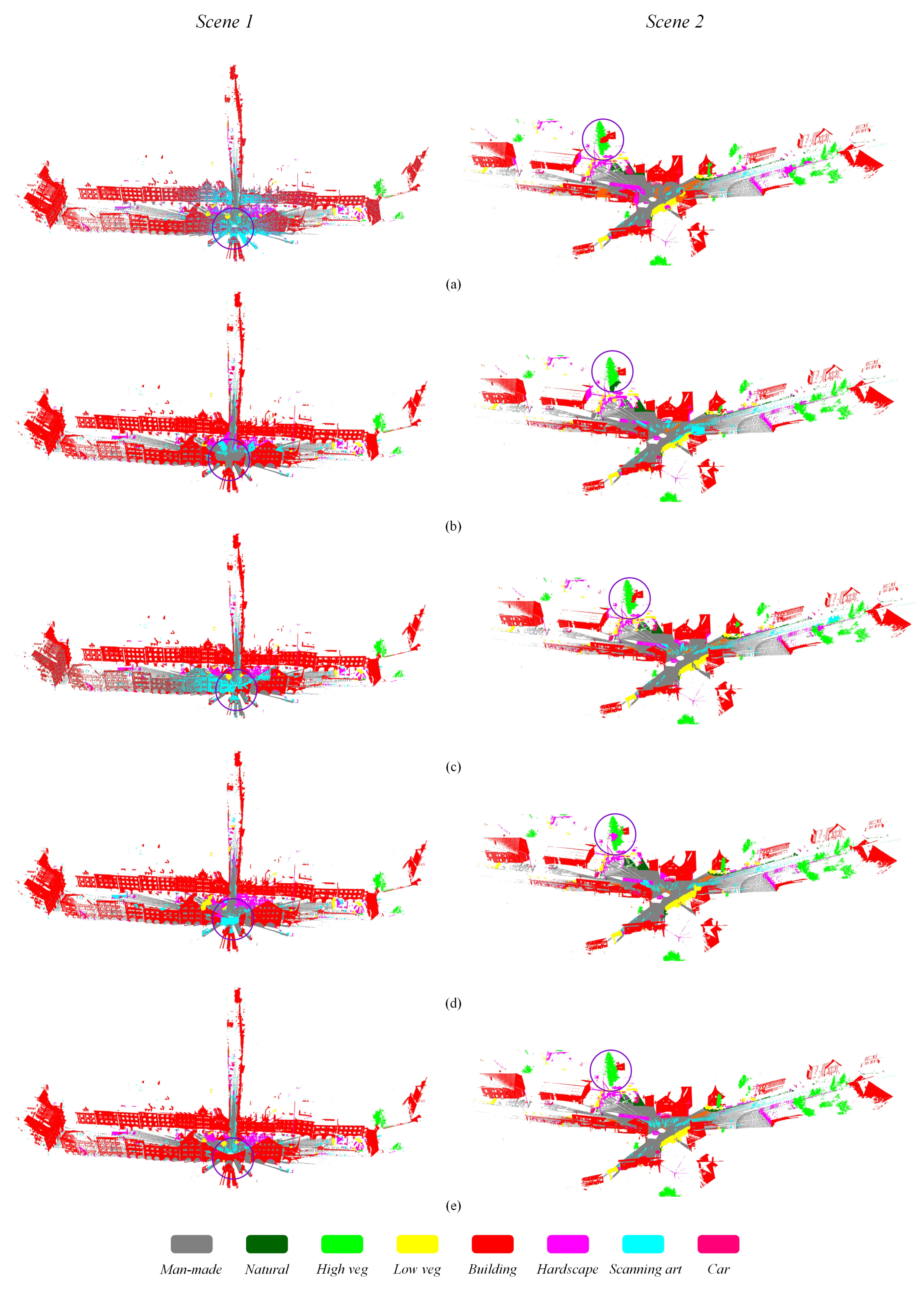
Table 3 shows the quantitative classification result of different approaches on the second public dataset of semantic3D. In accordance with what has been observed from experimental results on the US3D dataset, the same conclusion can be drawn from the results of this dataset. PEMCNet also achieves the best classification accuracy and efficiency. Over 26% improvement in efficiency was achieved compared to that of the second efficient method of PointNet++ (MSG). Compared with LSANet, the classification accuracy increased by over 2% in terms of both mIoU and OA. It is more pronounced than the 16% of mIoU improvement that was obtained compared to PointNet++ (MSG) on the Semantic3D (reduced-8) test set. In particular, it was much better than other methods in classifying both “Scanning art” and “Cars” classes as shown in Table 4. The corresponding qualitative classification result of PEMCNet is displayed in Figure 4. Compared with the other four point cloud classification approaches, our network achieves fine classification results on the 3D LiDAR point clouds.
Table 3.
Quantitative classification performance of different networks on Semantic3D (reduced-8) dataset.
Table 4.
Classification accuracy of each class of different networks on Semantic3D (reduced-8) dataset in terms of IoU (%).
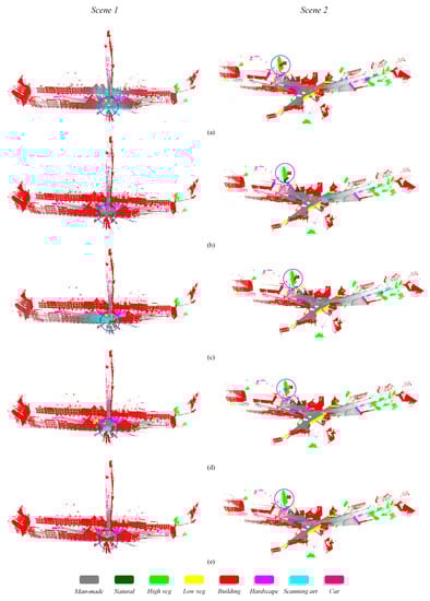
Figure 4.
Classification results of five different approaches on the reduced-8 test set of Semantic3D dataset: (a) PointNet++ (MSG); (b) PointSIFT; (c) PointConv; (d) LSANet; (e) PEMCNet.
4.3. Hyperparameter Analysis
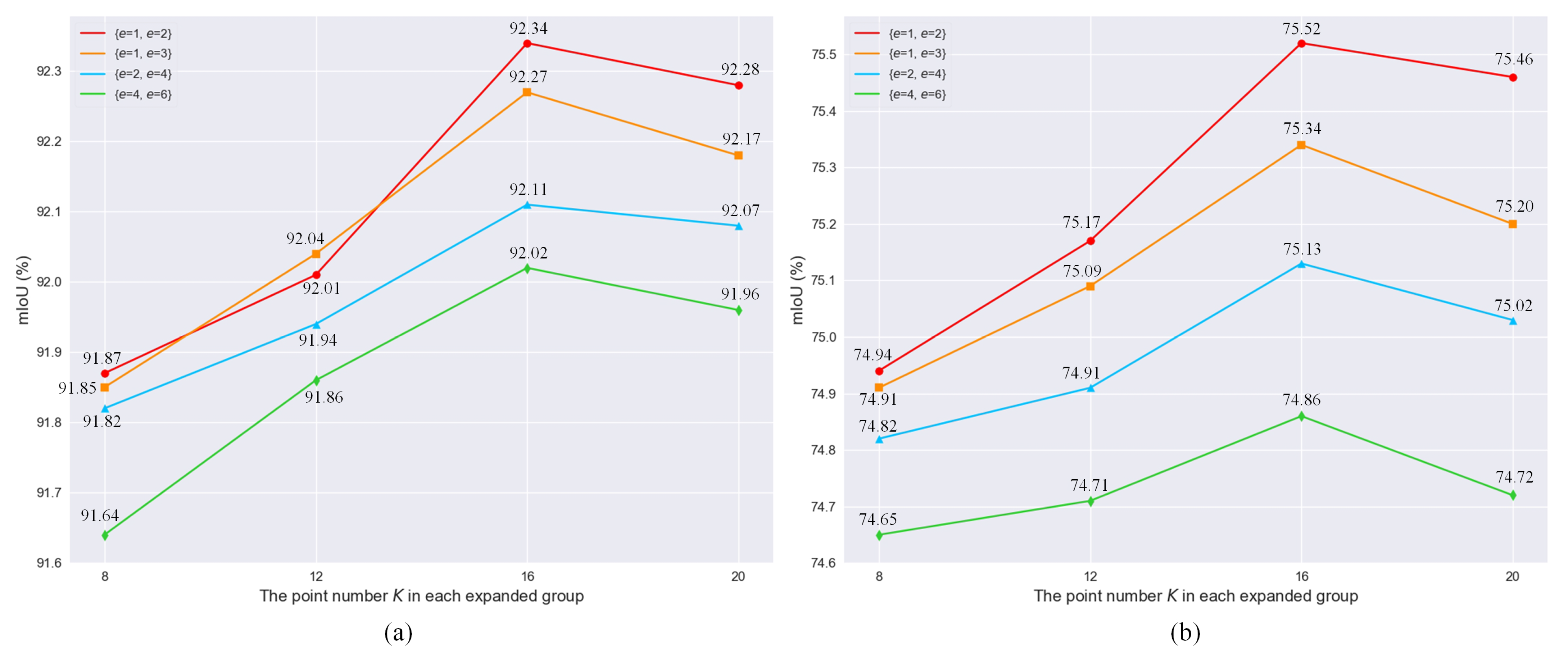
There are two unique hyperparameters, e and K, which play significant roles in the performance of our network. As a lightweight network is preferred, e was fixed in each hierarchy to perform two-scale feature learning. In this study, four different configuration couples of expansion rates were adopted to evaluate the classification performance varying along with different K on both US3D and Semantic3D datasets. As shown in Figure 5a,b, the best-performing configuration for the PEG units on both datasets are the same as , namely the two feature scales in terms of expansion rate e are better to be set as 1 and 2 in each hierarchy. Concerning the number of extracted neighboring points, it can be observed from each subfigure of Figure 5 that, with the same expansion rates, the mIoU achieved on each dataset gradually increases before K arriving at 16. This implies that the classification accuracy can be effectively improved by extracting more point features; however, the mIoU starts to decrease after K = 16. The reduction in classification accuracy on the Semantic3D dataset is more evident as shown in Figure 5b. It means that when K increased to some extent, even though the receptive field of each input point increased and enabled extraction of a larger range of point features, the increase in the receptive field may include other wrong point features, in particular regarding those points of small targets. This would result in the decrease in IoU on those small categories and the overall accuracy in terms of mIoU would also fall as a result.
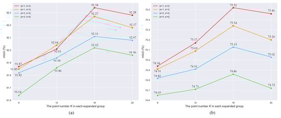
Figure 5.
Classification performance varying with different parameter settings for the PEG unit. Accuracy variations of PEMCNet along with changing K and different expansion rates in terms of mIoU score on US3D dataset (a), PEMCNet on Semantic3D dataset (b).
4.4. Experiments on the UAV-Based Point Cloud Data
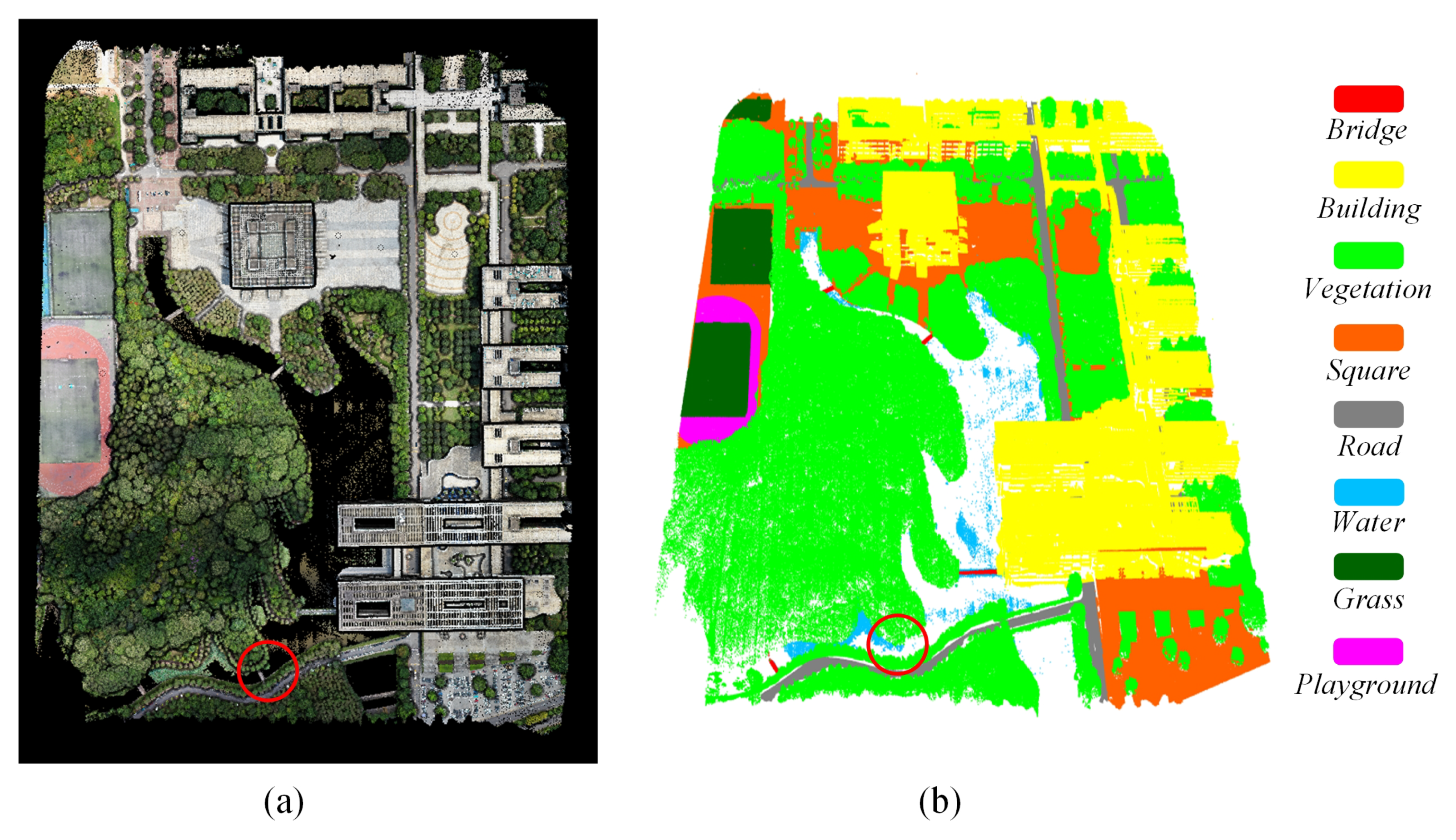
To better validate the robustness of the proposed network, our network was applied to a new collected UAV-based LiDAR point cloud data. This point cloud dataset was acquired at the University Town campus of Guangdong University of Technology (GDUT) on the morning of May 15th, 2021. The point cloud dataset covers an area of about 0.26 km and is denoted as the GDUT Semantic3D dataset (GDUT-S3D). In total 8,318,3070 points were collected by the light airborne LiDAR of RIEGL_VUX-1LR which was equipped on a multicopter. The UAV flew at a height of 105 m along the planned route with the speed set as 6 m/s. The LiDAR sensor in scanning was set at 100 rpm (rounds per minute). The wavelength of the emitted laser is 940 nm. The laser frequency was set as 380 kHz. Its ranging accuracy is 1.5 cm and with 16 bits of high-resolution intensity information per echo. The collected data have a point density of over 100 points/m. The software of LiDAR 360 was used for data inspection. The buildings are clear, while as for the particularity of the structure (open-air design style of buildings) there are cavities that belong to the blind area of airborne scanning. Further, high-resolution RGB images were collected at the same time; therefore, the point cloud data were fused with the RGB image, and a point cloud containing three RGB datapoints, shown in Figure 6a, was generated for study.
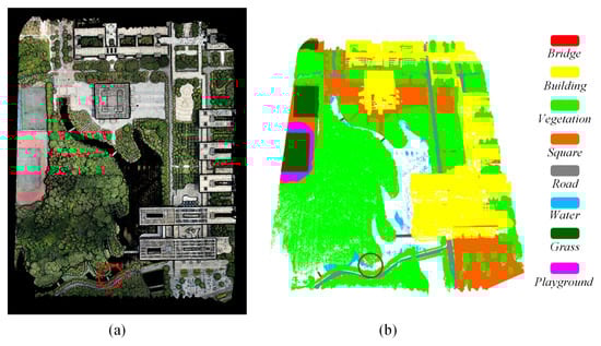
Figure 6.
(a) Point cloud data with RGB information. (b) The classification results of PEMCNet on the test set of the GDUT-S3D dataset.
This point cloud dataset was artificially divided into eight categories, including bridge, building, vegetation, water, road, square, grass, and playground. The point cloud data of the whole scene were divided into nine regions, and 1 million points were taken from each region as training data. Then, the CloudCompare software was used to manually label the points according to the ground truth (high-resolution RGB image). With the labeled data for training. Same parameter settings, such as those used for US3D dataset, were used in this experiment. Finally, the point clouds of the whole scene were tested using the available trained model to predict their labels.
Table 5 and Table 6 show the quantitative classification results of PEMCNet on the test set of the GDUT-S3D dataset. It can be seen that PEMCNet still behaved well on our practical dataset. It achieved satisfactory classification results on those points of large targets, such as building, vegetation, and playground. Figure 6b vividly displayed the classification results. In accordance with the findings from the quantitative classification results, large homogeneous regions such as buildings, vegetation, and playgrounds were predicted as smooth areas with the same labels. As for the ineffectiveness of the 940 nm laser on water, the water in the lake was not well separated, which agrees with its specific classification accuracy of 45.89% (IoU). The small category of the bridge was even worse. A small bridge was missed from the classification results (see the indication of the red circle in Figure 6a,b).
Table 5.
Quantitative classification performance of PEMCNet on the test set of GDUT-S3D dataset.
Table 6.
Classification accuracy of each class of PEMCNet on the test set of GDUT-S3D dataset in terms of IoU (%).
5. Discussion
Effective feature learning plays a vital role in the precise classification of point cloud classification. Regarding the local information learning, it has been revealed that utilizing the points information in a wider neighborhood by expanding the radius of spherical queries or constructing larger K-neighborhood graphs in feature learning helps with the improvement of point cloud classification accuracy [25,29,30]. However, these approaches also consume more time relative to the effort in the searching within an enlarged local searching area. In this study, a point expanded grouping strategy is deployed in the deep neural network for the same sake to extract more neighboring point features in feature learning, but without bringing extra computational burden. The point expanded grouping processing can be regarded as a repetition of K-NN, but being conducted simultaneously. With the distances between the center point and all the rest point samples prepared in advance, PEG needs only one such computation accompanied with sequential storage. Then, given different expansion rates, K neighbor points concerning each corresponding expansion rate can be extracted at the same time, which prompts an efficient learning process and lightweight storage space. The efficiency of our method in terms of both processing time and model size indicated the priority of our method with Table 1, Table 3, and Table 5. This strategy also works similar to the strategy of expanding the radius of spherical queries to include more local points for feature learning [25,29]; therefore, it is reasonable for our method to have merit similar to those approaches. The strategy used here in fact realizes an enlarged conceptive field that enables us to summarize the local information for feature learning. Of more importance, it renders multi-scale context information retrieval in dense point clouds. Moreover, the spatial relationship between those extracted point features is better represented for further learning by taking into consideration both coordinates information and the relative position between points. It can be observed from the experimental results that those especially competitive classification accuracy achieved with our network (see Table 2, Table 4, and Table 6) were corresponding to the class types associated with large homogeneous areas. As seen from the corresponding classification maps, those areas obtained much smoother classification results. Such facts are in accordance with the above analysis. While for the relatively small targets (bridge in GDUT-S3D data) or small heterogeneous areas (Man-made and Natural in Semantic3D data), the accuracies were not promising in Table 4 and Table 6, respectively. Accompanied with the parameter analysis results, Figure 5 shows the most potential classification lies on proper parameter setting. Regarding the remotely sensed point cloud datasets with different characteristics, too large expansion rates cannot lead to promising results. The expansion rate couple is a potential empirical choice that may be effective for more applications.
6. Conclusions
In this paper, we proposed an efficient PEMCNet to aggregate multi-scale local geometric details in feature learning for the classification of large-scale 3D LiDAR point clouds. The multi-scale feature learning for the point cloud is realized by (1) introducing a novel point grouping method—PEG unit to capture multi-scale point features of flexibly varied receptive fields with an expansion rate without introducing more parameters; (2) introducing an ARSE unit to effectively preserve the spatial relationship between each centroid point and its neighboring points. The classification experiments on both US3D and Semantic3D datasets demonstrate the excellent performance of our network. In summary, our method not only achieves promising classification accuracy on both public and newly collected practical datasets but also is efficient in terms of both time and memory. With over 91% of classification accuracy and less than 200 ms of model forward time on all the datasets, our network has demonstrated the potential priority in the classification of especially large homogeneous areas; therefore, our architectures can be conveniently applied in classification tasks of large-scale 3D LiDAR point clouds.
Author Contributions
Conceptualization, G.Z. and W.Z.; methodology, G.Z. and W.Z.; writing—original draft preparation, G.Z. and W.Z.; writing—review and editing, G.Z., Y.P., H.W., Z.W. and L.C.; funding acquisition, G.Z., Y.P., H.W., Z.W. and L.C. All authors have read and agreed to the published version of the manuscript.
Funding
This research was funded in part by the National Natural Science Foundation of China under Grant (61701123, 62173098, 61805048, 51905351), Guangdong Provincial Key Laboratory of Cyber-Physical System under Grant (2020B1212060069), High Resolution Earth Observation Major Project under Grant (83-Y40G33-9001-18/20), Provincial Agricultural Science and Technology Innovation and Extension project of Guangdong Province under Grant (2019KJ147), Opening Foundation of Key Laboratory of Environment Change and Resources Use in Beibu Gulf Ministry of Education (Nanning Normal University) (NNNU-KLOP-K1935, NNNU-KLOPK1936), Science and technology projects of Guangdong Province (2016B010127005) and Science and Technology Planning Project of Shenzhen Municipality of China under Grant (JCYJ20190808113413430).
Conflicts of Interest
The authors declare no conflict of interest.
References
- Wen, C.; Yang, L.; Li, X.; Peng, L.; Chi, T. Directionally constrained fully convolutional neural network for airborne LiDAR point cloud classification. ISPRS J. Photogramm. Remote Sens. 2020, 162, 50–62. [Google Scholar] [CrossRef] [Green Version]
- Liu, W.; Sun, J.; Li, W.; Hu, T.; Wang, P. Deep Learning on Point Clouds and Its Application: A Survey. Sensors 2019, 19, 4188. [Google Scholar] [CrossRef] [Green Version]
- Ioannidou, A.; Chatzilari, E.; Nikolopoulos, S.; Kompatsiaris, I. Deep Learning Advances in Computer Vision with 3D Data: A Survey. ACM Comput. Surv. 2017, 50, 20:1–20:38. [Google Scholar] [CrossRef]
- Qiu, Q.; Sun, N.; Bai, H.; Wang, N.; Fan, Z.; Wang, Y.; Meng, Z.; Li, B.; Cong, Y. Field-Based High-Throughput Phenotyping for Maize Plant Using 3D LiDAR Point Cloud Generated with a “Phenomobile”. Front. Plant Sci. 2019, 10, 554. [Google Scholar] [CrossRef] [PubMed] [Green Version]
- Yang, B.; Huang, R.; Li, J.; Tian, M.; Dai, W.; Zhong, R. Automated Reconstruction of Building LoDs from Airborne LiDAR Point Clouds Using an Improved Morphological Scale Space. Remote Sens. 2017, 9, 14. [Google Scholar] [CrossRef] [Green Version]
- Ali, W.; Abdelkarim, S.; Zidan, M.; Zahran, M.; Sallab, A.E. YOLO3D: End-to-End Real-time 3D Oriented Object Bounding Box Detection from LiDAR Point Cloud. In Proceedings of the 2018 European Conference on Computer Vision (ECCV), Munich, Germany, 8–14 September 2018; pp. 1–12. [Google Scholar]
- Neuville, R.; Bates, J.; Jonard, F. Estimating Forest Structure from UAV-Mounted LiDAR Point Cloud Using Machine Learning. Remote Sens. 2021, 13, 352. [Google Scholar] [CrossRef]
- Zhang, W.; Qiu, W.; Song, D.; Xie, B. Automatic Tunnel Steel Arches Extraction Algorithm Based on 3D LiDAR Point Cloud. Sensors 2019, 19, 3972. [Google Scholar] [CrossRef] [PubMed] [Green Version]
- Elbaz, G.; Avraham, T.; Fischer, A. 3D Point Cloud Registration for Localization Using a Deep Neural Network Auto-Encoder. In Proceedings of the IEEE Conference on Computer Vision and Pattern Recognition, Honolulu, HI, USA, 21–26 July 2017; pp. 4631–4640. [Google Scholar]
- Maturana, D.; Scherer, S. 3D Convolutional Neural Networks for landing zone detection from LiDAR. In Proceedings of the IEEE International Conference on Robotics and Automation (ICRA 2015), Seattle, WA, USA, 26–30 May 2015; pp. 3471–3478. [Google Scholar]
- Tonina, D.; McKean, J.A.; Benjankar, R.M.; Wright, C.W.; Goode, J.R.; Chen, Q.; Reeder, W.J.; Carmichael, R.A.; Edmondson, M.R. Mapping river bathymetries: Evaluating topobathymetric LiDAR survey. Earth Surf. Process. Landf. 2019, 44, 507–520. [Google Scholar] [CrossRef]
- Widyaningrum, E.; Gorte, B.G.H. Comprehensive comparison of two image-based point clouds from aerial photos with airborne LiDAR for large-scale mapping. Int. Arch. Photogramm. Remote Sens. Spat. Inf. Sci. 2017, 42, 557–565. [Google Scholar] [CrossRef] [Green Version]
- Chen, S.; Liu, B.; Feng, C.; Vallespi-Gonzalez, C.; Wellington, C. 3D Point Cloud Processing and Learning for Autonomous Driving. arXiv 2020, arXiv:2003.00601. [Google Scholar]
- Wang, M.; Dong, H.; Zhang, W.; Chen, C.; Lu, Y.; Li, H. An End-to-end Auto-driving Method Based on 3D LiDAR. J. Phys. Conf. Ser. 2019, 1288, 012061. [Google Scholar] [CrossRef]
- Chen, X.; Ma, H.; Wan, J.; Li, B.; Xia, T. Multi-view 3D Object Detection Network for Autonomous Driving. In Proceedings of the 2017 IEEE Conference on Computer Vision and Pattern Recognition, CVPR 2017, Honolulu, HI, USA, 21–26 July 2017; pp. 6526–6534. [Google Scholar]
- Bello, S.A.; Yu, S.; Wang, C.; Adam, J.M.; Li, J. Review: Deep Learning on 3D Point Clouds. Remote Sens. 2020, 12, 1729. [Google Scholar] [CrossRef]
- Ahmed, E.; Saint, A.; Shabayek, A.E.R.; Cherenkova, K.; Das, R.; Gusev, G.; Aouada, D.; Ottersten, B. Deep learning advances on different 3D data representations: A survey. arXiv 2018, arXiv:1808.01462. [Google Scholar]
- Hana, X.-F.; Jin, J.S.; Xie, J.; Wang, M.-J.; Jiang, W. A Comprehensive Review of 3D Point Cloud Descriptors. arXiv 2018, arXiv:1802.02297. [Google Scholar]
- Guo, Y.; Wang, H.; Hu, Q.; Liu, H.; Liu, L.; Bennamoun, M. Deep Learning for 3D Point Clouds: A Survey. arXiv 2019, arXiv:1912.12033. [Google Scholar] [CrossRef]
- Grilli, E.; Menna, F.; Remondino, F. A review of point clouds segmentation and classification algorithms. ISPRS Int. Arch. Photogramm. Remote. Sens. Spat. Inf. Sci. 2017, 42, 339–344. [Google Scholar] [CrossRef] [Green Version]
- Qi, C.R.; Su, H.; Nießner, M.; Dai, A.; Yan, M.; Guibas, L.J. Volumetric and Multi-view CNNs for Object Classification on 3D Data. In Proceedings of the 2016 IEEE Conference on Computer Vision and Pattern Recognition (CVPR 2016), Las Vegas, NV, USA, 27–30 June 2016; pp. 5648–5656. [Google Scholar]
- Wang, C.; Cheng, M.; Sohel, F.; Bennamoun, M.; Li, J. NormalNet: A voxel-based CNN for 3D object classification and retrieval. Neurocomputing 2019, 323, 139–147. [Google Scholar] [CrossRef]
- Su, H.; Maji, S.; Kalogerakis, E.; Learned-Miller, E.G. Multi-view Convolutional Neural Networks for 3D Shape Recognition. In Proceedings of the 2015 IEEE International Conference on Computer Vision (ICCV 2015), Santiago, Chile, 7–13 December 2015; pp. 945–953. [Google Scholar]
- Charles, R.Q.; Su, H.; Kaichun, M.; Guibas, L.J. PointNet: Deep Learning on Point Sets for 3D Classification and Segmentation. In Proceedings of the 2017 IEEE Conference on Computer Vision and Pattern Recognition (CVPR), Honolulu, HI, USA, 21–26 July 2017; pp. 77–85. [Google Scholar]
- Qi, C.R.; Yi, L.; Su, H.; Guibas, L.J. PointNet++: Deep Hierarchical Feature Learning on Point Sets in a Metric Space. In Advances in Neural Information Processing Systems 30; Guyon, I., Luxburg, U.V., Bengio, S., Wallach, H., Fergus, R., Vishwanathan, S., Garnett, R., Eds.; Curran Associates, Inc.: Red Hook, NY, USA, 2017; pp. 5099–5108. [Google Scholar]
- Jiang, M.; Wu, Y.; Zhao, T.; Zhao, Z.; Lu, C. PointSIFT: A SIFT-like Network Module for 3D Point Cloud Semantic Segmentation. arXiv 2018, arXiv:1807.00652. [Google Scholar]
- Lowe, D.G. Distinctive image features from scale-invariant keypoints. Int. J. Comput. Vis. 2004, 60, 91–110. [Google Scholar] [CrossRef]
- Wu, W.; Qi, Z.; Fuxin, L. Pointconv: Deep convolutional networks on 3d point clouds. In Proceedings of the IEEE Conference on Computer Vision and Pattern Recognition (CVPR), Long Beach, CA, USA, 16–20 June 2019; pp. 9621–9630. [Google Scholar]
- Chen, L.; Li, X.; Fan, D.; Wang, K.; Lu, S.; Cheng, M. LSANet: Feature learning on point sets by local spatial aware layer. arXiv 2019, arXiv:1905.05442. [Google Scholar]
- Hu, Q.; Yang, B.; Xie, L.; Rosa, S.; Guo, Y.; Wang, Z.; Trigoni, N.; Markham, A. RandLA-Net: Efficient semantic segmentation of large-scale point clouds. In Proceedings of the Computer Vision and Pattern Recognition (CVPR), Long Beach, CA, USA, 16–20 June 2019; pp. 11108–11117. [Google Scholar]
- Sutskever, I.; Vinyals, O.; Le, Q.V. Sequence to sequence learning with neural networks. In Advances in Neural Information Processing Systems; Neural Information Processing Systems Foundation, Inc.: South Lake Tahoe, NV, USA, 2014; pp. 3104–3112. [Google Scholar]
- Wang, X.; Jin, Y.; Cen, Y.; Wang, T.; Li, Y. Attention models for point clouds in deep learning: A survey. arXiv 2021, arXiv:2102.10788. [Google Scholar]
- Guo, M.; Cai, J.; Liu, Z.; Mu, T.; Martin, R.R.; Hu, S. PCT: Point Cloud Transformer. arXiv 2020, arXiv:2012.09688. [Google Scholar]
- Wang, L.; Huang, Y.; Hou, Y.; Zhang, S.; Shan, J. Graph Attention Convolution for Point Cloud Semantic Segmentation. In Proceedings of the IEEE Conference on Computer Vision and Pattern Recognition (CVPR), Long Beach, CA, USA, 16–20 June 2019; pp. 10296–10305. [Google Scholar]
- Vaswani, A.; Shazeer, N.; Parmar, N.; Uszkoreit, J.; Jones, L.; Gomez, A.N.; Kaiser, Ł.; Polosukhin, I. Attention is all you need. In Advances in Neural Information Processing Systems; MIT Press: Long Beach, CA, USA, 2017; pp. 5998–6008. [Google Scholar]
- Gardner, M.; Dorling, S. Artificial neural networks (the multilayer perceptron)—A review of applications in the atmospheric sciences. Atmos. Environ. 1998, 32, 2627–2636. [Google Scholar] [CrossRef]
- Bosch, M.; Foster, K.; Christie, G.; Wang, S.; Hager, G.D.; Brown, M. Semantic Stereo for Incidental Satellite Images. In Proceedings of the 2019 IEEE Winter Conference on Applications of Computer Vision, Waikoloa Village, HI, USA, 7–11 January 2019; pp. 1524–1532. [Google Scholar]
- Hackel, T.; Savinov, N.; Ladicky, L.; Wegner, J.D.; Schindler, K.; Pollefeys, M. SEMANTIC3D.NET: A new large-scale point cloud classification benchmark. ISPRS Ann. Photogramm. Remote Sens. Spat. Inf. Sci. 2017, IV-1-W1, 91–98. [Google Scholar] [CrossRef] [Green Version]
Publisher’s Note: MDPI stays neutral with regard to jurisdictional claims in published maps and institutional affiliations. |
© 2021 by the authors. Licensee MDPI, Basel, Switzerland. This article is an open access article distributed under the terms and conditions of the Creative Commons Attribution (CC BY) license (https://creativecommons.org/licenses/by/4.0/).