Abstract
We aim to develop a comprehensive tunnel lining detection method and clustering technique for semi-automatic rebar identification in order to investigate the ten tunnels along the South-link Line Railway of Taiwan (SLRT). We used the Ground Penetrating Radar (GPR) instrument with a 1000 MHz antenna frequency, which was placed on a versatile antenna holder that is flexible to the tunnel’s condition. We called it a Vehicle-mounted Ground Penetrating Radar (VMGPR) system. We detected the tunnel lining boundary according to the Fresnel Reflection Coefficient (FRC) in both A-scan and B-scan data, then estimated the thinning lining of the tunnels. By applying the Hilbert Transform (HT), we extracted the envelope to see the overview of the energy distribution in our data. Once we obtained the filtered radargram, we used it to estimate the Two-dimensional Forward Modeling (TDFM) simulation parameters. Specifically, we produced the TDFM model with different random noise (0–30%) for the rebar model. The rebar model and the field data were identified with the Hierarchical Agglomerative Clustering (HAC) in machine learning and evaluated using the Silhouette Index (SI). Taken together, these results suggest three boundaries of the tunnel lining i.e., the air–second lining boundary, the second–first lining boundary, and the first–wall rock boundary. Among the tunnels that we scanned, the Fangye 1 tunnel is the only one in category B, with the highest percentage of the thinning lining, i.e., 13.39%, whereas the other tunnels are in category A, with a percentage of the thinning lining of 0–1.71%. Based on the clustered radargram, the TDFM model for rebar identification is consistent with the field data, where k = 2 is the best choice to represent our data set. It is interesting to observe in the clustered radargram that the TDFM model can mimic the field data. The most striking result is that the TDFM model with 30% random noise seems to describe our data well, where the rebar response is rough due to the high noise level on the radargram.
1. Introduction
The South-link Line Railway of Taiwan (SLRT) serves as an important means of transportation that passes through the southern Central Mountain Range of Taiwan, and has been operating for approximately 20 years, since 1991. It consists of 36 mountain tunnels with a total length of 38.9 km, embankments and bridges with a total length of 8.8 km, and slope-land sections that extend from the Pingtung County to the Taitung County (0k+000 to 98k+145) in southern Taiwan [1,2]. In general, the geological condition along the SLRT belongs to the alluvium and weathering rock strata, where various landforms and geological zones exist, such as strike-slip fault, steep slope-land, anticline, and syncline, making this route a relatively high risk to landslide and debris flow hazards. As reported by the Taiwan Railway Administration, in the past decade, several shallow landslides, rockfall, and debris flow triggered by the typhoon HAIMA, typhoon HAITANG, 0614 Rainfall, and 0831 Rainfall events occurred. Thus, a regular inspection is needed, especially for the lining condition of the tunnels in this route [1,3,4,5]. As one of the essential parts of the supporting structure, the tunnel lining is useful for providing the correct shape to the tunnel, strengthening the structure, counteracting the pressure of the wall rock, and preventing the tunnel from collapsing. If the thickness of the lining is thinner than the original design, the potential of collapsing will be higher, and major structural damage will occur [2,6,7]. Many researchers have turned their interest to using a non-destructive geophysical method, i.e., the GPR method, because it provides an efficient way to investigate and analyze the sublayer for any target area without causing any damage. There are several studies reported that apply GPR for inspecting the tunnel lining, such as Parkinson and Ékes [8], who used GPR to map the tunnel lining and locate the concrete deterioration in a water supply tunnel, and their processed data provided a wealth of information on the condition of the tunnel lining. Li, Li [9] applied GPR for the second lining recognition and thickness evaluation in the tunnel by tracing the phase and amplitude of the reflective wave. Xiang, Zhou [10] integrated the GPR and Finite-Difference Time-Domain (FDTD) methods based on the basic information regarding the design of the tunnel structure, where the results are used to interpret the field data, such as the thickness of the second lining and the possible damage zones. Later, in order to improve the detection speed, Zan, Li [11] connected the GPR antenna to the body of the train and scanned the tunnel when the train traveled through it. However, there are several important factors to consider in order to use this system, such as the fact that the scanning rate of the GPR instrument should be high enough to keep up with the train speed, and the distance between the antenna and catenary should be fixed to avoid the collisions, so the initial condition of the tunnel should be known in advance, e.g., the existence of the messenger wire, the catenary, and the surface of the tunnel itself. Alani and Tosti [12] adapted the GPR with different frequency antennas systems (900 MHz and 2 GHz) to study the structural detailing of the major tunnel located underneath. There was a higher resolution with the 2 GHz antenna used to achieve the higher clarity, in comparison to the 900 MHz antenna, but less of a skin depth. However, this study confirmed that both showed the same features inside the lining, and both can be considered as verified. Lately, due to the rapid development of technology, researchers have been intrigued to use machine learning to process the radargram (GPR data). For example, Dinh, Zayed [13] described the clustering-based threshold model based on the GPR data to evaluate the condition of the concrete bridge decks, and continued his work in 2018 to develop the automatic algorithm for the localization and detection of rebar in the same target [14]. Dou, Wei [15] utilized the real-time hyperbola recognition and fitting in GPR data by a column-connection clustering (C3) algorithm, and Liang, Xing [16] then adapted the same algorithm for plant root detection based on the GPR data. Kilic and Eren [17] applied the Neural Network (NN) algorithm for the GPR data to inspect the voids and karst conduits in hydro-electric power station tunnels. Ozkaya, Melgani [18] proposed a Convolutional Support Vector Machine (CSVM) network to analyze the GPR data, which has a similar architecture to a Convolutional Neural Network (CNN). In the same year, Jin and Duan [19] identified a pipeline based on the GPR data with the wavelet scattering network-based machine learning, and a recent study comes from Cui, Quan [20], where they studied the GPR-based automatic identification of root zones using HDBSCAN, or the Hierarchical Density-based Spatial Clustering of Application with Noise.
Previous work has been limited to the fixed GPR system, where the initial condition of the tunnel should be known in advance. In fact, not every tunnel has detailed information about its recent condition. We have undergone a rethinking of this problem by developing a Vehicle-Mounted Ground Penetrating Radar (henceforth named VMGPR) system by combining the GPR instrument with a versatile antenna holder device, inspired by the truck crane, that can be adjusted in every tunnel condition [21]. Our method is a clear improvement and has many beneficial and effective applications on the field. We applied VMGPR due to the rapid result of this method, considered the study area, which is only able to be conducted during midnight in order to avoid the railway’s operating time so that the normal commuting trains would not pass through and get in the way of the scanning process. The main objectives of this paper are to detect the lining and to identify the reinforcement bar (rebar) of the mountain tunnel. Here, we used an automatic continuous picking phase based on the Fresnel reflection coefficient to detect the lining, while implementing the clustering methods in machine learning to identify the rebar. Even though various machine learning approaches have been proposed for GPR data, very few studies reported the use of Hierarchical Agglomerative Clustering (HAC), especially for tunnel inspection. This technique uses the bottom-up algorithm, where each data observation starts in its own cluster (leaves), and then successively merges pairs of clusters until all clusters have been merged into one big cluster that contains all data [22]. Furthermore, we simulated the Two-Dimensional Forward Modeling (TDFM) for each case to validate and interpret our results. The attempt of our methods may show an alternative way to inspect and evaluate the mountain tunnel with a comprehensive result.
2. Materials and Methods
2.1. The Site Description and the GPR Measurements
There are two types of tunnels in the SLRT route: six tunnels between the Central Signal station to the Guzhuang station are Double-Rail Tunnels (DRT), whereas the rest of them were built with Single-Rail Tunnels (SRT). In this study, we focused on the ten single-rail tunnels along the Fangshan Township to the Shihzih Township i.e., Fangdian 1 (FD1), Fangdian 2 (FD2), Fangshan 1 (FS1), Fangshan 2 (FS2), Fangshan 3 (FS3), Fangshan 4 (FS4), Fangshan 5 (FS5), Fangye 1 (FY1), Fangye 2 (FY2), and Fangye 3 (FY3), where the length of the tunnels are 40 m, 85 m, 300 m, 585 m, 688 m, 156 m, 205 m, 1809 m, 722 m, and 1360 m, respectively (Figure 1).
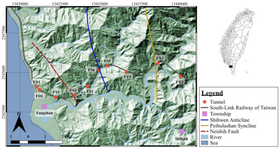
Figure 1.
The geographic map along the South-link Line Railway of Taiwan. The red pentagonal shows the tunnel along this line, and the red-dashed line, blue line, and orange line are the Neishih Fault, the Shihwen Anticline, and the Peihulushan Syncline, respectively.
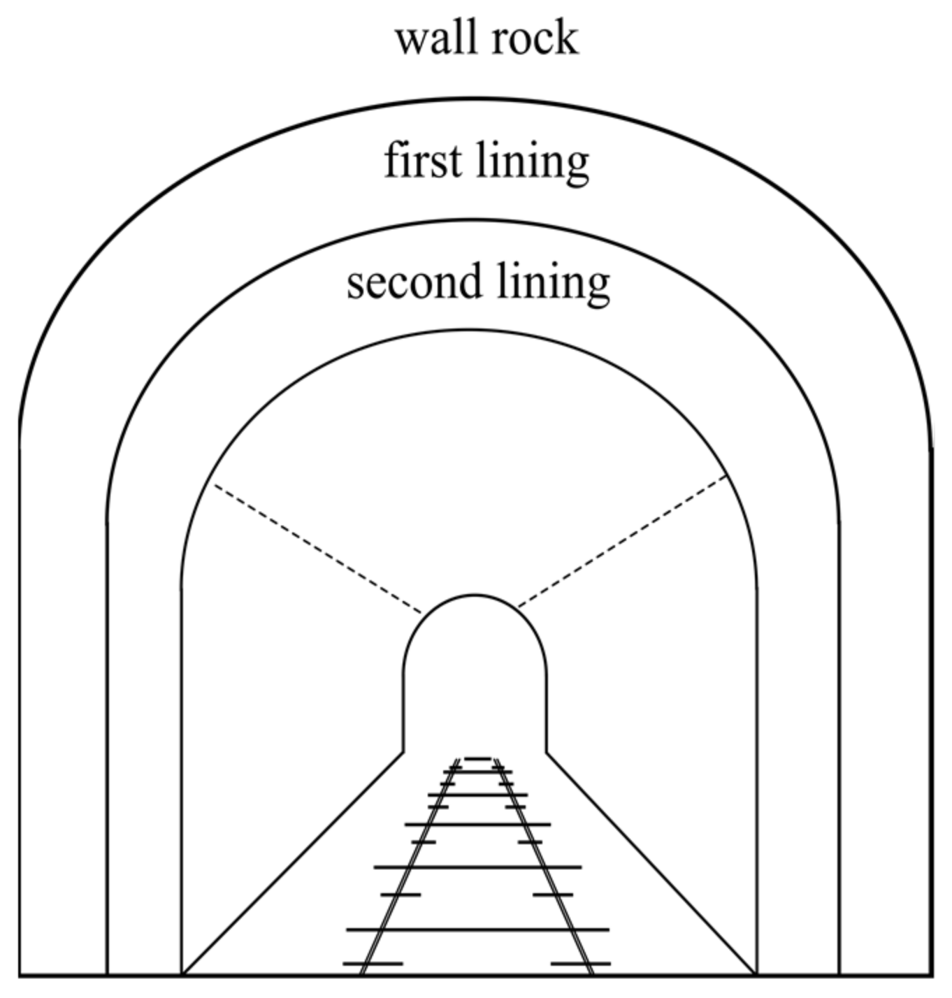
The tunnel consists of different layers, such as the second lining and the first lining, while the wall rock is the surrounding rocks that cover the tunnel, as shown in Figure 2. The SLRT route also crossed the Neishih Fault nearby the Fangdian 2 tunnel, the Shihwen Anticline nearby the Fangshan 4 tunnel, and the Peihulushan Syncline nearby the Fangye 2 tunnel. Furthermore, the Chaochou Fault is found on the southern side of the SLRT, which separates the Pingtung Plain from the Central Range. Due to the presence of a thick quaternary strata section in the basin to the west and the Miocene-age rocks in the mountains on the east, it is demonstrated that the fault has a significant component of vertical slip, up on the east side [23,24]. These various geological conditions make this area a vulnerable zone for geological hazards. We used the GPR instrument from Sensor and Software, Inc. with a 1000 MHz antenna frequency, which was placed on a versatile antenna holder that is flexible to the tunnel’s condition. Later, we called it a VMGPR. The VMGPR was set up on a small train with the antenna facing the surface of the lining, and it traveled along the railroad tracks inside the tunnel in free-run mode and set to a reflection survey type with a constant and low speed of around 20 km/h in order to maintain the quality of the data. The scanned result showed real-time raw data on the Digital Video Logger (DVL), which then stored them into the external memory card. Furthermore, we processed and analyzed the GPR data with several steps, as shown in Figure 3.
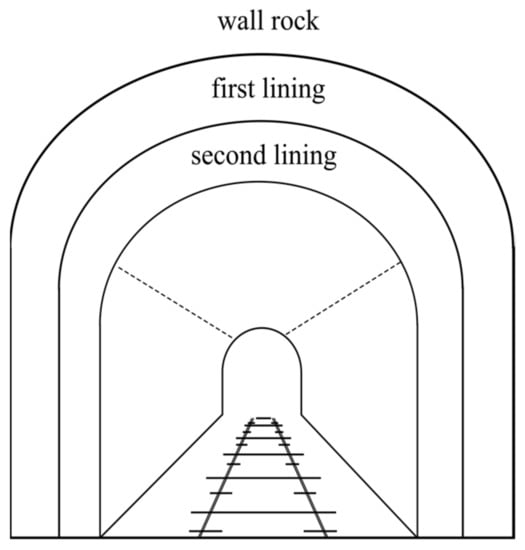
Figure 2.
The principle layers of the tunnel. It consists of the second lining, the first lining, and the wall rock from inside to outside.
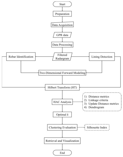
Figure 3.
The workflow of this study.
2.2. The Processing of GPR Data
The GPR raw data require filtering and editing steps in order to make the radargram viewable and interpretable. In this study, we applied four steps, such as dewow data, time-zero correction, background removal, and gain, by using Reflexw software [25]. Firstly, we applied dewow data, which aim to eliminate the possible low-frequency noise (wow), or DC-bias data, which arise either from the close juxtaposition of the antennas (receiver–transmitter) or the inductive phenomena, which can generate a distortion of the mean of A-scan towards values of amplitude that are far from zero; this noise should be removed before applying other filters. We processed the data by a simple filter that acts within the time domain, called subtract-mean (works on each trace). A running mean that is subtracted from the central point is computed for each value of each trace, with the time range value set to one principal period using an average subtraction algorithm, such as [25,26,27]:
where D(n) is the amplitude of the nth processed trace, Dr(n) is the amplitude of the raw trace, and D(k) is the average amplitudes of the traces. Secondly, the time delay of the first arrival was corrected with the time-zero correction. This possibly occurred because of several reasons, such as the temperature difference between the GPR instrument and the surrounding environment during the data acquisition, and/or unstable distance between the antenna and the ground [27,28,29]. Thirdly, a spatial filter for B-scan (filter for some trace data) is applied, i.e., background removal. In this case, the radargram is often adulterated by clutter that mostly appears as periodical ringing, where this phenomenon appears as closely horizontal events or flat-lying reflectors [25,26,27,30,31,32]. This procedure to remove this feature is shown as followed:
where D(n) and Dr(n) are the processed and raw nth signal traces, and k is the number of the trace within the selected set of A-scans. Fourthly, the gain is applied to compensate for the signal attenuation or to strengthen the radargram’s signal. When the waves are propagating to the ground, the signal suffers from an attenuation. The signal from the greater depth is minimal compared to the upper part, and any target or structure in the lower part of the radargram will either appear as imperceptible or just faintly along the lines, bringing out a very unsatisfactory image of radargram. Here, we used the time-varying gain, which can represent a useful mean for illuminating and interpreting deeper information in the inner lining of the tunnel [25,26,27,32]. Generally, the time-varying gain function can be explained as follows:
where D(n) is the nth sample of the trace in the time domain, and k is the gaining function of the n sample. These steps will produce the filtered radargram, which is then used to determine the layer and thickness of tunnel lining.
2.3. The Tunnel Lining Detection Method
The tunnel lining can be identified using the Fresnel Reflection Coefficient (FRC). This describes the reflection of the electromagnetic wave (EM wave) at the point when it arrives at the interface between two media with different electromagnetic properties. It is expressed in Equation (4) as
where γ is the reflection coefficient, α1 is the incident angle, and α2 is the refraction angle. η1 and η1 are the wave impedance for two media, expressed as
where ε1 and ε2 are the relative permittivity of the medium 1 and medium 2. μ1 and μ1 are the relative magnetic permeability, where, in concrete, μ = 1. Due to the small distance between the transmitter antenna and receiver antenna of the GPR system, the transmission direction of electromagnetic field is vertical to the incident plane. If we consider all of these factors, the FRC in the two media is expressed as
Equation (6) is an important form for the lining identification. Different media will have different ε, so that, when the wave propagates and hits the boundary between two media, the reflection coefficient will increase or decrease and the amplitude of reflective wave will also change. If ε1 > ε2, the FRC is positive, where the phase of the reflective wave is the same as the incident, and vice versa, If ε1 < ε2, the FRC is negative, where the phase of reflective wave is the reverse of the incident. Further, these assumptions are used to find the lining of the tunnel [9,26,33,34,35,36,37].
2.3.1. The Lining Detection in A-Scan
A-scan is the basic measurement for the time domain. It is a single waveform recorded by GPR. When the waves’ amplitude abruptly increases or decreases, it may be a sign that the wave is hitting the interface between two media. There are two conditions for when the wave is traveling through different media behind the surface of the tunnel:
- The Boundary Between the Air Layer to the Second Lining
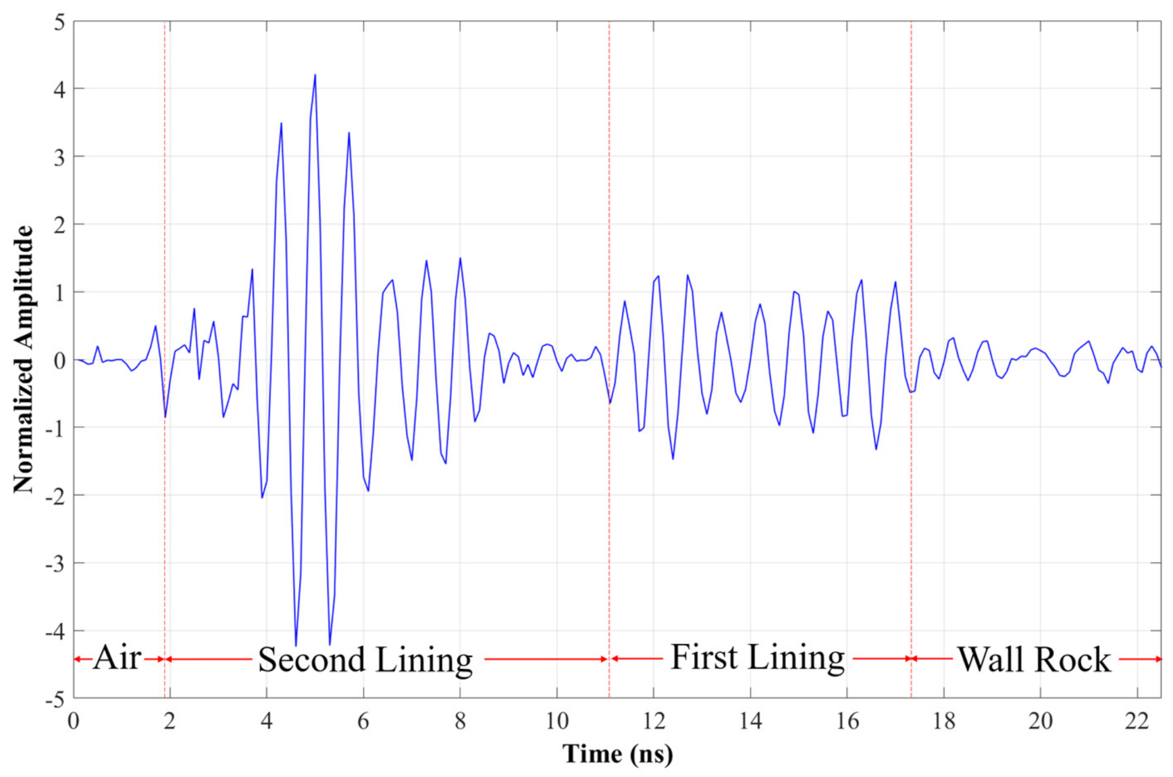
The reflective wave barely attenuates when the electromagnetic waves are transmitted in the air. If the amplitude is abruptly increased or decreased, the wave may arrive in the other medium. Based on the FRC (Equation (6)), if the wave travels from the air with a relative permittivity of 1 to the second lining, which consists of concrete with a relative permittivity in the range of 4–10 [26,32,38], the FRC is negative, which means that the phase of the reflective wave is the reverse of the incident. Hence, we picked it as the boundary between the air layer and the second lining. Figure 4 shows the waveform of the GPR data in the tunnel, where the boundary of these layers is marked as at around 2 ns.
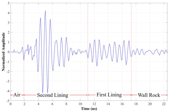
Figure 4.
The filtered A-scan. It shows the boundary of each lining, which is marked with red-dashed line, such as the air layer, the second lining, the first lining, and the wall rock.
- The Boundary Between the Second Lining to the First Lining
Generally, the relative permittivity of the first lining (ε3) is higher than the second lining (ε2). This can occur due to the existence of moisture inside the first lining, which is directly in contact with the wall rock that contains water in its pores. Due to the fact that ε2 < ε3, the FRC is negative, i.e., the phase of the reflective wave is reverse to the incident. Based on this information, we picked the boundary of these layers as at around 11 ns. We did not pick the highest amplitude at around 4–6 ns because it is the response of the rebars inside the second lining (Figure 4).
2.3.2. The Lining Detection in B-Scan
B-scan is 2D data that are formed by gathering a set of A-scan data along the x-axis or in a particular direction (e.g., Figure 5).
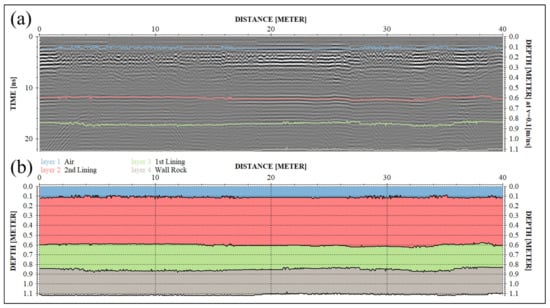
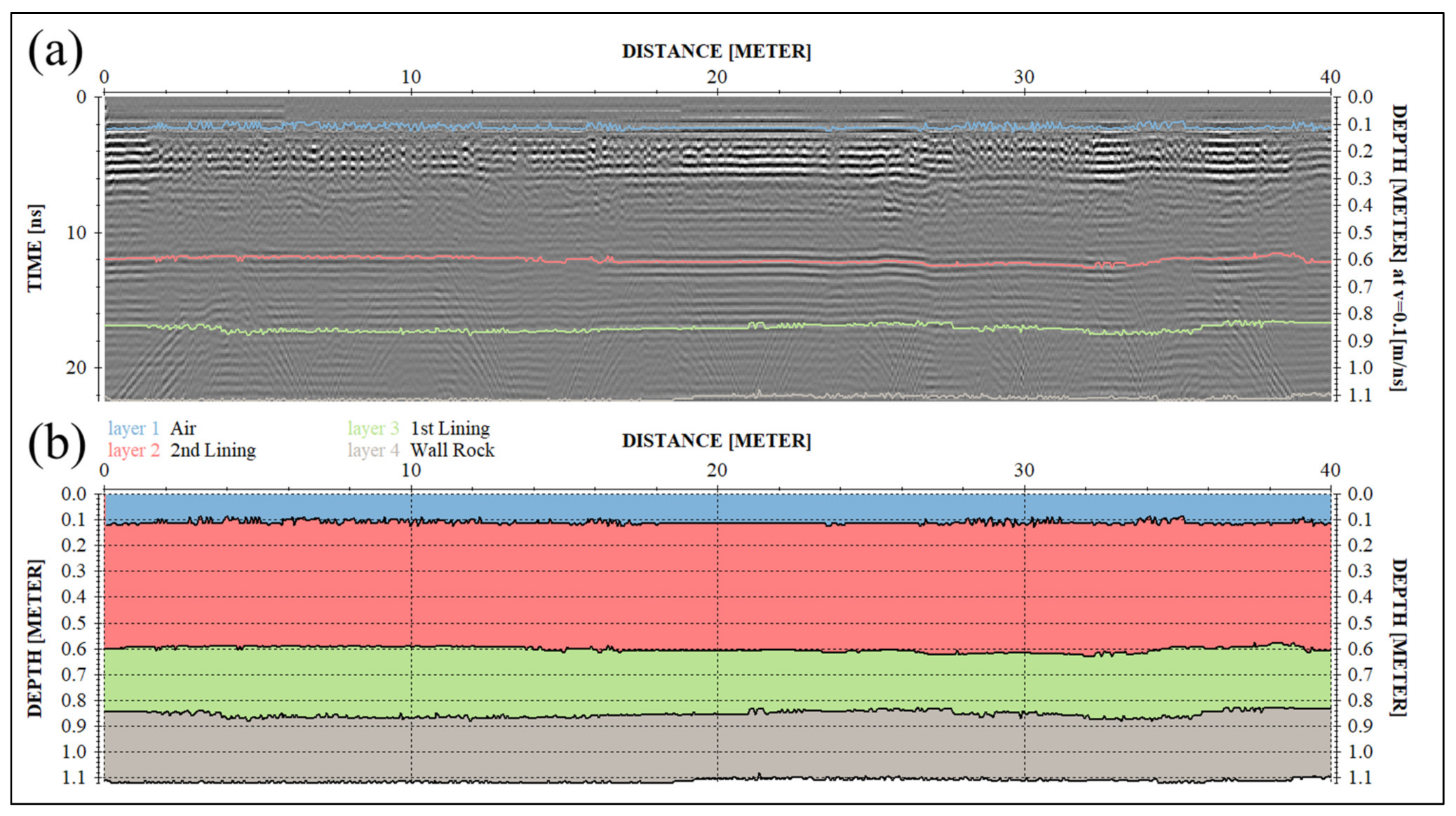
Figure 5.
(a) The filtered radargram with grayscale palette from the GPR scanning in the tunnel Fangdian I, with total distance of 40 m (12k+763.7 to 12k+804.1); (b) the layer interpretation in the B-scan. The blue color is the air layer, the peach color is the second lining, the green color is the first lining, and the brown color is the wall rock.
In 2D radargram, the time axis is usually pointed downwards and is related to the depth of the radargram, whereas the horizontal axis is the distance or surface position. The boundaries of each layer in B-scan are picked automatically and continuously based on A-scan data, and the amplitude value is represented in a grayscale color bar, where the darker color is the negative amplitude and the lighter color is the positive amplitude. Referring to the lining detection with A-scan, the phase and amplitude of reflective waves are the pivotal benchmarks for detecting those boundaries. Hence, the strong amplitude with darker color is picked as the interface of each layer.
Once the boundary of each layer is determined, the thickness (d) of the lining can be estimated. Considering that the transmission direction of EM field is vertical to the incident plane, we can use Equation (7) [33,39]:
where v is the EM wave velocity (m/ns), and t is the two-way travel time (ns).
2.4. The Semi-Automatic Rebar Identification
The rebar or reinforcement bar is a rod that provides reinforcement in concrete structures. It can be placed flat or stand straight in the concrete, and can also be in the form of mesh. Generally, the rebar is easy to find in the filtered radargram, where the numerous small hyperbolic patterns almost connected to each other are indicators of its presence. However, this step is known to be the most labor-intensive and time consuming [14], especially if the scanning line is long, as, in this study, we scanned 10 tunnels with a total length of 5950 m at a time. In this situation, it may take several working days or even weeks for the analyst to complete the rebar-picking task only. For this reason, we applied the clustering technique in machine learning to carry out the automatic rebar identification from the filtered radargram i.e., Hierarchical Agglomerative Clustering (HAC) (see the workflow of this study in Figure 3). The HAC presents several advantages compared to other clustering methods. Firstly, in terms of flexibility, this method is easy to implement and applicable to any attribute type of data, e.g., numerical or text. Secondly, it produces a dendrogram, which is a graphical representation that records the sequences of merges or splits between clusters, and so can produce an ordering of the objects, which is more informative than a single partition because it provides more insight or a bigger picture about the relationship between objects and clusters. Thirdly, there is no requirement to set the number of clusters a priori, unlike most flat clustering methods, i.e., k-means. Fourthly, smaller clusters will be generated, which may discover similarities in data. Despite number of advantages of the HAC method, it also has some disadvantages. Firstly, sometimes it is difficult to identify the optimal number of clusters by the dendrogram; however, this problem can be solved by calculating the Silhouette Index (SI) (more details in Section 2.4.2). Secondly, it is irrevocable, thus, when an agglomerative algorithm has joined two clusters, they cannot subsequently be separated. In this case, the initial seeds should be chosen carefully. Thirdly, it involves many arbitrary decisions, e.g., distance metric and linkage criteria, so performing multiple experiments is recommended in order to obtain the actual results’ veracity, where the SI can be used to evaluate the result. Notwithstanding the advantages and disadvantages, this method can be used to solve multiple types of problems [22,40,41].
2.4.1. The Hilbert Transform (HT)
Before the clustering process, we implemented the Hilbert Transform (HT), which is a time-domain transformation that shifts the phase of a signal by 90 degrees. This is required to be carried out in order to obtain clustering result without being influenced by the phase differences in the same layer. Commonly, the HT is used in post-stack seismic analysis or GPR analysis to generate the analytical signal, from which, we can compute the standard complex trace attribute, such as the pulse envelope or instantaneous amplitude, instantaneous phase, and instantaneous frequency.
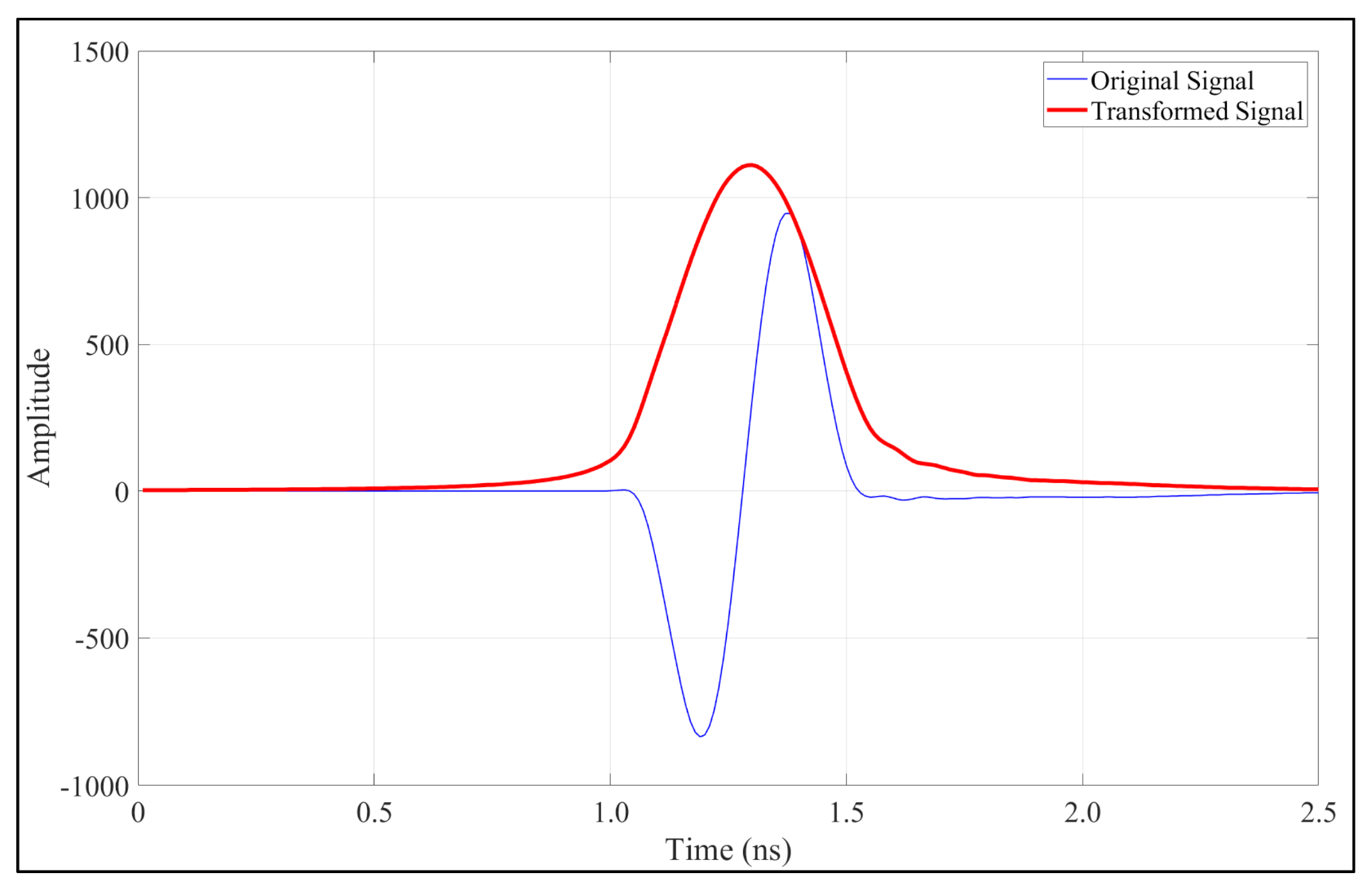
In this study, we used the HT to extract the envelope or instantaneous amplitude that formed from a pair of traces that uniquely bracket the extremes of an oscillatory signal. Specifically, the envelope is related to the reflectivity strength of the signal, which is commensurable to the square root of the signal complete energy at a moment in time (Figure 6). Thus, a strong amplitude may be an indication of the significant changes in structure or material in subsurface; in theory, the analytic signal through its module |h(t)| determines the pulse A(t) envelope [25,42,43], expressed as
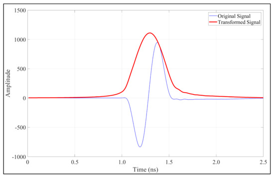
Figure 6.
The blue line is the original signal before HT, and bold red line is the transformed signal by using the HT to extract the envelope or instantaneous amplitude.
2.4.2. The Application of the Hierarchical Agglomerative Clustering (HAC)
After the result from the HT is obtained, we transformed the data into the required format for the clustering process. In this study, we applied the HAC to interpret our data sets. This method is an unsupervised clustering technique that uses bottom-up approaches, starting with every single data set as a single cluster and merging them into one big cluster. It can be divided into six steps (Figure 3) [44,45,46,47,48].
First, data preparation. We prepared the data set, where the rows represented the observations (individuals) and columns represented the features or the variables of the data. Here, we used the amplitude as the feature.
Second, similarity measures. In order to decide which objects/clusters should be combined or divided, we needed methods for measuring the similarity between objects. Here, we used the Euclidean distance, which is the square root of the sum of the square differences, expressed as
where P is the point data, x and y are the row index, and d is the Euclidean distance. The distance between two objects is 0 when they are perfectly correlated.
Third, linkage criteria. The linkage criteria determine the distance between sets of observations as a function of the pairwise distances between observations, which means that the linkage function takes the distance information. Here, we used Ward linkage, which minimizes the total within-cluster variance:
where u and v are the clusters data.
Fourth, dendrogram. This is a tree-like diagram that records the sequences of merges of the data. The branches describe the distance between each cluster, where, the longer the branches, the higher the dissimilarity.
Fifth, evaluation. This consists of a set of techniques for finding a set of clusters that best fit natural partitions (of given datasets) without any a priori class information. The outcome of the clustering process is validated by a cluster validity index. Here, we used Silhouette index to evaluate the clusters result; mathematically, we write it down as:
where S(i) is the Silhouette index, a is the distance between the data inside a cluster to the center of its cluster, and b is the distance between one cluster to another cluster. It determines how well each data set lies within its cluster, and how well each cluster is separated from each other. A high silhouette index indicates a good result, which means that the data are well clustered.
Sixth, visualization. This is the final step of the HAC, where we present the data as a meaningful figure or table. In this case, the HAC translated the filtered radargram into the clustered radargram.
2.5. The Two-Dimensional Forward Modeling (TDFM)
We applied Two-Dimensional Forward Modeling (TDFM) to validate and interpret the results. The model for the tunnel lining and the rebar were generated by the 2D Finite Difference Method (FDM) [25,49,50,51]. We estimated the relative permittivity (ε) of the model based on Equation (12) below:
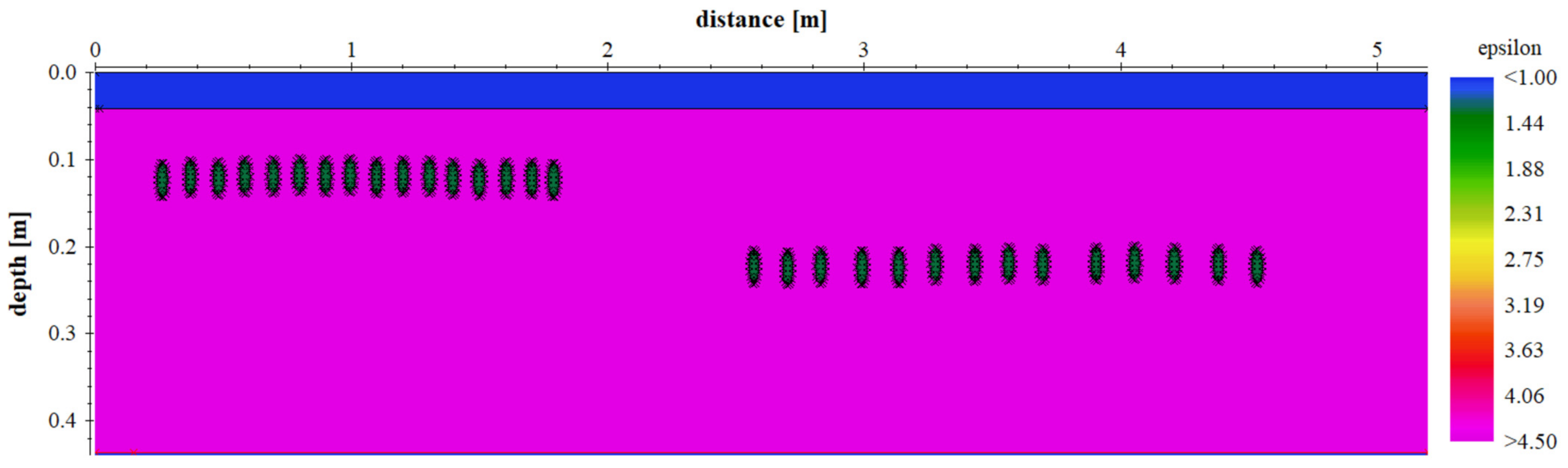
where εr is the relative permittivity, n is the layer, Ao is the amplitude of the air, and Amax is the maximum amplitude of the reflected signal. To use this equation, we needed to assume that the layer is homogeneous; thus, there is no lateral and vertical variation within the same layer, unless there is another feature inside it. The geometry of the tunnel lining and rebars are shown in Figure 7 and Figure 8, respectively. Figure 7 shows four layers, such as the air layer (εr = 1, d = 0.1 m), the second lining (εr = 6, d = 0.5 m), the first lining (εr = 10.5, d = 0.2 m), and the wall rock (εr = 13, d = 0.3 m), these layers are in the box, where the distance of the x direction is 1 m and the depth is 1.1 m based on the prior information in the field data. Figure 8 shows the model for the rebars with x = 5.2 m and depth or y = 0.44 m. It consists of two layers: the air layer, with relative permittivity (εr) = 1, relative magnetic permeability (μr) = 1, and electrical conductivity (σ) = 0 S/m, and the second lining, with εr = 6, μr = 1, and σ = 1 × 10⁻³ S/m. The rebars model are placed inside the second lining, with radius (r) = 0.02 m, εr = 1.45, μr = 1000, and σ = 100 S/m.
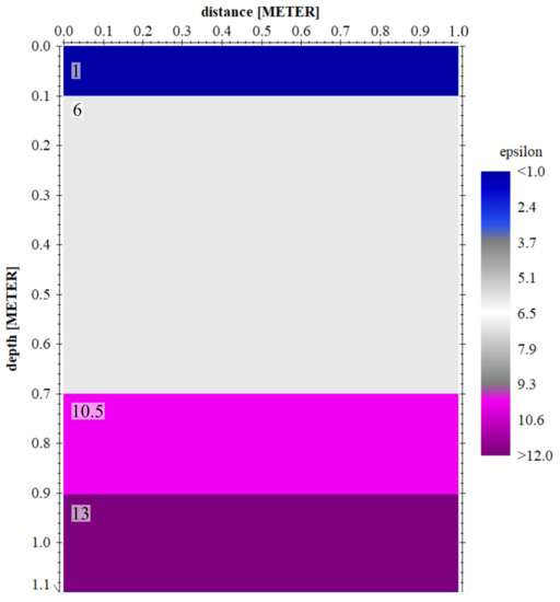
Figure 7.
The geometry of the TDFM for the lining boundary simulation. It consists of four layers with different permittivities (ε).

Figure 8.
The geometry of the TDFM for the rebars simulation. It consists of two layers, where the blue layer is the air and the magenta layer is the second lining. The rebars with the blue circle are placed inside the second layer.
3. Results
3.1. The Lining of The Tunnel
Although we scanned 10 tunnels, we obtained 26 radargrams, due to the tunnel’s condition (Table 1). Sometimes, in the same tunnel, we needed to stop due to the fact that the GPR antennas were too close to the surface of the tunnel, so we adjusted the versatile holder to avoid the antennas bumping into the surface of the tunnel (this is one of the advantages of our VMGPR system) and started over again. The radargram revealed that the lining of the tunnel consists of three layers: the second lining, the first lining, and the wall rock (Figure 4). However, another additional layer was found before the second lining, and we interpreted it as the air layer. It appeared due to the distance of the antennas and the surface of the wall; if the antennas are close to the surface wall, the air layer is thin, and vice versa.

Table 1.
The thickness of the tunnel lining in the SLRT.
3.2. The Rebar Inside the Second Lining
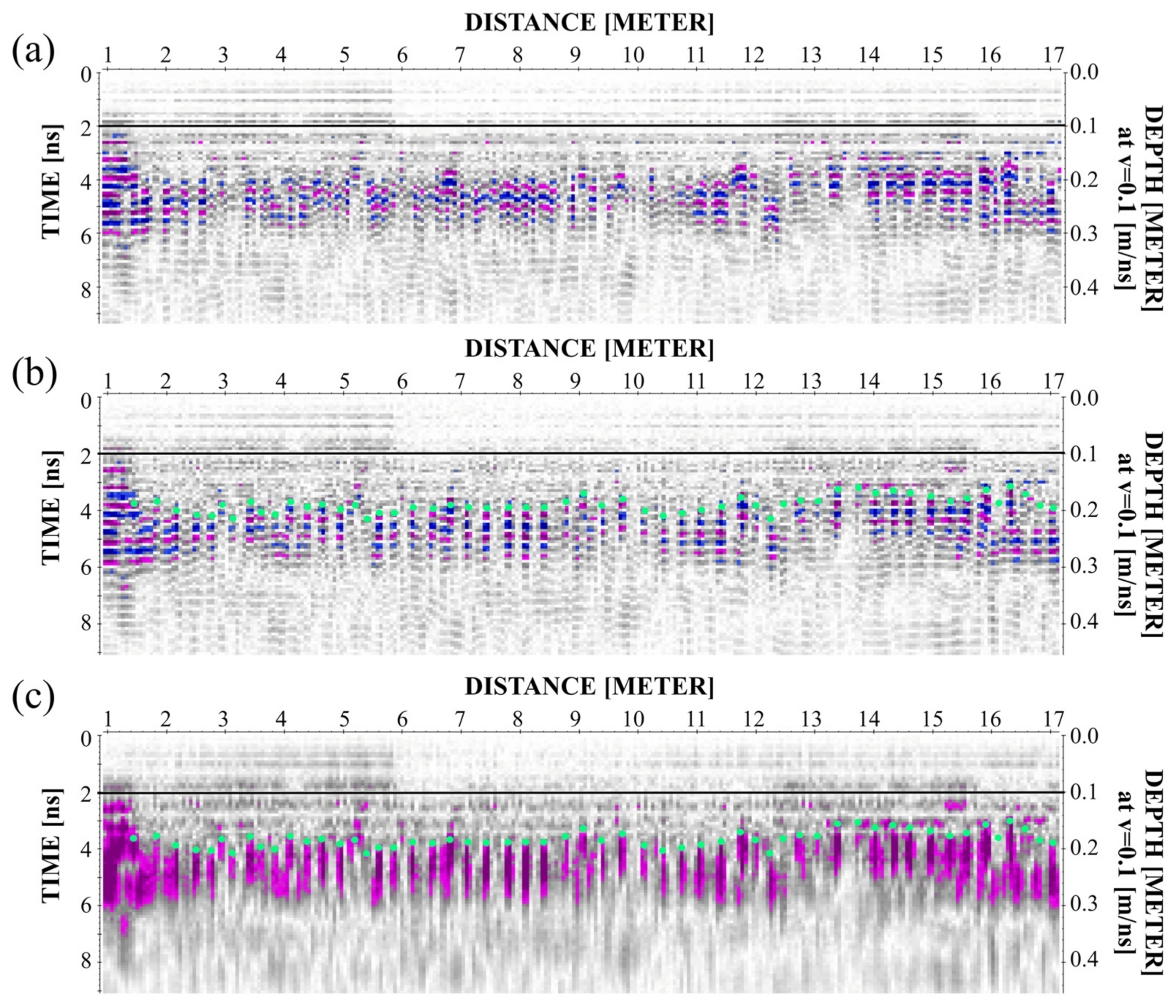
The rebar in the tunnels was mainly found in the second lining, and was approximately 0.1 m below the surface. Figure 9 shows an example from the Fangdian 1 tunnel. Numerous small hyperbolic patterns were visible in the radargram embedded in the concrete screed, identified as the responses of the rebar (Figure 9a). Figure 9b,c shows the post-processing results, where the FK-migration and the HT were applied in order to enhance the results. We used similar steps with the tunnel lining detection in order to find the interface of the second lining and the rebar.
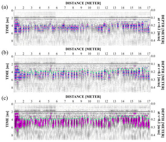
Figure 9.
(a) Radargram in the Fangdian 1 tunnel. Numerous small hyperbolic patterns were visible in the radargram embedded in the concrete screed, identified as rebar responses; (b) radargram with rebar responses after FK migration. The green dots are the interface of the rebar and the second lining; (c) radargram after Hilbert Transform (HT) to calculate the instantaneous amplitude or envelope. Strong amplitude (the magenta color) as a response of the rebar reflection.
3.3. The Result of TDFM
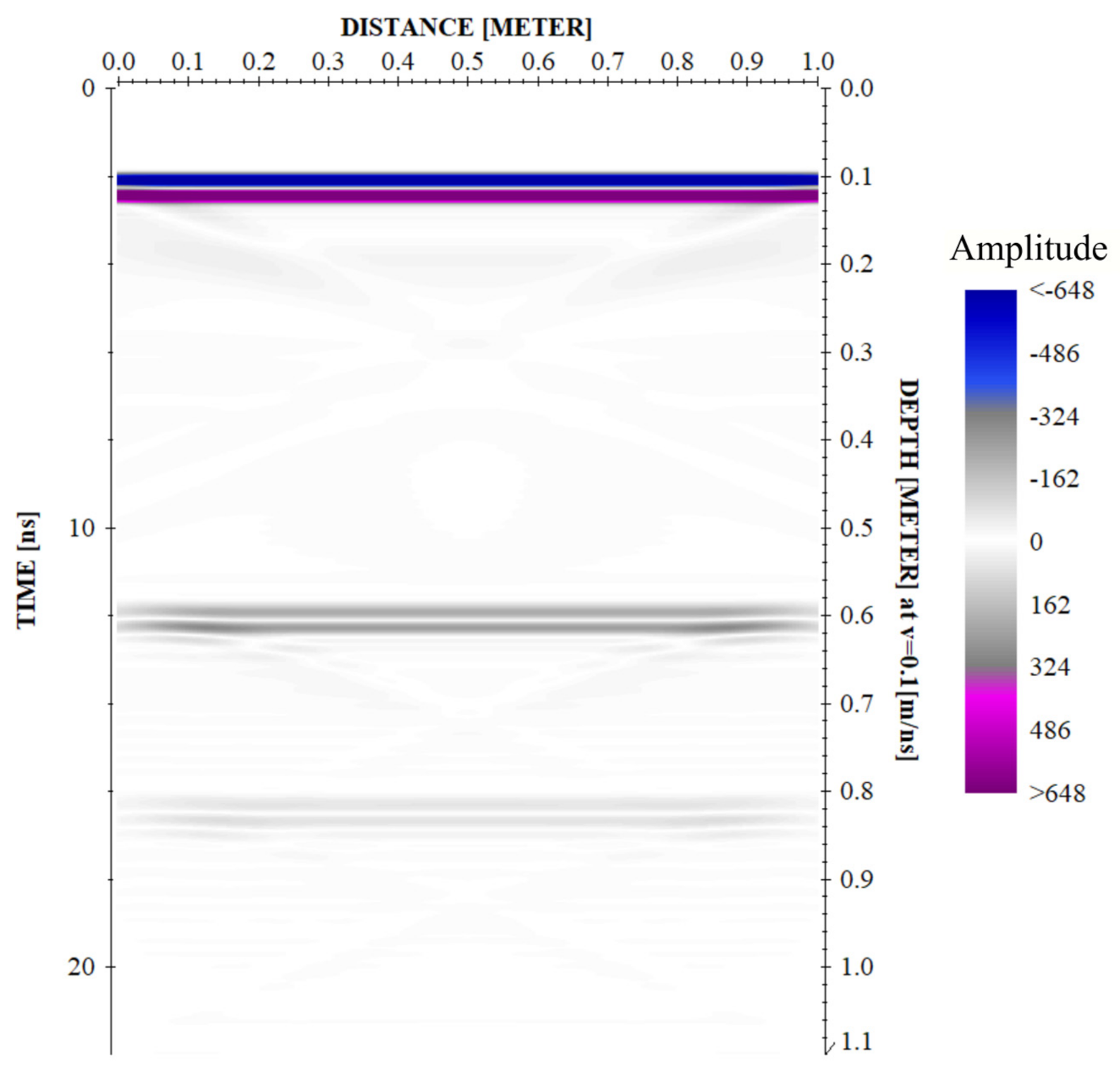
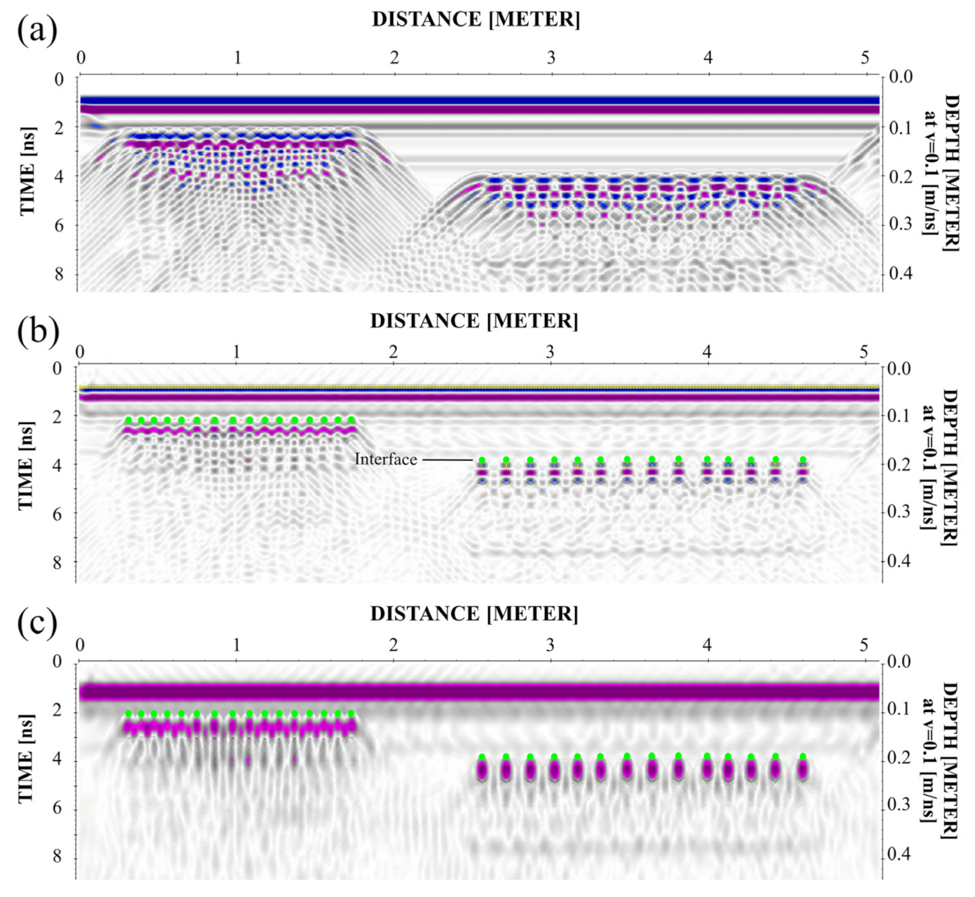
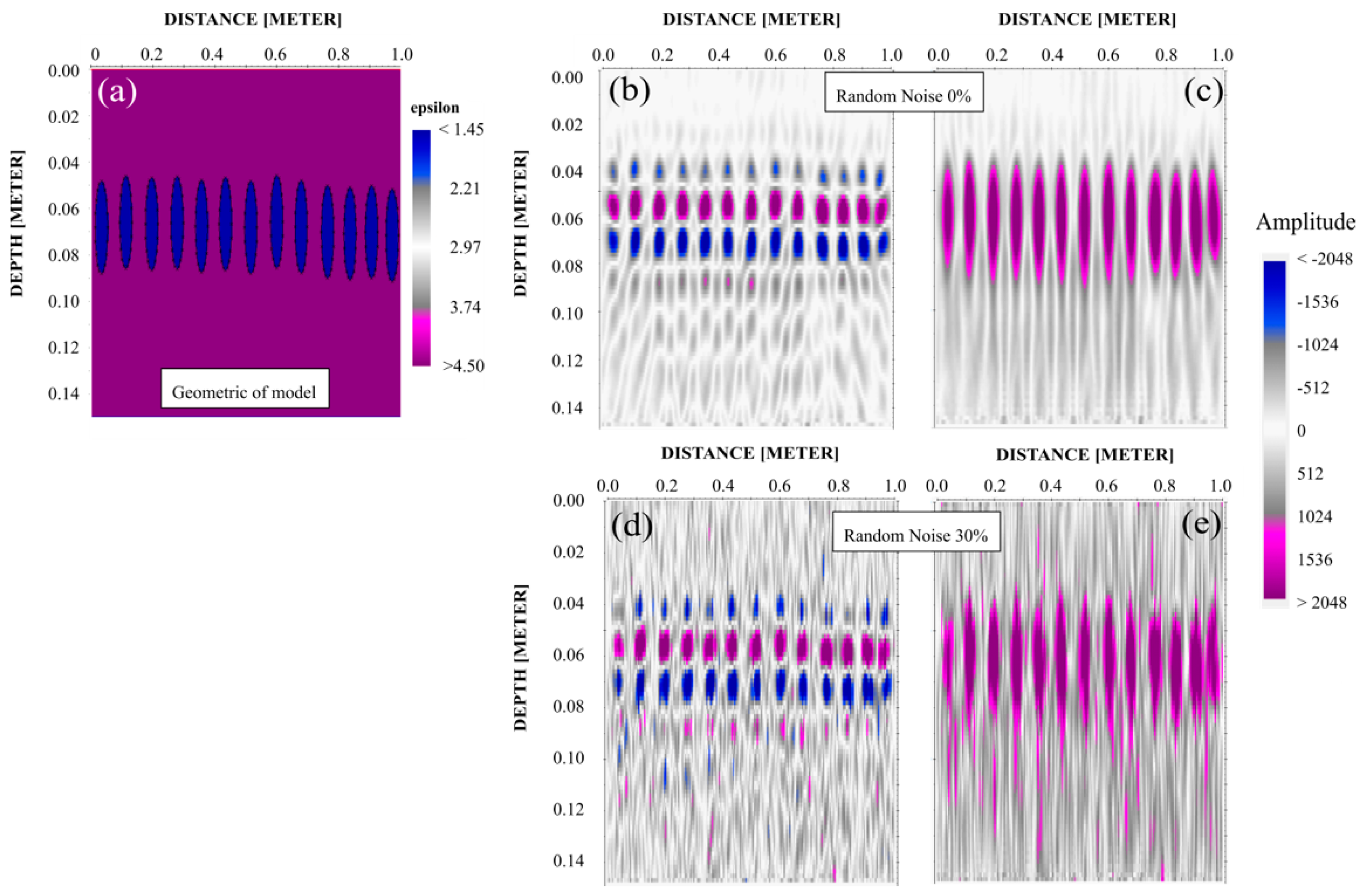
The results of the TDFM for the tunnel lining and the rebar are shown in Figure 10 and Figure 11, respectively. Figure 10 shows the ideal condition model, which means that no noise influences the data, where the blue line is the negative phase and the magenta line is the positive phase. It is intended to determine the actual condition of the phase of a wave when it propagates into layers with different ε, and the result revealed that the phases of all of the interfaces are negative (ε1 < ε2 < ε3 < ε4). Figure 11a shows the result from the rebar model before being processed, where it is shown that the location of the rebar is hard to interpret due to the fact that the multiple and hyperbolic responses are connected to each other. We included FK migration to correct the right position of the reflectors (Figure 11b), so that the responses of the rebar become clear and easy to interpret. Here, we picked the positive phase as the interface between the second lining and the rebar due to the higher relative permittivity of the second lining compare to the rebar (ε1 > ε2). Furthermore, we applied the HT (Figure 11c) to enhance the responses of the signal, where the negative frequency components are shifted by −90 degrees. In addition, we simulated the TDFM with additional random noise from 0%, to 30% to analyze the influence of the noise on the GPR data, as shown in Figure 12. The geometry of the model is shown in Figure 12a, where we adopted the condition of the field data. The blue color is the rebar and the magenta color is the second lining. After all, we processed the model until we obtained the filtered radargram with the HT, while we added the random noise during the processing step. Figure 12b,d show the filtered radargram with random noise, whereas Figure 12c,e show the filtered radargram after the HT with random noise.

Figure 10.
The radargram from the TDFM with three-layer boundaries.
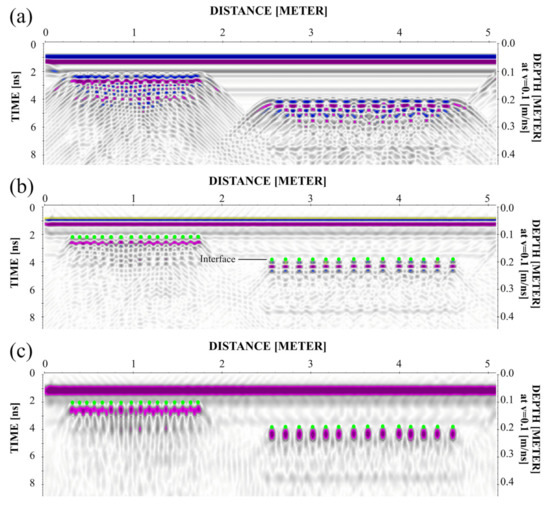
Figure 11.
(a) The radargram (raw data) from the TDFM for the rebar simulation; (b) radargram after FK migration. The green dots are the interface of the rebar and the second lining; (c) radargram after envelope or instantaneous amplitude with Hilbert Transform (HT). Strong amplitude with the magenta circle as a response of the rebar reflection.
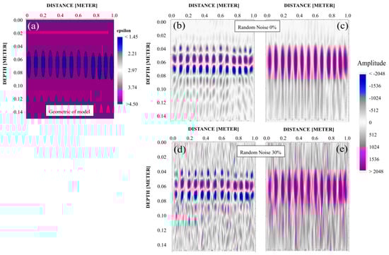
Figure 12.
(a) The geometry model for the rebar simulation in TDFM. It is used for the HAC; (b) filtered radargram with 0% of random noise; (c) radargram b with HT; (d) filtered radargram with 30% of random noise; (e) radargram d with HT.
3.4. The Result of the HAC
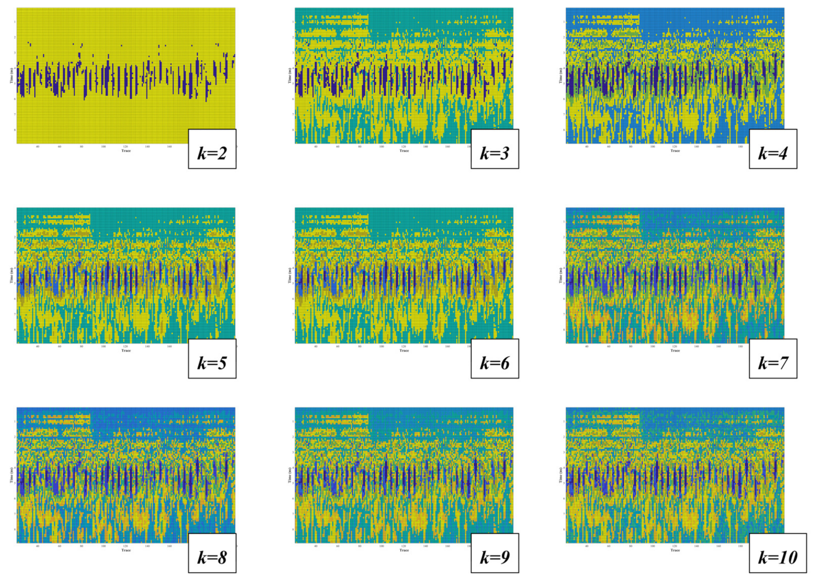
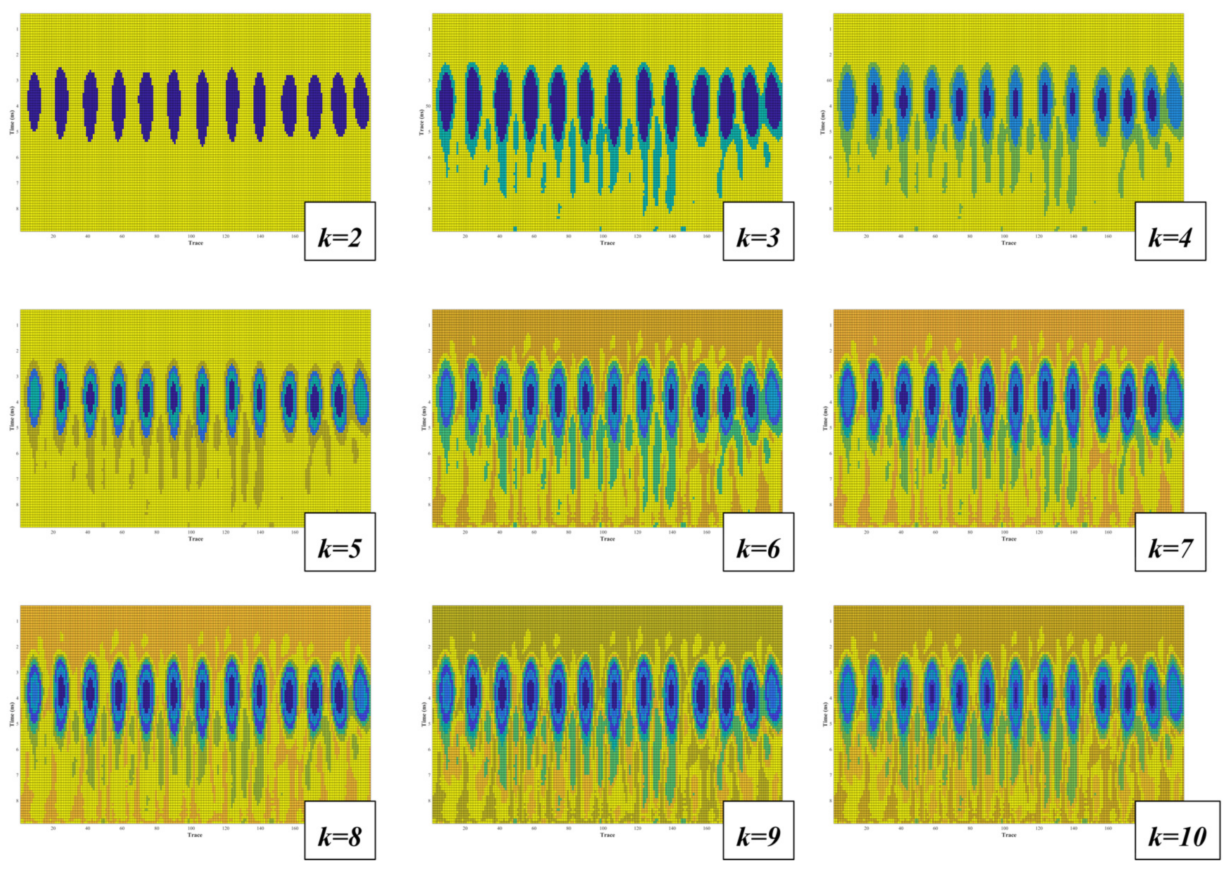
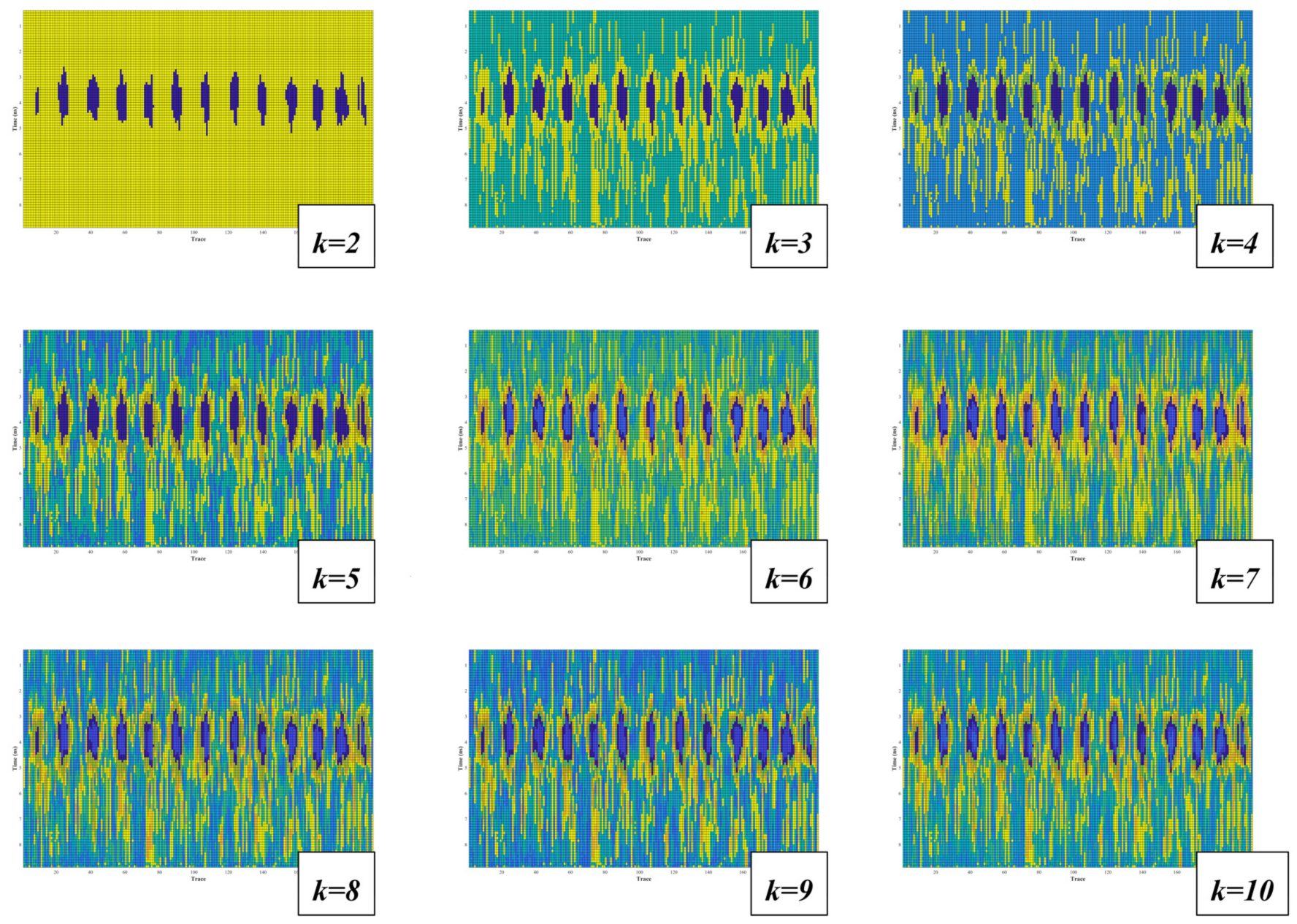
We processed both the field data and the TDFM for the rebar automatic identification. As an example, we used Figure 9c from the Fangdian 1 tunnel. Using Equations (8) and (9), we were able to translate the 2D radargram into a 2D clustered radargram. We produced nine of them with a different number of clusters (k = 2–10). Figure 13 shows the clustered radargram for the field data, where the blue color is the rebar inside the second lining. Furthermore, we processed the TDFM radargram based on the model from Figure 12 to understand the influence of the different random noise, and produced 36 clustered radargrams. Figure 14 and Figure 15 show the clustered radargram for the TDFM data with 0% and 30% random noise, respectively. Similar to the field data, the blue color also represents the rebar inside the second lining.

Figure 13.
The result from the HAC for the field data. There are nine clusters (k) from k = 2 to k = 10.
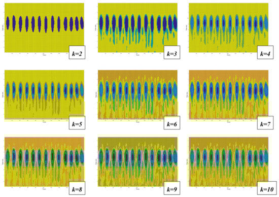
Figure 14.
The result from the HAC for the TDFM data with 0% random noise. There are nine clusters (k) from k = 2 to k = 10.
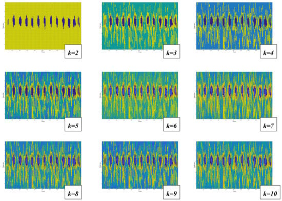
Figure 15.
The result from the HAC for the TDFM data with 30% random noise. There are nine clusters (k) from k = 2 to k = 10.
4. Discussion
Conducting an extensive study of the tunnel lining detection and rebar identification undertaken by the GPR method in the actively operating railway route required a great deal of precise work. Several aspects need to be considered in order to obtain a comprehensive result, such as the system and processing steps. This study found that the VMGPR worked very effectively during the scanning process. Due to its versatility, the occurrence of damage to both the GPR instrument and the surface of the tunnel can be minimized.
The boundary of each lining can be found on the radargram in the form of a series of strong reflection stripes. These distinguishable stripes are caused by multiple individual reflections, which originate in the interface between each layer due to different electromagnetic properties. The more the relative permittivity of two media varies, the bigger the color contrast. For example, the difference in relative permittivity between the air and the second lining is greater than the rest of the interface (Figure 5a). Hence, the color contrast between these two is brighter than the others. A similar conclusion was reached by the TDFM result in Figure 10. Three boundaries can be found, where the first one with the brightest contrast is the boundary between the air (εr = 1) and the second lining (εr = 6), the second one is the boundary between the second lining and the first lining (εr = 10.5), and the third one with the least contrast is the boundary between the first lining and the wall rock (εr = 13.5). Besides, this behavior can occur due to the attenuation of the EM wave. As the wave propagates in the medium, it suffers from attenuation and distortion as a result of spherical spreading, absorption, and dispersion. Daniels [33] provided a list of attenuations of various materials measured by the GPR. The attenuation in the air is 0 dB/m, the attenuation in the concrete dry is in the range of 2–12 dB/m, and the attenuation in the concrete wet is in the range of 10–25 dB/m. Using this information, we concluded that attenuation increases with depth, and thus, the amplitude becomes small and the contrast decreases.
After the boundary is determined, the thickness of each lining (d) is estimated. Table 1 lists our estimation of d for each tunnel. The average thickness of the second lining and the first lining is in the range of 0.41–0.50 m and 0.19–0.26 m, respectively. Overall these findings are in accordance with the findings reported by Lee and Wang [2] and Wang, Chang [1], where the concrete lining in the SLRT tunnels was approximately 0.30–0.55 m thick and had a compressive strength of around 210 MPa. Essentially, the thickness of the second lining should be the same along the tunnel. However, we observed on the radargram that some parts of the lining were thinning. In order to assess this problem, we classified the tunnel according to the total distance of the thinning lining over the total length of the tunnel using Equation (12),
where TL(x) is the percentage of the thinning lining in the tunnel (%), LTL(x) is the total length of the thinning lining ≥ 0.05 m (m), and TLT (x) is the total length of the tunnel (m); the result is listed in Table 2. It is revealed that all of the tunnel is in category A, with the total thinning layer in the range of 0–1.71%, except for the Fangye 1 tunnel with 19.39% (category B). Hence, this tunnel will be further inspected by the engineer.
Table 2.
The classification of the tunnel based on the percentage of the thinning lining.
After the filtered radargram was carried out, we then applied the Hilbert Transform (HT) to enhance our data by extracting the pulse envelope. Figure 9c and Figure 12c are the examples for the HT implementation for the field data and the TDFM data, respectively. The envelope not only gives us an overview of the energy distribution of the traces, but also makes it easier for us to determine the signal’s first arrival, without getting involved with the different phases of the amplitude, since the HT shifts the phase of a signal by 90 degrees. This means that the positive frequency components are shifted by +90 degrees, and vice versa. Besides, this transformation helps us to uniform the data without any phase difference as the data input for the clustering process.
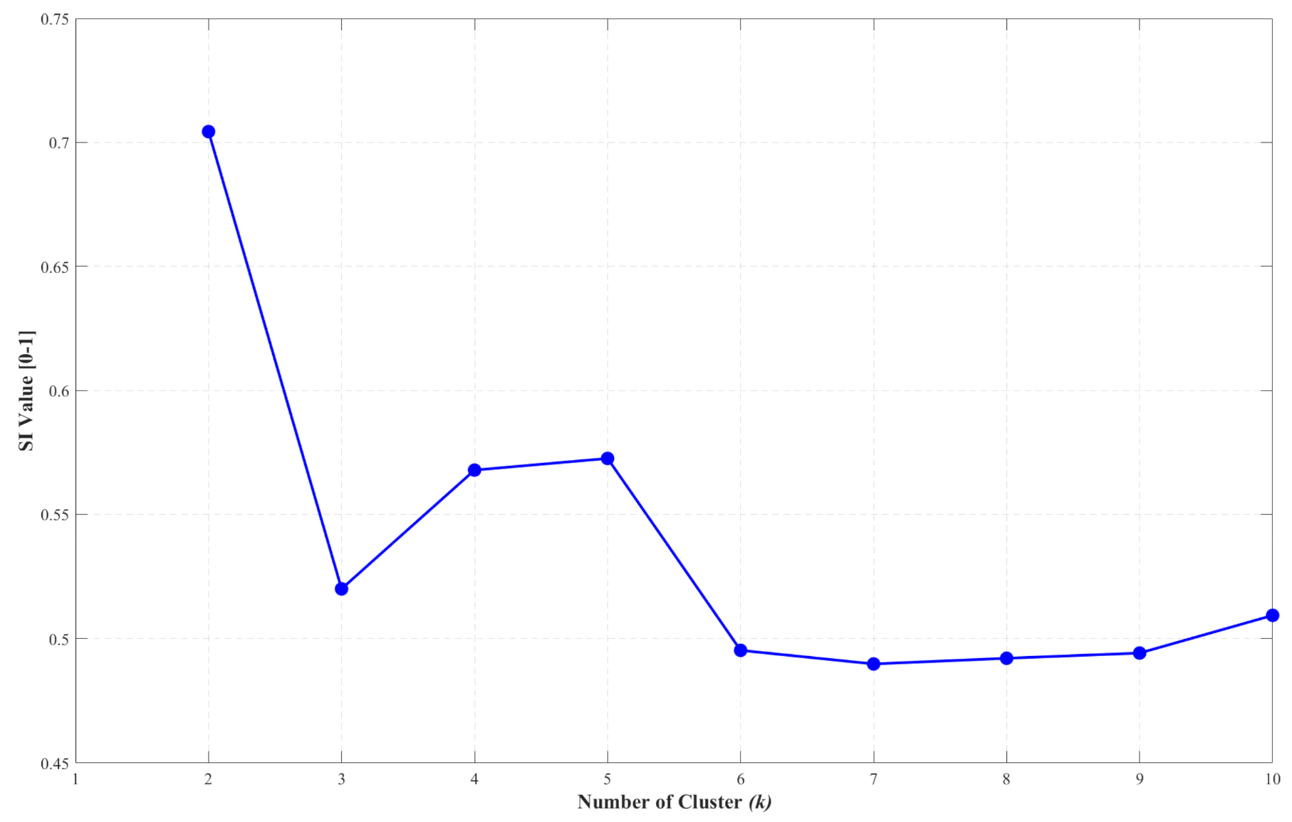
We successfully identified the rebars using Hierarchical Agglomerative Clustering (HAC). Figure 13 shows the field data with nine clusters (k = 2–10), where the rebars are identified as at around 4 ns or at a 0.2 m depth on the clustered radargram, and are marked with a blue color. Even though the number of clusters increases, the rebars are still distinct, on account of the high amplitude compared to the surrounding lining. However, it is interesting to see that the shape of the rebars is irregular in every clustered radargram. In our view, this could have occurred due to the high rate of noise on the data. To assess and confirm this finding, the radargram was simulated. Figure 14 presents a clustered radargram from the TDFM with 0% random noise. We found that this result is in line with the field data, where the rebars can be identified in the middle of the clustered radargram and are marked with a blue color. This test highlighted that the rebars are plainly visible in every number of clusters (k = 2–10) in conformity with the field data (Figure 13), yet the simulation failed to describe the irregular shape of the rebars. In order to see the effect of the noise on the rebars, we gradually added random noise to the model from 0% to 30%. Figure 15 shows a clustered radargram from the TDFM with 30% random noise. Significantly, this result can describe the irregular shape of the rebars in the field data, which means that the noise has affected the shape of the rebars on the radargram; this result concurs with our initial findings. Since clustering algorithms define clusters that are not known a priori information, the final partition of data requires some kind of evaluation method in most applications, including this study. Using Equation (11), we were able to evaluate the results and determine the optimal number of clusters (k) simultaneously, because it can measure the quality of the clustering result (Section 2.4.2). Figure 16 presents the Silhouette Index (SI) curve for the field data, where the highest average SI with 0.704 is k = 2. A similar pattern of results was obtained in TDFM, as shown in Figure 17, where the average SI for each model with various random noise shows that the optimal number of clusters is k = 2, where the dark blue color is the response of the rebar and the rest is the response of the surrounding lining, as shown in Figure 13, Figure 14 and Figure 15.
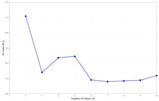
Figure 16.
The average silhouette index (SI) for the field data. k = 2 has the highest average SI, i.e., 0.704.
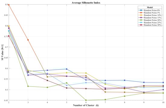
Figure 17.
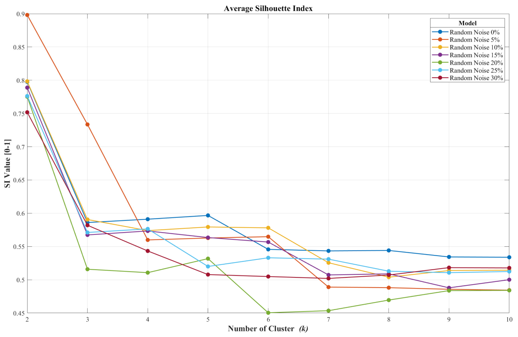
The average silhouette index (SI) for the rebar simulation with random noise (0–30%) in the TDFM. The models with random noise 0%, 5% 10%, 15% 20%, 25%, and 30% have the average SI value for k = 2, i.e., 0. 98, 0.898, 0.798, 0.789, 0.775, 0.776, and 0.752, respectively.
The models with random noise 0%, 5% 10%, 15% 20%, 25%, and 30% have the average SI value for k = 2, i.e., 0. 98, 0.898, 0.798, 0.789, 0.775, 0.776, and 0.752, respectively. Our finding appears to be well substantiated with the TDFM results, which makes sense, since the model is built based on the field data, where the rebar is placed inside the second lining. The most striking result from the TDFM is that the model with noise can mimic our field data. The more noise we added into it, the rougher the shape of the rebar that was obtained. Apart from this slight discordance with other models, the TDFM with 30% random noise seems to describe our field data well, which means that it contained ≥30% noise. We tried several methods to remove it; however, excessive editing may result in a loss of the actual features of the target. Despite this condition, we still can distinguish the rebar and the lining well. There are two limitations in this study that could be addressed in future research. First, several radargrams contain strong multiples in response to the tunnel walls being covered by the waterproof membrane, which make them difficult to analyze. We tried several ways to suppress the multiples, but they could not be completely eliminated. Second, it is difficult to simulate the noise of the field data on the model from TDFM. In this study, we simply added random noise into the model, so conducting further study is needed. Despite the limitations of this study, our findings are capable of detecting the lining of the tunnel and identifying the rebar.
5. Conclusions
We have presented the implementation of the Vehicle-mounted Ground Penetrating Radar (VMGPR) method in the 10 tunnels along the South-link Line Railway of Taiwan (SLRT) in order to both detect the tunnel lining boundary with a comprehensive method and identify the rebar with the Hierarchical Agglomerative Clustering (HAC) in machine learning. The tunnel lining boundary was detected based on the Fresnel Reflection Coefficient (FRC) and was verified with Two-dimensional Forward Modeling (TDFM). Taken together, these results suggest three boundaries of the tunnel lining: the air–second lining boundary, the second–first lining boundary, and the first–wall rock boundary. Then, we determined the lining thickness of each tunnel, where the average thickness for the second lining and the first lining is in the range of 0.41–0.50 m and 0.19–0.26 m, respectively. We then estimated the thickness of the thinning layer in the tunnels, where we found that the Fangye 1 tunnel is the only tunnel in category B, with 19.39% of its second lining being thinned, while the other tunnels are still in category A (0–1.71%). By applying the Hilbert Transform (HT), the interface of each target is easy to detect because it shifted the phase of the signal by 90 degrees, and the overview of the energy distribution of the data is obtained. Moreover, the HT radargram is useful as the input data for the clustering process, where the phase of the amplitude can be neglected.
We have described the procedure for the HAC method to identify the rebar. Both the field data and the TDFM model with different random noise (0–30%) are processed. We evaluated the clustering result and found the optimal number of clusters (k) with the Silhouette Index (SI). The findings suggest that the TDFM model is consistent with the field data, where k = 2 is the best choice to represent our data set. Moreover, according to the HAC result, the TDFM model can mimic the field data. We have found that the TDFM model with 30% random noise seems to describe our data in a good manner, where the rebar response is rough due to the noise.
6. Patents
“Antenna Holder Device for Ground Penetrating Radar”-Taiwan Patent No. M612652–Date of Patent: 1 June 2021.
Author Contributions
Conceptualization, J.M.P. and P.-Y.C.; methodology, J.M.P. and P.-Y.C.; formal analysis, J.M.P.; data curation, J.M.P., P.-Y.C. and D.-J.L.; writing—original draft preparation, J.M.P.; writing—review and editing, J.M.P. and P.-Y.C.; visualization, J.M.P. and H.H.A.; project administration, D.-J.L.; supervision, P.-Y.C. and Y.G.D. provided comments on results discussions with the other authors. All authors have read and agreed to the published version of the manuscript.
Funding
This research was funded by the Minister of Science and Technology (MOST) of Taiwan under the project number of MOST 108-2638-E-008-001-MY2.C and also supported by the industry–academia cooperation between Changsheng Construction Co., Ltd. and Earthquake-Disaster, Risk Evaluation and Management Centre (E-DREaM), under the project number of 10810067.
Data Availability Statement
Data will be available upon request to the authors.
Acknowledgments
We would like to thank Xuan-Chen Zhou from the Changsheng Construction Co., Ltd. for his help during the data acquisition in the tunnel.
Conflicts of Interest
The authors declare no conflict of interest.
References
- Wang, Y.T.; Chang, P.; Lee, Y.; Lee, M. Safety inspection and reinforcement of South-link line railway tunnels. In Proceedings of the 16th Asian Regional Conference on Soil Mechanics and Geotechnical Engineering, Taipei, Taiwan, 14–18 October 2019. [Google Scholar]
- Lee, C.H.; Wang, T.T. Rock tunnel maintenance in Taiwan. In Proceedings of the 6th Asian Young Geotechnical Engineers Conference-2008, Bangalore, India, 20–21 December 2008; pp. 205–217. [Google Scholar]
- Hsu, C.-H.; Tsao, T.-C.; Huang, C.-M.; Lee, C.-F.; Lee, Y.-T. Using Remote Sensing Techniques to Identify the Landslide Hazard Prone Sections along the South Link Railway in Taiwan. Procedia Eng. 2016, 143, 708–716. [Google Scholar] [CrossRef] [Green Version]
- TRA (Taiwan Railways Administration). Available online: https://www.railway.gov.tw/en/ (accessed on 29 June 2021).
- Chen, C.H. Geological Map of Taiwan; Central Geological Survey: Taipei, Taiwan, 2000. [Google Scholar]
- Chandra, S.; Agarwal, M.M. Railway Tunnelling. In Railway Engineering, 2nd ed.; Oxford University Press: Oxford, UK, 2013; pp. 543–561. [Google Scholar]
- Bickel, J.O.; Kuesel, T.R.; King, E.H. Tunnel Engineering Handbook, 2nd ed.; Springer Science & Business Media: Berlin/Heidelberg, Germany, 1996. [Google Scholar] [CrossRef]
- Parkinson, G.; Ékes, C. Ground penetrating radar evaluation of concrete tunnel linings. In Proceedings of the 12th International Conference on Ground Penetrating Radar, Birmingham, UK, 15–19 June 2008. [Google Scholar]
- Li, C.; Li, M.-J.; Zhao, Y.-G.; Liu, H.; Wan, Z.; Xu, J.-C.; Xu, X.-P.; Chen, Y.; Wang, B. Layer recognition and thickness evaluation of tunnel lining based on ground penetrating radar measurements. J. Appl. Geophys. 2011, 73, 45–48. [Google Scholar] [CrossRef]
- Xiang, L.; Zhou, H.-l.; Shu, Z.; Tan, S.-h.; Liang, G.-q.; Zhu, J. GPR evaluation of the Damaoshan highway tunnel: A case study. NDT E Int. 2013, 59, 68–76. [Google Scholar] [CrossRef]
- Zan, Y.; Li, Z.; Su, G.; Zhang, X. An innovative vehicle-mounted GPR technique for fast and efficient monitoring of tunnel lining structural conditions. Case Stud. Nondestruct. Test. Eval. 2016, 6, 63–69. [Google Scholar] [CrossRef] [Green Version]
- Alani, A.M.; Tosti, F. GPR applications in structural detailing of a major tunnel using different frequency antenna systems. Constr. Build. Mater. 2018, 158, 1111–1122. [Google Scholar] [CrossRef]
- Dinh, K.; Zayed, T.; Moufti, S.; Shami, A.; Jabri, A.; Abouhamad, M.; Dawood, T. Clustering-Based Threshold Model for Condition Assessment of Concrete Bridge Decks with Ground-Penetrating Radar. Transp. Res. Rec. J. Transp. Res. Board 2015, 2522, 81–89. [Google Scholar] [CrossRef]
- Dinh, K.; Gucunski, N.; Duong, T.H. An algorithm for automatic localization and detection of rebars from GPR data of concrete bridge decks. Autom. Constr. 2018, 89, 292–298. [Google Scholar] [CrossRef]
- Dou, Q.; Wei, L.; Magee, D.R.; Cohn, A.G. Real-Time Hyperbola Recognition and Fitting in GPR Data. IEEE Trans. Geosci. Remote. Sens. 2017, 55, 51–62. [Google Scholar] [CrossRef] [Green Version]
- Liang, H.; Xing, L.; Lin, J. Application and Algorithm of Ground-Penetrating Radar for Plant Root Detection: A Review. Sensors 2020, 20, 2836. [Google Scholar] [CrossRef]
- Kilic, G.; Eren, L. Neural network based inspection of voids and karst conduits in hydro–electric power station tunnels using GPR. J. Appl. Geophys. 2018, 151, 194–204. [Google Scholar] [CrossRef]
- Ozkaya, U.; Melgani, F.; Belete Bejiga, M.; Seyfi, L.; Donelli, M. GPR B scan image analysis with deep learning methods. Measurement 2020, 165, 107770. [Google Scholar] [CrossRef]
- Jin, Y.; Duan, Y. Wavelet Scattering Network-Based Machine Learning for Ground Penetrating Radar Imaging: Application in Pipeline Identification. Remote Sens. 2020, 12, 3655. [Google Scholar] [CrossRef]
- Cui, X.; Quan, Z.; Chen, X.; Zhang, Z.; Zhou, J.; Liu, X.; Chen, J.; Cao, X.; Guo, L. GPR-Based Automatic Identification of Root Zones of Influence Using HDBSCAN. Remote Sens. 2021, 13, 1227. [Google Scholar] [CrossRef]
- Chang, P.Y.; Lin, D.J.; Puntu, J.M. Antenna Holder Device for Ground Penetrating Radar. In H01Q-001/00(2006.01); Intellectual Property Office MOEA R.O.C: Taipei, Taiwan, 2021. [Google Scholar]
- Nielsen, F. Introduction to HPC with MPI for Data Science; Springer: Berlin/Heidelberg, Germany, 2016. [Google Scholar] [CrossRef]
- Shyu, J.B.H. Neotectonic architecture of Taiwan and its implications for future large earthquakes. J. Geophys. Res. 2005, 110. [Google Scholar] [CrossRef] [Green Version]
- Ho, C.S. An Introduction to the Geology of Taiwan, Explanatory Text of the Geologic Map of Taiwan, 2nd ed.; Central Geological Survey Taiwan, Ministry of Economy Affairs: Taipei, Taiwan, 1988; p. 192.
- Sandmeier, K.J. Reflexw Version 9.0: Windows XP/7/8/10-Program for the Processing of Seismic, Acoustic or Electromagnetic, Reflection, Refraction and Transmission Data; Sandmeier Geophysical Research: Karlsruhe, Germany, 2019. [Google Scholar]
- Jol, H.M. Ground Penetrating Radar Theory and Applications; Elsevier: Oxford, UK, 2009. [Google Scholar] [CrossRef]
- Benedetto, A.; Tosti, F.; Ciampoli, L.B.; D’amico, F. An overview of ground-penetrating radar signal processing techniques for road inspections. Signal Process. 2017, 132, 201–209. [Google Scholar] [CrossRef]
- Nobes, D.C. Geophysical surveys of burial sites: A case study of the Oaro urupa. Geophysics 1999, 64, 357–367. [Google Scholar] [CrossRef]
- Olhoeft, G.R. Maximizing the information return from ground penetrating radar. J. Appl. Geophys. 2000, 43, 175–187. [Google Scholar] [CrossRef]
- Kim, J.-H.; Cho, S.-J.; Yi, M.-J. Removal of ringing noise in GPR data by signal processing. Geosci. J. 2007, 11, 75–81. [Google Scholar] [CrossRef]
- Maruddani, B.; Sandi, E. The Development of Ground Penetrating Radar (GPR) Data Processing. Int. J. Mach. Learn. Comput. 2019, 9, 768–773. [Google Scholar] [CrossRef]
- Utsi, E.C. Ground Penetrating Radar: Theory and Practice; Butterworth-Heinemann: Oxford, UK, 2017. [Google Scholar] [CrossRef]
- Daniels, D.J. Ground Penetrating Radar, 2nd ed.; The Institution of Electrical Engineer: London, UK, 2004. [Google Scholar] [CrossRef] [Green Version]
- Ismail, M.; Abas, A.; Arifin, M.; Ismail, M.; Othman, N.; Setu, A.; Ahmad, M.; Shah, M.; Amin, S.; Sarah, T. Integrity inspection of main access tunnel using ground penetrating radar. IOP Conf. Ser. Mater. Sci. Eng. 2017, 271, 012088. [Google Scholar] [CrossRef] [Green Version]
- Neal, A. Ground-penetrating radar and its use in sedimentology: Principles, problems and progress. Earth-Sci. Rev. 2004, 66, 261–330. [Google Scholar] [CrossRef]
- Tong, L.-T. Application of Ground Penetrating Radar to Locate Underground Pipes. Terr. Atmos. Ocean. Sci. 1993, 4, 171–178. [Google Scholar] [CrossRef]
- De Souza, T. Concrete Scanning with GPR Guidebook; Sensors & Software Inc.: Mississauga, ON, Canada, 2013. [Google Scholar]
- Vasudeo, A.; Katpatal, Y.; Ingle, R. Uses of dielectric constant reflection coefficients for determination of groundwater using ground-penetrating radar. World Appl. Sci. J. 2009, 6, 1321–1325. [Google Scholar]
- Zhou, F.; Chen, Z.; Liu, H.; Cui, J.; Spencer, B.F.; Fang, G. Simultaneous Estimation of Rebar Diameter and Cover Thickness by a GPR-EMI Dual Sensor. Sensors 2018, 18, 2969. [Google Scholar] [CrossRef] [PubMed] [Green Version]
- Everitt, B.S.; Landau, S.; Leese, M.; Stahl, D. Cluster Analysis, 5th ed.; John Wiley & Sons, Inc.: London, UK, 2011. [Google Scholar] [CrossRef]
- Ah-Pine, J. An Efficient and Effective Generic Agglomerative Hierarchical Clustering Approach. J. Mach. Learn. Res. 2018, 19, 1615–1658. [Google Scholar]
- Batrakov, D.; Golovin, D.; Simachev, A.; Batrakova, A. Hilbert transform application to the impulse signal processing. In Proceedings of the 2010 5th International Confernce on Ultrawideband and Ultrashort Impulse Signals, Sevastopol, Ukraine, 6–10 September 2010; pp. 113–115. [Google Scholar]
- Zhang, Y.; Venkatachalam, A.S.; Xia, T.; Xie, Y.; Wang, G. Data analysis technique to leverage ground penetrating radar ballast inspection performance. IEEE Radar Conf. 2014. [Google Scholar] [CrossRef]
- Delforge, D.; Watlet, A.; Kaufmann, O.; Van Camp, M.; Vanclooster, M. Time-series clustering approaches for subsurface zonation and hydrofacies detection using a real time-lapse electrical resistivity dataset. J. Appl. Geophys. 2020, 184, 104203. [Google Scholar] [CrossRef]
- Dumont, M.; Reninger, P.A.; Pryet, A.; Martelet, G.; Aunay, B.; Join, J.L. Agglomerative hierarchical clustering of airborne electromagnetic data for multi-scale geological studies. J. Appl. Geophys. 2018, 157, 1–9. [Google Scholar] [CrossRef]
- Xu, S.; Sirieix, C.; Riss, J.; Malaurent, P. A clustering approach applied to time-lapse ERT interpretation—Case study of Lascaux cave. J. Appl. Geophys. 2017, 144, 115–124. [Google Scholar] [CrossRef]
- Genelle, F.; Sirieix, C.; Riss, J.; Naudet, V. Monitoring landfill cover by electrical resistivity tomography on an experimental site. Eng. Geol. 2012, 145–146, 18–29. [Google Scholar] [CrossRef] [Green Version]
- Demsa, J.; Curk, T.; Erjavec, A.; Gorup, C.; Hocevar, T.; Milutinovic, M.; Mozina, M.; Polajnar, M.; Toplak, M.; Staric, A.; et al. Orange: Data Mining Toolbox in Python. J. Mach. Learn. Res. 2013, 14, 2349–2353. [Google Scholar]
- Meng, X.; Xu, Y.; Xiao, L.; Dang, Y.; Zhu, P.; Tang, C.P.; Zhang, X.; Liu, B.; Gou, S.; Yue, Z. Ground-penetrating radar measurements of subsurface structures of lacustrine sediments in the Qaidam Basin (NW China): Possible implications for future in-situ radar experiments on Mars. Icarus 2019, 338, 113576. [Google Scholar] [CrossRef]
- Akinsunmade, A.; Karczewski, J.; Mazurkiewicz, E.; Tomecka-Suchoń, S. Finite-difference time domain (FDTD) modeling of ground penetrating radar pulse energy for locating burial sites. Acta Geophys. 2019, 67, 1945–1953. [Google Scholar] [CrossRef] [Green Version]
- Liu, S.; Zeng, Z.; Deng, L. FDTD simulations for ground penetrating radar in urban applications. J. Geophys. Eng. 2007, 4, 262–267. [Google Scholar] [CrossRef]


Publisher’s Note: MDPI stays neutral with regard to jurisdictional claims in published maps and institutional affiliations. |
© 2021 by the authors. Licensee MDPI, Basel, Switzerland. This article is an open access article distributed under the terms and conditions of the Creative Commons Attribution (CC BY) license (https://creativecommons.org/licenses/by/4.0/).