Subsoil Recognition for Road Investment Supported by the Integration of Geodetic and GPR Data in the Form of a Point Cloud

Abstract

During road construction investments, the key issue affecting the structure’s safety is accurate subsoil recognition. Identifying subsoil variability zones or natural voids can be performed using geophysical methods, and ground-penetrating radar (GPR) is recommended for this task as it identifies the location and spatial range karst formations. This paper describes the methodology of acquisition and processing of GPR data for ground recognition for road investment. Additional subsoil research was performed after karst phenomena were identified in the investment area, formations not revealed by geological recognition from earlier studies during the pre-design stage. Mala Ramac CU II radar with a 250 MHz antenna and a Leica DS2000 with 250 and 700 MHz antennas with real-time geopositioning were used to obtain the data. Regarding GPR data postprocessing, we present a method of converting spatial visualization into a point cloud that allows for GPR and geodetic data integration and confrontation. This approach enabled us to determine the locations of control trenches, the results of which were used for material validation, which is necessary to improve the reliability of subsoil recognition. The results showed a high correlation between the recorded GPR signals and the subsoil structure. Additionally, differences in the quality of results for measurements conducted before laying supporting layers with slag and on the completed road structure surface are illustrated.

1. Introduction

The proper recognition of foundation soil is essential for designing construction investments, both cubature and infrastructure. It increases safety and reduces additional costs at the realization stage and during the exploitation of engineering structures. One of the tools supporting ground recognition is a geophysical survey, which, among other things, recognizes the tectonic structure of the layers during sulfur extraction [1], landslide monitoring in the infrastructure areas [2] and tectonic movements [3]. Several research projects have been conducted on the geometrization of changes to the ground-based on 2D geophysical profiles [4,5,6,7]. The possibility of contouring the boundaries of soil layers allows for a 3D analysis (i.e., determining the range and volume of the identified structures. This is particularly important for ground reinforcement design, stability assessment and soil replacement.

In the field of construction investment, however, the principles of subsoil recognition using geophysical methods are not standardized. In 2015, the Polish General Directorate for National Roads and Motorways (GDDKiA), together with the National Center for Research and Development (NCBiR), under the joint undertaking “Development of Road Innovation”, undertook the task of structuring and adapting the regulations to the current technological state. The outcome of the grant completed in 2018 is a project of “Guidelines for the performance of subsoil research for road construction” [8,9]. The scope of the geophysical methods was included very broadly, from the issues, through the selection of research methods and parameters, to their development and documentation. The recommended research methods included ground-penetrating radar (GPR), although priority was given to electrical resistivity tomography (ERT) due to the possible penetration range.

Geophysical surveys are a form of remote sensing, the accuracy and resolution of which are determined by the influence of the propagation environment on the electromagnetic signal. In the case of GPR, dependence on the value of the recorded signal amplitude on the wave propagation medium is simplified to the electromagnetic wave reflection coefficient Γ, according to the equation [10]:

$$\mathsf{\Gamma }=\frac{\sqrt{{\epsilon }_{r1}}-\sqrt{{\epsilon }_{r2}}}{\sqrt{{\epsilon }_{r1}}+\sqrt{{\epsilon }_{r2}}}$$

(1)

where ε_r1, ε_r2 are the relative electric permeability of the adjacent media.

Distinguishing the boundaries of the medium in GPR is possible when the power of the reflected signal P_Γ is described by the relation (Annan, 2000, 2001):

$$P_{\mathsf{\Gamma }}={\left(\frac{\sqrt{{\epsilon }_{r1}}-\sqrt{{\epsilon }_{r2}}}{\sqrt{{\epsilon }_{r1}}+\sqrt{{\epsilon }_{r2}}}\right)}^2\ge 0.01$$

(2)

As Formula (2) shows, the greater the differentiation of the relative dielectric permeabilities of the adjacent layers, the greater the chance of unambiguously mapping the boundary between them. The relative dielectric permeability of air equals 1, and values for other media are at least three times higher. Such a parameter ratio provides good visualization of voids in natural or anthropogenic forms on radargrams, especially for media with low electrical conductivity (i.e., with a low electromagnetic wave propagation attenuation coefficient).

Due to clutter [11], which interferes with the useful signal [12], or wave attenuation, it is difficult to develop interpretation keys for GPR data even if based on calibration measurements.

Many research examples confirm the relatively high effectiveness of the GPR method in the detection of underground utility networks [13,14] and the localization and diagnosis of shallow crypts and tunnels [15,16,17]. However, some differences between anthropogenic and natural forms should be noted. The examples reported in the mentioned publications presented results obtained on anthropogenic objects with regular shapes. Moreover, the calibration of the results of geophysical surveys carried out on anthropogenic objects can be performed based on information such as the typical geometry of the structure, maps and projects (underground utility networks, road layers, stratified walls, reinforcement elements, flood embankments). The deposition depth of these objects is not large, varying between 2 and 4 m. Similar values were found for typical crypts, cellars and tunnels in both modern and historical buildings.

Among the studies of GPR application to the recognition of natural phenomena, many have referred to the detection of karst formations [18,19,20]. These occur in carbonate rocks for which the relative electrical permeability is in the range of 6–11 [21], which affects the reflection coefficient at a level of 0.42–0.54, and the power of the reflected signal in the range of 0.18–0.29. Therefore, there are favorable conditions for applying GPR at a media boundary like air–rock (especially of high compactness), mainly to detect shallow natural and anthropogenic voids [22,23]. However, for anthropogenic objects such as irregular or unidentified excavations and post-mining voids [24,25], and natural objects, like lithological layers [26] or karst phenomena in the subsoil [26,27], the necessary calibration material is usually information from boreholes. Occasionally, calibration was performed on exposed geological structures in the study area, but this approach also had significant limitations because of edge effects [21].

In areas with varied geological structures, the confrontation of GPR and ERT results is also a subject of research. As in the aforementioned “Guidelines”, some authors underlined the significance and superiority of ERT in the hierarchy of geophysical methods for ground recognition [26,28]. However, the advantage of GPR is that it gives a result with better resolution and efficiently determines the boundaries of materials having large variations in the relative dielectric permittivity of low conductivity, which was emphasized in the publication [29]. 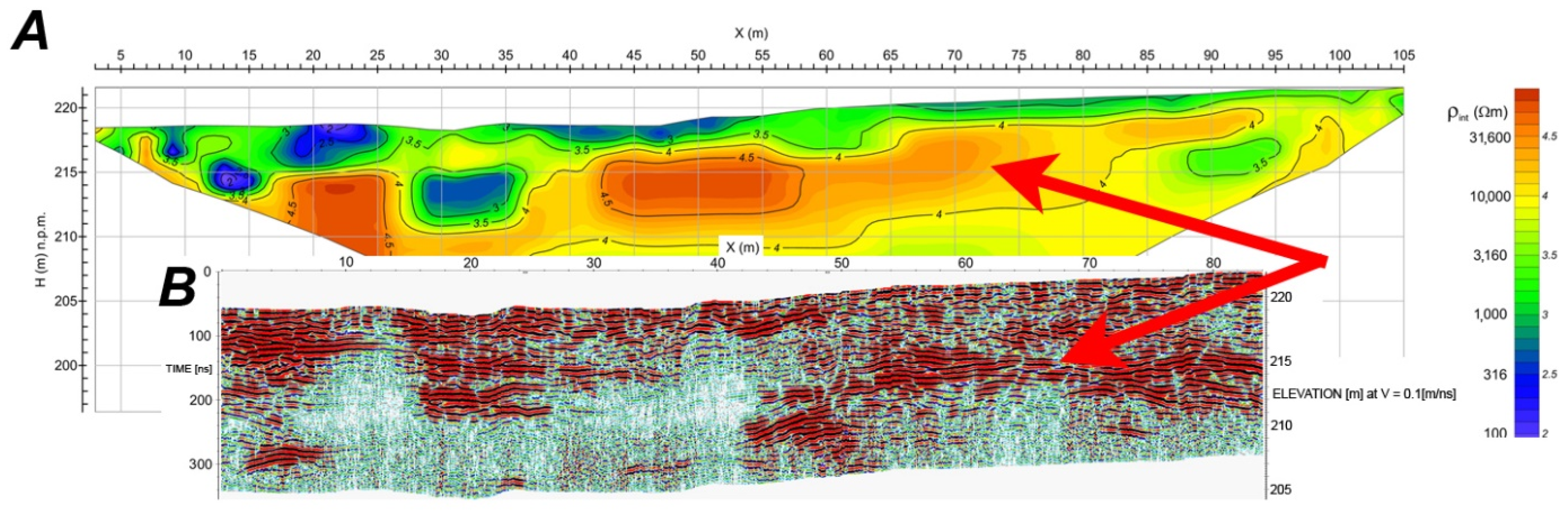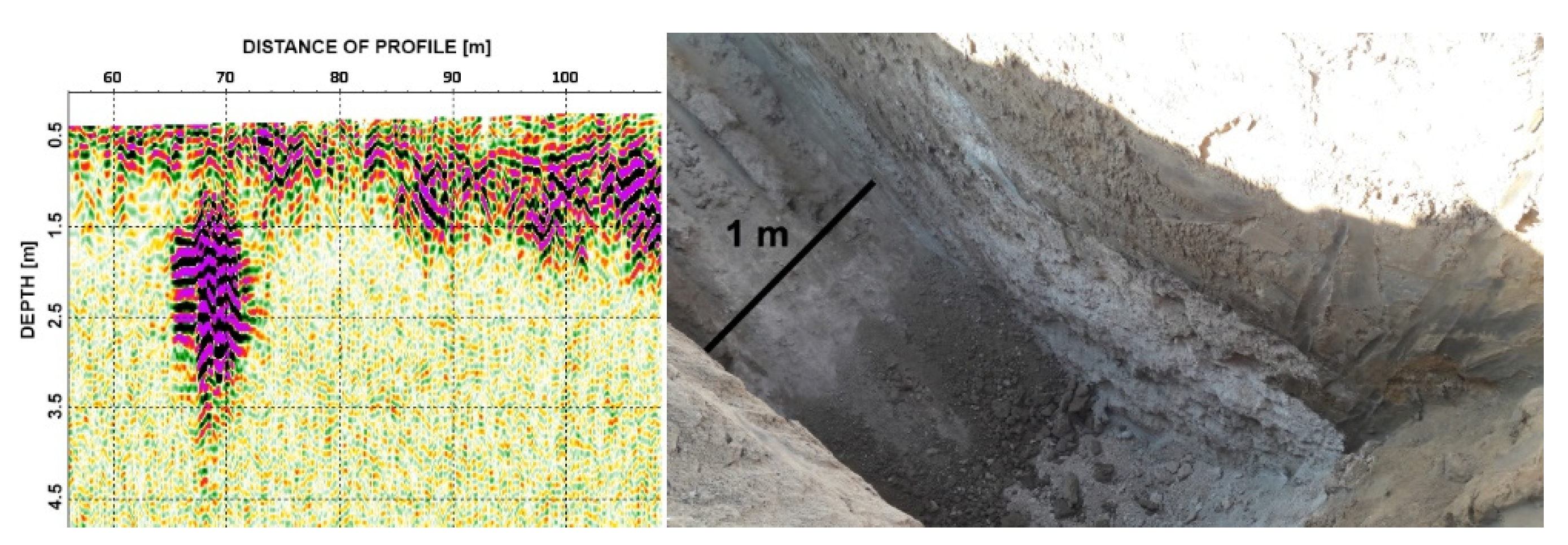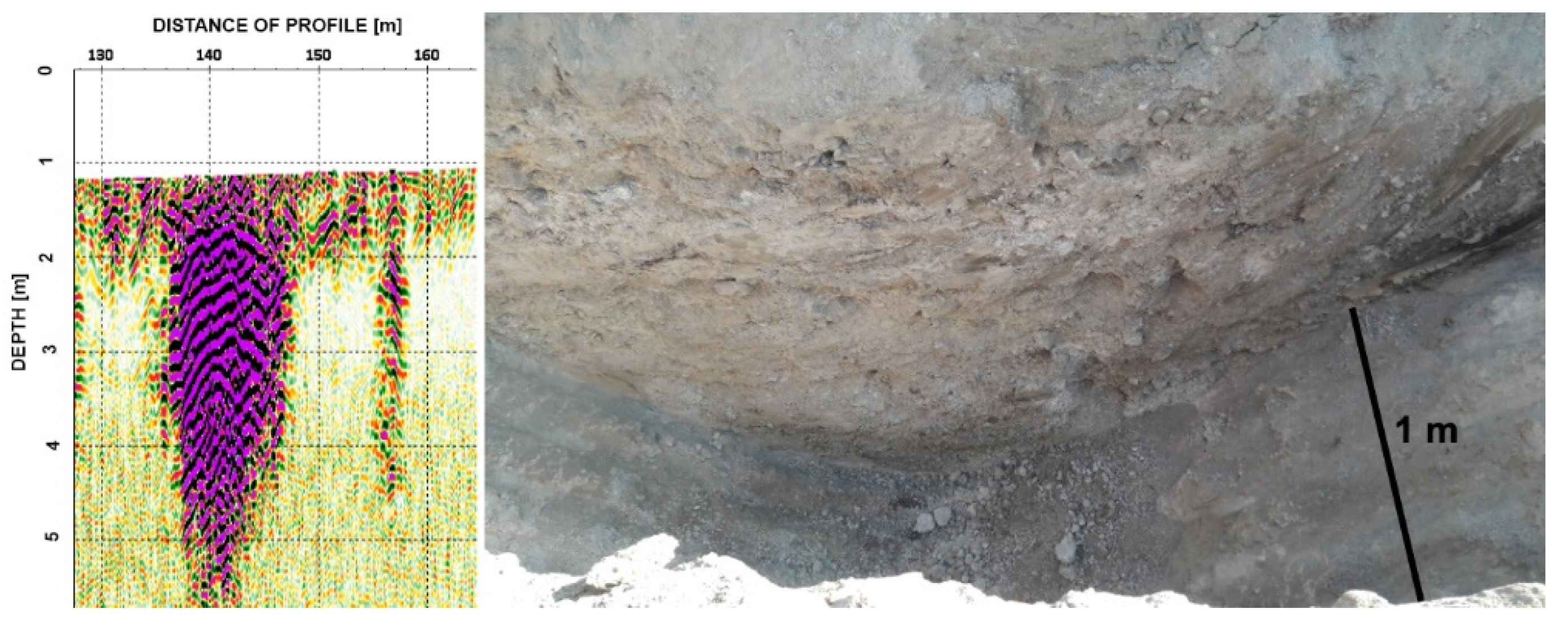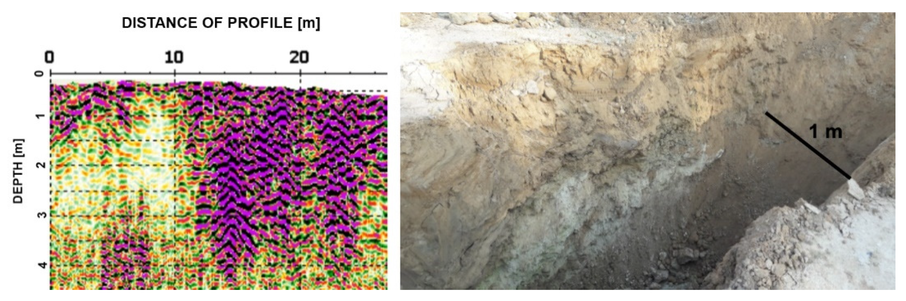In addition, research [30] has noted that GPR was more successful in identifying previously recognized karst phenomena (Figure 1).

According to Ortyl [30], a wide discussion on the application and effectiveness of geophysical methods was carried out. In particular, he investigated the GPR method for recognizing and mapping changes in the structure of the subsoil. Furthermore, an algorithm for converting GPR data into a point cloud file based on geopositioned radargrams was presented. This concept is described as underground radar scanning (UgRS) (Figure 2). Such an approach to GPR data processing eliminates the need for direct access to voids or caves to measure their geometrization and quantification by laser scanning [26,28]. The paper also offered an extensive evaluation of the effectiveness of selected filtering procedures and wave speed calibrations based on terrestrial laser scanning (TLS). Analyses were performed based on synthetic data generated by the Finite Differential Time Domain (FDTD) method and real data.

The following paper is the result of a practical implementation of GPR measurements and data processing to recognize karst formations. During the construction of a national road investment with highway parameters, karst phenomena were identified that had not been indicated in the geological documentation. GPR surveys were carried out on a 7 km section of the newly built road, giving separated areas with different geological structures. Section 2 presents the methodology of data acquisition and postprocessing, in particular the filtering algorithm and the integration of GPR with geodetic data. As a representation of the digital terrain model, the point cloud was acquired using low-range photogrammetry and an unmanned aerial vehicle (UAV). The strong GPR signal responses may have indicated an anomaly caused by a void, rock outcrops, or variations in soil moisture; therefore, post-processing with calibration was required to interpret the GPR data correctly. This paper will then analyze and validate the GPR results based on control trenches with very wide cross-sections. This method allows the exact calibration of the GPR signal response visualization with the actual layout of the ground layers.

2. Materials and Methods

2.1. Description of Research Area

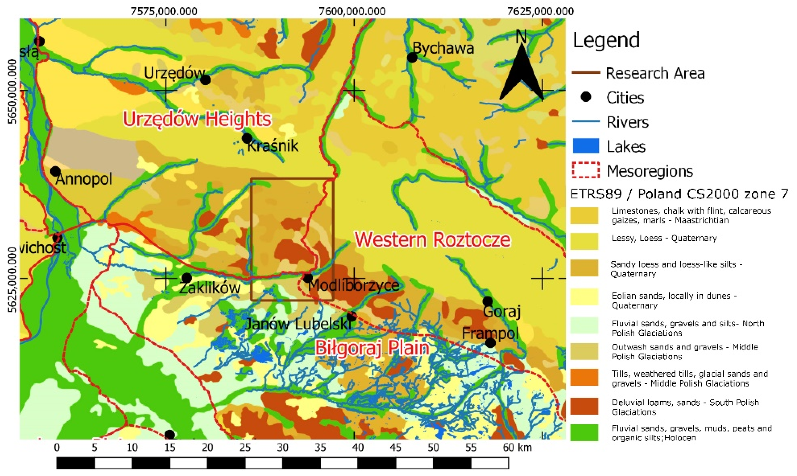
The entire research area was located in the southwestern part of the Lublin Upland, within the mesoregion of Urzędów Heights, close to the border with Western Roztocze and the Biłgoraj Plain. It is a plateau with levelled hilltops cut by river valleys and gullies with steep slopes, which are characteristic of loess areas [31]. The only exposure of Cretaceous and Upper Jurassic formations is located within the Rachowska and Gościeradowa anticlines on a relatively small area. Upper Cretaceous rock predominates, favoring the maintenance of the Tertiary surface plan. The presence of tertiary rocks determines the landscape of the southern part of the region. Especially in the southwestern zone, it is revealed by the stepwise arrangement of monadnock morphological elements [32] (Figure 3).

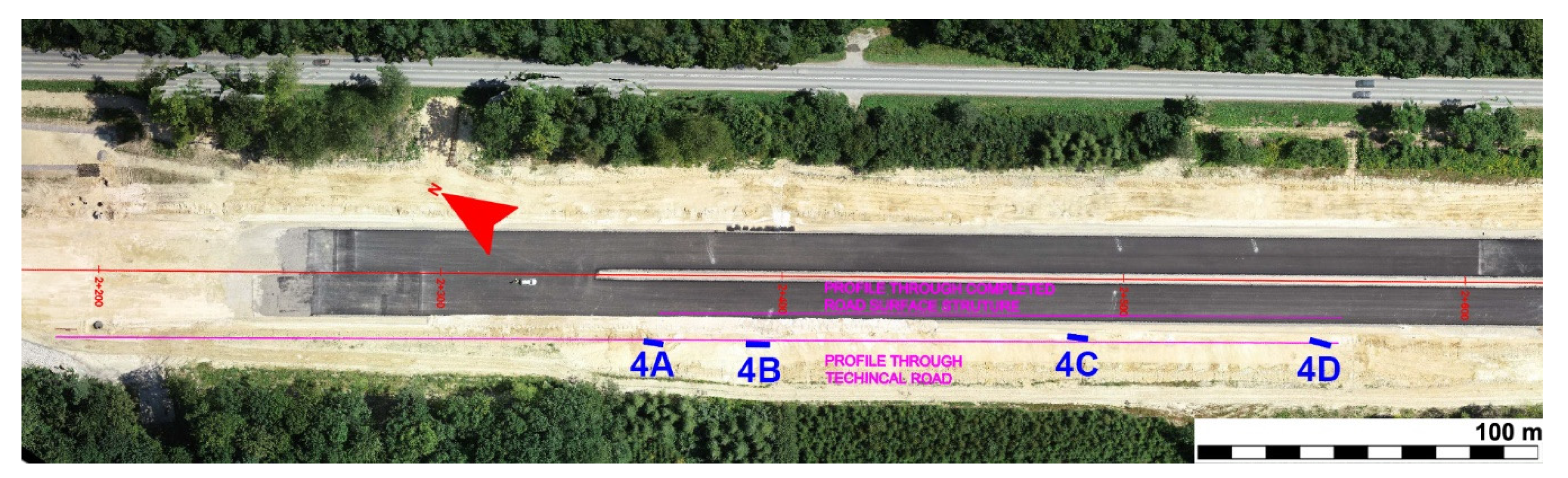
The research area covered the national expressway using the construction parameters of the motorway, which was under construction. GPR and geodetic surveys were carried out on five separate polygons, having a total length of the study route axis of about 2 km distributed over a 7 km length (Figure 4).

2.2. Methodology of Data Acquisition

Field surveys for polygons 1–2 and 4–5 were conducted using Mala RAMAC CU II GPR with a shielded antenna of 250 MHz, which provided an assumed depth of effective penetration up to 5 m. The choice of the antenna frequency was a compromise between the range and resolution of measurements. It enabled ground penetration to capture possible boundaries of native rock, changes in the type of substrate and the presence of karst phenomena. The time window was assumed to be 200 ns, the lowest theoretical speed of electromagnetic wave propagation in limestone equal to 0.09 m/ns, and reached the potential range of penetration up to 8 m. For the highest theoretical speed in limestone (0.12 m/ns), the range increased to 12 m, and echogram traces were recorded at 0.1 m intervals. The signal sampling frequency was 2526 MHz, and the number of signal stacks was assumed to be 32. The Leica TCRA 1002plus robotic tachymeter was used for real-time geopositioning. Measurements were carried out with reference to Poland’s national coordinate system 2000 (CS2000) zone 7, and the Kronstadt’86 height reference frame.

Preliminary analysis of the results from Mala GPR confirmed suitable conditions for conducting GPR measurements to identify the karst phenomena. Therefore, in polygon 3, the Leica DS2000 GPR was used. This dual-channel unit allowed the simultaneous acquisition of radargrams from two antennas at a frequency of 700 and 250 MHz. The use of the higher frequency, 700 MHz, ensured a higher resolution image of the karst phenomena. A similar approach using Mala GPR to acquire data was performed, especially regarding the assumed values of the measurement parameters. Thus, the time window was equal to 200 ns, the signal transmission trigger was based on a distance interval of 0.1 m, and a signal sampling frequency of 2564 MHz. The maximum number of signal stacks for this GPR unit was assumed to be equal to 16. In this solution, the positioning of the GPR antenna was conducted using GNSS satellite measurements in the RTK–RTN mode (referenced to the HxGN SmartNet base stations) in the global system WGS84. As part of the data processing and for further integration, all results were transformed to CS2000 zone 7 and the Kronstadt’86 height reference system.

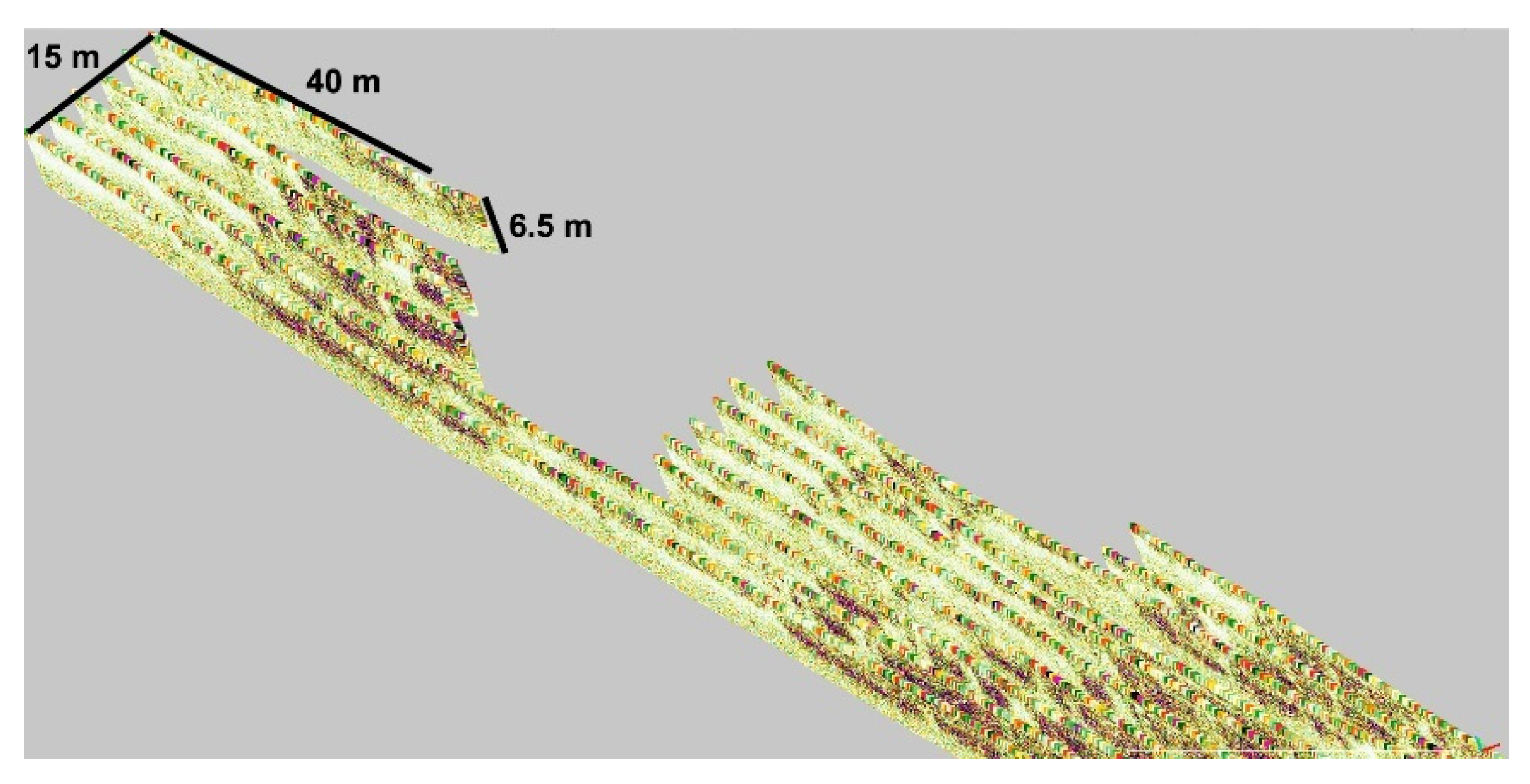
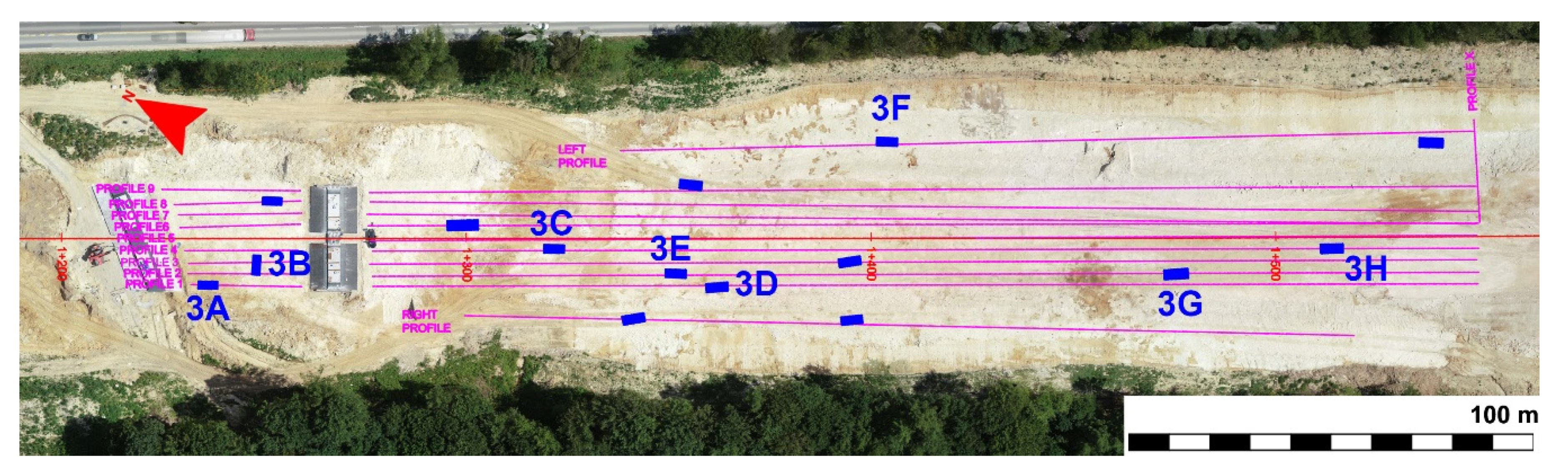
Georeferencing results of GPR data allowed for their integration with the Digital Terrain Model in the form of a point cloud obtained from low-altitude photogrammetric measurements conducted using a UAV. A typical grid of profiling of the research polygons is presented below (Figure 5). The line spacing between adjacent profiles was 3 m, which resulted in an average number of parallel profiles equal to 11. The transverse and diagonal profiles can also be seen in the figure below. Their implementation aimed to assess the geometric compatibility and content repeatability of GPR results at the intersection of profiles with different driving-up directions.

2.3. Methodology of Data Post-Processing

In the case of the GPR method, the extraction of information necessary for correct data analysis required advanced processing algorithms. In the first step, the GPR data was filtered using ReflexW software by Sandmeier & Software. The basic sequence of procedures included:

• Moving the start time to zero as the point of first contact between the electromagnetic wave and the ground;
• Shifting the average signal value to zero—subtract-DC-shift;
• The removal of the low-frequency signal—subtract-mean (dewow);
• The removal of horizontal reflections by the subtraction of average trace—background removal;
• The removal of the bottom part of the radargram without significant reflections—time cut.

The selection of procedures for the second part of the filtering was not accidental but based on years of experience and others’ research [30]. Finally, the following filters were combined in the following processing step:

• Subtracting the average filter.
• Energy Decay as gaining filter.
• Bandpass butterworth filter for band range 50–400 MHz.
• Average xy-filter 3 × 3 for smoothing.
• The filtering procedure resulted in better visibility in the radargrams of regions with variable response characteristics to the electromagnetic field in the medium. However, the analysis of a single vertical B-scan image allowed identifying anomalies or zones of variable parameters but only within the range of a single measurement profile. The full picture of the magnitude of the phenomenon and the variability of the ground nature was observable due to spatial visualization and the integration of GPR and geodetic data.
• Consequently, using the accurate georeferencing of results, GPR radargrams were also converted into the form of an underground radar scanning (UgRS) point cloud. The EM velocity value equals 0.1 m/ns has been used to convert the TWT time into real depth. In contrast to laser scanning measurements, UgRS is based on a recording of the emitted electromagnetic wave amplitude, which carries information about the intensity of the signal reflected from the structures in the ground. The conversion of the time-to-depth value performed based on the propagation wave velocity, allowed us to calculate the full spatial position of the reflection point. The accuracy of the point position was adequate for the measurement method and its geopositioning. GPR data were converted to the UgRS point cloud file based on an original script prepared in MATLAB and ReflexW software. The algorithm consists of two modules that perform the following tasks:
• The conversion of field data into a file format of dedicated software and possible simultaneous coordinates correction [33].
• Processing and saving the filtered GPR radargram in a point cloud file format.

The first procedure concerns Mala’s GPR device and is performed based on data acquired during field measurement, conducted with GPR-GNSS or GPR-robotic total station set. This module is responsible for converting coordinate files, which regards the GPR antenna position as having been recorded using GroundVision software (*.lcg or *.cor file format), to ReflexW software format (*.utm file format). Furthermore, the application allowed the smoothing of the z-coordinate values. This option was particularly important in the case of a positioning solution based on satellite measurements when the precision of the adjacent results is variable. For that purpose, the algorithm used a subtracting average with the possibility of selecting a filter window size. There was also the possibility of a coordinate geometric correction implementation related to the slope of the GPR profile.

The second procedure was based on processed radargrams generated in ReflexW. It allowed the filtered radargram with georeferencing to be written to an ASCII file. The first line of the result file found the total number of points, followed by a stream of xyz coordinates, intensity values (laser beam reflection intensity) and colors in RGB for all points. One advantage of this procedure was the ability to choose whether the traces would be presented as vertical or tilted, according to the surface normal. The slope value was calculated based on the z-values from coordinates in *.utm file.

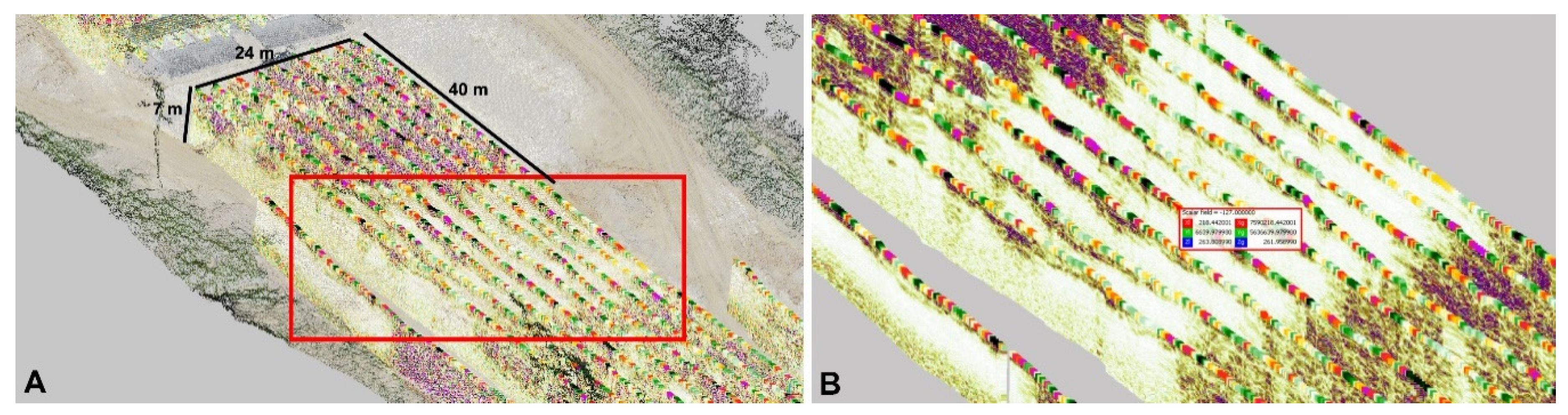
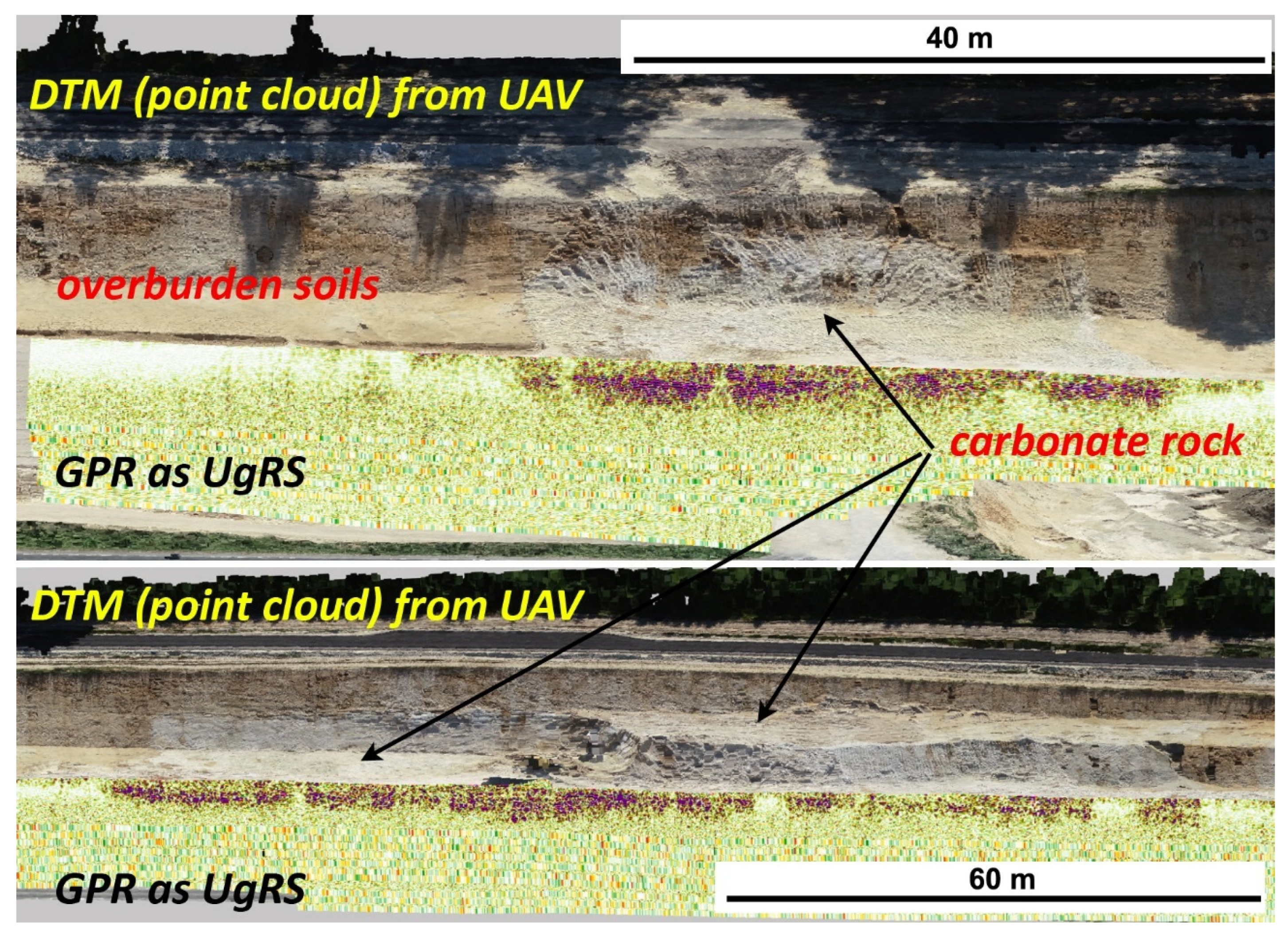
The final result of the process was the ability to handle GPR data as a point cloud and enable their integration with laser-scanning or vector and raster data. The figure below (Figure 6) presents a visualization of the UgRS point cloud with a digital terrain model as a point cloud from one of the research polygons.

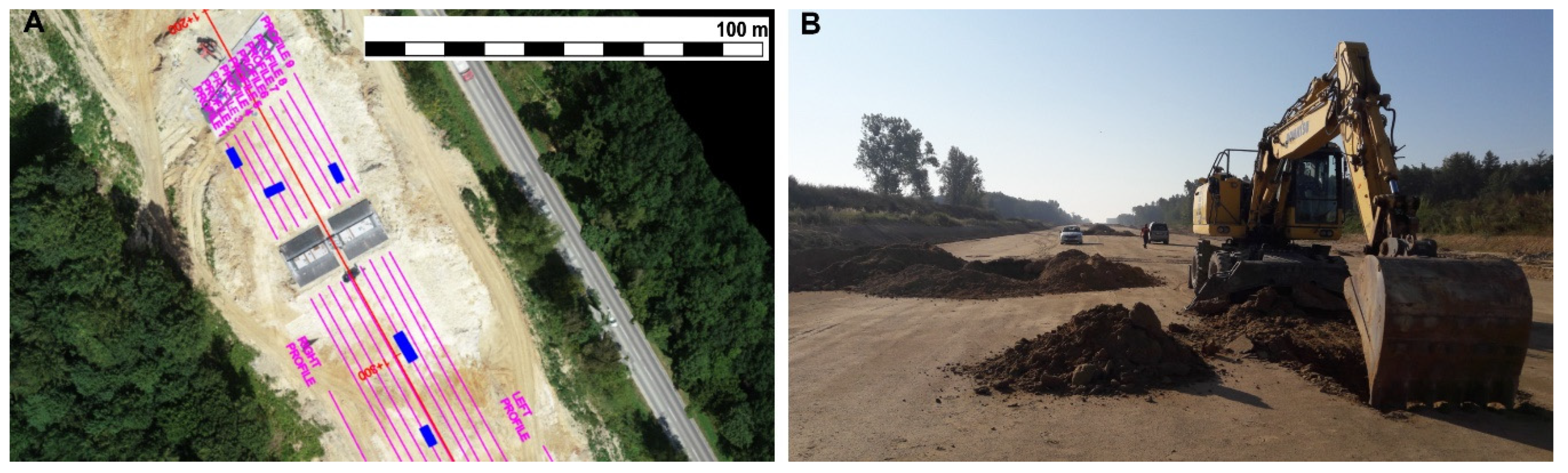
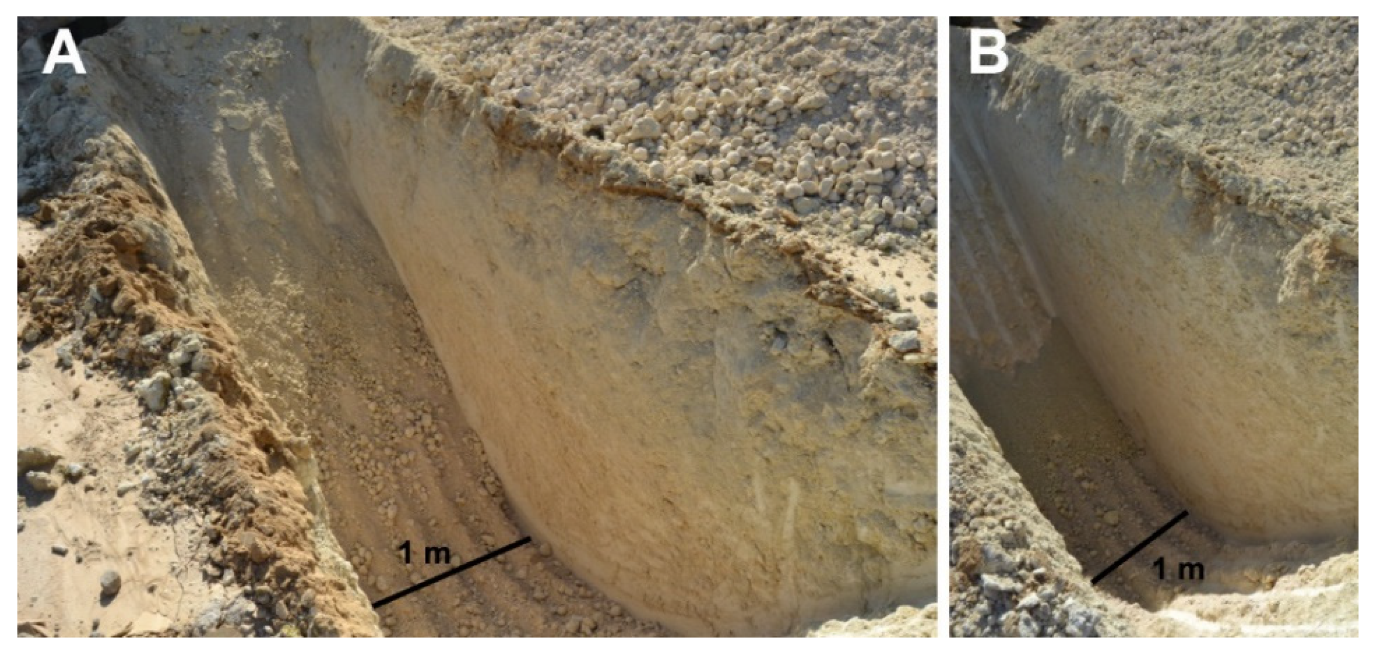
The next crucial step in data processing, which contributed to the increased reliability of the ground variability assessment, was to conduct GPR data calibration. It consisted in comparing selected radargram fragments with corresponding fragments from visible soil structures made possible by, e.g., boreholes and trenches. For this purpose, on the basis of the spatial overview of GPR and DTM data, the accurate locations for a few control trenches were determined on each surface (Figure 7). They were selected so that the confrontation of the real situation with the radargram view would correctly identify potential karst phenomena in the entire research area.

3. Results

Due to the diversified nature of the karst phenomena, the description of the results was divided according to the defined research subregions.

3.1. Polygon 1

This study area included the section where the road planes were formed on a base of native soil for the placement of auxiliary substructure layers (Figure 8). Limestone outcrops were visible between the structure and the slope (light spots on yellow background).

A sample radargram from Polygon 1 with highlighted anomalies is presented in Figure 9. The GPR signal analysis allowed for the distinguishing of zones of enhanced subsurface anomaly occurrence, which are marked by horizontal red lines. These zones have several types of identified anomalies, depending on their signal reflection: for anomalies A1 and A2, this was from the surface to the medium; A3 anomalies were shallow below the surface; A4 anomalies were clearly below the surface; and significant anomalies included those marked A5—more or less shallow, but which strongly reflected the radar signal. From the point of view of a void search, anomalies of type A4, A3 and A5 were extremely important and required direct verification to determine their real nature.

The application of GPR data conversion to a UgRS point cloud allowed for the spatial analysis of GPR imaging and confrontation with exposed zones of the road corridor. A significant positive signal distribution correlation with intersecting transverse, longitudinal and diagonal profiles was especially visible due to the spatial arrangement of the radargrams (Figure 10).

The identification of two zones is particularly straightforward in the spatial visualization of radargrams: intense anomalies with a diversified layout zone and a strong attenuation zone (Figure 11A). The relationship between the DTM and UgRS point clouds is presented in Figure 11B. It should be noticed that the strong reflections in the central part of the area correlated well with the limestone outcrops, which are continued on the left side of the image.

In the area of Polygon 1, several direct exposures of a 1 × 4 m, cone-shaped trench were created, up to a depth of 3–3.5 m. As an example, 3 out of 7 selected pits were presented in more detail. The first trench, 1A, was carried out in the zone of strong reflections. It clearly showed that the anomalies at a depth of 1 m (99 m of the profile) correlated with the ceiling of the limestone layers discovered in the trench, which are soft and clayey (Figure 12). In the case of the next exposure, 1B, (289 m of profile) in the upper soil layer, a completely different signal response was recorded. It had a shoal arrangement—a tight cluster that correlated with a crumbling, very fine dusty material (Figure 13). Below the ordered layer, a less regular signal appeared, which correlated with the limestone rock and confirmed the conclusion of the previous outcrop. The last trench, 1C, (145 m of the profile), occurring in the area of the visible rock outcrop, confirmed the spatial continuation of this geological structure (Figure 14). Of special note was the nature of the rock, which was different compared to previous exposures. Although the limestone formations did not stand out so clearly from the background; they had a different appearance. The rock was still brittle but more compact, with a different resistance on the excavator bucket.

3.2. Polygon 2

In the area of Polygon 2, GPR measurements were conducted after the road corridor was prepared, mostly on the surface of the native soil. Only the first part of the profiles, about 20 m long, was measured along with a thin layer of material included in the road base (Figure 15, gray color).

Analysis of GPR results in the form of vertical B-scan radargrams and a UgRS point cloud revealed a significant positive correlation between the occurrence of carbonate rock zones and GPR signal response. The phenomenon was well illustrated by the combination of geodetic and GPR data displayed in the side view. The radargram presented a strong attenuation and lack of GPR signal reflections in the area of overburdened soil, the opposite reaction to the concentration of clear signal responses in the area of carbonate rock (Figure 16).

Zones with the varied intensity of strong GPR signal reflections were observed in the study area. However, during field inspections, no caverns or areas of visible fractures or ground loosening were identified (Figure 17).

The exposures performed in the areas of increased anomaly density mainly indicated the variability of the rock fractions and the degree of the material compaction, and the results of 3 are presented.

Trench 2A at 50.5 m of profile 12 showed the presence of granular carbonate rock in the upper soil layer. Below this, at a depth of about 0.7 m, we entered a zone of compacted granular material (Figure 18). The other trenches in this region revealed a similar soil nature. The next exposure, 2B (Figure 19), located in the zone of higher signal attenuation, confirmed the correlation between the recorded radargram and the occurrence of re-filled karst funnels. The deeper trough exposed carbonate rock with small, compact granulation. The last exposure, 2C, in an area of poor signal response in the GPR image, correlated with carbonate rock with a granular but homogenous and compact form (Figure 20).

Most of the results from the trenches, with the exception of a few highly attenuated places, confirmed that the signal reflection intensity was strongly related to the variability of the limestone rock fraction, which seemed to occur at the confluence of strongly blended variable carbonate structures. However, it was not possible to systematize the variation of the signal according to the condition of the rock.

3.3. Polygon 3

Karst phenomena detected during road works in the area of polygon 3 required additional GPR measurements even though road construction was already in progress. The figures below present a few examples of the infiltration into carbonate rocks of karst phenomena and forms re-filled with clay–sandy material. Of particular concern was the rainwater dripstone identified on the exposed slopes (Figure 21).

The analysis of available ALS cartographic materials for Polygon 3, collected in national geoportals, indicated the presence of karst funnels, which are intensively concentrated in the near surroundings of the investment area (Figure 22).

Furthermore, ALS data allowed for the observation of significant ground height differences in the study area, which affected the formation of gullies for periodic streams. The whole area of Polygon 3 was characterized by intense differentiation of the subsoil on a section of about 500 m, which was well illustrated on the UgRS point cloud (Figure 23).

Fractures were also found on the ground surface in this area (Figure 24) and were especially visible beyond the crown of the road construction. Therefore, additional GPR measurements were performed outside the regular grid of profiles marked in Figure 25 as the right and left additional profiles.

A sketch of the trench location for Polygon 3 is presented below (Figure 25).

The photos of exposures 3A performed in Polygon 3 clearly showed a limestone outcrop with visible flow tracks and a clay overburden, which unambiguously correlated with the intensity of the recorded GPR signal (Figure 26, on 4.9–10.0 m of the profile). In the case of trench 3B, strong signal responses with high amplitude correlated with the structure of the limestone rock. This exposure was carried out on a profile, where between 15.0 and 20.0 m signal amplitude length values were very high and strongly concentrated from the very top of the radargram. Only a very shallow trough was created due to the high resistance of the rock on the excavator bucket, which was sliding as if on solid rock (Figure 27).

Another significant exposure, 3C, was located in the gully zone due to the variability of the imaging of the ALS data observed in the top view (clay zone, brown color of the ALS point cloud). The trench was carried out on 44.8 m of the GPR profile. Photographs of the trench showed a small overburden of limestone with formations underneath. It is possible that the weak reflections on the radargram at a depth of 2.5 m were the result of outcrop exposure (Figure 28). It also correlated with the ALS image, where the ground on the west side of the trough changed to a bright color, just like carbonate rock.

The location of the last of the 3D exposures for Polygon 2 was selected in areas of local GPR signal attenuation and correlated well with the zones of karst funnels refilled with clay. It could be seen that the clay overburden in the trench revealed strongly attenuated the signal. Although the funnel ended, the continuation of the rock floor was weakly visible on the radargram. The photographs show horizontal cracks (Figure 29), also revealed in several other trenches (3E, 3F). The cracks expired below a depth of 3.5–4 m of exposure. However, the edge line of the fissures was new and aligned perpendicular to the terrain fall line. Considering the relief of the rock mass and the fact that the elevation of the terrain strongly decreased in the longitudinal direction to the road, the reasons for the revealed cracks had to be found in the construction activities and terrain elevation transformations.

3.4. Polygon 4

GPR surveys in the area of Polygon 4 covered a section of the already completed road surface. Conducting the measurements was necessary because the character of the ground in the road corridor corresponded to that of Polygon 3, and the contractor assured that the supporting substructure layers were made of material with slag elements. Based on previous experience with strong signal attenuation in such layers, it was decided to perform GPR profiles both on the finished road structure and beyond the technical road. The purpose of these measurements was to demonstrate the limitation of the non-destructive GPR method for identifying karst phenomena on already constructed road sections. The trajectories of both profiles were designed to be very close to each other (Figure 30).

Figure 31 presents the geological character of the area. The GPR survey along the profile beyond the road construction was continued along the slope, which was crucial because the native soil was not affected; therefore, the measurements accurately represented the reaction of the GPR signal to the existing overburden formations above the limestone layer.

The comparison of radargrams acquired on both profiles clearly confirmed the strong attenuation of the radar signal in already completed road surface structures (Figure 32). These results showed a significant relationship between the signal response and the limestone outcrops revealed in the technical road.

The profile was conducted on the native soil surface, so the slope of the road (Figure 33) required an additional interpretation (Figure 33, up to 220 m of the profile). In the radargram at a depth of 3–4 m, clear anomalies connected with the crossing from the clay layer to the carbonate rock were visible. Particular attention was paid to anomalies below 7-m deep and up to 120 m along the profile. It was difficult to determine the genesis of this phenomenon but the ability to record a GPR signal response at such a depth was very important. The measurement results indicated that the geophysical application methods certainly provided a view of soil variability and allowed for a better selection of drilling points.

These conclusions were confirmed through the exposures. In the case of Trench 4A, performed on 199 m of the profile, the GPR signal on the radargram corresponded very well with the situation in the field. In the area where there were strong reflections on the image, an outcrop of carbonate rock became visible (Figure 34). The further exposure 4B was also made in the area of a strong signal response, identified as between 200 and 280 m of the profile. In these places, the excavated rock material was tough with a lumped fraction (Figure 35). However, Trenches 4C and 4D on 321 and 391 m of the profile, respectively, presented a different limestone rock character: compact, when the rock was still in the trench. and loose with a fine fraction after excavation (Figure 36). This phenomenon was reflected in the different character of the GPR signal because the number of strong reflections decreased.

3.5. Polygon 5

Polygon 5 (Figure 37) was located about 4 km from the others previously described; however, it retained the correlations between GPR signal intensity and the occurrence of carbonate rock zones and clay–sandy overburden discussed in the earlier fields.

Additionally, the relationship between the rock structure and the intensity and amplitude concentration of the GPR signal response was considered. Figure 38 presents the DTM and UgRS of the area from various perspectives and directions of observation. The bottom view is significant because the relationship between DTM and UgRS information is perfectly illustrated in the case of longitudinal and transverse profiles. The mutual correlation of the intersecting UgRS is also remarkable.

4. Discussion

The purpose of this study was to present the methodology of conducting and analyzing GPR surveys on selected parts of a newly built expressway to determine the interpretation keys for identifying the location of karst forms such as sinkholes or karst funnels.

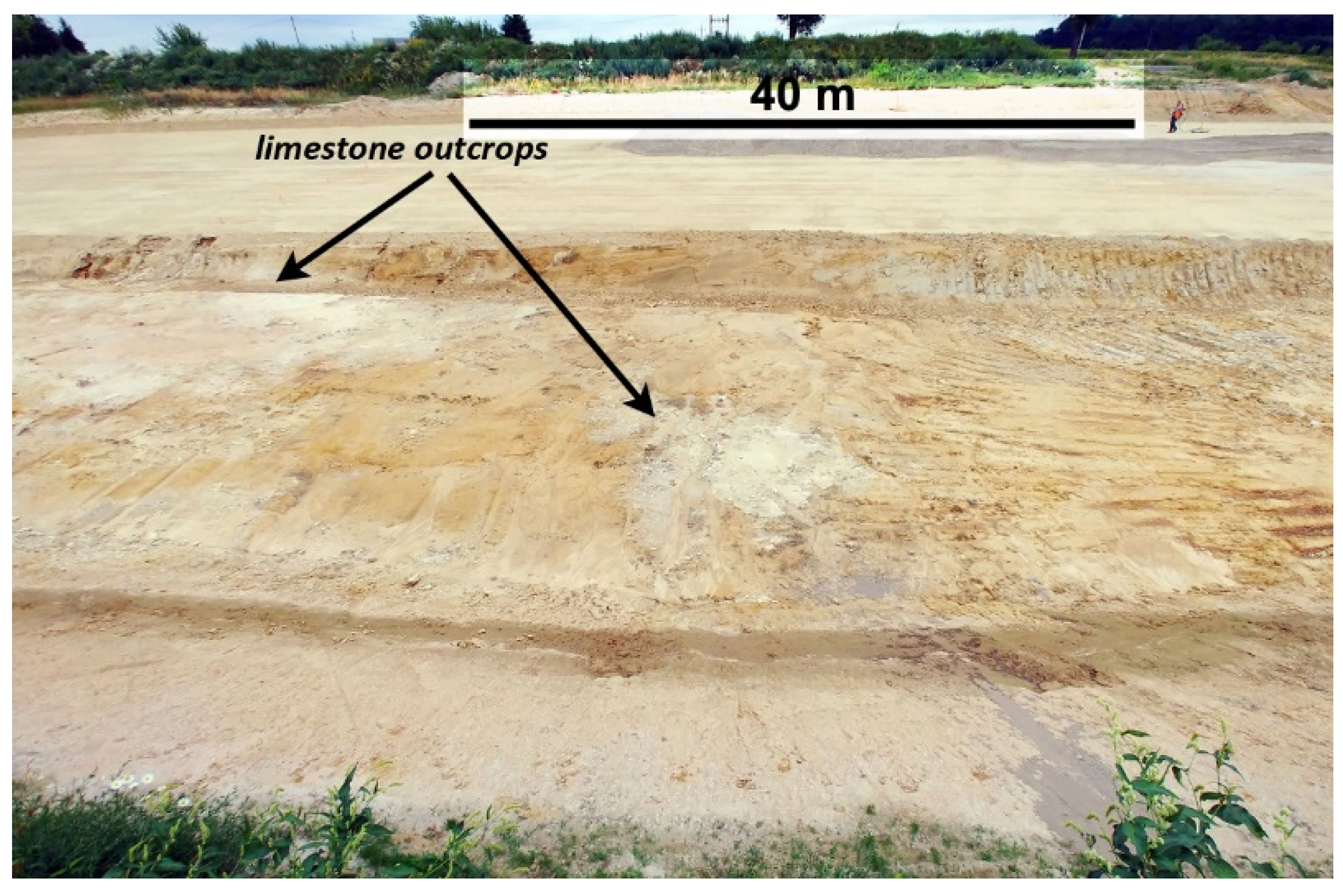
The work was conducted under specific conditions while the construction of the project was in progress. The measurement area mostly covered the road section levelled to the road alignment. The distribution and intensity of the carbonate rocks and overburdened materials were evident in the exposed soil regions. Carbonate outcrops dominated; hence, in accordance with the mentioned “Guidelines”, the ERT method was excluded in favor of GPR. Furthermore, as presented in Figure 1, GPR also allowed the identification of subsurface voids, which would have been challenging for the ERT method.

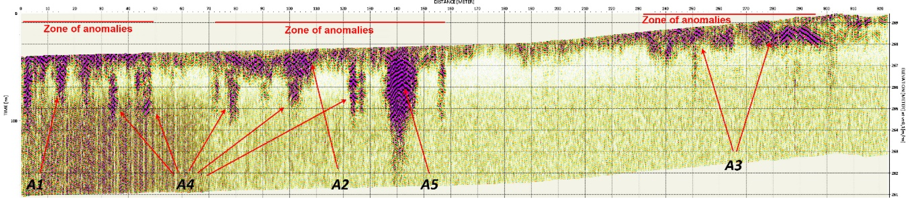
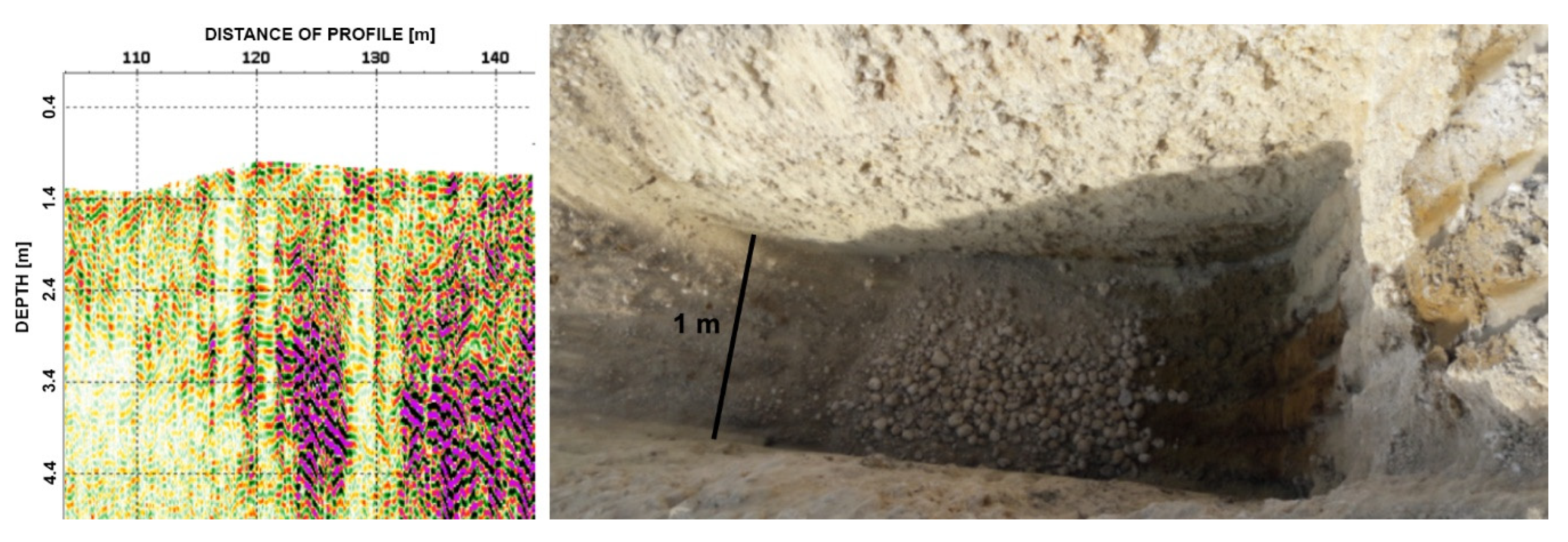
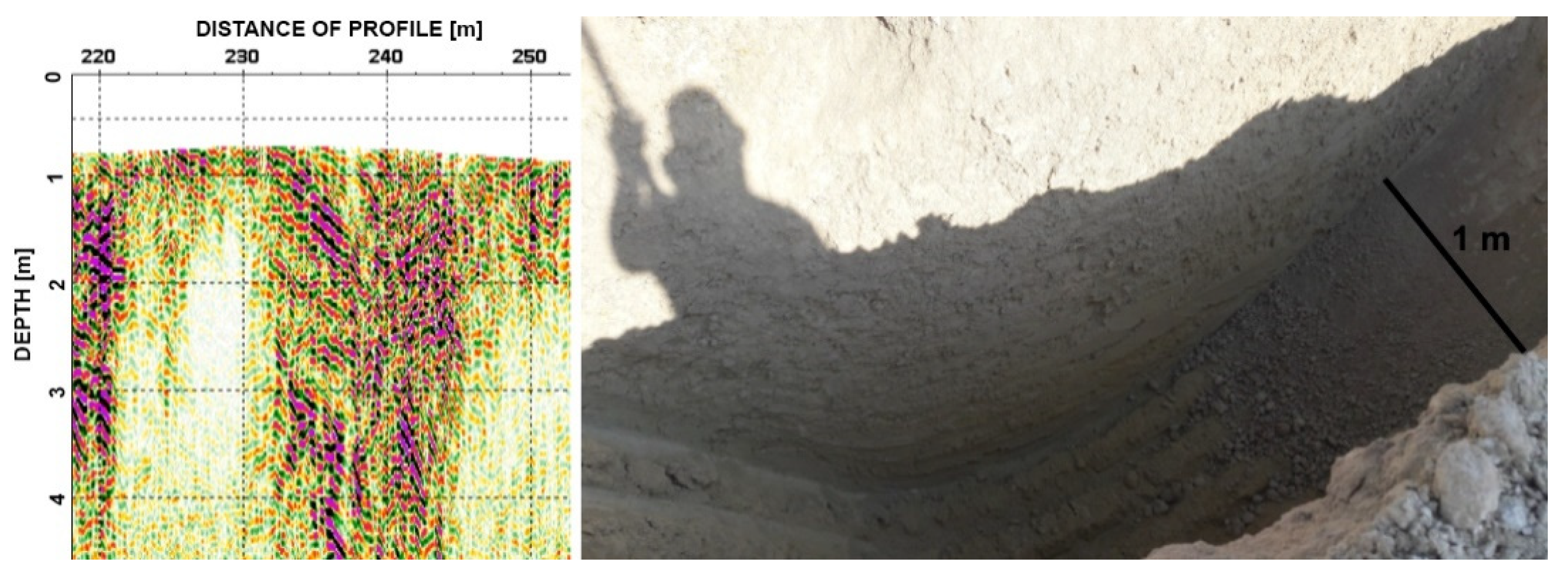
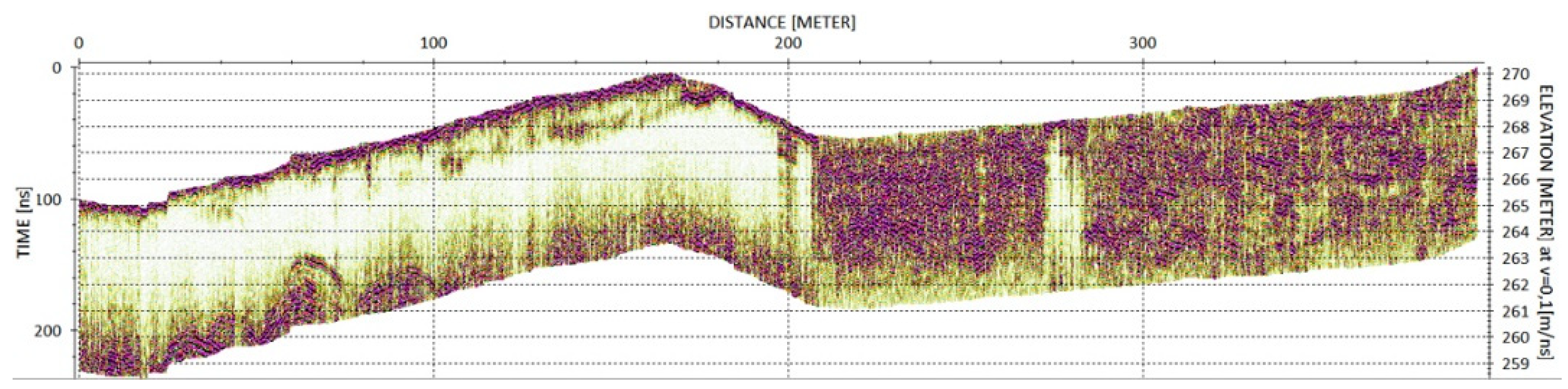
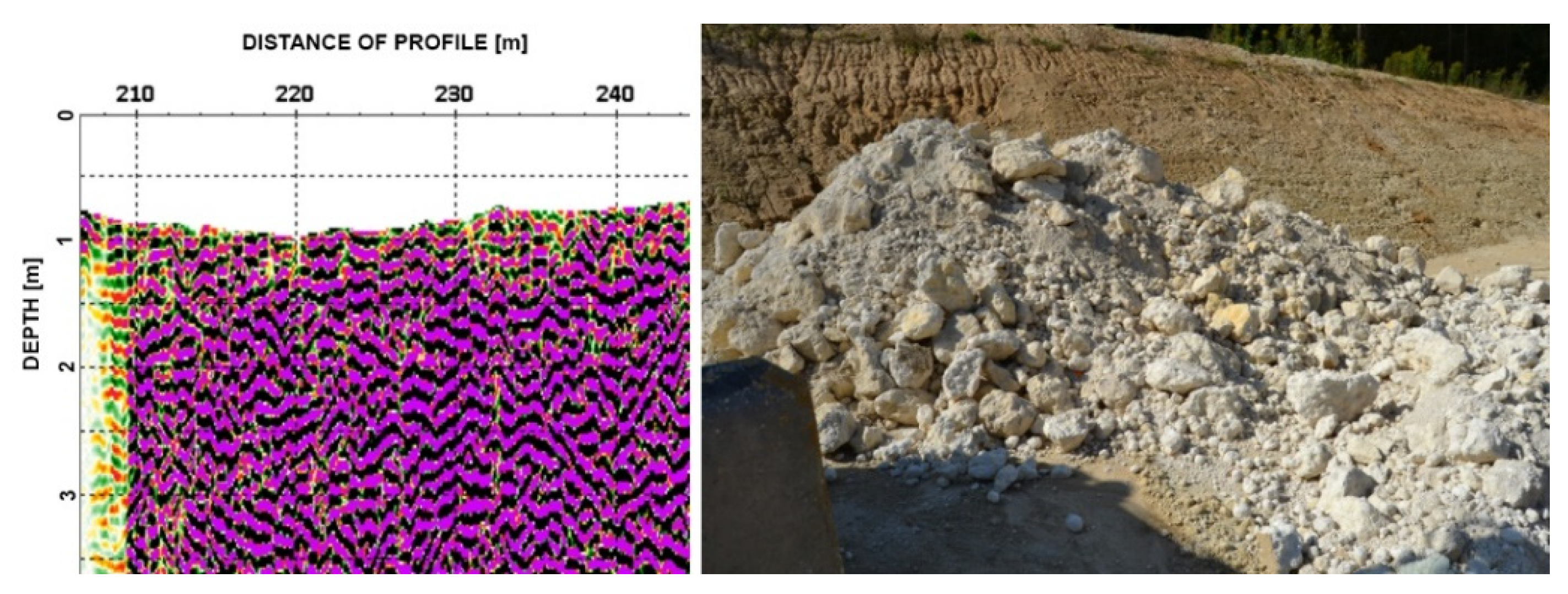
In the examples, despite the use of an antenna frequency of 250 MHz, which was a compromise between the measurement resolution and the expected range of effective penetration, the layer boundaries with large differences in relative electric permeability were very clearly mapped on radargrams. The analyzed fragments showed that the soil variability, even including the variability of the carbonate rocks, themselves (compact/fine/loose/aggregate), correlated with the distribution of signal variability in the GPR radargrams. In places where strong reflections appeared, the rock was compact. The GPR response lost strength in the areas of loosened or weathered rock. Completely weak signals indicated a correlation with areas of overburden with clay or clay–sandy material, including karst funnels refilled with clay material.

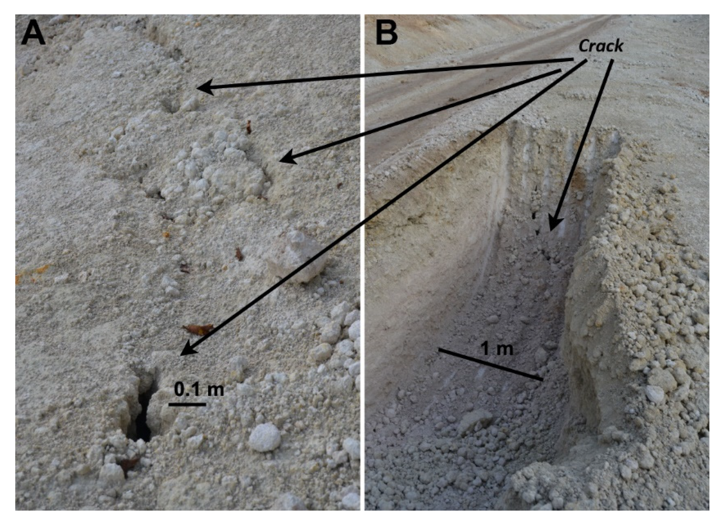
However, it should be highlighted that an accurate determination of the nature of the observed soil variability was not possible because only GPR data were available. The remote sensing nature of the method is naturally associated with a significant uncertainty of identification and forces the development of interpretation keys through direct measurements in trenches. Strong reflections on radargrams may have indicated a void as well as a rock with crumbly nature. Hence, it was necessary to compare the GPR material with the exposed ground fragments. To categorize the type of soil over large areas even roughly, it was necessary to assume the homogeneity of the identified anomalies throughout the study area. Additionally, the physical principles of the GPR method made some phenomena impossible to identify. This was confirmed by the example of the ineffectiveness of identifying a few fractures in trenches up to a depth of 3 m. Despite using an antenna with a high frequency of 700 MHz, the cracks were too small for their boundaries to be determined on the radargram among the signal responses from crumbly heterogeneous rock.

An important aspect supporting ground recognition in GPR data analysis is the novel approach to their visualization.

For a long time, the integration of GPR and geodetic data focused on the method and geolocation of radargrams and their assessment [34,35,36]. The ability to precisely determine the position of GPR data allowed for the implementation of further steps, i.e., combining the GPR data with the results of other sensors and derived products, especially rasters, such as orthophoto or DTM. In many cases, GPR data, through interpolation algorithms, were transformed to cube form, which allowed for the generation of horizontal cross-sections–C scan. This approach is effective for anthropogenic objects that exhibit a certain regularity of form in a spatial system [37,38]. However, it limits the analysis to a simultaneous view of a single cross-section at a predetermined depth or inclined plane, which significantly affects the possibility of full spatial interpretation of the results. The approach presented in our work is based on GPR data visualization as an UgRS point cloud. It avoids the problem of limited possibilities of correct interpolation of irregular shapes of natural objects. The data is still presented spatially, but without the redundancy of artificial interpolation data.

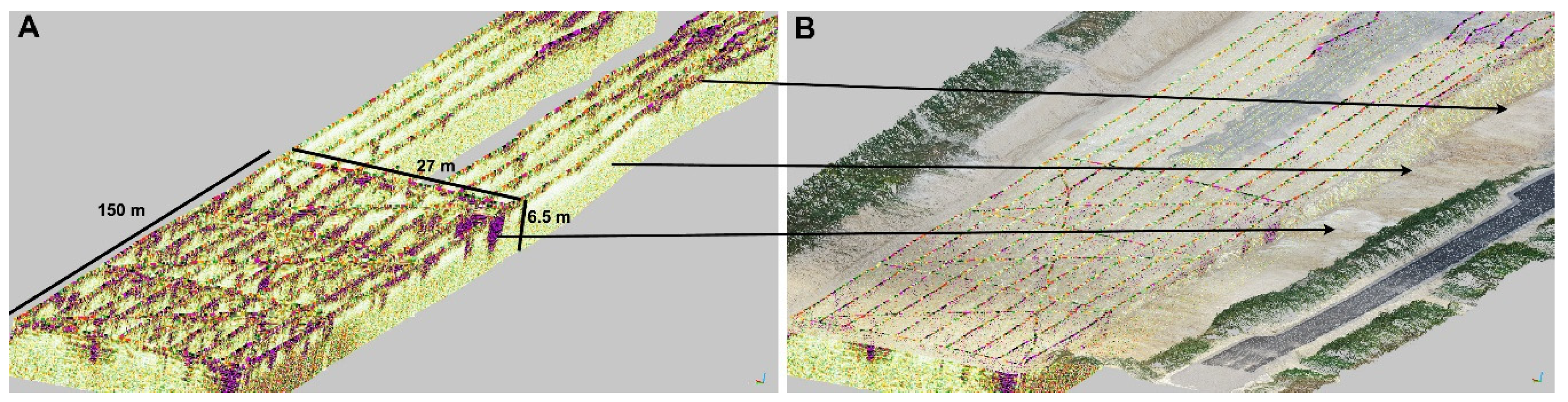
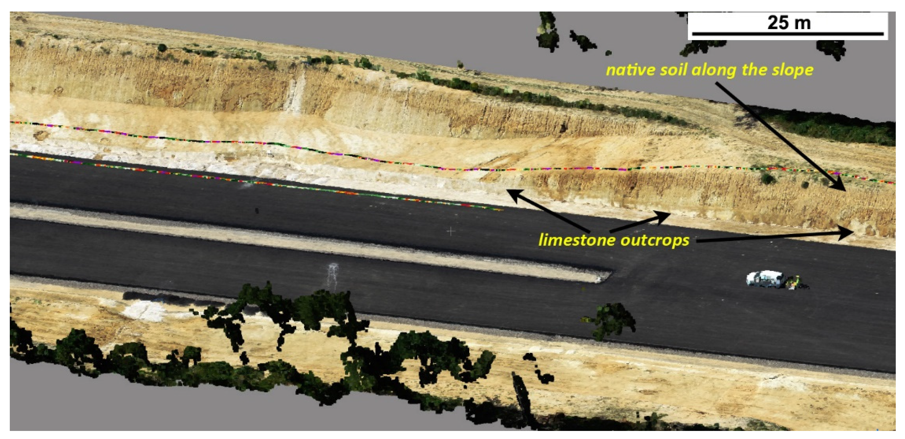
Furthermore, due to the accurate geolocation and radargram conversions using the author’s algorithm, it was possible to spatially compile the GPR and geodetic data in software specific to 3D object analysis. The spatial combination of the results of these remote sensing methods in one visualization made it possible to identify the correlation between the ground surface, visible on the DTM data in the point cloud form, and the recorded GPR data. In particular, a strong relationship was identified between areas of clay–sandy soil or visible limestone outcrops and the distribution of GPR signal amplitude on radargrams, which showed strong attenuation.

The essence of the joint data presentation in the form of a point cloud and supporting the analysis of the subsurface situation through the premises observed on the surface data strengthens the quality and interpretational credibility, which is emphasized in the publication [39]. An additional value of the spatial analysis of UgRS data was the possibility of assessing the consistency of radargram content distribution on intersecting profiles, as in the case of Polygon 1. High coherence in the arrangement of signal-response amplitudes proved both the high relative accuracy of the GPR data location as well as their non-random local character. Thus, it increased the reliability of the method as stable and repeatable. The integration of DTM and UgRS point clouds also enabled the efficient and unambiguous selection of optimal sites for control trenches. The analysis of the material focused on those fragments of the GPR data that represented areas of an anomaly with the compact and strong amplitude of the back signal. However, while the nature of the GPR signal response in some fragments of the study areas did not clearly indicate the presence of large voids, the amplitude analysis in the surface approach indicated a small void in the crack networks of the rock material, which significantly affected ground load-bearing capacity. This was a serious indication for the execution of a control trench in this place.

Unfortunately, no soil samples were collected during the work, and thus it was not possible to determine the variability of ground structure and composition in the road laboratory. Ground analysis performed in this way could lead to enhanced calibration of radargrams and the determination of precise interpretation keys in a numerical approach. This would allow for the automation or semi-automation of the classification of the nature of soil changes, including even a quantitative assessment of anomaly distribution in the surveyed area. This assessment for Polygon 3 is as follows:

• Characteristics revealed in the trenches 3A, 3B covered 20% of the surveyed area
• In trench 3C it was about 9%
• In trench 3D, about 47%
• In trenches 3G and 3H, 10%.
• An embankment covers about 7% of the area.
• Minor local areas of strong attenuation cover about 6% of the area.

It was also concluded that with a large base of accurate interpretation keys, automation of ground classification would reduce the necessity of assuming a homogeneous nature of change within a whole study area.

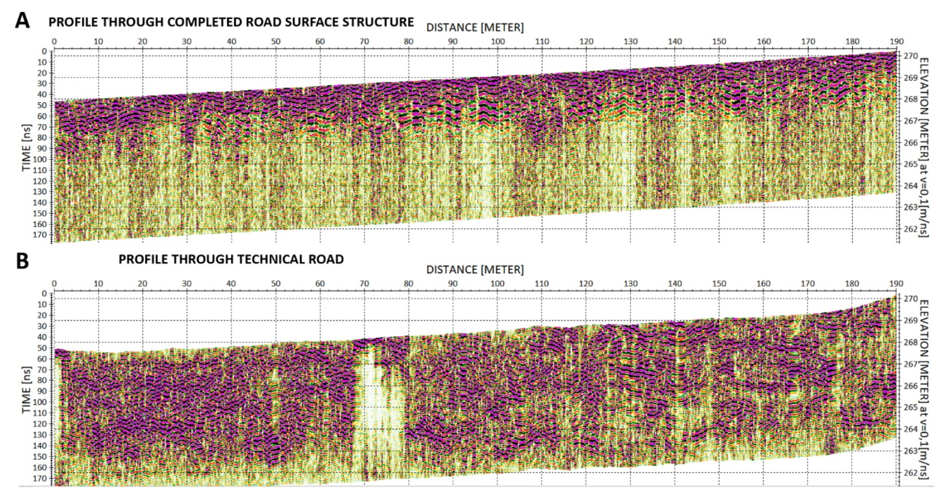
The necessity of conducting complementary research resulting from the discrepancy between the existing geological materials and the actual state in the field only highlights the importance of correct soil recognition, as early as the design stage, both for infrastructural and cubature investment. As our research showed, it resulted not only in a safety issue and reduced additional costs, but also a much lower possibility of effective identification when construction is at an advanced level. Where GPR measurement was carried out on a road surface under which slag material was located, only a strong attenuation of the signal was visible on the radargram. Thus, it was concluded that the implementation of non-destructive geophysical surveys should occur at the latest before the formation of such a layer. The demonstration of this relation by comparison with the respective radargrams (Figure 32) had a broader meaning. If the survey aim were to conduct subsoil recognition for an existing road modernization, and there were indications that the supporting substructure layer included slag, limitations can be expected from the very beginning.

5. Conclusions

The “Guidelines” systematize and introduce a clear methodology for conducting geophysical surveys and classifying the cases of their application.

GPR research should be performed before conducting invasive tests so that they can be targeted at areas of identified anomalies or variations in signal behavior. It was possible to conduct GPR measurements during investment construction to obtain additional information after removing the layers to the level of the road alignment but before laying the structure layers with slag elements. Carrying out a survey on a completed road structure with the presence of such a layer strongly reduced the effectiveness of the GPR method. This should be carefully considered when planning the work. In some cases, measurements should be designed outside the roadbed if possible due to site accessibility.

Requiring the geopositioning of GPR measurements had positive consequences in processing and interpreting the GPR data. First of all, it enabled the implementation of the proposed methodology by converting radargrams into a UgRS point cloud. This was an original approach, which as presented in the publication in combination with DTM data, gave an improved interpretation and understanding of GPR–substrate relations.

This practical example, which implemented GPR, demonstrated that we can all conduct a full and efficient integration of remote sensing data from various sources. The digitization of the construction process seems to be an irreversible trend. In addition, the example confirmed the high effectiveness and usefulness of using the GPR method to identify the variability of the substrate, especially in areas of carbonate rocks where karst phenomena and forms may occur.

References

1. Dec, J. High resolution seismic investigations for the determination of water flow directions during sulphur deposits exploitation. Acta Geophys. 2010, 58, 5–14. [Google Scholar] [CrossRef]
2. Holmes, J.; Chambers, J.; Meldrum, P.; Wilkinson, P.; Boyd, J.; Williamson, P.; Huntley, D.; Sattler, K.; Elwood, D.; Sivakumar, V.; et al. Four-dimensional electrical resistivity tomography for continuous, near-real-time monitoring of a landslide affecting transport infrastructure in British Columbia, Canada. Near Surf. Geophys. 2020, 18, 337–351. [Google Scholar] [CrossRef] [Green Version]
3. Stěpančíkova, P.; Dohnal, J.; Pánek, T.; Łój, M.; Smolková, V.; Šilhán, K. The application of electrical resistivity tomography and gravimetric survey as useful tools in an active tectonics study of the Sudetic Marginal Fault (Bohemian Massif, central Europe). J. Appl. Geophys. 2011, 74, 69–80. [Google Scholar] [CrossRef]
4. Czarniak, P.; Pacanowski, G.; Sobótka, P. Zastosowanie badań konduktometrycznych z uzyciem inwersji ID, jako narzȩdzia do kartowania przestrzennego przypowierzchniowych warstw geologicznych. Przegląd Geol. 2017, 65, 803–810. [Google Scholar]
5. Vanella, D.; Ramírez-Cuesta, J.M.; Intrigliolo, D.S.; Consoli, S. Combining electrical resistivity tomography and satellite images for improving evapotranspiration estimates of citrus orchards. Remote Sens. 2019, 11, 373. [Google Scholar] [CrossRef] [Green Version]
6. Zieliński, A.; Mazurkiewicz, E.; Łyskowski, M. Kartiranje krških formacija ispod povijesne zgrade u Szydłówu u Poljskoj pomoću georadara. Geofizika 2016, 33, 101–111. [Google Scholar] [CrossRef]
7. Cheng, Q.; Tao, M.; Chen, X.; Binley, A. Evaluation of electrical resistivity tomography (ERT) for mapping the soil–rock interface in karstic environments. Environ. Earth Sci. 2019, 78, 1–14. [Google Scholar] [CrossRef] [Green Version]
8. Sokołowska, M.; Chada, M.; Roguski, A.; Majer, E. Ocena badań geologiczno-inzynierskich wykonanych na potrzeby inwestycji drogowych w latach 2007–2016. Przegląd Geol. 2017, 65, 672–677. [Google Scholar]
9. Borecka, A.; Ostrowski, S. Analiza obowiązujących przepisów prawnych w zakresie stosowania metod geofizyki inzynierskiej. Przegląd Geol. 2017, 65, 678–684. [Google Scholar]
10. Reynolds, J.M. An Introduction To Applied Geophysics; Wiley & Sons: New York, NY, USA, 1997. [Google Scholar]
11. Van Der Merwe, A.; Gupta, I.J. A Novel signal processing technique for clutter reduction in gpr measurements of small, shallow land mines. IEEE Trans. Geosci. Remote Sens. 2000, 38, 2627–2637. [Google Scholar] [CrossRef] [Green Version]
12. Greco, M.S.; De Maio, A. (Eds.) Modern Radar Detection Theory; IET: London, UK, 2015; Volume 2. [Google Scholar]
13. Rajchel, B. Ocena zastosowania georadaru do wykrywania podziemnych instalacji budowlanych w warunkach zimowych. Przegląd Geol. 2017, 65, 790–795. [Google Scholar]
14. Šarlah, N.; Podobnikar, T.; Mongus, D.; Ambrožič, T.; Mušič, B. Kinematic GPR-TPS model for infrastructure asset identification with high 3D georeference accuracy developed in a real urban test field. Remote Sens. 2019, 11, 1457. [Google Scholar] [CrossRef] [Green Version]
15. Feng, D.; Wang, X.; Zhang, B. Specific evaluation of tunnel lining multi-defects by all-refined GPR simulation method using hybrid algorithm of FETD and FDTD. Constr. Build. Mater. 2018, 185, 220–229. [Google Scholar] [CrossRef]
16. Łyczak, M.; Adamiec, J.; Skupień, T.; Małysa, T.; Groffik, A. Georadar surveys of the flooring in the St. Francis of Assisi basilica in Krakow. Geol. Geophys. Environ. 2018, 44, 357. [Google Scholar] [CrossRef]
17. Skolnik, M.I. Chapter 21 Ground Penetrating Radar. In Radar Handbook, 3rd ed.; The McGraw-Hill Companies: New York, NY, USA, 2008. [Google Scholar]
18. Beres, M.; Luetscher, M.; Olivier, R. Integration of ground-penetrating radar and microgravimetric methods to map shallow caves. J. Appl. Geophys. 2001, 46, 249–262. [Google Scholar] [CrossRef]
19. Pavlič, M.U.; Praznik, B. Detecting karstic zones during highway construction using ground-penetrating radar. Acta Geotech. Slov. 2011, 8, 17–27. [Google Scholar]
20. Gosar, A. Analysis of the capabilities of low frequency ground penetrating radar for cavities detection in rough terrain conditions: The case of Divača cave, Slovenia. Acta Carsologica 2012, 41, 77–88. [Google Scholar] [CrossRef]
21. Karczewski, J.; Ortyl, Ł.; Pasternak, M. Zarys Metody Georadarowej, 2nd ed.; Wydawnictwa AGH: Kraków, Poland, 2011. [Google Scholar]
22. Busetti, A.; Calligaris, C.; Forte, E.; Areggi, G.; Mocnik, A.; Zini, L. Non-Invasive Methodological Approach to Detect and Characterize High-Risk Sinkholes in Urban Cover Evaporite Karst: Integrated Reflection Seismics, PS-InSAR, Leveling, 3D-GPR and Ancillary Data. A NE Italian Case Study. Remote Sens. 2020, 12, 3814. [Google Scholar] [CrossRef]
23. Weight, W.D. Chapter 4 Basic Geophysics of the Shallow Subsurface. In Manual of Applied Field Hydrogeology; The McGraw-Hill Companies: New York, NY, USA, 2001. [Google Scholar]
24. Popiołek, E.; Pilecki, Z. (Eds.) Ocena Przydatności do Zabudowy Terenów Zagrożonych Deformacjami Nieciągłymi za Pomocą Metod Geofizycznych; Wydawnictwo IGSMiE PAN: Kraków, Poland, 2008. [Google Scholar]
25. Madej, J.; Łój, M.; Porzucek, S.; Jaśkowski, W.; Karczewski, J.; Tomecka-Suchoń, S. The geophysical truth about the ‘Gold Train’ in Walbrzych, Poland. Archaeol. Prospect. 2018, 25, 137–146. [Google Scholar] [CrossRef]
26. Żuk, T.; Smith, G.H.S. Stratygrafia radarowa–metoda analizy danych georadarowych 3D w badaniu środowisk sedymentacyjnych na przykładzie osadów rzecznych. Przegląd Geogr. 2015, 87, 439–456. [Google Scholar] [CrossRef]
27. Su, M.; Zhao, Y.; Xue, Y.; Wang, P.; Xia, T.; Zhang, K.; Li, C. Progressive Fine Integrated Geophysical Method for Karst Detection During Subway Construction. Pure Appl. Geophys. 2021, 178, 91–106. [Google Scholar] [CrossRef]
28. Ba, X.; Li, L.; Wang, J.; Zhang, W.; Fang, Z.; Sun, S.; Liu, Z.; Xiong, Y. Near-surface site investigation and imaging of karst cave using comprehensive geophysical and laser scanning: A case study in Shandong, China. Environ. Earth Sci. 2020, 79, 298. [Google Scholar] [CrossRef]
29. Bermejo, L.; Ortega, A.I.; Parés, J.M.; Campaña, I.; Bermúdez de Castro, J.M.; Carbonell, E.; Conyers, L.B. Karst features interpretation using ground-penetrating radar: A case study from the Sierra de Atapuerca, Spain. Geomorphology 2020, 367, 107311. [Google Scholar] [CrossRef]
30. Ortyl, Ł. Geometrization of karst phenomena based on GPR research. Przegląd Geol. 2019, 67, 252–269. [Google Scholar] [CrossRef]
31. Dobrowolski, R.; Harasimiuk, M.; Brzezińska-Wójcik, T. Strukturalne uwarunkowania rzeźby Wyżyny Lubelskiej i Roztocza. Przegląd Geol. 2014, 62, 51–56. [Google Scholar]
32. Szrek, D.; Kwecko, P.; Miecznik, J.; Wojtyna, H.; Wojciechowska, K. Objaśnienia do Mapy Geośrodowiskowej Polski 1:5000. Arkusz Janów Lubelski; Centralne Archiwum Geologiczne PIG-PIB: Warszawa, Poland, 2011. [Google Scholar]
33. Ortyl, Ł.; Owerko, T. Korekta wpływu deniwelacji terenu oraz częstotliwości wyznaczenia pozycji przez system GNSS lub tachymetry TCA w procesie przestrzennej lokalizacji obiektów wykrywanych georadarem. Zesz. Nauk. Górnictwo/Politech. Śląska 2007, 278, 335–352. [Google Scholar]
34. Lehmann, F.; Green, A.G. Semiautomated georadar data acquisition in three dimensions. Geophysics 1999, 64, 719–731. [Google Scholar] [CrossRef]
35. Grasmueck, M.; Viggiano, D.A. Integration of ground-penetrating radar and laser position sensors for real-time 3-D data fusion. IEEE Trans. Geosci. Remote Sens. 2007, 45, 130–137. [Google Scholar] [CrossRef]
36. Kutuzov, S.; Thompson, L.G.; Lavrentiev, I.; Tian, L. Ice thickness measurements of Guliya ice cap, western Kunlun Mountains (Tibetan Plateau), China. J. Glaciol. 2018, 64, 977–989. [Google Scholar] [CrossRef] [Green Version]
37. Gaballah, M.; Grasmueck, M.; Sato, M. Characterizing Subsurface Archaeological Structures with Full Resolution 3D GPR at the Early Dynastic Foundations of Saqqara Necropolis, Egypt. Sens. Imaging 2018, 19, 1–15. [Google Scholar] [CrossRef]
38. Bernardini, F.; Vinci, G.; Forte, E.; Mocnik, A.; Višnji, J. Integrating Airborne Laser Scanning and 3D Ground-Penetrating Radar for the Investigation of Protohistoric Structures in Croatian Istria. Appl. Sci. 2021, 11, 8166. [Google Scholar] [CrossRef]
39. Merkle, D.; Frey, C.; Reiterer, A. Fusion of ground penetrating radar and laser scanning for infrastructure mapping. J. Appl. Geod. 2021, 15, 31–45. [Google Scholar] [CrossRef]
Figure 1. (A) ERT profile (developed by J. Mościcki, G. Bania, AGH), (B) GPR profile (Mala Geoscience ProEx System, 250 MHz shielded antenna developed by Ł. Ortyl, J. Karczewski, E. Mazurkiewicz, AGH).
Remotesensing 13 03886 g001
Figure 2. Presentation of GPR data as a point cloud.
Remotesensing 13 03886 g002
Figure 3. Location of research area on the background of geological map.
Remotesensing 13 03886 g003
Figure 4. Location of research area on the background of Poland hypsometrical map (left) and location of measurement subregions on the background of road axis (right).
Remotesensing 13 03886 g004
Figure 5. Sketch of the location and layout of the GPR profiles and trenches for Polygon 1.
Remotesensing 13 03886 g005
Figure 6. (A) Combined ALS and GPR data as a UgRS point cloud. (B) Process of obtaining coordinates for the location of control trenches using a UgRS point cloud.
Remotesensing 13 03886 g006
Figure 7. (A) A sample sketch of trenches location. (B) An example of trench implementation.
Remotesensing 13 03886 g007
Figure 8. The research area of Polygon 1 with visible limestone outcrops (light spots in the picture).
Remotesensing 13 03886 g008
Figure 9. Interpretation of typical radargram content on the example of data from Polygon 1.
Remotesensing 13 03886 g009
Figure 10. Relations of amplitude distribution on intersecting profiles.
Remotesensing 13 03886 g010
Figure 11. (A) Zones of different GPR signal variability are visible in the UgRS point cloud. (B) Combining ALS data and GPR data as UgRS point cloud for better recognition of causes of the GPR signal variability.
Remotesensing 13 03886 g011
Figure 12. Radargram and photo of the inside of trench 1A (99 m of profile).
Remotesensing 13 03886 g012
Figure 13. Radargram and photo of the inside of trench 1B (289 m of profile).
Remotesensing 13 03886 g013
Figure 14. Radargram and photo of the inside of trench 1C (145 m of profile).
Remotesensing 13 03886 g014
Figure 15. Sketch of the location and layout of the GPR profiles and trenches for the Polygon 2.
Remotesensing 13 03886 g015
Figure 16. Side view of the integrated DTM and GPR data for Polygon 2 showing a clear correlation between the GPR signal response in the area of carbonate rock and GPR signal absorption in the area of overburdened soils.
Remotesensing 13 03886 g016
Figure 17. Zones of varied intensity of subsurface reflections on the Polygon 2.
Remotesensing 13 03886 g017
Figure 18. Radargram and photo of the inside of trench 2A (50.5 m of profile).
Remotesensing 13 03886 g018
Figure 19. Radargram and photo of the inside of trench 2B (124.2 m of profile).
Remotesensing 13 03886 g019
Figure 20. Radargram and photo of the inside of trench 2C (240.4 m of profile).
Remotesensing 13 03886 g020
Figure 21. (A,B) Different samples from the Polygon 3 research area showing carbonate rocks of karst phenomena and forms refilled with clay-sandy material. (C) Water leakage on the exposure slope.
Remotesensing 13 03886 g021
Figure 22. View of the karst phenomena near Polygon 3. (A) Clear visibility of funnels on DTM. (B) Funnels are poorly visible in the orthophoto. (Data source: https://www.geoportal.gov.pl/ (accessed on 23 July 2021)).
Remotesensing 13 03886 g022
Figure 23. Zones of varied intensity of subsurface reflections in Polygon 3.
Remotesensing 13 03886 g023
Figure 24. Cracks in the Polygon 3 area. (A) On the ground surface. (B) Inside the trench.
Remotesensing 13 03886 g024
Figure 25. Sketch of the location and layout of GPR profiles and trenches for Polygon 3.
Remotesensing 13 03886 g025
Figure 26. Radargram and photo of the inside of trench 3A (4.5 m of profile).
Remotesensing 13 03886 g026
Figure 27. Radargram and photo of the inside of trench 3B (15.4 m of profile).
Remotesensing 13 03886 g027
Figure 28. Radargram and photo of the inside of Trench 3C (44.8 m of profile).
Remotesensing 13 03886 g028
Figure 29. Radargram and photo of the inside of trench 3D (83.3 m of profile).
Remotesensing 13 03886 g029
Figure 30. Sketch of the location and layout of the GPR profiles and trenches for the Polygon 4.
Remotesensing 13 03886 g030
Figure 31. Research area of Polygon 4 with visible carbonate rocks, karst phenomena and forms re-filled with clay-sandy material and native soil along the slope.
Remotesensing 13 03886 g031
Figure 32. Comparison of GPR results obtained from (A) a completed road surface structure and (B) the technical road.
Remotesensing 13 03886 g032
Figure 33. Full profile through native soil along slopes of up to 220 m of profile and farther along the technical road.
Remotesensing 13 03886 g033
Figure 34. Radargram and photo of the inside of trench 4A (199 m of profile).
Remotesensing 13 03886 g034
Figure 35. Radargram and photo of the inside of trench 4B (200–240 m of profile).
Remotesensing 13 03886 g035
Figure 36. Photos of the inside of trenches (A) 4C (321 m of the profile) and (B) 4D (391 m of the profile).
Remotesensing 13 03886 g036
Figure 37. Sketch of the location and layout of GPR profiles and trenches for the Polygon 5.
Remotesensing 13 03886 g037
Figure 38. A side view of the integrated DTM and GPR data for Polygon 5. Clear correlations between a strong GPR signal response in the area of carbonate rock and GPR signal absorption in the overburdened soils. (A) View of the top. (B,C) Bottom view.
Remotesensing 13 03886 g038
Publisher’s Note: MDPI stays neutral with regard to jurisdictional claims in published maps and institutional affiliations.