Article

Retrieval of O3, NO2, BrO and OClO Columns from Ground-Based Zenith Scattered Light DOAS Measurements in Summer and Autumn over the Northern Tibetan Plateau

1
State Key Laboratory of Severe Weather & CMA Key Laboratory of Atmospheric Chemistry, Chinese Academy of Meteorological Sciences, Beijing 100081, China
2
State Key Laboratory of Applied Optics, Changchun Institute of Optics, Fine Mechanics and Physics, Chinese Academy of Sciences, Changchun 130033, China
3
Max Planck Institute for Chemistry, D-55020 Mainz, Germany
4
Tibet Institute of Plateau Atmospheric and Environmental Sciences, Lhasa 850000, China
5
Meteorological Bureau of Golmud, Golmud 816000, China
*
Author to whom correspondence should be addressed.
Remote Sens. 2021, 13(21), 4242; https://doi.org/10.3390/rs13214242
Submission received: 27 August 2021 / Revised: 16 October 2021 / Accepted: 18 October 2021 / Published: 22 October 2021
(This article belongs to the Special Issue Optical and Laser Remote Sensing of Atmospheric Composition)

Abstract

:
Ground-based zenith scattered light differential optical absorption spectroscopy (DOAS) measurements were performed in summer and autumn (27 May–30 November) 2020 at Golmud (94°54′ E, 36°25′ N; 2807.6 m altitude) to investigate the abundances and temporal variations of ozone (O3) and its depleting substances over the northern Tibetan Plateau (TP). The differential slant column densities (dSCDs) of O3, nitrogen dioxide (NO2), bromine monoxide (BrO), and chlorine dioxide (OClO) were simultaneously retrieved from scattered solar spectra in the zenith direction during the twilight period. The O3 vertical column densities (VCDs) were derived by applying the Langley plot method, for which we investigated the sensitivities to the chosen wavelength, the a-priori O3 profile and the aerosol extinction profile used in O3 air mass factor (AMF) simulation as well as the selected solar zenith angle (SZA) range. The mean O3 VCDs from June to November 2020 are 7.21 × 10¹⁸ molec·cm−2 and 7.18 × 10¹⁸ molec·cm−2 at sunrise and sunset, respectively. The derived monthly variations of the O3 VCDs, ranging from a minimum of 6.9 × 10¹⁸ molec·cm−2 in October to 7.5 × 10¹⁸ molec·cm−2 in November, well matched the OMI satellite product, with a correlation coefficient R = 0.98. The NO2 VCDs at SZA = 90°, calculated by a modified Langley plot method, were systematically larger at sunset than at sunrise as expected with a pm/am ratio of ~1.56. The maximum of the monthly NO2 VCDs, averaged between sunrise and sunset, was 3.40 × 10¹⁵ molec·cm−2 in July. The overall trends of the NO2 VCDs were gradually decreasing with the time and similarly observed by the ground-based zenith DOAS and OMI. The average level of the BrO dSCD90°–80° (i.e., dSCD between 90° and 80° SZA) was 2.06 × 10¹⁴ molec·cm−2 during the period of June–November 2020. The monthly BrO dSCD90°–80° presented peaks in August and July for sunrise and sunset, respectively, and slowly increased after October. During the whole campaign period, the OClO abundance was lower than the detection limit of the instrument. This was to be expected because during that season the stratospheric temperatures were above the formation temperature of polar stratospheric clouds. Nevertheless, this finding is still of importance, because it indicates that the OClO analysis works well and is ready to be used during periods when enhanced OClO abundances can be expected. As a whole, ground-based zenith DOAS observations can serve as an effective way to measure the columns of O3 and its depleting substances over the TP. The aforementioned results are helpful in investigating stratospheric O3 chemistry over the third pole of the world.

1. Introduction

About 90% of atmospheric ozone (O3) is contained in the ozone layer at around 25 km height, which absorbs the solar ultraviolet radiation (UV) and heats the stratosphere [1]. Following the discovery of the Antarctic ozone hole in 1985 [2] and the report of an indication of an ozone recovery in recent research, ozone and its depleting substances have been a focus of the scientific community (e.g., Solomon et al., 2016) [3]. Although the achievement in stratospheric ozone research is notable, measurements of ozone and related trace gases are still critical to better understand the mechanisms of stratospheric ozone chemistry (and the effects on stratospheric ozone chemistry caused by climate change). Stratospheric ozone depleting reactions involve the hydrogen catalytic cycle, nitrogen catalytic cycle, and halogen catalytic cycles [4,5,6,7,8,9,10,11]. Therefore, nitrogen dioxide (NO2), bromine monoxide (BrO) and chlorine dioxide (OClO), as three key species of stratospheric ozone chemistry, have been widely measured to investigate the characteristics of temporal and spatial variation in stratospheric ozone chemistry [12].
The Tibetan Plateau (TP), as the ‘third pole’ of the world, not only influences the atmospheric circulation in East Asia through thermal and dynamic processes [13], but also modifies the ozone abundance and distribution [14,15,16]. Stratospheric ozone over the TP links with the temperatures at 200 hPa over the Earth’s three poles (i.e., the North Pole, South Pole, and TP) [17,18]. Besides the Antarctic ozone hole and the Arctic ozone depletion, the so-called summer ‘ozone valley’ over the Tibetan Plateau has attracted widespread attention since its discovery in 1995 [19]. Many studies focus on the verification of the ‘ozone valley’ over the Tibetan Plateau, its formation mechanism and influences in the past decades [20,21,22,23,24,25,26,27]. Although dynamic processes are the main factors resulting in the TP “ozone valley”, the effect of chemical processes on its occurrence, development and duration cannot be neglected [14,28,29]. Furthermore, high anthropogenic emission areas surround the TP, where surface pollutants can be transported to the global stratosphere from the TP region during the Asian summer monsoon [30]. Additionally, natural sources of nitrogen oxides, like lightning in the middle and upper troposphere over the TP, can increase the O3 concentration by photochemical reactions [27]. Therefore, it is important to study the abundances and temporal variations of O3 and related trace gases (such as NO2, BrO, and OClO) in summer over the TP.
The columns of trace gases in the atmosphere are usually observed in two main ways, i.e., ground-based and satellite remote sensing. Differential optical absorption spectroscopy (DOAS), a widely used remote sensing technique, is based on the analysis of distinctive spectral absorption structures of atmospheric trace gases [31]. Ground-based zenith sky DOAS, a kind of passive DOAS, observes scattered sun light at an elevation angle of 90° [32,33,34,35,36]. It was firstly applied to measurements of stratospheric O3, NO2, and related trace gases, contributing a lot to the understanding of catalytic cycles of stratospheric O3 depletion [36,37,38,39,40,41,42]. For zenith DOAS measurement during twilight periods, the effect of tropospheric absorptions can be largely removed by using a noon measurement of the same day as a Fraunhofer reference (http://iup.uni-bremen.de/doas/maxdoas_instrument.htm, accessed date: 26 March 2021). A typical monitoring network through ground-based zenith sky DOAS is the Système d’Analyse par Observation Zénithale (SAOZ) certified by the Network for the Detection of Atmospheric Composition Change (NDACC), providing columns of O3 and NO2 [43,44]. Compared with the Dobson or Brewer instrument, one advantage of ground-based zenith sky DOAS is that it can measure several species, such as O3, NO2, BrO, and OClO simultaneously. To the best of our knowledge, ground-based zenith sky DOAS has not been applied to column measurements of trace gases in the stratosphere over the TP, although individual DOAS research has focused on the tropospheric background mixing ratios of different trace gases [45]. The abundances and temporal variations of stratospheric O3 depleting substances (such as NO2, BrO, and OClO) are still not well known over the TP.
We performed ground-based multi-axis differential optical absorption spectroscopy (MAX-DOAS) measurements at Golmud in the northern TP during the summer and autumn of 2020. The primary objective of this study is to retrieve the stratospheric differential slant column densities (dSCDs) of O3, NO2, BrO, and OClO from the zenith spectra of the MAX-DOAS measurements during the twilight period, analyze the sensitivity of the O3 vertical column densities (VCDs) to the parameters used for the O3 air mass factor (AMF) simulations, and investigate the abundances and temporal variations of O3 VCDs, NO2 VCDs and BrO dSCDs. Section 2 describes the observation site and instrument, the methods of spectral analysis and Langley plot, and the OMI products. The results of the O3, NO2, BrO, and OclO dSCDs (or VCDs) are shown in Section 3. We present a discussion of the results in Section 4. Conclusions are given in Section 5.

2. Materials and Methods

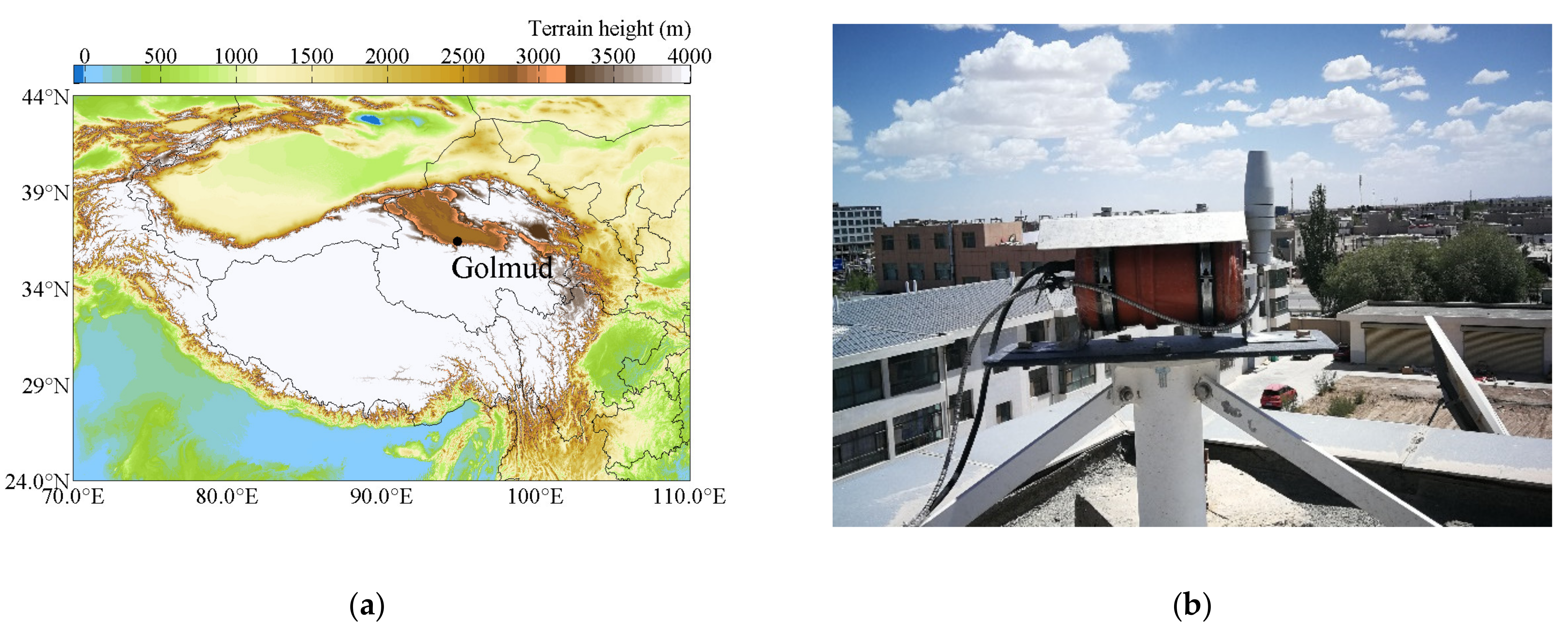
2.1. Site and Instrument

The zenith scattered light measurements were conducted from 27 May to 30 November 2020 at the Golmud meteorological station (94°54′ E, 36°25′ N; 2807.6 m above sea level), a site in the northern Tibetan Plateau (Figure 1a). This station is located at the north suburb of Golmud central city in the west of the Qinghai Province, China. It is on the southern margin of the Qaidam basin, where the natural landscape is an arid desert with a sparse vegetation cover. The Hoh Xil nature reserve is about 120 km away to Golmud’s south, and the Qarhan salt lake is about 70 km north of Golmud. The site is dominated by a continental plateau climate, characterized by low humidity, rather frequent winds and long sunny periods [46,47]. Measurements of the basic surface meteorological parameters as well as meteorological balloon soundings twice a day are performed on an operational basis. The annual averages of temperature, relative humidity and wind speed are about 5.8 °C, 32%, and 2.4 m·s−1, respectively. The prevailing wind direction is westerly.
As part of a comprehensive observation experiment on the exchange of atmospheric constituents between the stratosphere and troposphere, the Tube MAX-DOAS system (Figure 1b), set up on the roof of a four-storied building, was used to record spectra of scattered sunlight at 12 elevation angles (1°, 2°, 3°, 4°, 5°, 6°, 8°, 10°, 15°, 30°, 45°, and 90°). The instrument, developed by the Max Planck Institute for Chemistry (MPIC), Mainz, Germany, was automatically run and the zenith spectra during the twilight period were used for this study. The integration time of one individual spectrum was ~1 min. The spectrograph covered the wavelength range of roughly 300–466 nm with a spectral resolution of ~0.6 nm, operating at a detector temperature of 15 °C with fluctuations of less than 0.1 °C. The spectra of dark current and electronic offset were also collected at night for correcting each measured spectrum. A laptop was used to control the measurements. A more detailed description about the MPIC Tube MAX-DOAS instrument can be found in previous studies [48,49,50].

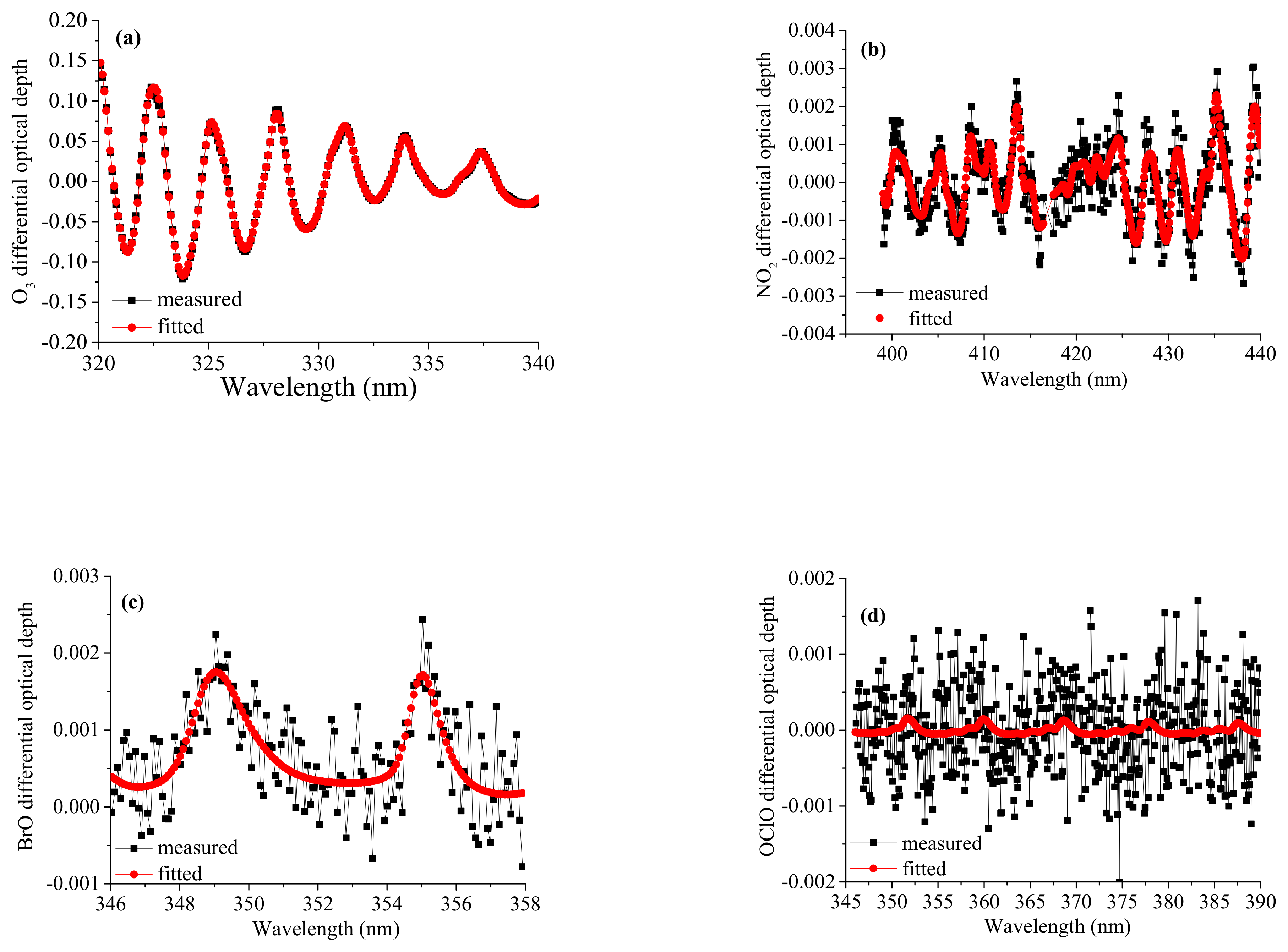
2.2. Spectral Retrieval

The differential slant column densities (dSCDs) of atmospheric trace gases can be retrieved from the measured scattered solar spectra in the zenith direction using the DOAS method [31]. The derived dSCDs of ozone (O3), nitrogen dioxide (NO2), bromine monoxide (BrO), and chlorine dioxide (OClO) represent the differences in their column densities (i.e., integrated concentrations along the light path) between the measurement spectrum and the Fraunhofer reference spectrum. In this study, a fixed zenith spectrum (at 27.6° solar zenith angle (SZA)) at 13:35 Beijing time (BJ, UTC + 8 h) on August 30, 2020 was used as Fraunhofer reference spectrum. On the basis of a non-linear least squares fitting method, the spectral analysis of the measured spectra was implemented by the QDOAS software, developed by the Royal Belgian Institute for Space Aeronomy (BIRA-IASB) [51]. The fitting parameters for the spectral analyses of O3, NO2, BrO, and OClO dSCDs are listed in Table A1, Table A2, Table A3 and Table A4. It should be noted that each measured spectrum was corrected for dark current and electronic offset and the Fraunhofer reference spectrum was spectrally calibrated by using a highly resolved solar spectrum [52]. Figure 2 shows examples of the spectral retrievals for O3, NO2, BrO, and OClO, derived from a measured spectrum at the elevation angle of 90° at 7:27 BJ on 21 July 2020. Although for most measurements the absorption structures of these trace gases can be well extracted from measured spectra, we still rejected the retrieved dSCDs once the root mean square (RMS) of spectral fitting residual was larger than a prescribed threshold. In the post processing of the dSCD data, the RMS thresholds were estimated by the balance between the quality of spectral fitting and the remaining data amount. When the RMS thresholds for O3, NO2, BrO, and OClO were set as 4 × 10⁻³, 9 × 10⁻⁴, 9 × 10⁻⁴, and 9 × 10⁻⁴, the percentages of remaining data were 72%, 69%, 72%, and 66%, respectively, on the condition of SZA ≥ 75°.

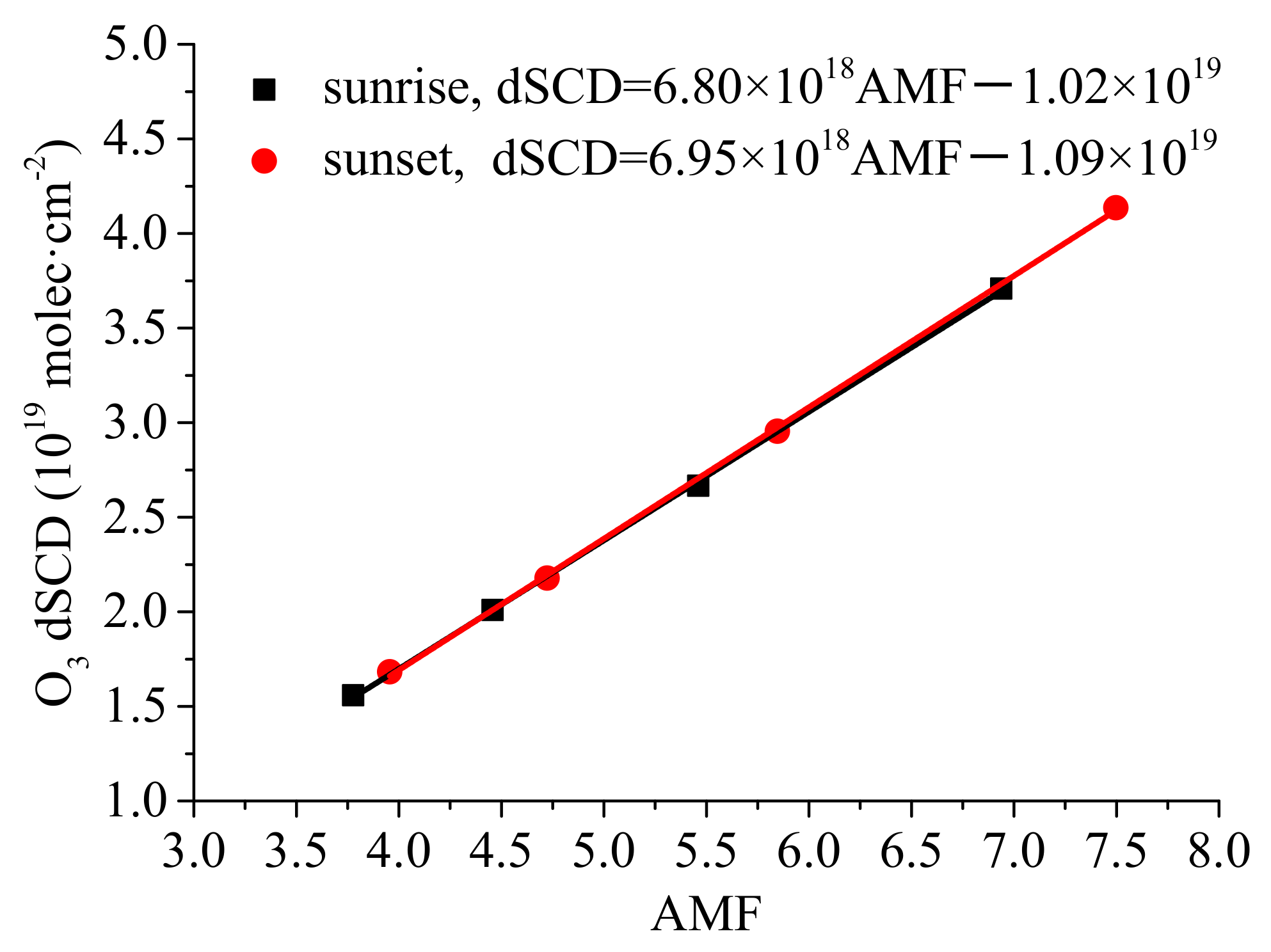
2.3. Langley Plot Method

The dSCD, derived from the spectral analysis, can be expressed by the following equation.
dSCD = SCDmeas − SCDref
where SCDmeas indicates the slant column density (SCD) of the measured spectrum and SCDref is the SCD of the Fraunhofer reference spectrum. The SCD represents the integrated concentration of the target species along the effective atmospheric light path, which depends on the solar zenith angle (SZA) for scattered sunlight measurements of stratospheric trace gases. Therefore, the SCD is usually converted to the vertical column density (VCD) through an air mass factor (AMF).
AMF = SCD/VCD
Then the dSCD can be written as:
dSCD = VCD × AMFsim − SCDref
This equation describes the so-called Langley plot method [44], which applies a linear fit between the retrieved dSCDs and the simulated AMFs (AMFsim) for sunrise and sunset on each day. In consequence, the unknown VCD and SCDref are determined by the slope and intercept of the fitted regression line, respectively. It should be noted that this method is suitable to species, such as O3, whose concentrations change very slowly with time. However, because of the rapid change in the photolysis of NO2, BrO, and OClO during the twilight, the conditions for the Langley plot method are not fulfilled for these trace gases. Therefore, the Langley plot method is not directly applied to convert the SCDs of NO2, BrO, and OClO into VCDs in this study.
In this article, the O3 AMFs are calculated by a full 3-D spherical Monte Carlo atmospheric radiative transfer inversion model (McArtim) [53]. McArtim, developed at the University of Heidelberg and MPIC, simulates individual photon trajectories based on the backward Monte Carlo method [53,54]. The various events of photon interactions at various altitudes are defined by probability distributions. McArtim can thus provide a very exact representation of the true atmospheric radiative transfer [48]. In practice, several input parameters, such as the height profiles of the target species, meteorological quantities, aerosol extinction and aerosol optical properties, are needed as input for the AMF simulations. Based on previous studies at the same or nearby stations, the single scattering albedo and asymmetry factor of aerosols as well as the surface albedo are set as 0.93, 0.60, and 0.20, respectively [46,55]. The chosen values don’t significantly change the retrieval products compared to other parameters. Therefore, we focus on the sensitivities with respect to the a-priori profiles. More details about the input parameters for the AMF simulations will be investigated in the sensitivity studies in Section 3.2.1. Figure 3 shows an example of the Langley plot method using O3 dSCDs measured on 30 August 2020. According to the linear equation in Figure 3, the O3 VCDs is 6.80 × 10¹⁸ molec·cm−2 (6.95 × 10¹⁸ molec·cm−2) for sunrise (sunset) on 30 August 2020.

2.4. OMI Product

The Ozone Monitoring Instrument (OMI) aboard NASA’s Aura satellite, launched in July 2004, orbits the earth in a polar Sun-synchronous pattern with a local afternoon equator crossing time of 13:45 [56]. It achieves complete global coverage in one day, measuring spectra in a wavelength range of 264–504 nm with a spectral resolution between 0.42 nm and 0.63 nm in a nadir-viewing mode. OMI enables the analysis of the O3 column density in the spectral range from 331.1 nm to 336.1 nm. The OMI level-3 global gridded total O3 column data (OMDOAO3e v003) are provided on a daily basis at a latitude–longitude grid of 0.25° × 0.25°. The OMDOAO3e product has been used to study long-term trends in the O3 total columns during 2004–2015 over the TP [57]. In this study, we compare the O3 VCDs retrieved from ground-based scattered solar spectra in the zenith direction with the OMI OMDOAO3e product obtained from the NASA Goddard Earth Sciences Data and Information Services Center (GES-DISC). More information on this product is available at http://disc.sci.gsfc.nasa.gov/Aura/OMI/omdoao3_v003.shtml (accessed date: 26 January 2021).

3. Results

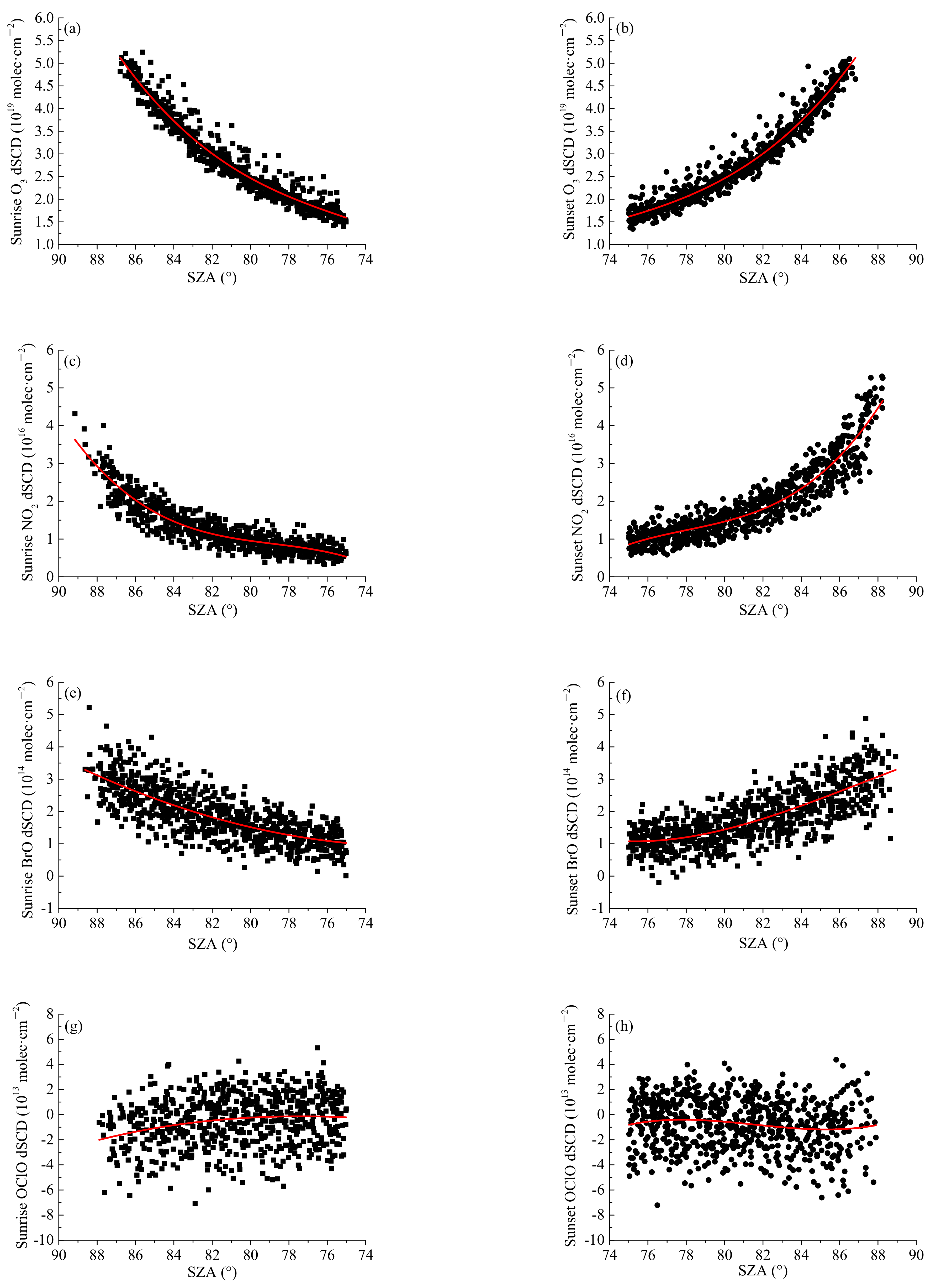
3.1. Overview on the Variations of the dSCDs with SZA

According to the prescribed thresholds, the filtered dSCDs of O3, NO2, BrO, and OClO at sunrise and sunset are shown as a function of SZA during the effective observation period (27 May–30 November 2020) in Figure 4. The nonlinear dependence of the dSCDs on the SZAs was fitted by third-order polynomials. The variations of dSCDs with SZA are nearly symmetrical between sunrise and sunset for each species (but with different absolute values for NO2). For O3, the dSCDs increase with increasing SZA, reaching ~5 × 10¹⁹ molec·cm−2 at ~87° SZA, because of the longer optical path at larger SZA. The differences of the O3 dSCDs between sunrise and sunset are small for all SZAs, typically about 1 × 10¹⁶ molec·cm−2 at 82° SZA. The medians of the O3 fit error (see [31]) during the effective observation period are 9.72 × 10¹⁶ molec·cm−2 and 9.63 × 10¹⁶ molec·cm−2 at sunrise and sunset, respectively (Figure A1). For NO2, the dSCDs also increase with increasing SZAs, up to about 2.9 × 10¹⁶ molec·cm−2 (4.5 × 10¹⁶ molec·cm−2) at 88° SZA during the sunrise (sunset). The NO2 dSCDs at sunset are systematically larger than the sunrise values as expected. The difference of the NO2 dSCDs between sunrise and sunset also increases with increasing SZA, ranging from about 3.3 × 10¹⁵ molec·cm−2 to 1.5 × 10¹⁶ molec·cm−2 between 75° and 88° SZA. The medians of the NO2 fit error during the effective observation period are 3.41 × 10¹⁴ molec·cm−2 and 3.35 × 10¹⁴ molec·cm−2 at sunrise and sunset, respectively (Figure A1). For BrO, both the sunrise and sunset dSCDs increase with increasing SZAs for the SZA range of 75°–89°, and the dependencies between 80° and 90° SZA are nearly linear. There are no obvious differences in the level of BrO dSCDs between sunrise and sunset, whose averages are 1.86 × 10¹⁴ molec·cm−2 and 1.81 × 10¹⁴ molec·cm−2 for sunrise and sunset, respectively. The medians of the BrO fit error during the effective observation period are 4.35 × 10¹³ molec·cm−2 and 4.27 × 10¹³ molec·cm−2 at sunrise and sunset, respectively (Figure A1). The time series of the fit absolute errors and relative errors of O3, NO2, BrO, and OClO dSCDs at sunrise and sunset are also shown in Figure A1. For OClO, the sunrise and sunset dSCDs almost show a constant level of ~−1 × 10¹³ molec·cm−2, which is smaller than the typical OClO fit errors of about 1.4 × 10¹³ molec·cm−2. We estimate the OClO detection limit to be twice the fit error, i.e., 2.8 × 10¹³ molec·cm−2. The OClO, as a kind of O3 depleting substances, is important in the stratospheric atmospheric chemistry. In spite of the low values, we show the OClO results in this study for two reasons: (1) The parameters and the procedure of the OClO spectral retrieval can provide a reference for OClO DOAS spectral retrieval over the TP in future, especially also during winter. Under such conditions, the polar vortex might occasionally reach to the measurement location. The possibly seasonal enhancements of OClO dSCDs might be observed at larger SZA over the TP in future. (2) Although we can’t obtain significant temporal variations of OClO dSCDs due to the OClO abundance lower than the detection limit of the instrument, the result (or conclusion) is important, because it shows that the DOAS spectral analysis works well and the expected result (i.e., very low OClO abundance in summer and autumn over the TP) is obtained.

3.2. O3 Vertical Column Densities (VCDs)

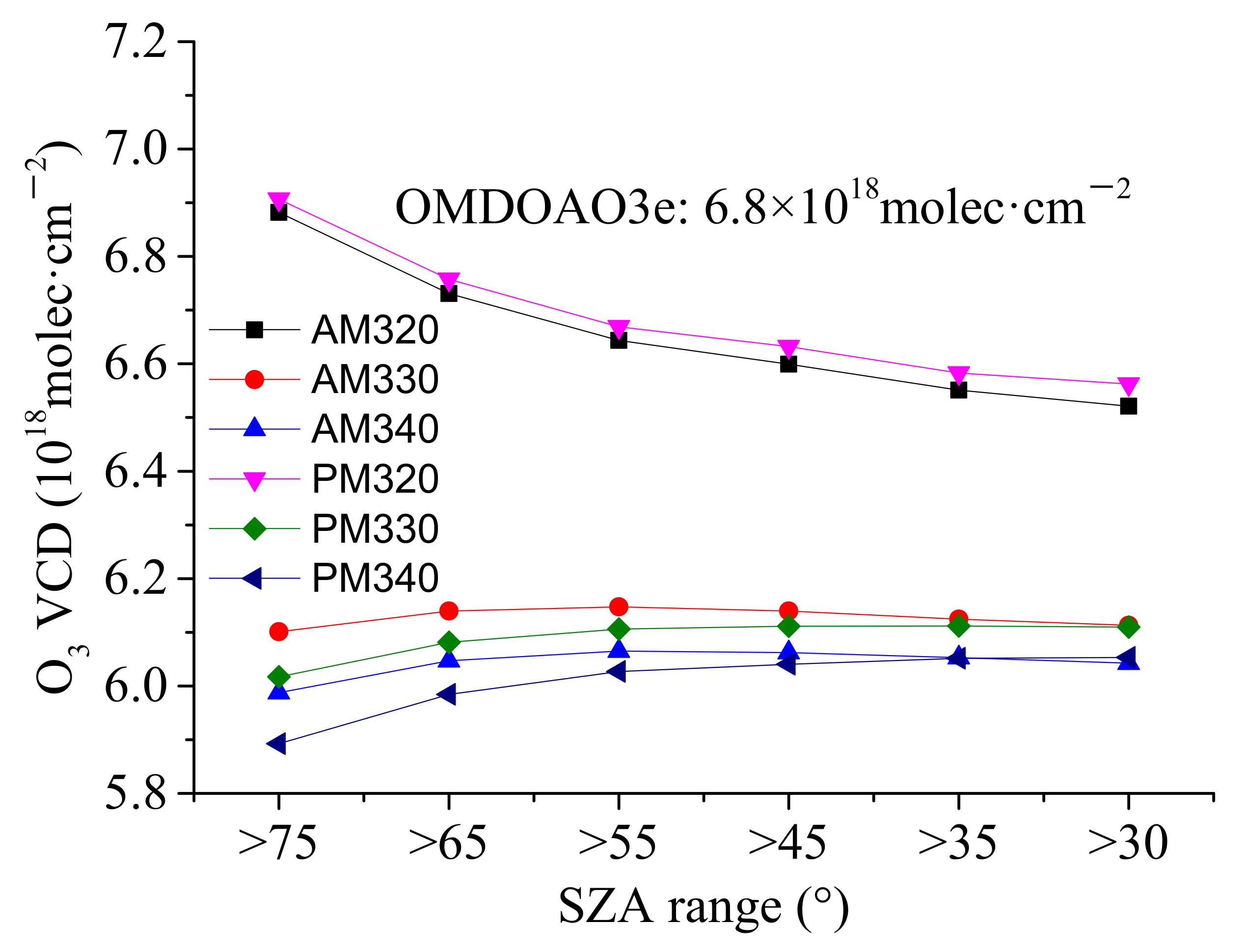
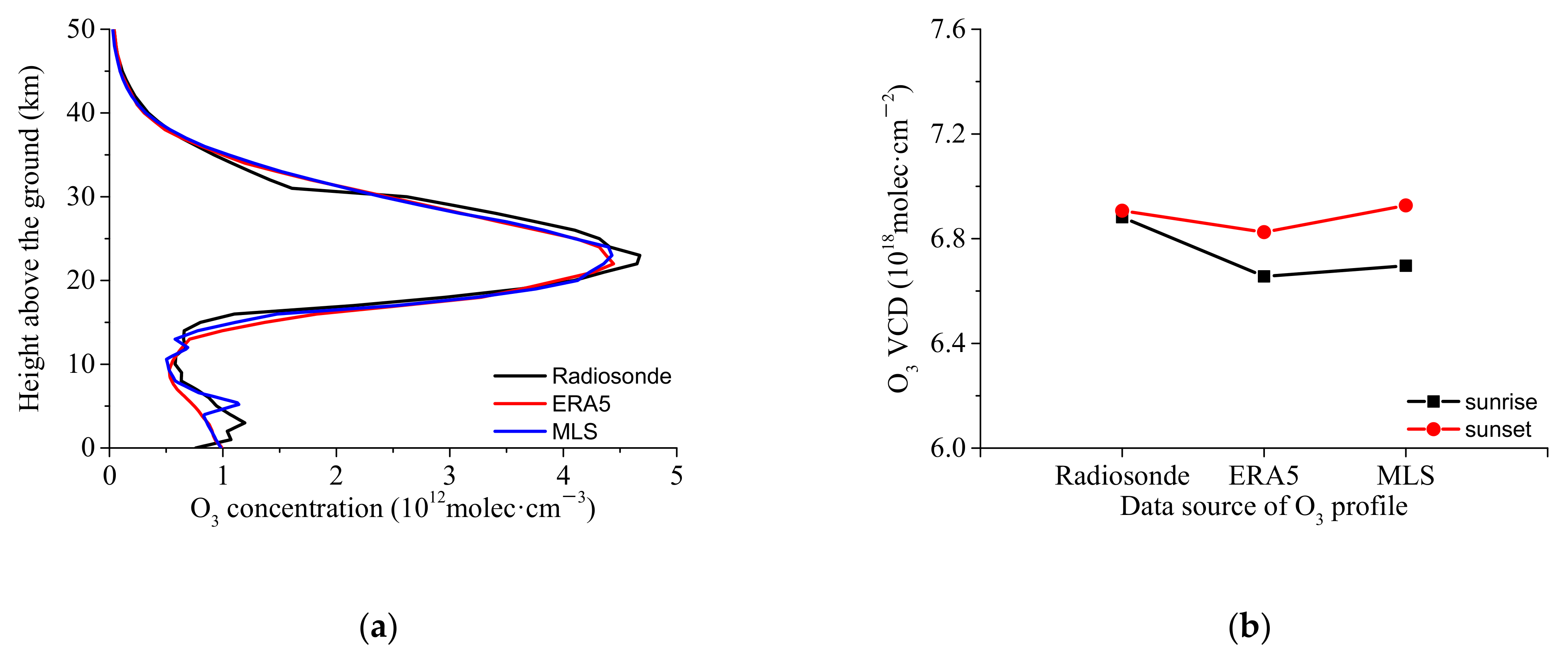
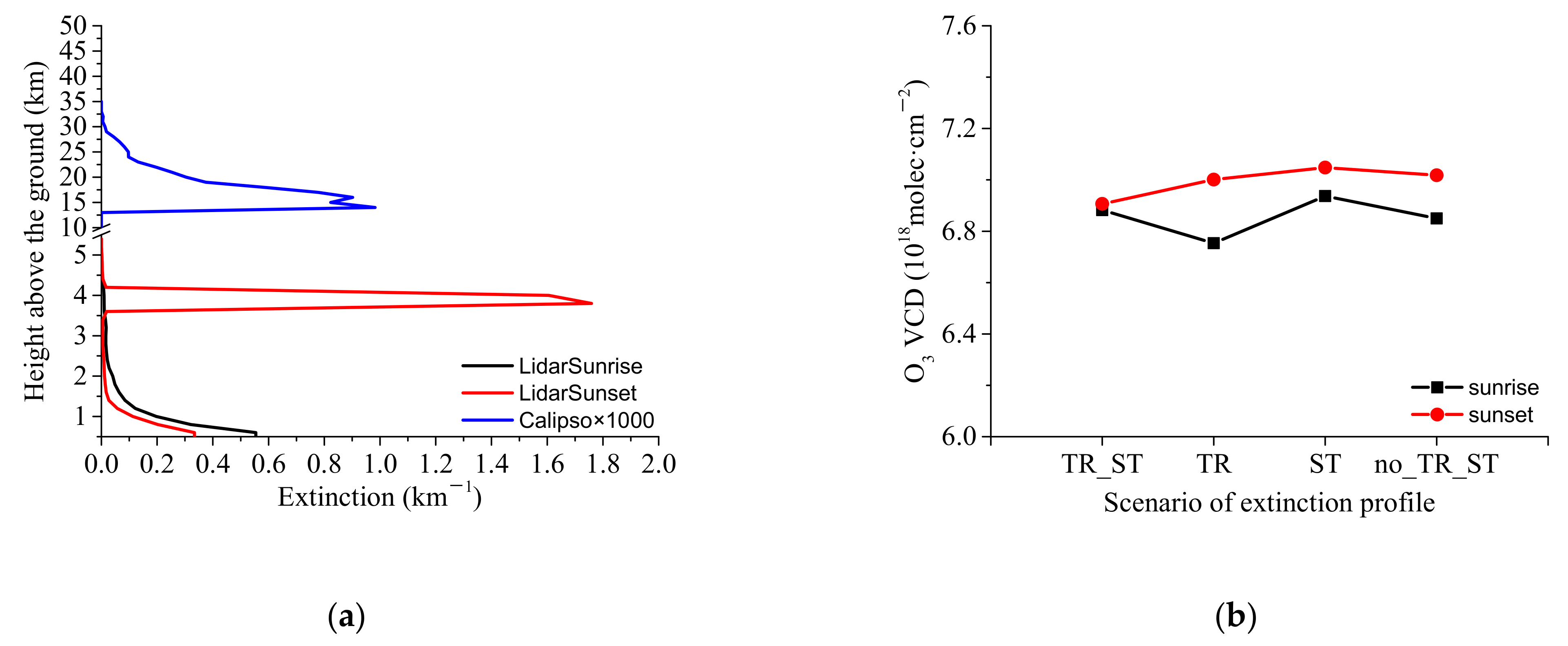
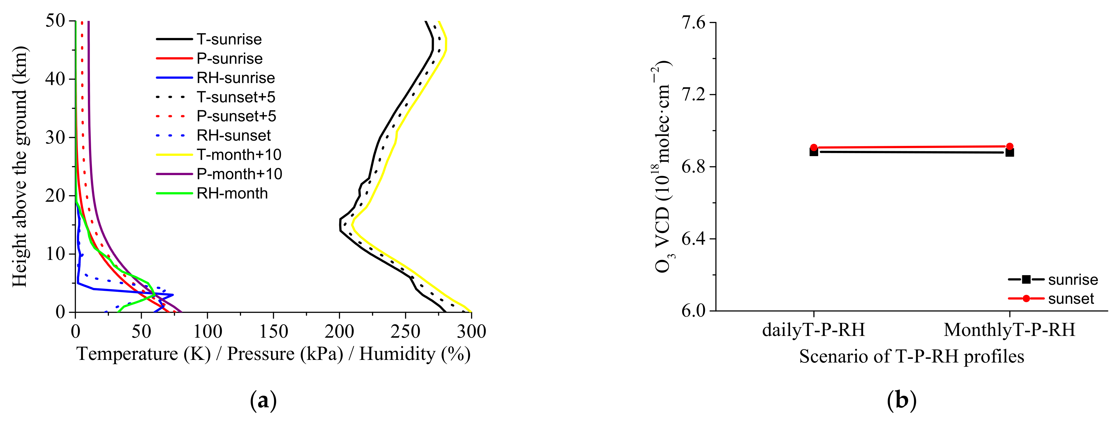
3.2.1. O3 VCD Sensitivities to AMF Simulation Parameters

By applying the Langley plot method, the O3 VCDs during sunrise and sunset are derived. However, the resulting O3 VCDs depend on the calculated AMFs, which themselves depend on several input parameters, such as simulation wavelength, SZA range, and a priori vertical profiles of O3, aerosol extinction, temperature, pressure, and relative humidity (Table 1). It should be noted that the influences of the single scattering albedo and asymmetry factor of the aerosols as well as the surface albedo are not the focus of this study because they don’t significantly influence the retrieval results in summer and autumn at Golmud. We investigated the sensitivities of the O3 VCDs to these parameters on 30 August 2020, which is the same day used for selecting the fixed Fraunhofer reference spectrum. Figure 5 shows the sensitivity of the derived O3 VCDs on the SZA range and the wavelength at which the AMFs were simulated (case 1 in Table 1). The O3 VCD gradually tends to level off from a SZA range of >75° to >30°. For a given SZA range, the O3 VCDs are larger for smaller wavelengths in the range of 320–340 nm. For the selection of the SZA range and simulation wavelength, we follow two primary principles: (a) we want to give largest weight to high SZAs, because for these SZAs the measurement sensitivity is highest. Therefore, we chose the SZA range of >75°; (b) for the simulation wavelength we chose the 320 nm, because the spectral fit is most sensitive to small wavelengths with the strongest ozone absorptions. For this wavelength choice, the best agreement with the O3 VCD from satellite observation (OMDOAO3e) is also found.
The influences of the O3 profiles from different data sources on the derived O3 VCDs are shown in Figure 6 (case 2 in Table 1). The heights of the O3 concentration peaks are very similar for measurements from radiosonde, ECMWF Reanalysis version 5 (ERA5), and the Microwave Limb Sounder (MLS) satellite, but the peak concentration from the radiosonde is ~5% higher than for the other two datasets. The O3 profile of ERA5 below 15 km is smoother than those from the radiosonde and MLS measurements. The sunrise O3 VCDs range from 6.66 × 10¹⁸ molec·cm−2 (ERA5) to 6.88 × 10¹⁸ molec·cm−2 (radiosonde), and the sunset O3 VCDs range from 6.83 × 10¹⁸ molec·cm−2 (ERA5) to 6.93 × 10¹⁸ molec·cm−2 (MLS). The relative deviations of the O3 VCDs between ERA5 and OMDOAO3e are about 2.1% and 0.4% for sunrise and sunset on 30 August 2020, respectively. Owing to the high temporal resolution and open access of the ERA5 dataset, we prefer to use monthly ERA5 O3 profiles in our study.
Figure 7 shows the vertical aerosol extinction profiles as well as the O3 VCDs derived from the Langley plot method for the different aerosol scenarios (case 3 in Table 1). On the whole, the aerosol extinction in the troposphere measured by the Lidar decreases with height for both sunrise and sunset, but there was a cloud layer around 3.80 km at sunset on 30 August 2020. The climatic extinction profile in the stratosphere over the TP can be extracted from the Cloud-Aerosol Lidar and Infrared Pathfinder Satellite Observation (Calipso) [58]. Therefore, the extinction profile observed by the Calipso satellite instrument in July 2020 is taken as the stratospheric extinction profile in this study. Through comparing the O3 VCDs for the aerosol scenarios of TR and no_TR_ST, we find that the O3 VCDs are lower in the former scenario, i.e., containing the tropospheric extinction profile. However, when comparing the O3 VCDs for the aerosol scenarios of ST and no_TR_ST, the O3 VCDs are higher in the former scenario, i.e., including the stratospheric extinction profile. Although there are orders of magnitude difference in the absolute values of the aerosol extinction between the troposphere and stratosphere, the sensitivities of the O3 VCDs to tropospheric and stratospheric aerosol profiles are almost equivalent (but of opposite sign). This is probably related to the influences of two factors, i.e., the longer light path in the stratosphere for zenith DOAS measurement during twilight periods and the higher abundance of aerosol in the troposphere. These two aspects have an almost similar influence on the O3 VCDs for our measurements. However, this might be different for other measurement stations. According to the O3 VCDs for the aerosol scenario of TR at sunrise and sunset, it is also found that there are no significant deviations caused by the appearance of the cloud. Thus, finally, we select the aerosol extinction profile scenario of TR_ST including both tropospheric and stratospheric aerosol profiles for the O3 AMF simulations.
The sensitivities of O3 VCDs to the profiles of temperature (T), pressure (P), and relative humidity (RH) used for the O3 AMF simulation are presented in Figure 8 (case 4 in Table 1). The differences in the daily and monthly profiles of temperature and pressure are small, but there are significant differences between daily and monthly values of the relative humidity below 15 km. However, the O3 VCD remains almost unchanged, even if we use the monthly averaged profiles of temperature, pressure, relative humidity from the operational meteorological soundings. Therefore, it is reasonable to select the observed monthly T-P-RH profile for the O3 AMF simulations.

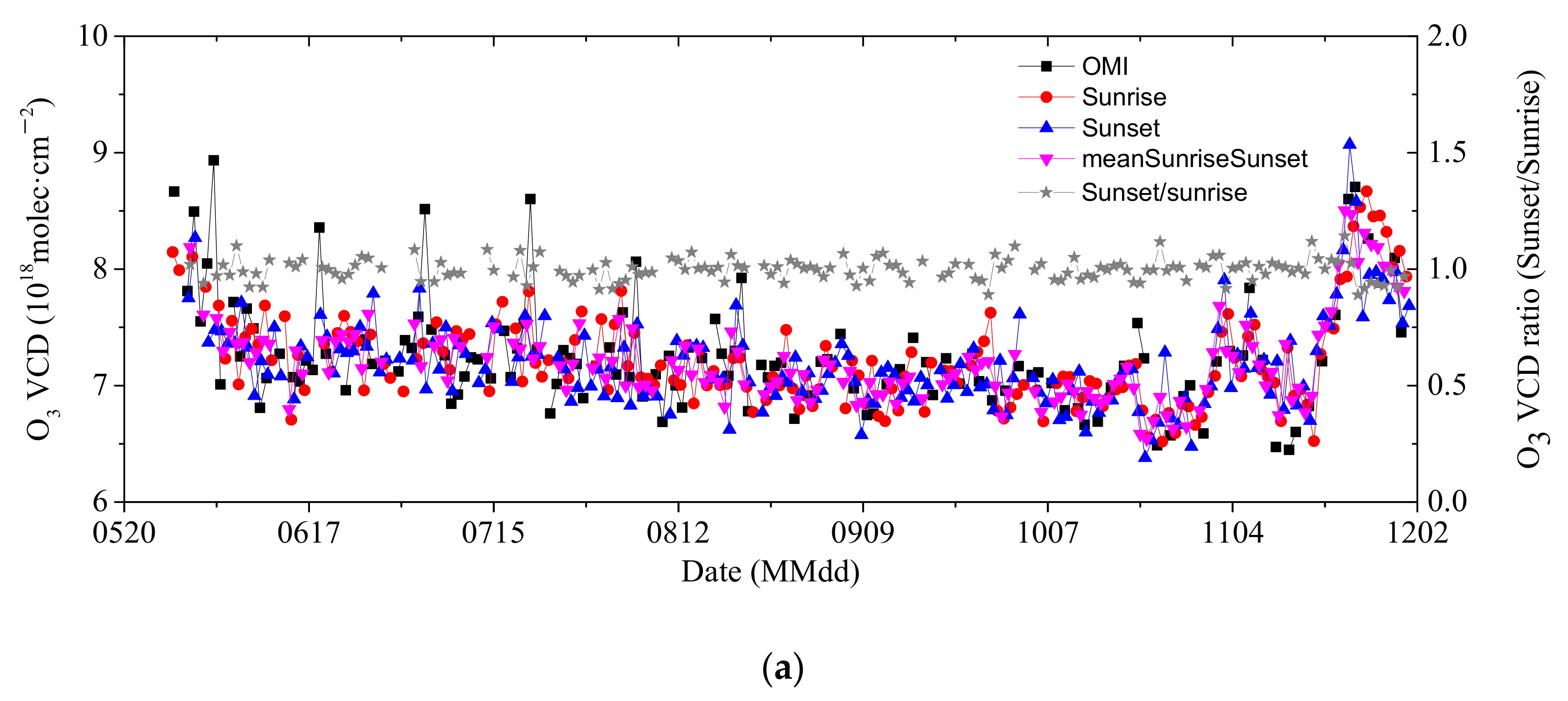
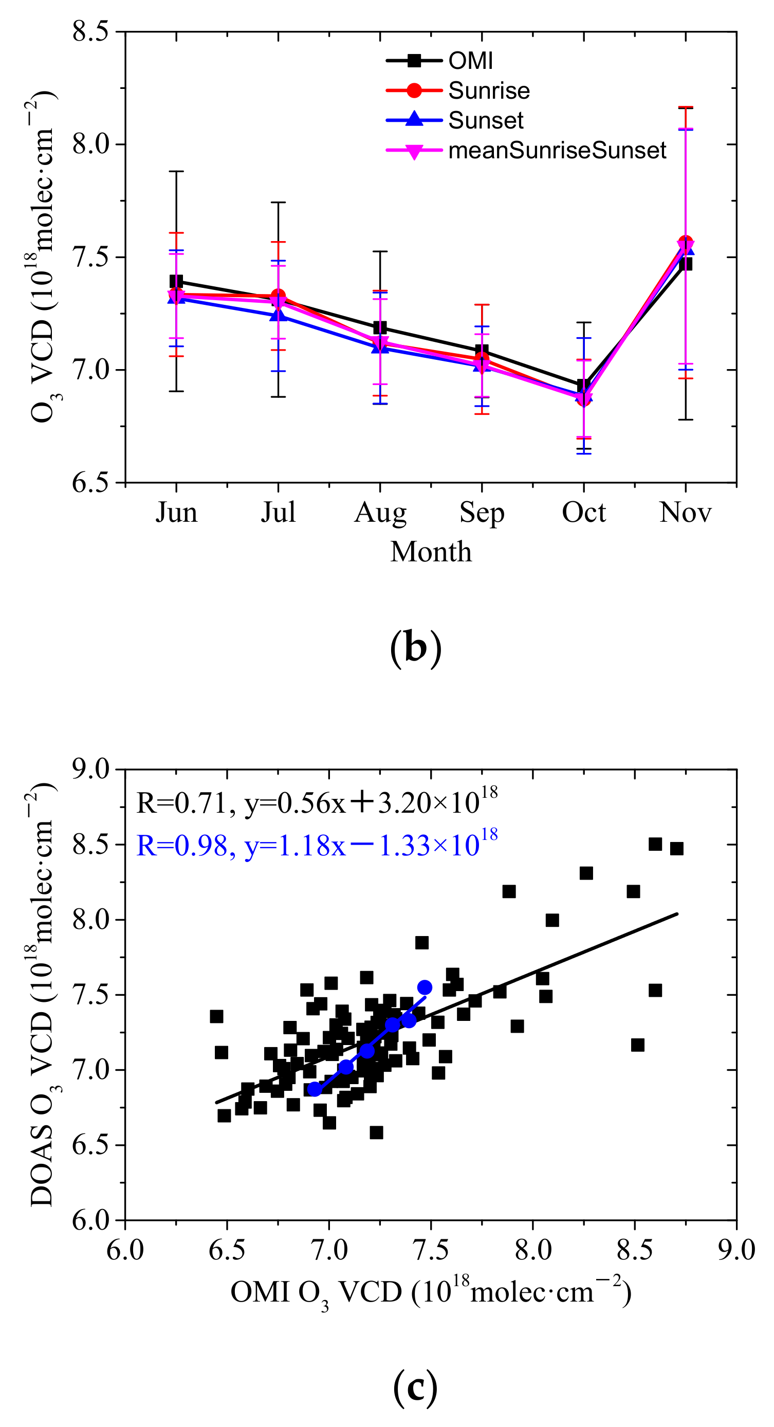
3.2.2. Variation of the O3 VCD and Comparison with the OMI Product

Based on the Langley plot method with the optimal parameters for the O3 AMF simulations (case 5 in Table 1), we obtained the O3 VCDs at sunrise and sunset of each day in summer and autumn 2020 (Figure 9a). The ratios of the O3 VCDs at sunset to those at sunrise are nearly equal to 1 for each day, indicating that the differences of stratospheric O3 between sunrise and sunset are very small. Their daily averages from ground-based zenith DOAS measurement are consistent with the O3 VCDs from the OMI OMDOAO3e product extracted within the grid cell covering the Golmud site. The regression analysis between the two datasets yields a correlation coefficient R = 0.71 (Figure 9c). The correlation coefficient is substantially smaller than unity, probably because the variability of the O3 VCDs during the observed period is rather small. The agreement can be further confirmed by the comparison of the monthly O3 VCDs with a correlation coefficient R = 0.98 (Figure 9b,c). The differences in correlation coefficient for daily and monthly O3 VCDs between the two datasets have at least two reasons: (1) There are suddenly high values for the OMI daily O3 VCDs; (2) The day-to-day variability has a smaller effect on the correlation of the monthly mean O3 VCDs. The monthly O3 VCDs in May 2020 are not shown because of very limited data during this month. The mean O3 VCDs from June to November 2020 are 7.21 × 10¹⁸ molec·cm−2 and 7.18 × 10¹⁸ molec·cm−2 at sunrise and sunset, respectively. The standard deviations of the monthly O3 VCDs between sunrise and sunset are close to each other. In addition, there are similar trends for the monthly O3 VCDs between the ground-based and satellite observations, ranging from a minimum of 6.9 × 10¹⁸ molec·cm−2 in October to 7.5 × 10¹⁸ molec·cm−2 in November. This seasonal variation is consistent with previous studies investigating the multi-year-average of the O3 VCDs over the TP, caused by complex dynamical and chemical factors [15,59]. The differences of the monthly O3 VCDs derived by the two methods are within 1%, but the standard deviations of the O3 VCDs from OMI are systematically larger than the results from the ground-based zenith DOAS. The consistency of the two datasets is similar or better than typical comparisons of the total ozone between ground-based remote sensing measurements (Dobson, Brewer, SAOZ) and satellite products at Arosa [60]. In summary, the O3 VCDs retrieved from ground-based zenith DOAS measurements agree well with the OMI satellite product, clearly presenting the monthly variation of O3 VCDs around the period of the O3 summer low in the northern TP.

3.3. NO2 Vertical Column Densities (VCDs)

Because of the rapid photolysis of NO2 and its reservoir species during twilight as well as the fact that the measurements were limited to SZA < 90°, a modified method was used to calculate the NO2 VCDs at SZA = 90° using the following formula.
VCDSZA = 90° = (dSCDSZA = 90° + SCDref)/AMFSZA = 90°
where dSCDSZA = 90°, i.e., the NO2 dSCD for a SZA of 90°, is derived by the extrapolation through a third-order polynomial fit of the dSCDs as function of the SZA at each sunrise and sunset between SZA of 75° and 90°. First, the SCDref is determined by the Langley plot method for each day, simultaneously taking into account the measured NO2 dSCDs at sunrise and sunset in the SZA range of 60–80°. This SZA range was chosen due to the weaker photochemical effects for these SZAs. Only results of NO2 SCDref were kept when the square of correlation coefficient R between the dSCDs and AMFs (R2) was larger than 0.8. The remaining data were further skipped when the slope of the Langley plot was out of range of the slope’s mean ± standard deviation. Finally, 33% of the total days met the screening principle during the effective observation period. From the remaining results, we calculated the average of the NO2 SCDref during our observation period as 3.70 × 10¹⁵ molec·cm−2. This value was then used in equation (4). The NO2 AMFs for each sunrise and sunset period were extracted from the look-up table (LUT) of the Network for the Detection of Atmospheric Composition Change (NDACC) [61]. Therein, besides the default parameters, the wavelength for the simulation of the atmospheric radiative transfer and the surface albedo were set as 428 nm and 0.20, respectively.
According to the aforementioned method, we obtained the NO2 VCDs at 90° SZA from 27 May to 30 November 2020 (Figure 10a). As expected, the NO2 VCDs at sunset are systematically higher than those at sunrise, with an average ratio of ~1.56, which is related to the photolysis of N2O5 [6]. We also show the total NO2 VCDs from the OMI-L3 cloud-screened product (OMNO2d V3, screened for cloud fractions below 30%) at the grid cell of the Golmud site by the black squares in Figure 10a. More details about the OMNO2d product can be found in our previous study [62]. There are some low outliers in the OMI product in summer from a statistical perspective. It is not clear that the outliers of the OMI product are caused by the influence of clouds, the complex terrain over the TP, or other factors. The overall temporal trends of the NO2 VCDs obtained from the ground-based zenith DOAS and the OMI satellite observations are in agreement. They gradually decrease with time during the effective observation period. Figure 10b shows the correlations of the daily NO2 VCDs between the two datasets. The correlation coefficient RSunset (=0.53) between the ground-based measurements at sunset and the OMI satellite observations is larger than that at sunrise (RSunrise = 0.24). The deviations between the two data sets are probably related to the differences in the spatial and temporal representativeness of the NO2 VCDs separately obtained by the two methods, and the accuracy of the zenith DOAS and OMI satellite retrieval products over the TP. Furthermore, we calculated the monthly means and standard deviations of the NO2 VCDs from June to November (Figure 10c). According to the larger standard deviations (uncertainties) of the OMI satellite products, the precision of the OMI satellite products is lower than the ground-based zenith DOAS observation. However, a similar overall monthly variation is found in both datasets (Figure 10c). With respect to the monthly NO2 VCDs averaged between sunrise and sunset, the maximum (3.40 × 10¹⁵ molec·cm−2) is found in July. The strong monthly variation of the NO2 VCDs is consistent with results from multi-year (1997–2016) monthly averaged stratospheric NO2 VCDs at Kiruna, Sweden, but the maximum is smaller than those observed in Kiruna [63]. For the daily NO2 VCDs, the correlation is smaller than for the monthly NO2 VCDs (RSunrise = 0.86 and RSunset = 0.97, see Figure 10d). The monthly NO2 VCDs observed by OMI are systematically larger (smaller) than those at sunrise (sunset) measured by ground-based zenith DOAS from June to September. For the measurements over the TP, the NO2 VCDs during the satellite overpass are better represented by the sunset observations.

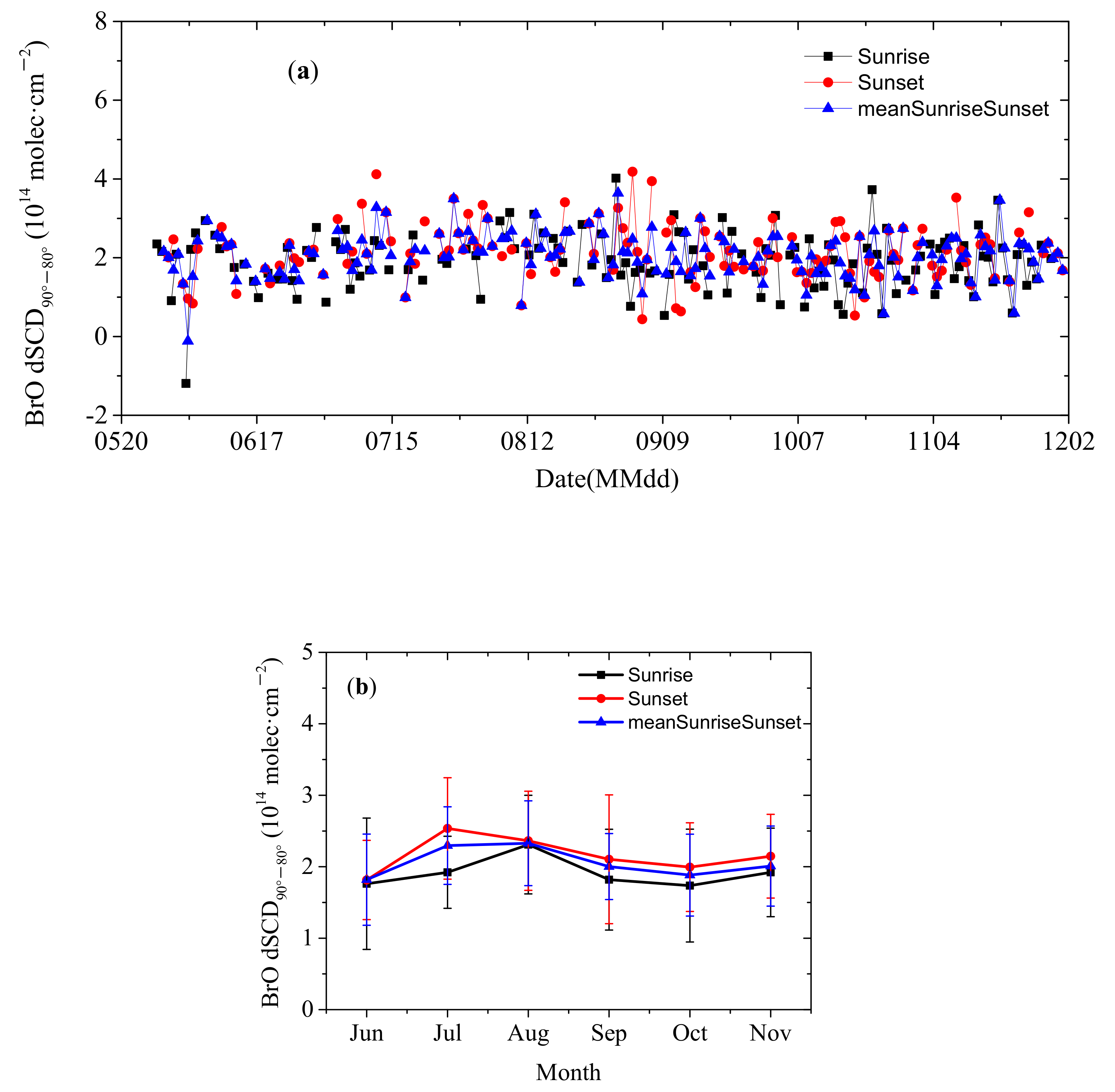
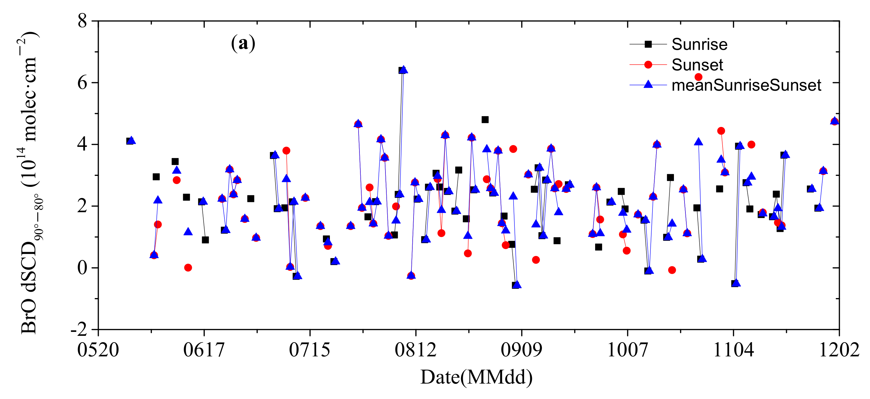
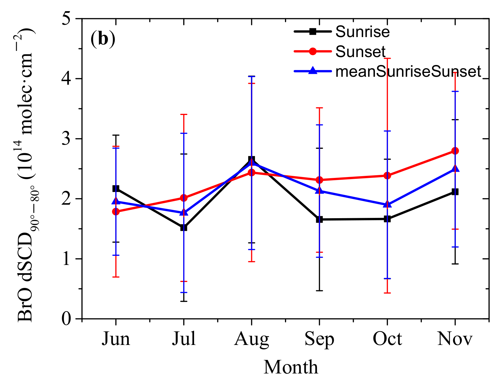
3.4. Temporal Variation of the BrO dSCDs

To analyze the temporal variation of stratospheric BrO, we calculated the difference in the BrO slant column densities between 90° and 80° SZA, abbreviated as dSCD90°–80°. This choice was made primarily in order to optimize the signal-to-noise ratio of the differential BrO absorption and maximize the sensitivity of the observation to the stratospheric part of the BrO profile [12]. The calculation procedure of BrO dSCD90°–80° is as following:
dSCD90°–80° = SCD90°–SCD80°
=(dSCD90° + SCDref)–(dSCD80° + SCDref)
=dSCD90°–dSCD80°
Firstly, the filtered BrO dSCDs retrieved from the measured spectra at elevation angles of 30°, 45°, and 90° are plotted as a function of the SZA, separately for sunrise and sunset on each day. Here we also consider the elevation angles of 30° and 45° (in addition to the zenith direction) in order to increase the number of data points, because for the BrO analysis the fit error is larger than for the analyses of O3 and NO2. The consideration of these additional non-zenith directions is justified by the fact that no systematic difference of the BrO dSCDs from those for zenith direction is found indicating a negligible amount of BrO in the troposphere. Then, once the largest valid SZA is larger than 87°, a linear curve is fitted to the BrO dSCDs in the SZA range from 80° to 90°; Finally, the BrO dSCD90° and dSCD80° are obtained from the fitted linear curve.
According to the aforementioned method, the time series of the daily and monthly BrO dSCD90°–80° for sunrise and sunset as well as the mean value between sunrise and sunset are shown in Figure 11 (Figure A2 shows the same results, but only the retrieved BrO dSCDs for 90° elevation angle were used to obtain the BrO dSCD90°–80°). On the monthly scale, the standard deviations of the BrO dSCD90°–80° are also shown, which represent the overall statistical uncertainties of the BrO dSCD90°–80°. The peak values of the monthly BrO dSCD90°–80° appeared in August and July for sunrise and sunset, respectively. The monthly means of the BrO dSCD90°–80° for sunrise and sunset are in the range of 1.82~2.33 × 10¹⁴ molec·cm−2, with the average of 2.06 × 10¹⁴ molec·cm−2 during the period from June to November 2020. The biggest difference of the monthly BrO dSCD90°–80° between sunrise and sunset was found to be 6.14 × 10¹³ molec·cm−2 in July. The level of the BrO dSCD90°–80° at Golmud is found to be higher than those observed at other mid-latitude stations like Bremen (53° N) in summer and autumn of 1994–1995, but the monthly variations for the latter were found to be more significant from June to November [40]. Compared to the modeled results at a similar latitude in Huelva, Spain (37° N) in the summer and autumn of 1998–1999, the BrO dSCD90°–80° in this study are still higher, but they show a similar monthly variation [12]. According to the previous studies, the day-to-day variability in the BrO column at a given location is largely a result of changes in the total inorganic bromine (Bry) column, but the seasonal and latitudinal variations of BrO are basically due to the combined effects of variations in the Bry column due to transport and variations of the bromine partitioning due to chemistry [12].

4. Discussion

During the effective observation period, the retrieved dSCDs of O3, NO2, and BrO increased with increasing SZAs as expected due to the longer optical path at larger SZA [37,64]. The OClO abundance in summer and autumn over the TP was lower than the detection limit of the measurements, and it might be interesting to investigate the possibility of detecting enhanced OClO dSCDs at higher SZAs in the future.
We first investigated the sensitivities of the O3 VCDs to O3 AMF simulation parameters over the TP, by applying the Langley plot method. The strong wavelength dependence of the O3 VCDs is related to the nonlinearities caused by the strong ozone absorption at short wavelengths, especially for high SZAs. We found no significant deviations of the derived O3 VCDs when monthly O3 profiles were used, probably because the O3 profiles in the stratosphere are rather stable during the observation period. Additionally, the influence of different aerosol profiles on the O3 AMFs was investigated. For different tropospheric and stratospheric aerosol profiles rather small differences of the derived O3 VCDs were found. Even the appearance of tropospheric clouds has a negligible effect. The profiles of temperature, pressure, and relative humidity have only a negligible effect on the O3 AMF calculation, probably due to no significant variations in these profiles above the height of the thermodynamic tropopause. On the basis of the final selected optimal AMF simulation parameters, O3 VCDs from ground-based zenith DOAS were obtained by the Langley plot method, and good agreement with OMI satellite O3 VCD product is found indicating that the total O3 columns measured by zenith DOAS can be used for the validation of satellite products [65]. The monthly variation of O3 VCDs in summer and autumn over the TP was found to be consistent with the seasonal characteristics of the O3 VCDs in mid latitudes of the Northern hemisphere, reflecting the balance of dynamical transport and photochemical processes [66].
The NO2 VCDs at 90° SZA for sunrise and sunset were calculated by a modified Langley plot method. Similar to studies of stratospheric NO2 at Kiruna (67.8° N) in the Arctic and other locations (e.g., Reykjavik (64° N), Eureka (80° N)) [38,63,67], the NO2 VCDs at sunset were systematically larger than those at sunrise, owing to the photolysis of dinitrogen pentoxide (N2O5, a reservoir species of NO2) under sunlight conditions [6]. The monthly NO2 VCDs gradually decreased from June to November, and good agreement with the OMI satellite product is found. But the maximum and decreasing rate of the monthly NO2 VCDs were different from the results at other locations, e.g., Kiruna. These differences are probably caused by the differences of the complex dynamic and chemical processes over the TP. In order to better understand these differences more research should be carried out, e.g., through the combination of measurements and models in the future. In addition, the occurrence of several outliers in the OMI NO2 product in summer is probably caused by the influence of clouds over the TP, indicating that more ground-based observations over the TP are needed to better validate satellite products in future.
BrO dSCDs90°–80° were obtained to characterize the temporal variation of stratospheric BrO. Compared with the BrO abundance observed at other high- and mid-latitude stations before 2000, the average level of the BrO dSCD90°–80° in this study (with minor fluctuations from June to November) was found to be higher [12,40]. The monthly BrO dSCD90°–80° showed peaks in summer and slowly increased after October, similar to the simulated results at the same latitude site of Huelva, Spain [12]. The anti-correlation (i.e., negative correlation) of the monthly variations between BrO and NO2 was found not to be significant, in contrast to other stations in mid to high latitudes, and especially polar regions [40,63]. This implies that the BrO variations in summer and autumn over the TP were not dominated by reactions between NO2 and BrO through the reservoir species BrONO2. Dynamical variations and transport processes are probably important factors for the monthly variation in BrO over the TP.
In this study, the temporal variations of O3 and its depleting substances (NO2 and BrO) over the TP were analyzed. The interpretation of their relationships is complex due to the combined effects of dynamical and chemical processes [16,38]. However, the interrelations among the four species for the specific conditions of the TP should be further investigated by combining measurements with atmospheric model simulations, which could probably derive meaningful conclusions about ozone depletion as well as the stratospheric atmospheric chemistry during the “ozone valley” over the TP.

5. Conclusions

Ground-based zenith scattered light DOAS measurements were conducted in summer and autumn (27 May–30 November) 2020 at Golmud, a site in the northern Tibetan Plateau (TP). Differential slant column densities (dSCDs) of O3, NO2, BrO, and OClO were simultaneously retrieved from scattered solar spectra in the zenith direction during the twilight period by the DOAS technique. For O3 and NO2, vertical column densities (VCDs) were also derived. The O3 VCD was determined by applying the Langley plot method during each twilight period. We analyzed the sensitivities of O3 VCDs to different parameters of the O3 air mass factor (AMF) simulation and determined optimum settings for these parameters. The NO2 VCDs at 90° SZA for each sunrise and sunset were calculated by a modified Langley plot method. For BrO, time series of dSCD90°–80° for each sunrise and sunset were obtained, as in previous studies. For OClO, the derived dSCDs were close to zero and well below the detection limit. This was expected because during that season the stratospheric temperatures were above the formation temperature of polar stratospheric clouds. Nevertheless, this finding is still of importance, because it indicates the maturity of the OClO analysis to be applied to measurements in periods when enhanced OClO abundances can be expected. Based on the retrieved trace gas dSCDs and VCDs, we investigated the corresponding abundances and temporal variations. The VCDs of O3 and NO2 were also compared to OMI satellite observations. The main findings are summarized below.
  • O3 VCDs, derived by the Langley plot method, are sensitive to the wavelength, the a priori O3 profile, and the aerosol extinction profile used in the AMF simulation model as well as the SZA range covered by O3 dSCDs. In contrast, the O3 VCDs are almost insensitive to the chosen profiles of temperature, pressure, and relative humidity.
  • The derived O3 VCDs matched well with the OMI satellite product, with a correlation coefficient R = 0.98 for the monthly O3 VCDs. One possible reason, for the differences between the two data sets, was the difference in the spatial and temporal representativeness of the O3 VCDs obtained by the zenith DOAS and the OMI satellite. The differences in O3 VCDs between sunrise and sunset are very small. The mean O3 VCDs from June to November 2020 are 7.21 × 10¹⁸ molec·cm−2 and 7.18 × 10¹⁸ molec·cm−2 at sunrise and sunset, respectively. The derived O3 VCDs show a considerable monthly variation in summer and autumn over the northern TP, ranging from a minimum of 6.9 × 10¹⁸ molec·cm−2 in October to 7.5 × 10¹⁸ molec·cm−2 in November.
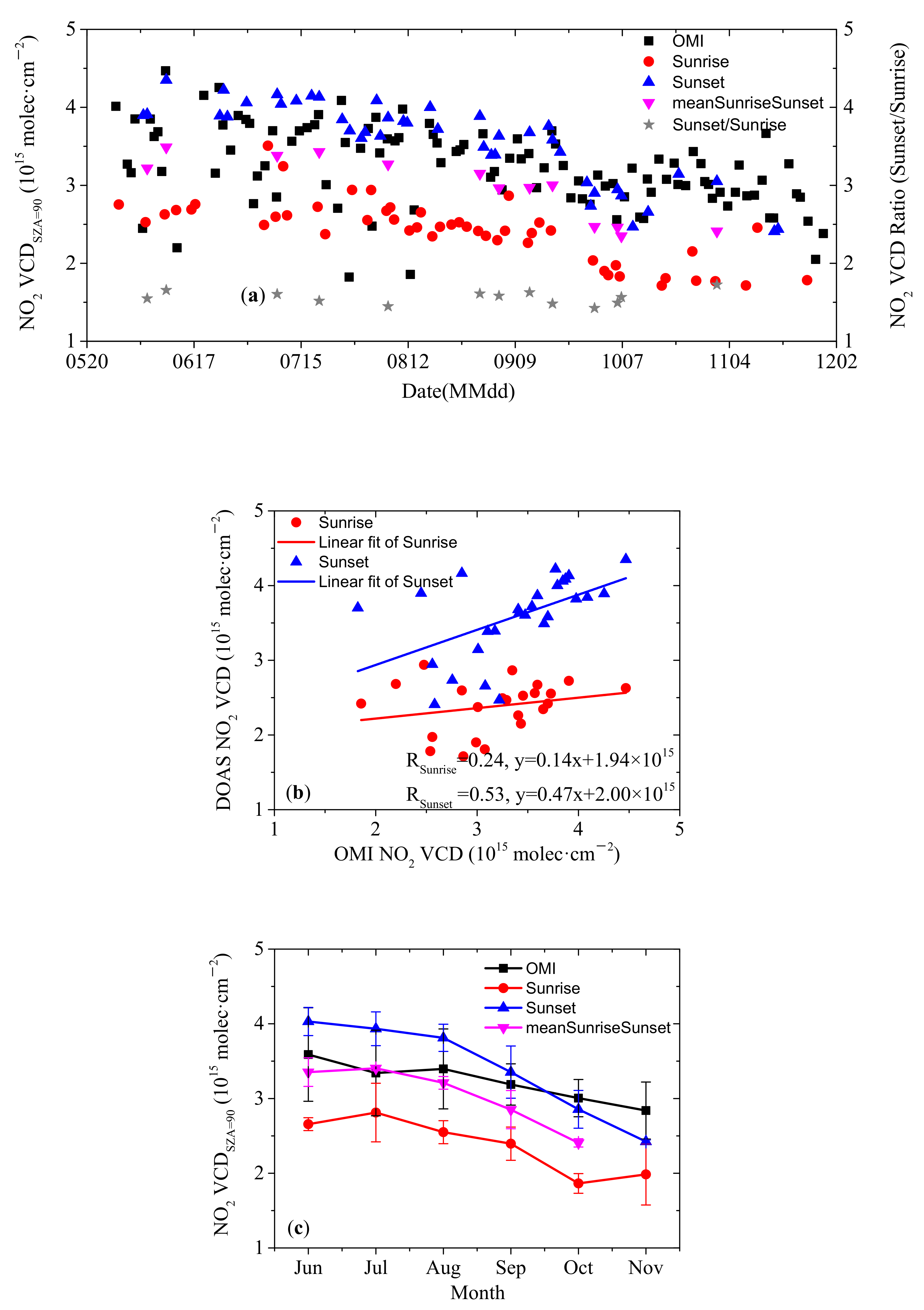
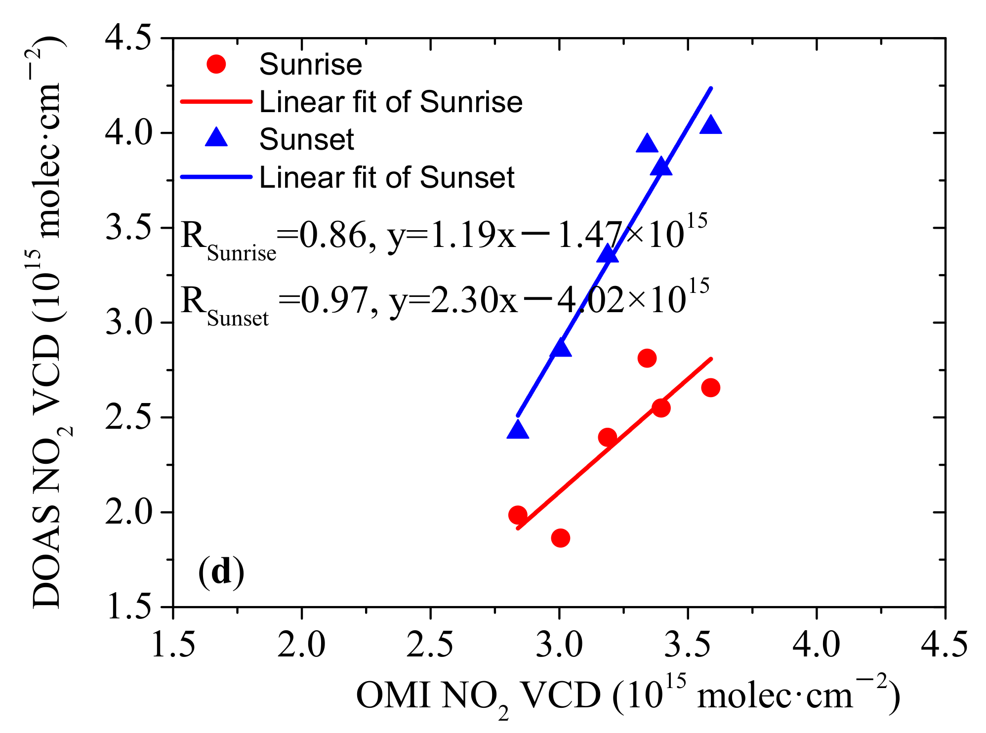
  • As expected, the NO2 VCDs for 90° SZA at sunset were systematically larger than those at sunrise with an average ratio of ~1.56, owing to the N2O5 photolysis under sunlight conditions. During the observation period the NO2 VCDs gradually decreased with time. Although the temporal trends of the NO2 VCDs obtained from the ground-based zenith DOAS and OMI satellite observations agree well, there are significant differences in the correlation coefficients of the NO2 VCDs at sunrise and at sunset between ground-based measurement and OMI satellite observation, with RSunrise = 0.86 and RSunset = 0.97 for monthly NO2 VCDs, respectively. This indicates that for the measurements in the TP, the NO2 VCDs during the satellite overpass are better represented by the sunset observations. The correlations between the two data sets are partly connected with the accuracy of NO2 VCDs retrieved from the ground-based zenith DOAS and OMI satellite observations.
  • The average level of BrO dSCD90°–80° at Golmud was 2.06 × 10¹⁴ molec·cm−2 during the period of June–November 2020 with the highest values in August and July for sunrise and sunset, respectively. Our results did not show a pronounced anti-correlation of the monthly variations between BrO and NO2, implying the importance of dynamical transport processes, rather than photochemical reactions between NO2 and BrO over the TP.
In conclusion, ground-based zenith DOAS observations can serve as an effective way to measure the columns of O3 and its depleting substances over the TP, which are important to understand the influence of the chemical composition on the TP summer ‘ozone valley’. Ground-based zenith DOAS observations are also important for the validation of satellite products as well as for the investigation of the long-term evolution of stratospheric O3 chemistry.

Author Contributions

Conceptualization, S.C., J.M. and T.W.; Formal analysis, S.C.; Funding acquisition, J.M., X.Z. and J.L.; Investigation, M.G., S.D. (Sebastian Donner), S.D. (Steffen Dörner), W.Z. and X.L.; Methodology, T.W.; Resources, X.Z., J.D., X.L. and Z.L.; Software, M.G. and S.D. (Steffen Dörner); Validation, S.D. (Steffen Dörner) and T.W.; Visualization, S.C.; Writing—original draft, S.C.; Writing—review & editing, J.M., X.Z., S.D. (Sebastian Donner) and T.W. All authors have read and agreed to the published version of the manuscript.

Funding

This work was supported by the National Key Research and Development Program of China (No. 2018YFC1505703), the Fund of State Key Laboratory of Applied Optics (No. SKLAO2021001A02), and the National Natural Science Foundation of China (Nos. 41875146 and 91837311).

Institutional Review Board Statement

Not applicable.

Informed Consent Statement

Not applicable.

Data Availability Statement

The data presented in this study are available upon request.

Acknowledgments

We thank the staff at the Golmud Meteorological Bureau for supporting the measurements. We also thank NASA for the satellite products.

Conflicts of Interest

The authors declare that they have no conflict of interest. The funders had no role in the design of the study; in the collection, analyses, or interpretation of data; in the writing of the manuscript, or in the decision to publish the results.

Appendix A

Table A1. Fit settings for the O3 spectral analyses.
ParametersSetting
fitting interval (nm)320–340
Fraunhofer reference spectrumFixed
DOAS polynomialdegree: 5
intensity offsetdegree: 2
shift and stretchspectrum
Ring spectraoriginal and wavelength-dependent Ring spectra
NO2 cross sectionVandaele et al., (1998), 220 K, 294 K, Io correction (1017 molec·cm−2)
O3 cross sectionSerdyuchenko et al., (2014), 223 K, 243 K, Io correction (1020 molec·cm−2)
Table A2. Fit settings for the NO2 spectral analyses.
ParametersSetting
fitting interval (nm)399–440
Fraunhofer reference spectrumfixed
DOAS polynomialdegree: 5
intensity offsetdegree: 2
shift and stretchspectrum
gap (nm)416.5–417.5
Ring spectraoriginal and wavelength-dependent Ring spectra
NO2 cross sectionVandaele et al., (1998), 220 K, 294 K, Io correction (1017 molec·cm−2)
H2O cross sectionPolyansky et al., (2018), 293K
O3 cross sectionSerdyuchenko et al., (2014), 223 K, Io correction (1020 molec·cm−2)
O4 cross sectionThalman and Volkamer (2013), 293 K
Table A3. Fit settings for the BrO spectral analyses.
ParametersSetting
fitting interval (nm)346–358
Fraunhofer reference spectrumfixed
DOAS polynomialdegree: 3
intensity offsetconstant
shift and stretchspectrum
Ring spectraoriginal and wavelength-dependent Ring spectra
NO2 cross sectionVandaele et al., (1998), 220 K, 294 K, Io correction (1017 molec·cm−2)
O3 cross sectionSerdyuchenko et al., (2014), 223 K, 243 K, Io correction (1020 molec·cm−2)
O4 cross sectionThalman and Volkamer (2013), 293 K
BrO cross sectionWilmouth et al., (1999), 228 K
Table A4. Fit settings for the OClO spectral analyses.
ParametersSetting
fitting interval (nm)346–390
Fraunhofer reference spectrumfixed
DOAS polynomialdegree: 5
intensity offsetdegree: 2
shift and stretchspectrum
gap (nm)377.04–377.32, 380.34–380.52, 384.82–385.25
Ring spectraoriginal and wavelength-dependent Ring spectra
NO2 cross sectionVandaele et al., (1998), 220 K, 294 K, Io correction (1017 molec·cm−2)
O3 cross sectionSerdyuchenko et al., (2014), 223 K, 243 K, Io correction (1020 molec·cm−2)
O4 cross sectionThalman and Volkamer (2013), 293 K
OClO cross sectionKromminga et al., (2003), 213 K

Appendix B

Figure A1. Time series of the fit absolute errors and relative errors of (a) O3, (c) NO2, (e) BrO, and (g) OClO dSCDs at sunrise. (b,d,f,h) are the same as (a,c,e,g) respectively, but for sunset. The black squares and the blue triangles denote the fit absolute error, while the blue circles and the green stars denote the relative error.
Remotesensing 13 04242 g0a1aRemotesensing 13 04242 g0a1bRemotesensing 13 04242 g0a1c
Figure A2. Same as the Figure 11, but the BrO dSCDs between 90° and 80° SZA are derived from a linear fit of BrO dSCDs for only 90° elevation angle.
Remotesensing 13 04242 g0a2aRemotesensing 13 04242 g0a2b

References

  1. Seinfeld, J.H.; Pandis, S.N. Atmospheric Chemistry and Physics: From Air Pollution to Climate Change, 2nd ed.; John Wiley & Sons, Inc.: Hoboken, NJ, USA, 2006. [Google Scholar]
  2. Farman, J.C.; Gardiner, B.G.; Shanklin, J.D. Large losses of total ozone in Antarctica reveal seasonal ClOx/NOx interaction. Nature 1985, 315, 207–210. [Google Scholar] [CrossRef]
  3. Solomon, S.; Ivy, D.J.; Kinnison, D.; Mills, M.J.; Neely, R.R.; Schmidt, A. Emergence of healing in the Antarctic ozone layer. Science 2016, 353, 269–274. [Google Scholar] [CrossRef] [Green Version]
  4. Brasseur, G.; Solomon, S. Aeronomy of the Middle Atmosphere; D. Reidel: Dordrecht, The Netherlands, 1984; p. 441. [Google Scholar]
  5. Bates, D.R.; Nicolet, M. The photochemistry of atmospheric water vapor. J. Geophys. Res. 1950, 55, 301–327. [Google Scholar] [CrossRef]
  6. Crutzen, P.J. The influence of nitrogen oxides on the atmospheric ozone content. Q. J. R. Meteorol. Soc. 1970, 96, 320–325. [Google Scholar] [CrossRef]
  7. Johnston, H. Reduction of stratospheric ozone by nitrogen oxide catalysts from supersonic transport exhaust. Science 1971, 173, 517–522. [Google Scholar] [CrossRef]
  8. Lary, D.J. Gas phase atmospheric bromine photochemistry. J. Geophys. Res. Atmos. 1996, 101, 1505–1516. [Google Scholar] [CrossRef] [Green Version]
  9. Lary, D.J.; Chipperfield, M.P.; Toumi, R.; Lenton, T. Heterogeneous atmospheric bromine chemistry. J. Geophys. Res. Atmos. 1996, 101, 1489–1504. [Google Scholar] [CrossRef]
  10. Molina, M.J.; Rowland, F.S. Stratospheric sink for chlorofluoromethanes: Chlorine atom-catalysed destruction of ozone. Nature 1974, 249, 810–812. [Google Scholar] [CrossRef]
  11. Wofsy, S.C.; McElroy, M.B.; Yung, Y.L. The chemistry of atmospheric bromine. Geophys. Res. Lett. 1975, 2, 215–218. [Google Scholar] [CrossRef] [Green Version]
  12. Sinnhuber, B.-M.; Arlander, D.W.; Bovensmann, H.; Burrows, J.P.; Chipperfield, M.P.; Enell, C.F.; Frieß, U.; Hendrick, F.; Johnston, P.V.; Jones, R.L.; et al. Comparison of measurements and model calculations of stratospheric bromine monoxide. J. Geophys. Res. 2002, 107, ACH 11-1–ACH 11-18. [Google Scholar] [CrossRef] [Green Version]
  13. Ye, D.-Z.; Wu, G.-X. The role of the heat source of the Tibetan Plateau in the general circulation. Meteorol. Atmos. Phys. 1998, 67, 181–198. [Google Scholar] [CrossRef]
  14. Tian, W.; Chipperfield, M.; Huang, Q. Effects of the Tibetan Plateau on total column ozone distribution. Tellus B Chem. Phys. Meteorol. 2008, 60, 622–635. [Google Scholar] [CrossRef]
  15. Li, Y.; Chipperfield, M.P.; Feng, W.; Dhomse, S.S.; Pope, R.J.; Li, F.; Guo, D. Analysis and attribution of total column ozone changes over the Tibetan Plateau during 1979–2017. Atmos. Chem. Phys. 2020, 20, 8627–8639. [Google Scholar] [CrossRef]
  16. Arosio, C.; Rozanov, A.; Malinina, E.; Weber, M.; Burrows, J.P. Merging of ozone profiles from SCIAMACHY, OMPS and SAGE II observations to study stratospheric ozone changes. Atmos. Meas. Tech. 2019, 12, 2423–2444. [Google Scholar] [CrossRef] [Green Version]
  17. Fang, K.; Zhang, P.; Chen, J.; Chen, D. Co-varying temperatures at 200 hPa over the Earth’s three poles. Sci. China Earth Sci. 2021, 64, 340–350. [Google Scholar] [CrossRef]
  18. Wang, Q.; Huang, F.-X.; Xia, X.-Q. The differences in the trends of ozone and atmospheric temperature in spring over the Tibetan Plateau. Clim. Chang. Res. 2020, 16, 706–713. [Google Scholar]
  19. Zhou, X.; Luo, C.; Li, W.; Shi, J. Total column ozone over China and center of low total column ozone over the Tibetan Plateau. Chin. Sci. Bull. 1995, 40, 1396–1398. [Google Scholar]
  20. Tobo, Y.; Iwasaka, Y.; Zhang, D.; Shi, G.; Kim, Y.-S.; Tamura, K.; Ohashi, T. Summertime “ozone valley” over the Tibetan Plateau derived from ozonesondes and EP/TOMS data. Geophys. Res. Lett. 2008, 35, L16801. [Google Scholar] [CrossRef] [Green Version]
  21. Bian, J.; Wang, G.; Chen, H.; Qi, D.; Lü, D.; Zhou, X. Ozone mini-hole occurring over the Tibetan Plateau in December 2003. Sci. Bull. 2006, 51, 885–888. [Google Scholar] [CrossRef] [Green Version]
  22. Han, Z.; Yongqi, G. Vertical ozone profile over tibet using sage I and II data. Adv. Atmos. Sci. 1997, 14, 505–512. [Google Scholar] [CrossRef]
  23. Liu, Y.; Li, W.L. Deepening of ozone valley over Tibetan Plateau and its possible influences. Acta Meteorol. Sin. 2001, 59, 97–106. [Google Scholar]
  24. Xiangdong, Z.; Xiuji, Z.; Jie, T.; Yu, Q.; Chuenyu, C. A meteorological analysis on a low tropospheric ozone event over Xining, North Western China on 26–27 July 1996. Atmos. Environ. 2004, 38, 261–271. [Google Scholar] [CrossRef]
  25. Xu, X.D.; Chen, L.S. Advances of the study on Tibetan Plateau experiment of atmospheric sciences. J. Appl. Meteorol. Sci. 2006, 17, 756–772. [Google Scholar]
  26. Guo, D.; Wang, P.X.; Zhou, X.J.; Liu, Y.; Li, W.L. Dynamic effects of the South Asian high on the Ozone Valley over the Tibetan Plateau. Acta Meteorol. Sin. 2012, 26, 216–228. [Google Scholar] [CrossRef]
  27. Guo, F.; Mu, Y.; Li, Y.; Wang, M.; Huang, Z.; Zeng, F.; Lian, C. Effects of nitrogen oxides produced from lightning on the formation of the Ozone Valley over the Tibetan Plateau. Chin. J. Atmos. Sci. 2019, 43, 266–276. [Google Scholar] [CrossRef]
  28. Liu, Y.; Li, W.; Zhou, X.; He, J. Mechanism of formation of the Ozone Valley over the Tibetan Plateau in summer—Transport and chemical process of ozone. Adv. Atmos. Sci. 2003, 20, 103–109. [Google Scholar] [CrossRef]
  29. Bian, J.; Yan, R.; Chen, H.; Lü, D.; Massie, S.T. Formation of the summertime Ozone Valley over the Tibetan Plateau: The Asian summer monsoon and air column variations. Adv. Atmos. Sci. 2011, 28, 1318–1325. [Google Scholar] [CrossRef]
  30. Bian, J.; Li, D.; Bai, Z.; Li, Q.; Lyu, D.; Zhou, X. Transport of Asian surface pollutants to the global stratosphere from the Tibetan Plateau region during the Asian summer monsoon. Natl. Sci. Rev. 2020, 7, 516–533. [Google Scholar] [CrossRef] [Green Version]
  31. Platt, U.; Stutz, J. Differential Optical Absorption Spectroscopy, Principles and Applications; Springer: Berlin/Heidelberg, Germany, 2008. [Google Scholar]
  32. Eisinger, M.; Richter, A.; Ladstätter-Weißenmayer, A.; Burrows, J.P. DOAS zenith sky observations: 1. BrO measurements over bremen (53° N) 1993–1994. J. Atmos. Chem. 1997, 26, 93–108. [Google Scholar] [CrossRef]
  33. Kreher, K.; Johnston, P.V.; Wood, S.W.; Nardi, B.; Platt, U. Ground-based measurements of tropospheric and stratospheric BrO at Arrival Heights, Antarctica. Geophys. Res. Lett. 1997, 24, 3021–3024. [Google Scholar] [CrossRef]
  34. Aliwell, S.R.; Van Roozendael, M.; Johnston, P.V.; Richter, A.; Wagner, T.; Arlander, D.W.; Burrows, J.P.; Fish, D.J.; Jones, R.L.; Tornkvist, K.K.; et al. Analysis for BrO in zenith-sky spectra: An intercomparison exercise for analysis improvement. J. Geophys. Res. Atmos. 2002, 107, ACH-10-1–ACH-10-20. [Google Scholar] [CrossRef]
  35. Noxon, J.F. Nitrogen dioxide in the stratosphere and troposphere measured by ground-based absorption spectroscopy. Science 1975, 189, 547–549. [Google Scholar] [CrossRef] [PubMed]
  36. Solomon, S.; Schmeltekopf, A.L.; Sanders, R.W. On the interpretation of zenith sky absorption measurements. J. Geophys. Res. 1987, 92, 8311–8319. [Google Scholar] [CrossRef]
  37. Meena, G.S.; Devara, P.C.S. Zenith scattered light measurement: Observations of BrO and OClO. Int. J. Remote Sens. 2011, 32, 8595–8613. [Google Scholar] [CrossRef]
  38. Fraser, A.; Adams, C.; Drummond, J.R.; Goutail, F.; Manney, G.; Strong, K. The polar environment atmospheric research laboratory UV–visible ground-based spectrometer: First measurements of O3, NO2, BrO, and OClO columns. J. Quant. Spectrosc. Radiat. Transf. 2009, 110, 986–1004. [Google Scholar] [CrossRef]
  39. Saiz-Lopez, A.; Shillito, J.A.; Coe, H.; Plane, J.M.C. Measurements and modelling of I2, IO, OIO, BrO and NO3 in the mid-latitude marine boundary layer. Atmos. Chem. Phys. 2006, 6, 1513–1528. [Google Scholar] [CrossRef] [Green Version]
  40. Richter, A.; Eisinger, M.; Ladstätter-weißenmayer, A.; Burrows, J.P. DOAS zenith sky observation: 2. seasonal variation of BrO over Bremen (53° N) 1994–1995. J. Atmos. Chem. 1999, 32, 83–99. [Google Scholar] [CrossRef]
  41. Theys, N.; Van Roozendael, M.; Hendrick, F.; Fayt, C.; Hermans, C.; Baray, J.L.; Goutail, F.; Pommereau, J.P.; De Mazière, M. Retrieval of stratospheric and tropospheric BrO columns from multi-axis DOAS measurements at Reunion Island (21° S, 56° E). Atmos. Chem. Phys. 2007, 7, 4733–4749. [Google Scholar] [CrossRef] [Green Version]
  42. Ladstätter-Weißenmayer, A.; Altmeyer, H.; Bruns, M.; Richter, A.; Rozanov, A.; Rozanov, V.; Wittrock, F.; Burrows, J.P. Measurements of O3, NO2 and BrO during the INDOEX campaign using ground based DOAS and GOME satellite data. Atmos. Chem. Phys. 2007, 7, 283–291. [Google Scholar] [CrossRef] [Green Version]
  43. Hendrick, F.; Pommereau, J.-P.; Goutail, F.; Evans, R.D.; Ionov, D.; Pazmino, A.; Kyrö, E.; Held, G.; Eriksen, P.; Dorokhov, V.; et al. NDACC/SAOZ UV-visible total ozone measurements: Improved retrieval and comparison with correlative ground-based and satellite observations. Atmos. Chem. Phys. 2011, 11, 5975–5995. [Google Scholar] [CrossRef] [Green Version]
  44. Hendrick, F.; Van Roozendael, M.; Chipperfield, M.P.; Dorf, M.; Goutail, F.; Yang, X.; Fayt, C.; Hermans, C.; Pfeilsticker, K.; Pommereau, J.P.; et al. Retrieval of stratospheric and tropospheric BrO profiles and columns using ground-based zenith-sky DOAS observations at Harestua, 60° N. Atmos. Chem. Phys. 2007, 7, 4869–4885. [Google Scholar] [CrossRef] [Green Version]
  45. Ma, J.; Dörner, S.; Donner, S.; Jin, J.; Cheng, S.; Guo, J.; Zhang, Z.; Wang, J.; Liu, P.; Zhang, G.; et al. MAX-DOAS measurements of NO2, SO2, HCHO, and BrO at the Mt. Waliguan WMO GAW global baseline station in the Tibetan Plateau. Atmos. Chem. Phys. 2020, 20, 6973–6990. [Google Scholar] [CrossRef]
  46. Zhou, M.; Chen, G.; Dong, Z.; Xie, B.; Gu, S.; Shi, P. Estimation of surface albedo from meteorological observations across China. Agric. For. Meteorol. 2020, 281, 107848. [Google Scholar] [CrossRef]
  47. Guo, D.; Wang, H. The significant climate warming in the northern Tibetan Plateau and its possible causes. Int. J. Climatol. 2011, 32, 1775–1781. [Google Scholar] [CrossRef]
  48. Wang, Y.; Puķīte, J.; Wagner, T.; Donner, S.; Beirle, S.; Hilboll, A.; Vrekoussis, M.; Richter, A.; Apituley, A.; Piters, A.; et al. Vertical profiles of tropospheric ozone from MAX-DOAS measurements during the CINDI-2 campaign: Part 1-development of a new retrieval algorithm. J. Geophys. Res. Atmos. 2018, 123, 10637–10670. [Google Scholar] [CrossRef]
  49. Wang, Y.; Dörner, S.; Donner, S.; Böhnke, S.; De Smedt, I.; Dickerson, R.R.; Dong, Z.; He, H.; Li, Z.; Li, Z.; et al. Vertical profiles of NO2, SO2, HONO, HCHO, CHOCHO and aerosols derived from MAX-DOAS measurements at a rural site in the central western North China Plain and their relation to emission sources and effects of regional transport. Atmos. Chem. Phys. 2019, 19, 5417–5449. [Google Scholar] [CrossRef] [Green Version]
  50. Donner, S. Mobile MAX-DOAS Measurements of the Tropospheric Formaldehyde Column in the Rhein-Main Region. Master Thesis, The University of Mainz, Mainz, Germany, 2016. [Google Scholar]
  51. Danckaert, T.; Fayt, C.; Roozendael, M.V.; Smedt, I.D.; Letocart, V.; Merlaud, A.; Pinardi, G. QDOAS Software User Manual; Belgian Institute for Space Aeronomy: Brussels, Belgium, 2017. [Google Scholar]
  52. Chance, K.; Kurucz, R.L. An improved high-resolution solar reference spectrum for earth’s atmosphere measurements in the ultraviolet, visible, and near infrared. J. Quant. Spectrosc. Radiat. Transf. 2010, 111, 1289–1295. [Google Scholar] [CrossRef]
  53. Deutschmann, T.; Beirle, S.; Frieß, U.; Grzegorski, M.; Kern, C.; Kritten, L.; Platt, U.; Prados-Román, C.; Puķı¯te, J.; Wagner, T.; et al. The Monte Carlo atmospheric radiative transfer model McArtim: Introduction and validation of Jacobians and 3D features. J. Quant. Spectrosc. Radiat. Transf. 2011, 112, 1119–1137. [Google Scholar] [CrossRef]
  54. Lorente, A.; Folkert Boersma, K.; Yu, H.; Dörner, S.; Hilboll, A.; Richter, A.; Liu, M.; Lamsal, L.N.; Barkley, M.; De Smedt, I.; et al. Structural uncertainty in air mass factor calculation for NO2 and HCHO satellite retrievals. Atmos. Meas. Tech. 2017, 10, 759–782. [Google Scholar] [CrossRef] [Green Version]
  55. Andrews, E.; Ogren, J.A.; Bonasoni, P.; Marinoni, A.; Cuevas, E.; Rodríguez, S.; Sun, J.Y.; Jaffe, D.A.; Fischer, E.V.; Baltensperger, U.; et al. Climatology of aerosol radiative properties in the free troposphere. Atmos. Res. 2011, 102, 365–393. [Google Scholar] [CrossRef] [Green Version]
  56. Levelt, P.F.; Van Den Oord, G.H.J.; Dobber, M.R.; Malkki, A.; Huib, V.; Johan de, V.; Stammes, P.; Lundell, J.O.V.; Saari, H. The ozone monitoring instrument. IEEE Trans. Geosci. Remote Sens. 2006, 44, 1093–1101. [Google Scholar] [CrossRef]
  57. Rupakheti, D.; Kang, S.; Rupakheti, M.; Tripathee, L.; Zhang, Q.; Chen, P.; Yin, X. Long-term trends in the total columns of ozone and its precursor gases derived from satellite measurements during 2004–2015 over three different regions in South Asia: Indo-Gangetic Plain, Himalayas and Tibetan Plateau. Int. J. Remote Sens. 2018, 39, 7384–7404. [Google Scholar] [CrossRef]
  58. Tian, T.; Ma, J. Numerical simulation of aerosol direct radiation forcing over the Tibetan Plateau. Clim. Environ. Res. 2021, 26, 449–460. [Google Scholar] [CrossRef]
  59. Tang, Z.; Guo, D.; Su, Y.; Shi, C.; Zhang, C.; Liu, Y.; Zheng, X.; Xu, W.; Xu, J.; Liu, R.; et al. Double cores of the Ozone Low in the vertical direction over the Asian continent in satellite data sets. Earth Planet. Phys. 2019, 3, 93–101. [Google Scholar] [CrossRef]
  60. Pommereau, J.P.; Goutail, F.; Stübi, R.; Braathen, G. Total Ozone Dobson, Brewer, Saoz and satellites comparisons at the historical station Arosa. Atmos. Meas. Tech. Discuss. 2019, 2019, 1–16. [Google Scholar] [CrossRef] [Green Version]
  61. Van Roozendael, M.; Hendrick, F. Recommendations for NO2 Column Retrieval from NDACC Zenith-Sky UV-VIS Spectrometers. Available online: http://ndacc-uvvis-wg.aeronomie.be/tools/NDACC_UVVIS-WG_NO2settings_v4.pdf (accessed on 26 March 2021).
  62. Cheng, S.; Ma, J.; Cheng, W.; Yan, P.; Zhou, H.; Zhou, L.; Yang, P. Tropospheric NO2 vertical column densities retrieved from ground-based MAX-DOAS measurements at Shangdianzi regional atmospheric background station in China. J. Environ. Sci. 2019, 80, 186–196. [Google Scholar] [CrossRef]
  63. Gu, M. Long Term Trends of Stratospheric Trace Gases from Ground-Based DOAS Observations of Kiruna, Sweden. Ph.D. Thesis, The Ruperto-Carola University, Heidelberg, Germany, 2019. [Google Scholar]
  64. Meena, G.S.; Jadhav, D.B. Study of diurnal and seasonal variation of atmospheric NO2, O3, H2O and O4 at Pune, India. Atmósfera 2007, 20, 271–287. [Google Scholar] [CrossRef]
  65. Boynard, A.; Hurtmans, D.; Garane, K.; Goutail, F.; Hadji-Lazaro, J.; Koukouli, M.E.; Wespes, C.; Vigouroux, C.; Keppens, A.; Pommereau, J.-P.; et al. Validation of the IASI FORLI/EUMETSAT ozone products using satellite (GOME-2), ground-based (Brewer–Dobson, SAOZ, FTIR) and ozonesonde measurements. Atmos. Meas. Tech. 2018, 11, 5125–5152. [Google Scholar] [CrossRef] [Green Version]
  66. Fioletov, V.E.; Shepherd, T.G. Seasonal persistence of midlatitude total ozone anomalies. Geophys. Res. Lett. 2003, 30, 1417. [Google Scholar] [CrossRef] [Green Version]
  67. Gil, M.; Puentedura, O.; Yela, M.; Parrondo, C.; Jadhav, D.B.; Thorkelsson, B. OClO, NO2 and O3 total column observations over Iceland during the winter 1993/94. Geophys. Res. Lett. 1996, 23, 3337–3340. [Google Scholar] [CrossRef]
Figure 1. (a) Geographical location of the Golmud meteorological station in the northern Tibetan Plateau. The observatory is marked by a black dot; (b) image of the Tube MAX-DOAS instrument.
Remotesensing 13 04242 g001
Figure 2. Examples of the spectral fits for (a) O3, (b) NO2, (c) BrO, and (d) OClO. Black and red symbols and lines indicate the measured and fitted spectral absorption structures, respectively. The derived O3, NO2, BrO, and OClO dSCDs are 2.87 × 10¹⁹ molec·cm−2, 1.11 × 10¹⁶ molec·cm−2, 2.10 × 10¹⁴ molec·cm−2, and 2.00 × 10¹³ molec·cm−2, respectively. The root mean squares (RMSs) of the fit residuals between the measured and fitted spectra are 2.34 × 10⁻³, 5.28 × 10⁻⁴, 4.47 × 10⁻⁴, and 5.60 × 10⁻⁴, respectively.
Remotesensing 13 04242 g002
Figure 3. Example of the Langley plot method for O3 in the SZA range of 75°–90° during sunrise and sunset on 30 August 2020. The black and red lines represent the linear fit between the O3 dSCDs and AMFs for sunrise and sunset, respectively. The linear equations are also given.
Remotesensing 13 04242 g003
Figure 4. Variations of the retrieved (a,b) O3, (c,d) NO2, (e,f) BrO, and (g,h) OClO dSCDs with SZA for sunrise (left column) and sunset (right column) during the effective observation period. Third-order polynomials are fitted to the retrieved dSCDs (red curves).
Remotesensing 13 04242 g004
Figure 5. O3 VCDs derived from the Langley plot method for different SZA ranges and simulation wavelengths during ante meridiem (AM) and post meridiem (PM), corresponding to the sunrise and sunset. The value of 6.8 × 10¹⁸ molec·cm−2 given in the figure represents the O3 VCD derived from OMI (OMDOAO3e) on the selected day (30 August 2020).
Remotesensing 13 04242 g005
Figure 6. (a) Vertical profiles of the O3 concentration from different data sources as well as (b) O3 VCDs derived from the Langley plot method. The black, red, and blue curves denote the O3 profiles derived from radiosonde soundings on 30 August 2020, from ERA5 reanalysis data and from MLS satellite observations in August 2020, respectively. Note that the default McArtim O3 concentrations are used when there are missing values for the data sources of Radiosonde and ERA5 at specific heights (Radiosonde: >30 km; ERA5: >45 km). The black curve with squares and the red curve with dots denote the O3 VCDs during sunrise and sunset, respectively.
Remotesensing 13 04242 g006
Figure 7. (a) Vertical aerosol extinction profiles as well as (b) O3 VCDs derived from the Langley plot method. The black and red curves denote profiles for the height range from 0.5 to 5 km, measured by the 355 nm Lidar at sunrise and sunset on 30 August 2020. The blue curve denotes the extinction profile at 532 nm in the stratosphere (multiplied by a factor of 1000) observed by the Calipso satellite instrument in July 2020. The black curve with squares and the red curve with dots denote the O3 VCDs during sunrise and sunset, respectively, for the different aerosol scenarios: TR_ST (combination of LidarSunrise and Calipso), TR (LidarSunrise for sunrise and LidarSunset for sunset, without the stratospheric extinction profile), ST (Calipso, without the tropospheric extinction profile), and no_TR_ST (without tropospheric and stratospheric extinction profiles). Note that the extinction at the lowest layer, where the Lidar observations are insensitive (0 to 0.5 km), is set as a constant value (the same as the lowest valid value measured by the Lidar). The default aerosol extinction at the other heights is set to 0.
Remotesensing 13 04242 g007
Figure 8. (a) Vertical profiles of temperature (T), pressure (P), and relative humidity (RH) as well as (b) O3 VCDs derived from the Langley plot method. The black, red, and blue lines denote the T, P, and RH profiles derived from the operational meteorological soundings during the sunrise on 30 August 2020, respectively. The black, red, and blue dotted lines denote the corresponding T, P, and RH profiles for sunset. The yellow, purple, and green lines represent the monthly averaged T, P, and RH profiles for August 2020, using the daily sunrise and sunset T-P-RH profiles. The black curve with squares and the red curve with dots denote the O3 VCDs during sunrise and sunset, respectively, for the daily (30 August 2020) and monthly (August 2020) T-P-RH profiles. The pressure in the figure is multiplied by a factor of 0.1. To avoid the curve coverage, the temperature and pressure for sunset and month are shifted 5 and 10 units to the right, respectively.
Remotesensing 13 04242 g008
Figure 9. Temporal variation of the O3 VCDs as well as their correlation between ground-based zenith DOAS and OMI satellite observations. (a) Time series of the daily O3 VCDs; the ratios of the O3 VCDs at sunset to those at sunrise are shown by the grey curve with stars. (b) The monthly variation of the O3 VCDs; the error bars represent the standard deviations of the monthly mean O3 VCDs. (c) Correlation of the daily (black squares) and monthly (blue dots) averaged O3 VCDs of the DOAS measurement at sunrise and sunset and the OMI satellite product (OMDOAO3e); the black and blue lines indicate the linear fit between both data sets. The black curve with squares denotes the OMI satellite product (OMDOAO3e). The red, blue, and pink curves with symbols denote the O3 VCDs measured by the ground-based DOAS at sunrise and sunset as well as the average of sunrise and sunset, respectively. R and the formula in the figure indicate the correlation coefficient and the equation of the linear regression, respectively.
Remotesensing 13 04242 g009aRemotesensing 13 04242 g009b
Figure 10. Temporal variation of the NO2 VCDs at 90° SZA as well as the correlation between the ground-based zenith DOAS and OMI satellite observations. (a) Time series of the daily NO2 VCDs; and the ratios of the NO2 VCDs at sunset to those at sunrise (shown as grey stars). (b) Correlation of the daily NO2 VCDs between the DOAS measurement at sunrise and sunset and the OMI satellite observations; the red and blue lines indicate the linear fits between both data sets, respectively. (c) The variation of the monthly NO2 VCDs calculated from the daily results; the error bars represent the standard deviations of the monthly mean NO2 VCDs. (d) Same as (b), but for the monthly averaged NO2 VCDs. The black squares denote the OMI satellite product (OMNO2d). The red, blue, and pink symbols denote the NO2 VCDs measured by the ground-based DOAS at sunrise and sunset as well as the average of sunrise and sunset. R and the formula in the figure indicate the correlation coefficient and the equation of the linear regression, respectively.
Remotesensing 13 04242 g010aRemotesensing 13 04242 g010b
Figure 11. Temporal variation of the BrO dSCDs between 90° and 80° SZA. (a) Time series of the daily BrO dSCDs for sunrise (black curve with squares) and sunset (red curve with dots) as well as the mean value between sunrise and sunset (blue curve with triangles); (b) The monthly variation of the BrO dSCDs calculated from the daily BrO dSCDs. The error bars represent the standard deviations of the monthly mean BrO dSCDs.
Remotesensing 13 04242 g011
Table 1. Parameters used for the O3 AMF simulations 1.
Case No.CaseSimulation Wavelength (nm)SZA RangeO3 ProfileAerosol ScenariosProfiles of Temperature (T), Pressure (P), and Relative Humidity (RH)
1Different
_Wavelength_SZA
320, 330, 340SZA > 75°, SZA > 65°, SZA > 55°, SZA > 45°, SZA > 35°, SZA > 30°Radiosonde on 30 August 2020TR_ST (TR: tropospheric aerosol extinction profiles from Lidar; ST: stratospheric aerosol extinction profiles from Calipso)Daily TPH (T, P, and RH profiles from the operational meteorological soundings at sunrise and sunset on 30 August 2020)
2Different
_O3 profile
320SZA > 75°
(1)
Radiosonde on 30 August 2020
(2)
Monthly ERA5
(3)
Monthly MLS
TR_STDaily T-P-RH
3Different
_Aerosol
320SZA > 75°Radiosonde on 30 August 2020
(1)
TR_ST
(2)
TR
(3)
ST
(4)
no_TR_ST (without aerosol extinction profiles)
Daily T-P-RH
4Different
_T-P-RH profile
320SZA > 75°Radiosonde on 30 August 2020TR_ST
(1)
Daily T-P-RH
(2)
Monthly T-P-RH (monthly averaged T, P, and RH profiles from the operational meteorological sounding observation)
5Optimal320SZA > 75°Monthly ERA5TR_STMonthly T-P-RH
1 Note: The single scattering albedo and asymmetry factor of the aerosols as well as the surface albedo are set as 0.93, 0.60, and 0.20, respectively [46,55].
Publisher’s Note: MDPI stays neutral with regard to jurisdictional claims in published maps and institutional affiliations.

