Abstract
The magnitude of damage caused by hail depends on its size; however, direct observation or indirect estimation of hail size remains a significant challenge. One primary reason for estimations by proxy, such as through remote sensing methods, is that empirical relationships or statistical models established in one region may not apply to other areas. This study employs a machine learning method to build a hail size estimation model without assuming relations in advance. It uses FY-4A AGRI data to provide cloud-top information and ERA5 data to add vertical environment information. Before training the model, we conducted a principal component analysis (PCA) to analyze the highly influential factors on hail sizes. A total of 18 features, composed of four groups, namely brightness temperature (BT), the difference in BT (BTD), thermodynamics, and dynamics groups, were chosen from 29 original features. Dynamic and BTD features show superior performance in identifying large hail. Although the selected features are more closely correlated to hail sizes than unselected ones, the relationships are complicated and nonlinear. As a result, a two-layer regression back propagation neural network (BPNN) model with powerful fitting ability is trained with selected features to predict maximum hail diameter (MHD). The linear fitting R2 between predicted and observed MHDs is 0.52 on the test set, which signifies that our model performs well compared with other hail size estimation models. We also examine the model concerning all three hail cases in Shanghai, China, between 2019 and 2021. The model attained more satisfactory results than the radar-based maximum estimated hail size (MEHS) method, which overestimates the MHDs, thus further supporting the operational applications of our model.
1. Introduction
Hailstorms are severe convective weather systems commonly seen in the spring and summer. Hail is precipitation produced by hailstorms in the form of balls or irregular lumps of ice. Hailstones can be dense, minor, or giant [1,2]. By convention, hail has a diameter of 5 mm or more, and smaller particles of similar origin are classed as either ice pellets or snow pellets. Nevertheless, we do not exclude ice/snow pellets when analyzing hail, and for convenient description, we refer to particles smaller than 5 mm as “small hail” in this study. Being one of the most hazardous weather, hail causes massive damage to residential, commercial, and agricultural properties each year worldwide. Moreover, many studies show that hail damage caused by climate change is constantly increasing [3,4,5,6,7,8].
Hailstone size is closely related to the momentum of its falling, which directly affects the magnitude of damage [9,10,11]. Larger hail would cause more severe damage and significant losses. For instance, crops and plants can be severely damaged by hail with a diameter less than 1 cm; cars can be damaged if hailstones are up to 2 cm [12,13,14]; while in the case of hailstones have diameters over 2 cm, buildings are affected [15]. Due to the strong connection between damage and hail size, it is of vital importance to precisely estimate hail size for efficiently taking action to prevent loss. However, sizing hail remains a global challenge even today [16].
In most parts of the world, hail forecasts have improved slowly over the past few years due to a lack of surface or in-site observations [17,18]. Hence, remote sensing usually acts as a proxy to monitor the occurrence and development of hailstorms. For example, weather radar is the most direct tool for recognizing hail and estimating its size [2,19,20,21,22,23]. The hail detection algorithm and maximum estimated hail size algorithms (HDA and MEHS [24]) use a temperature-weighted vertical integration of radar reflectivity to detect and size hail, which are primary methods used in many countries around the world [25,26,27]. The new generation of geostationary meteorological satellites launched in recent years, such as the Himawari-8, GOES-R, FY-4A/B, etc., has significantly improved our capacity to monitor rapidly developing convective clouds with higher temporal-spatial resolution and multiplied channels [28,29,30,31,32]. They have also been successfully applied to estimate rainfall rate or typhoon intensity [33,34,35,36,37]. While some studies use satellite observations, such as cloud-top overshooting, to identify hailstorms [10,38,39,40], few studies use satellite data to retrieve hail size. In this study, when estimating the maximum hail diameter (MHD) from FY-4A infrared channels, we use two algorithms: principal component analysis (PCA) for selecting features and a back-propagation neural network (BPNN) for building an MHD estimated regression model.
Even though cloud-top characteristics are similar, different environmental conditions can produce various hailstone sizes. Therefore, it is insufficient to estimate hail sizes exclusively through cloud-top observations. Many studies have investigated dozens of environmental parameters indicating the occurrence and size of hail, such as convective available potential energy, vertical wind shear, precipitable water, freezing level height, hail growth zone thickness, etc. [41,42,43,44,45,46,47,48,49,50,51,52,53,54,55,56,57]. Consequently, selecting a good set of input variables according to the correlation between variables and hail sizes needs to be conducted before training the model. PCA is a quantitatively rigorous approach that picks out variables that contribute most to the data variance. A significant advantage of the PCA approach is its availability without category labels in the sample set. In addition, it has demonstrated its ability to judge the sensitivity of weather to specific meteorological parameters [22,46,58].
Machine learning has recently garnered interest in atmospheric sciences because it can yield usable results when physical mechanisms are not fully understood. In contrast to empirical relationships or statistical models, machine learning can learn information directly from data without predetermined equations. There are many machine learning algorithms, such as decision trees [59], random forests [60], neural networks [61,62], support vector machines [63], k-means clustering [64], deep learning algorithms such as convolutional neural networks [65], long short-term memory [66], transfer learning [67,68], generative adversarial nets [69], etc. However, none of them are suitable for all applications. BPNN is used to construct the MHD estimation model in this paper. One reason is that the relationship between MHD and input variables is nonlinear; the neural network model is suitable for solving complex regression problems. Another reason is that the sample size is small, and the two-layer shallow neural network is sufficient for avoiding overfitting.
We organize this paper as follows: Section 2 introduces the data and the model establishment process, including the introduction of the PCA and BPNN methods; Section 3 and Section 4 show the results of feature selection and model evaluation, respectively; Section 5 gives the discussion; Section 6 provides the conclusion.
2. Data and Method
2.1. Data
This study utilizes three types of data: records of hail events with different MHD, ERA5 reanalysis data, and FY-4A satellite images.
Hail event records come from the National Meteorological Information Center (NMIC) of the China Meteorological Administration (CMA), which archives historical hail datasets from weather stations in China’s surface meteorological observational network. The MHD has been measured or estimated visually by professionally trained meteorological spotters since the 1950s and has become a routine observation at most human-crewed weather stations since 1980 [70]. One record includes latitude, longitude, date, time, and MHD of hail. The environmental conditions in the Tibetan Plateau are very different from other regions owing to its complex terrain. Therefore, we only focus on the region of 15°–55°N, 105°–135°E, and the period from March to August 2018 in this study. Excluding those unmatched with satellite and reanalysis data in time and space (see step 1 in Section 2.2), 150 hail events are registered. Figure 1 shows their distribution. Figure 1a exhibits the geographical spread of those hail events in the study area. The histogram in Figure 1b demonstrates the number of hail events over different MHDs. The peak of kernel density estimation of the histogram (orange curve) is located at ~5 mm, and we can observe that there are only a few giant hailstones (>20 mm). For characteristic statistics (see Section 3.2), hail events are sorted into three size bins: MHD < 5 mm, 5 ≤ MHD < 8 mm, and MHD ≥ 8 mm, hereafter referred to as S (small size, ice/snow pellets), M (medium size), and L (large size), respectively. As there is no unified classification standard, the criterion is adopted to distinguish the environmental and cloud-top parameters among different size bins. In Figure 1, the pie chart and table show the percentage and number of S-, M-, and L-size bins separately.
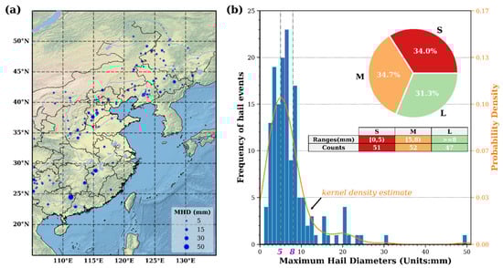
Figure 1.
Distribution of hail events in this study: (a) The geographical spread of 150 hail events (blue dots) in the study region (15°–55°N, 105°–135°E). The sizes of dots represent observed maximum hail diameters (MHDs). The relief map is obtained from Natural Earth I with Shaded Relief and Water (1:10 m). (b) The histogram shows the frequency distribution of hail events with different MHDs. The curve displays the kernel density estimation of the histogram. The two dash-dot lines define the ranges of three size bins: S (), M (), and L ( ). The pie chart and table reveal the percentage and number of S-, M-, and L-size bins, respectively.
ERA5 reanalysis data are employed to calculate the environmental parameters (see Table 1). ERA5 is the fifth generation of the European Centre for Medium-Range Weather Forecasts (ECMWF) atmospheric reanalysis designed to replace ERA-Interim [71]. The ERA5 is run by ECMWF’s Integrated Forecasting System (IFS cycle 41r2) with new and reprocessed observation datasets at a much higher resolution (31 km) and provides an hourly analysis cycle. The involved physical variables in calculating environmental parameters are listed in Table 2. The environmental parameters are calculated with vertical profiles of these quantities.

Table 1.
List of environmental parameters.
Table 2.
ERA5 physical variables that are used to calculate environmental parameters.
FY-4A satellite image data are adopted to calculate hailstorms’ cloud-top parameters (see Table 3). FY-4A is a new generation of Chinese geostationary meteorological satellite launched on 11 December 2016, and positioned at 99.5°E (it drifted to 104.7°E on 25 May 2017) above the equator. The advanced geosynchronous radiation imager (AGRI) of FY-4A has 14 channels, containing 6 visible/near-infrared, 2 mid-infrared, and 6 infrared channels. However, only six infrared channels centered at 6.25, 7.10, 8.50, 10.8, 12.0, and 13.5 μm are accepted the data for consistency between day and night. The spatial resolution of these channels is 4 km at the sub-satellite point. Therefore, the China regional image data are adopted because they have a higher temporal resolution (~5 min) than the full-disk images (~15 min).
Table 3.
List of cloud-top parameters.
2.2. Method
Three steps from satellite and ERA5 data establish the machine learning model for MHDs estimation (see Figure 2):
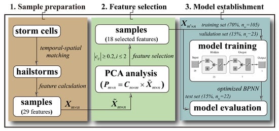
Figure 2.
The flow chart of building MHD estimation model: (1) Step 1: sample preparation; is the sample matrix with all features, where and are the number of features and samples, respectively. (2) Step 2: feature selection; is centered and standardized, is the principal component matrix, and is the coefficient matrix; is the element representing the coefficient of th feature on th PC. (3) Step 3: model establishment; is the sample matrix with selected features and is divided into training (70%, ), validation (15%, ), and test (15%, ) sets for model training and evaluation; a two-layer BPNN regression model with 35 hidden and 1 output units is optimized.
- Sample preparation: This step calculates hailstorms’ environmental and cloud-top parameters to serve as sample features. First, we identify storms on the satellite images with an approach introduced by Liu et al. [106]. Their method can effectively reduce the impact of the anvil clouds. Second, the closest storm to an observed hail event in time and space is marked as a hailstorm. Moreover, the time interval between the storm and hail event should be less than 5 min (satellite time resolution), and the storm should be within 20 km (~5 satellite pixels) from the hail event location. The MHD of the hail event will be assigned to the matched hailstorm. The largest MHD will be accepted if more than one hail event matches the same storm. Third, each pixel or grid’s environmental and cloud-top parameters within the hailstorm boundary are calculated with FY-4A satellite or ERA5 reanalysis data. The final parameters of the hailstorm are the average of all grid or pixel values. Figure 3 demonstrates a hailstorm sample at 09:53 (UTC) on June 6th, 2018. After this step, we obtain 150 hailstorm samples, each of which has 29 features. The original sample set is recorded as , where and represent the number of features and samples, respectively. is a row vector composed of th feature values of all samples.
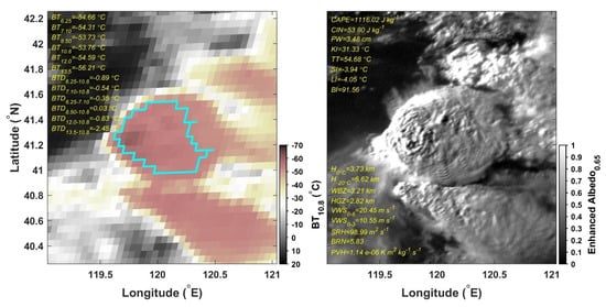 Figure 3. The satellite images showed a hailstorm sample at 09:53 (UTC) on 6 June 2018. The left image is the 10.8 μm channel image, and the cyan polygon draws the identified boundary of the hailstorm. The right image is the 0.65 μm channel image which is enhanced to display the texture of the cloud top. The yellow texts in both images record the 29 features of this hailstorm sample.
 - Feature selection: This step employed a PCA technique [107,108] to select appropriate features to train the machine learning model. The input to PCA is the matrix , where , and , representing the mean and variance of . After PCA calculation, the output is the principal component matrix:where is the coefficient matrix and is the element. The percentage of total variance explained by each principal component (PC) descends from to . The first two PCs explain more than half of the variance, so only is used to select features. As shown in Equation (1), a PC is a linear combination of feature vectors, and the coefficient of each feature vector represents its contribution to the PC. The larger magnitude of the coefficient is, the more significant contribution of the feature vector could make. Thus, we can select features that differ among hail samples by checking whether they have a larger magnitude of coefficients or not. is the applicable criteria of this study, where is the absolute value of , 0.2 is about two-thirds of the coefficients’ magnitude range. Since the hail samples have different MHDs, it inferred that the relations of hail sizes with the selected features are closer than those of the unselected ones.
- Model establishment: This step trains a regression BPNN model with selected features of hail samples and their corresponding MHDs. At first, the sample set (, where is the number of selected features) is randomly divided into three subsets: training, validation, and test by ratios of 0.7, 0.15, and 0.15. The sample sizes of training (), validation (), and test () sets are 105, 23, and 22, individually. Then, the training and validation sets are utilized for training a two-layer BPNN model (see Figure 2). The training set is input to the BPNN, and the associated target outputs are the corresponding MHDs. Levenberg–Marquardt optimization [109] updates the weight and bias values. The active functions of the hidden and output layer are sigmoid and linear, respectively. The mean square error function measures the loss. We try the hidden layer size from 20 to 50 with an interval of 5, and it proves that the size of 35 has the best performance on the validation set . The validation set also makes the training stop early if the network performance fails to improve for 42 epochs. After the BPNN model optimization, the test set is utilized to evaluate the performance of the obtained model on new data. In Section 4.1, the linear fitting contrasts the targeted MHDs and predicted MHDs.
3. Results of PCA-Based Feature Selection
3.1. The Selected Features
Table 4 lists the coefficients of features on the first two PCs. The bolded features are selected (18 in total). Most of them in the () column are cloud-top (environmental) parameters. Noticeably, this reveals that the first and the second PCs focus on two distinct aspects of hailstorm characteristics. Figure 4 illustrates these results by a biplot [108] whose x-axis (y-axis) represents the coefficient values of the first (second) PC. Each line segment from the origin depicts one feature. The x- (y-) axis projection corresponds to the feature’s coefficient on the first (second) PC. In Figure 4, the line segments of selected features extend outside the dashed box, while the unselected features do not.
Table 4.
Feature coefficients for the first ( ) and second ( ) principal components (PCs). The bold fonts mark out the features and coefficients whose magnitudes are greater than 0.2.
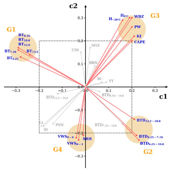
Figure 4.
Biplot graph whose c1-axis and c2-axis represent the first and second PC coefficients. The projection on the c1-axis (c2-axis) reflects the magnitude and sign of each feature’s first (second) PC coefficient. The dotted box divides the selected and unselected features into two areas, where the vectors of selected (unselected) features are outside (inside) the box. Four yellow circular patches present four groups of selected features: G1 (BT group), G2 (BTD group), G3 (thermodynamic group), and G4 (dynamic group).
Moreover, the features with adjacent orientation form the natural groups in Figure 4. Therefore, there are four groups within the selected features: (1) BT group (denoted as G1) including features groups BT8.50, BT10.8, BT12.0, BT6.25, BT7.10, and BT13.5; (2) BTD group (denoted as G2) including BTD6.25−10.8, BTD6.25−7.10, and BTD13.5−10.8; (3) thermodynamic group (denoted as G3) containing CAPE, KI, PW, H0°C, H−20°C, and WBZ; (4) dynamic group (denoted as G4) containing VWS0–3, VWS0–6, and SRH. Next, we demonstrate the feature changes in the four groups with hail sizes and discuss their relations.
3.2. Feature Change with Hail Sizes
Figure 5 is the box plots of selected features in different hail-sized bins (S, M, and L). Figure 5a–d display the results of G1–G4 separately.
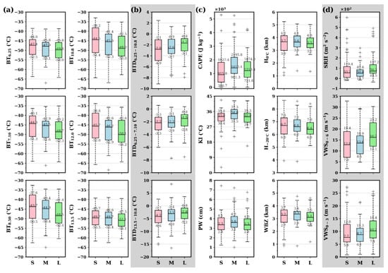
Figure 5.
Box and whisker plots of the selected features for S- (red), M- (blue), and L- (green) size bins: (a) brightness temperature (BT), (b) the difference in BT (BTD), (c) thermodynamic, and (d) dynamic features. Each box’s bottom and top edge represent the 25th and 75th percentile, while the central line shows the median value (50th percentile). Plus signs mark the outliers whose values are more than 1.5 times the distance between the bottom and top edge. The upper (lower) whisker extends to the highest (lowest) datum without considering outliers. The digits in the bottom, middle, and top of each box denote the 25th, 50th, and 75th percentile values of the data set in each size bin, respectively.
In Figure 5a, BT features decrease from the S- to L-size bin, suggesting denser and higher clouds produce larger hailstones. In Figure 5b, the BTD6.25−10.8 and BTD6.25−7.10 of the L-size bin are much larger than the S- and M-size bins, implying that they are helpful for large hail recognition. However, for BTD13.5−10.8, the difference between the S- and M-size bins is more prominent, suggesting this BTD is beneficial for distinguishing small hail from other forms of hail. This is because the peak of the weighting function of the 13.5 μm channel is near the Earth’s surface, which allows the 13.5 μm channel to detect radiation from the lower troposphere. At the same time, the upper water vapor will absorb the low-level radiation in the 6.25 and 7.10 μm channels. Thus, BT6.25 and BT7.10 remain unchanged unless the cloud top reaches peak weighting function levels (~350 and 490 hPa).
In Figure 5c, CAPE and KI are not linearly correlated to hail size, and the L-size bin does not have the maximum CAPE and KI. The residence time of embryos in the growth region of storms should be sufficiently extended to produce large hailstones. Thus, a balance between hailstone fall speed and updraft speed is necessary [110,111,112,113]. If the updraft is too strong, the particles are lofted too quickly to grow to full size and are ejected into the anvil; however, the particles may fall out of the growing region if it is too weak. This may be a partial reason for the L-size bin not having an enormous CAPE and KI. In addition to unstable energy, freezing and melting processes also influence hail size. The L-size bin has the lowest H0°C, H−20°C, and WBZ. The low melting level prevents the hailstones from losing a substantial mass before reaching the ground. On the other hand, the low H−20°C facilitates big drops freezing. Abundant water vapor is necessary for severe convective weather, so the medians of PW for S-, M-, and L-size bins all exceed 3 cm. However, they do not increase with hail size, suggesting that water vapor is not limited to larger hailstones [57].
In Figure 5d, dynamic group features (i.e., shear features VWS0–3, VWS0–6, and SRH) show the most apparent differences between L-size and smaller sized bins compared with other groups in Figure 5a–c. The 25th percentiles of VWS0–3, VWS0–6, and SRH of the L-size bin are larger than or equal to the median values of S- and M-size bins. This suggests that a robust vertical shear environment is necessary for large hail occurrences. As Brooks [45] mentions, given their occurrence, the intensity of tornadoes and hail is entirely a function of shear and only weakly depends on thermodynamic features. The increased VWS can elongate a storm’s updraft, so hail process volumes and hailstone residence times increase and create a vast embryo source region [114].
We also compared the box plots of the unselected features with Figure 5. Their medians fluctuate more gently, and boxes overlap more between S-, M-, and L-size bins. This reflects a stronger correlation of features selected with hail size. However, this relationship is somewhat complicated. For example, hail size positively correlates with cloud-top height, but overlapping BTs generating hailstones are unknown. Although the BTD6.25−10.8 and BTD6.25−7.10 are useful for identifying large hailstones, their ability to distinguish between middle and small hail is weak for lack of low-level information. The dynamic features show better differentiation than thermodynamic features in hail size, especially in relation to larger hail occurrences. Nevertheless, for more acceptable discrimination, it is essential to couple dynamic features with thermodynamic features, which will not be an easy job in terms of the results presented thus far. As a result, we trained a BPNN regression model to predict MHDs by its powerful fitting ability with selected features, and the next section exhibits our results.
4. Model Evaluation
4.1. Comparison between the Observed and Predicted MHD
After building the BPNN model, the predicted MHD is represented as a function of the observed MHD on the test set; we then perform linear fitting (Figure 6). R2 = 0.52 signifies that our model performs well compared with other hail size estimation models. Table 5 compares data, methods, and results between those models at length. Because a linear active function is employed on the output layer of BPNN (see Figure 2), four cases are estimated negative hail size by our model, as seen in Figure 6. The BPNN architecture can be updated to suppress those unphysical results by changing the active function to a positive linear one in future work.
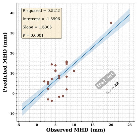
Figure 6.
Linear fitting of predicted vs. observed MHDs on the test set. The sample size is 22 (). The text box at the top left displays the R-squared, the intercept (Intercept) and slope (Slope) values, and the P-value that indicates the confidence interval is 95%.
Table 5.
Comparisons of data, methods, and R-squared on the test set between different maximum hail diameter (MHD) estimation models.
Then, four plots [115] serve to analyze the residuals for a complete diagnosis of the fit. Figure 7a plots “residuals vs. fitted” and shows whether the linear fitting model is reasonable. According to the points distributed along the zero line (gray horizontal dashed line), the trend of the smoothed curve (red line) is flat and close to the zero line, suggesting that there is no distinguished pattern. Figure 7b is a typical Q-Q plot of the residuals utilized to evaluate whether the errors are distributed normally. If the residuals show accurate normal distribution, they will lie precisely on the 45° line (dashed line). It can be seen that the points lie close to the dashed line, demonstrating a slight deviation and an acceptable fit. Figure 7c is a scale–location plot employed to check whether the data are homoscedastic. Its x-axis is identical to Figure 7a, and its y-axis is the standardized residuals’ square root; thus, this plot eliminates the sign of residuals, with a larger magnitude of residuals (positive or negative) plotting the top and small plotting the bottom. We can see that the smoothed curve (red line) is also flat, which means the data are homoscedastic. Figure 7d is an influence plot to show data points that heavily influence the regression line. The influence is measured with Cook’s distance (size of points), which is increased by the leverage (x-axis) and the larger magnitude of residuals (y-axis). The highly influential points are those with Cook’s distance larger than five times the mean Cook’s distance. There is only one in Figure 7d, the data point “21”. This outlier does not have extreme residual but has very large leverage. The leverage measures the influence on the regression due to the location in the variable space. The points that lie far from the centroid or isolate have high leverage. The results reflect a few samples with MHD > 10 mm in Figure 6, and we will add more large MHD samples in future work.
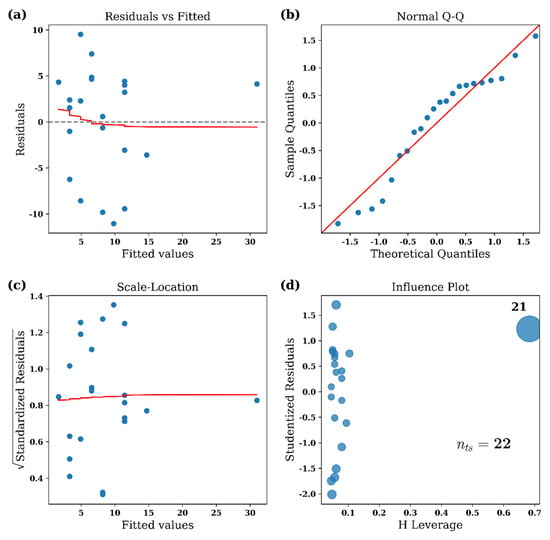
Figure 7.
Diagnosis of linear fitting in Figure 6: (a) the residuals (the vertical distance from a point to the fitted line) vs. fitted values (y-value on the line corresponding to each x-value); (b) normal Q-Q plot of the residuals; if residuals are normally distributed, data points will lie close to the 45° line (red line); (c) square root of the standardized residuals vs. fitted values; (d) studentized residuals vs. leverage; the point size reflects the Cook’s distance which measures how much each data point influences the regression and increases with leverage and large residuals; the numbered points (the digit is the sequence number starting from 0 in the test set; the larger the MHD is, the bigger the digit is) are those that have a significant influence on the fit. The red lines in (a) and (c) are smoothed curves that pass through the actual residuals.
4.2. Case Studies
This section applies the model to all three hail cases from 2019 to 2021 in Shanghai, China. Figure 8, Figure 9 and Figure 10 demonstrate the 500 hPa weather map, SkewT plot, radar reflectivity image, and 10.8 μm satellite image of hail events (marked by the red cross) that occurred in Chongming (2021-4-30 13:14 UTC), Fengxian (2021-5-14 12:30 UTC), and Songjiang (2019-8-18 06:57 UTC) Districts. The observed diameters of hailstones are ~11, 20–30, and 5–10 mm, respectively.
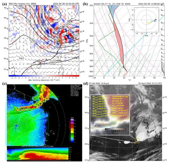
Figure 8.
Hail event (red cross) occurred at about 13:14 (UTC) on 30 April 2021, in Chongming District, Shanghai, China: (a) 500 hPa weather map; (b) SkewT near hail event; (c) radar reflectivity; (d) FY-4A 10.8 μm image, the inset image shows the hailstorm sample (Figure 3a) that was to calculate MHD. The yellow rectangles in (a,d) represent the same geographic range.
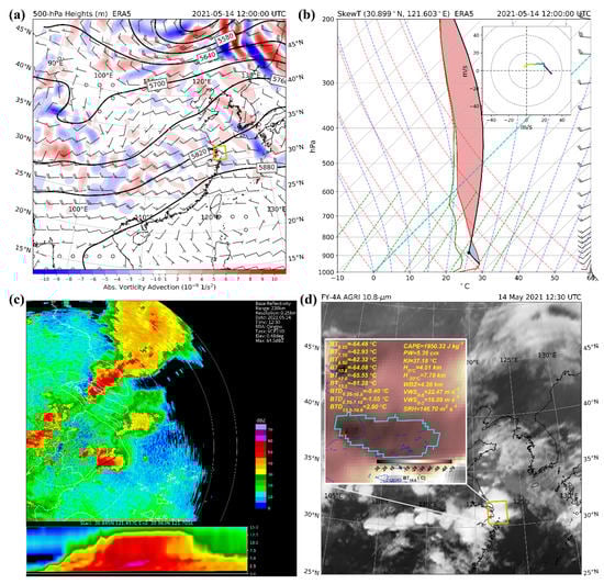
Figure 9.
Hail event (red cross) occurred at about 12:30 (UTC) on 14 May 2021, in Fengxian District, Shanghai, China: (a) 500 hPa weather map; (b) SkewT near hail event; (c) radar reflectivity; (d) FY-4A 10.8 μm image, the inset image shows the hailstorm sample (Figure 3a) that was to calculate MHD. The yellow rectangles in (a,d) represent the same geographic range.
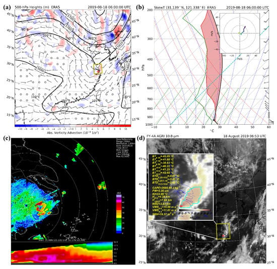
Figure 10.
Hail event (red cross) occurred at about 06:57 (UTC) on 18 August 2019, in Songjiang District, Shanghai, China: (a) 500 hPa weather map; (b) SkewT near hail event; (c) radar reflectivity; (d) FY-4A 10.8 μm image, the inset image shows the hailstorm sample (Figure 3a) that was to calculate MHD. The yellow rectangles in (a,d) represent the same geographic range.
The Chongming hail event is mainly affected by a short-wave trough at the southern periphery of an upper-level cold vortex (Figure 8a). The strong cold advection and the positive vorticity advection at 500 hPa result in the lifting of low-level air and high convective instability in this region. The sounding near the hail event has a relatively dry midlevel layer over a warm and moist low-level layer (Figure 8b), which is conducive to large hailstones reaching the surface and severe and convective local weather [25]. The sounding is characterized by strong VWS, with northerly to northwesterly winds below 850 hPa and westerly winds within the layers above. For the Fengxian hail event, convective cells initiate in front of the 500 hPa short-wave trough and the edge of the 588 line of a subtropical high (Figure 9a), accompanied by a low-level shear line (not shown) that enhances the low-level convergence. The southwesterly low-level jets provide favorable dynamic conditions for this event by transporting warm and moist air to destabilize the environment. The sounding in Figure 9b indicates a conducive environment for this hail event with a strong VWS and a large CAPE. As the convective instability began to increase, the convective cells developed into a long-lasting, heavy storm under the effect of strong VWS. The synoptic patterns associated with the Songjiang hail event are shown in Figure 10a. For this event, the eastern coastal regions of China were beneath a deep upper-level trough. Shanghai is located ahead of the trough and at the southern periphery of the low-level shear line at 850 hPa (not shown), where favorable positive vorticity advection from the trough and low-level convergence near the shear line work together to destabilize the environment. The whole sounding near the hail event is relatively moist (Figure 10b), coupled with an enormous CAPE, conducive to developing organized, deep convection.
The bottoms of Figure 8c, Figure 9c and Figure 10c illustrate the cross-sections of radar echo from which vertical reflectivity distributions are exhibited. The 50 dBz echo tops are about 7, 12, and 10 km in the Chongming, Fengxian, and Songjiang cases, while the ≥ 60 dBz echo region in the Songjiang case is the most extensive. We calculated the MEHS from radar reflectivity with the method used in Witt et al. [24]. Being different from the machine learning method, MEHS are obtained from an empirical equation that weights radar reflectivity from 0 °C level through −20 °C level to echo top:
where is flux value of hail kinetic energy that is transformed from reflectivity data, is the height above radar level (ARL), is the temperature-based weighting function that suggests hail growth which only occurs below 0 °C and mainly occurs at temperatures near −20 °C or colder, is the height ARL of melting level, and is the height of storm top. Please refer to Witt et al. [24] for more details. The calculated MEHS are about 30, 53, and 61 mm for the Chongming, Fengxian, and Songjiang cases, which are much larger than the observed diameters (~11, 20–30, and 5–10 mm) and not quite reasonable according to the statistics of hail size in China where severe hail events (MHD ≥ 30 mm) are rare [57]. These indicate that MEHS estimation cannot be directly adopted outside the region developed before localization.
Figure 8d, Figure 9d and Figure 10d demonstrate the large-scale clouds corresponding to weather systems and atmospheric physical processes displayed in Figure 8a, Figure 9a and Figure 10a. A vortex cloud system in the upper section of Figure 8d and a leafy cloud system at the bottom left of Figure 10d are associated with the northeastern cold vortex and trough in Figure 8a and Figure 9a, respectively. Figure 9d shows a shear-line cloud band composed of convective clouds located at the periphery of the subtropical high. The inset images of Figure 8d, Figure 9d and Figure 10d illustrate hailstorms in detail and list the input features of the BPNN model. Eventually, the estimated MHDs by the BPNN model are about 12, 25, and 9 mm in the Chongming, Fengxian, and Songjiang cases, which are all close to the observations (~11, 20–30, and 5–10 mm). We also compare environmental and cloud-top features of hailstorms among three cases and find their change with hail size follows the rules obtained in Section 3.2. With the largest hail size, the Fengxian case has the highest cloud top and maximum VWS. The Chongming case has a similar VWS to the Fengxian case, but it has a lower cloud top than the latter, and its hail size is smaller. The Songjiang case has the smallest VWS and the lowest cloud top, and its hailstone size is the smallest. Additionally, the CAPE of the Songjiang case is the largest, the Fengxian case is the second largest, and the Chongming case is the smallest. These results suggest that the cloud-top and dynamic features have a stronger positive correlation with hail size. In contrast, thermodynamic features are not limited to hail size as long as the energy is sufficient for hail occurrence. In any event, hail size results from multiple factors and is difficult to judge by only one.
5. Discussions
Some hailstorms produce giant hailstones while others produce smaller hailstones; however, the reasons for these discrepancies are not yet fully understood [16]. Consequently, it is helpful to indirectly evaluate hailstone sizes from satellites that provide continuous, extensive, and early storm observations coupled with sounding data to add vertical atmospheric information to cloud-top characteristics. The objective selection of environmental and cloud-top features based on PCA is implemented in China and can be immediately extended to other regions conveniently. Furthermore, this method is also available when selecting new variables, such as new satellite channels or new weather phenomena recognition, e.g., heavy rainfall, strong wind.
One difficulty in hail size diagnoses is that relations in one region may not quickly transfer to another area. However, the data-driven machine learning method without necessary equation assumptions in advance proves a promising solution. Another difficulty is a lack of accurate, dense, and full hail observations. Clearly, more hail samples with a wide size distribution for training, validation, and testing can improve BPNN model robustness. Additionally, more case studies in different geographical areas and seasons are helpful before its usage. Nevertheless, with more and better meteorological observations planned for the future, the machine learning model will prove an adequate approach for predicting hailstone size.
6. Conclusions
This study established a hail size estimation model from satellite images based on two algorithms, PCA and BPNN.
The PCA-based technique selects features closely related to hail sizes from 29 candidate parameters. These parameters contain wind shear, temperature layer, instability energy, water vapor, cloud-top height, cloud thickness, cloud-top phase, etc. As a result, a total of 18 features were strictly and carefully selected according to PC contribution and parameter coefficients. Those features naturally congregated into four groups: BT (BT6.25, BT7.10, BT8.50, BT10.8, BT12.0, BT13.5), BTD (BTD6.25−10.8, BTD6.25−7.10, BTD13.5−10.8), thermodynamic (CAPE, KI, PW, H0°C, H−20°C, WBZ), and dynamic (VWS0–3, VWS0–6, SRH) groups. The statistics of the four group features for different hail-sized bins demonstrate that hailstorms with a higher cloud-top height and denser clouds produce larger hailstones. The largest hailstones occur in an environment with strong vertical wind shear and a low melting/freezing level height. Abundant moisture supply and instability energy are required for hail occurrence but are not limiting factors for the largest hailstones. Although the selected features vary more apparently with hail sizes than the unselected ones, the relations between these features and hail size are complicated and nonlinear. As a result, the machine learning model BPNN, with powerful fitting ability, is adopted to estimate hailstone size.
Next, to establish the BPNN regression model, the hail samples were segregated into training (70%), validation (15%), and test (15%) sets. The training set trains the BPNN model; the validation set checks the model during training and decides when to stop training early; the test set estimates model accuracy in new data. The BPNN regression model has a two-layer architecture with 35 hidden layer neurons and a mean squared error loss function. The linear fitting R2 between predicted and observed MHDs on the test set is 0.52. In the Shanghai case studies, the prediction of MHD is close to the observed value and is more reasonable than the MEHS results, which overestimate hail size. All of the results suggest that this model can be applied in practice.
Author Contributions
Conceptualization, Q.W., Y.-X.S., L.-M.M. and Q.L.; Data curation, Q.W. and Y.-X.S.; Formal analysis, Q.W.; Funding acquisition, Q.W. and L.-M.M.; Investigation, Q.W., L.-M.M. and R.W.; Methodology, Q.W.; Resources, Y.-X.S., L.-M.M. and Q.L.; Validation, Q.W.; Visualization, Q.W.; Writing—original draft, Q.W. and R.W.; Writing—review & editing, Q.W., Y.-X.S. and L.-M.M. All authors have read and agreed to the published version of the manuscript.
Funding
This research was sponsored by the National Natural Science Foundation of China (No. 42005111 and No. 41975069), Shanghai Sailing Program (No. 20YF1449200).
Acknowledgments
The FY-4A AGRI L1 data are obtained from the National Satellite Meteorological Center (NSMC) of CMA (http://satellite.nsmc.org.cn/PortalSite/Default.aspx; Accessed between 2018 and 2021). The ERA5 data are downloaded from the Climate Data Store (CDS, https://cds.climate.copernicus.eu/cdsapp#!/home). The hail event records are collected from the NMIC of CMA. The shaded relief and water map data are obtained from Natural Earth (https://www.naturalearthdata.com/downloads/10m-natural-earth-1/10m-natural-earth-1-with-shaded-relief-and-water/; Accessed 9 December 2020). We thank them all for their excellent data collection and production work.
Conflicts of Interest
The authors declare no conflict of interest.
References
- Knight, C.A.; Knight, N.C. Very Large Hailstones From Aurora, Nebraska. Bull. Am. Meteorol. Soc. 2005, 86, 1773–1782. [Google Scholar] [CrossRef]
- Kumjian, M.R.; Lebo, Z.J.; Ward, A.M. Storms Producing Large Accumulations of Small Hail. J. Appl. Meteorol. Climatol. 2019, 58, 341–364. [Google Scholar] [CrossRef]
- Mahoney, K.; Alexander, M.A.; Thompson, G.; Barsugli, J.J.; Scott, J.D. Changes in hail and flood risk in high-resolution simulations over Colorado’s mountains. Nat. Clim. Chang. 2012, 2, 125–131. [Google Scholar] [CrossRef]
- Allen, J.T.; Tippett, M.K. The Characteristics of United States Hail Reports: 1955–2014. E-J. Sev. Storms Meteorol. 2015, 10, 1–31. [Google Scholar]
- Allen, J.T. Hail potential heating up. Nat. Clim. Chang. 2017, 7, 474–475. [Google Scholar] [CrossRef]
- Brimelow, J.C.; Burrows, W.R.; Hanesiak, J.M. The changing hail threat over North America in response to anthropogenic climate change. Nat. Clim. Chang. 2017, 7, 516–522. [Google Scholar] [CrossRef]
- Trapp, R.J.; Hoogewind, K.A.; Lasher-Trapp, S. Future Changes in Hail Occurrence in the United States Determined through Convection-Permitting Dynamical Downscaling. J. Clim. 2019, 32, 5493–5509. [Google Scholar] [CrossRef]
- Raupach, T.H.; Martius, O.; Allen, J.T.; Kunz, M.; Lasher-Trapp, S.; Mohr, S.; Rasmussen, K.L.; Trapp, R.J.; Zhang, Q. The effects of climate change on hailstorms. Nat. Rev. Earth Environ. 2021, 2, 213–226. [Google Scholar] [CrossRef]
- Brown, T.M.; Pogorzelski, W.H.; Giammanco, I.M. Evaluating Hail Damage Using Property Insurance Claims Data. Weather Clim. Soc. 2015, 7, 197–210. [Google Scholar] [CrossRef]
- Punge, H.J.; Bedka, K.M.; Kunz, M.; Werner, A. A new physically based stochastic event catalog for hail in Europe. Nat. Hazards 2014, 73, 1625–1645. [Google Scholar] [CrossRef]
- Grieser, J.; Hill, M. How to Express Hail Intensity—Modeling the Hailstone Size Distribution. J. Appl. Meteorol. Climatol. 2019, 58, 2329–2345. [Google Scholar] [CrossRef]
- Webb, J.D.C.; Elsom, D.M.; Reynolds, D.J. Climatology of severe hailstorms in Great Britain. Atmos. Res. 2001, 56, 291–308. [Google Scholar] [CrossRef]
- Dessens, J.; Berthet, C.; Sanchez, J.L. A point hailfall classification based on hailpad measurements: The ANELFA scale. Atmos. Res. 2007, 83, 132–139. [Google Scholar] [CrossRef]
- Hohl, R.; Schiesser, H.-H.; Knepper, I. The use of weather radars to estimate hail damage to automobiles: An exploratory study in Switzerland. Atmos. Res. 2002, 61, 215–238. [Google Scholar] [CrossRef]
- Hohl, R.; Schiesser, H.-H.; Aller, D. Hailfall: The relationship between radar-derived hail kinetic energy and hail damage to buildings. Atmos. Res. 2002, 63, 177–207. [Google Scholar] [CrossRef]
- Allen, J.T.; Giammanco, I.M.; Kumjian, M.R.; Jurgen Punge, H.; Zhang, Q.; Groenemeijer, P.; Kunz, M.; Ortega, K. Understanding Hail in the Earth System. Rev. Geophys. 2020, 58, e2019RG000665. [Google Scholar] [CrossRef]
- Punge, H.J.; Kunz, M. Hail observations and hailstorm characteristics in Europe: A review. Atmos. Res. 2016, 176–177, 159–184. [Google Scholar] [CrossRef]
- Martius, O.; Hering, A.; Kunz, M.; Manzato, A.; Mohr, S.; Nisi, L.; Trefalt, S. Challenges and Recent Advances in Hail Research. Bull. Am. Meteorol. Soc. 2018, 99, ES51–ES54. [Google Scholar] [CrossRef]
- Cintineo, J.L.; Smith, T.M.; Lakshmanan, V.; Brooks, H.E.; Ortega, K.L. An Objective High-Resolution Hail Climatology of the Contiguous United States. Weather Forecast. 2012, 27, 1235–1248. [Google Scholar] [CrossRef]
- Kunz, M.; Kugel, P.I.S. Detection of hail signatures from single-polarization C-band radar reflectivity. Atmos. Res. 2015, 153, 565–577. [Google Scholar] [CrossRef]
- Ortega, K.L.; Krause, J.M.; Ryzhkov, A.V. Polarimetric Radar Characteristics of Melting Hail. Part III: Validation of the Algorithm for Hail Size Discrimination. J. Appl. Meteorol. Climatol. 2016, 55, 829–848. [Google Scholar] [CrossRef]
- Wang, P.; Shi, J.; Hou, J.; Hu, Y. The Identification of Hail Storms in the Early Stage Using Time Series Analysis. J. Geophys. Res. Atmos. 2018, 123, 929–947. [Google Scholar] [CrossRef]
- Czernecki, B.; Taszarek, M.; Marosz, M.; Półrolniczak, M.; Kolendowicz, L.; Wyszogrodzki, A.; Szturc, J. Application of machine learning to large hail prediction—The importance of radar reflectivity, lightning occurrence and convective parameters derived from ERA5. Atmos. Res. 2019, 227, 249–262. [Google Scholar] [CrossRef]
- Witt, A.; Eilts, M.D.; Stumpf, G.J.; Johnson, J.T.; Mitchell, E.D.W.; Thomas, K.W. An Enhanced Hail Detection Algorithm for the WSR-88D. Weather Forecast. 1998, 13, 286–303. [Google Scholar] [CrossRef]
- Luo, L.; Xue, M.; Zhu, K.; Zhou, B. Explicit Prediction of Hail in a Long-Lasting Multicellular Convective System in Eastern China Using Multimoment Microphysics Schemes. J. Atmos. Sci. 2018, 75, 3115–3137. [Google Scholar] [CrossRef]
- Nisi, L.; Hering, A.; Germann, U.; Martius, O. A 15-year hail streak climatology for the Alpine region. Q. J. R. Meteorol. Soc. 2018, 144, 1429–1449. [Google Scholar] [CrossRef]
- Ortega, K.L. Evaluating multi-radar, multi-sensor products for surface hailfall diagnosis. E-J. Sev. Storms Meteorol. 2018, 13, 1–36. [Google Scholar]
- Lee, S.; Han, H.; Im, J.; Jang, E.; Lee, M.I. Detection of deterministic and probabilistic convection initiation using Himawari-8 Advanced Himawari Imager data. Atmos. Meas. Tech. 2017, 10, 1859–1874. [Google Scholar] [CrossRef]
- Liu, Z.; Min, M.; Li, J.; Sun, F.; Di, D.; Ai, Y.; Li, Z.; Qin, D.; Li, G.; Lin, Y.; et al. Local Severe Storm Tracking and Warning in Pre-Convection Stage from the New Generation Geostationary Weather Satellite Measurements. Remote Sens. 2019, 11, 383. [Google Scholar] [CrossRef]
- Sun, F.; Qin, D.; Min, M.; Li, B.; Wang, F. Convective Initiation Nowcasting Over China from Fengyun-4A Measurements Based on TV-L1 Optical Flow and BP_Adaboost Neural Network Algorithms. IEEE J. Sel. Top. Appl. Earth Obs. Remote Sens. 2019, 12, 4284–4296. [Google Scholar] [CrossRef]
- Cintineo, J.L.; Pavolonis, M.J.; Sieglaff, J.M.; Wimmers, A.; Brunner, J.; Bellon, W. A Deep-Learning Model for Automated Detection of Intense Midlatitude Convection Using Geostationary Satellite Images. Weather Forecast. 2020, 35, 2567–2588. [Google Scholar] [CrossRef]
- Li, W.; Zhang, F.; Yu, Y.; Iwabuchi, H.; Shen, Z.; Wang, G.; Zhang, Y. The semi-diurnal cycle of deep convective systems over Eastern China and its surrounding seas in summer based on an automatic tracking algorithm. Clim. Dyn. 2021, 56, 357–379. [Google Scholar] [CrossRef]
- Kuligowski, R.J.; Li, Y.; Hao, Y.; Zhang, Y. Improvements to the GOES-R Rainfall Rate Algorithm. J. Hydrometeorol. 2016, 17, 1693–1704. [Google Scholar] [CrossRef]
- Beusch, L.; Foresti, L.; Gabella, M.; Hamann, U. Satellite-Based Rainfall Retrieval: From Generalized Linear Models to Artificial Neural Networks. Remote Sens. 2018, 10, 939. [Google Scholar] [CrossRef]
- Lee, Y.; Han, D.; Ahn, M.-H.; Im, J.; Lee, S.J. Retrieval of Total Precipitable Water from Himawari-8 AHI Data: A Comparison of Random Forest, Extreme Gradient Boosting, and Deep Neural Network. Remote Sens. 2019, 11, 1741. [Google Scholar] [CrossRef]
- Chen, Z.; Yu, X. A Novel Tensor Network for Tropical Cyclone Intensity Estimation. IEEE Trans. Geosci. Remote Sens. 2021, 59, 3226–3243. [Google Scholar] [CrossRef]
- Zhang, C.J.; Wang, X.J.; Ma, L.M.; Lu, X.Q. Tropical Cyclone Intensity Classification and Estimation Using Infrared Satellite Images with Deep Learning. IEEE J. Sel. Top. Appl. Earth Obs. Remote Sens. 2021, 14, 2070–2086. [Google Scholar] [CrossRef]
- Merino, A.; López, L.; Sánchez, J.L.; García-Ortega, E.; Cattani, E.; Levizzani, V. Daytime identification of summer hailstorm cells from MSG data. Nat. Hazards Earth Syst. Sci. 2014, 14, 1017–1033. [Google Scholar] [CrossRef]
- Melcón, P.; Merino, A.; Sánchez, J.L.; López, L.; Hermida, L. Satellite remote sensing of hailstorms in France. Atmos. Res. 2016, 182, 221–231. [Google Scholar] [CrossRef]
- Punge, H.J.; Bedka, K.M.; Kunz, M.; Reinbold, A. Hail frequency estimation across Europe based on a combination of overshooting top detections and the ERA-INTERIM reanalysis. Atmos. Res. 2017, 198, 34–43. [Google Scholar] [CrossRef]
- López, L.; Marcos, J.L.; Sánchez, J.L.; Castro, A.; Fraile, R. CAPE values and hailstorms on northwestern Spain. Atmos. Res. 2001, 56, 147–160. [Google Scholar] [CrossRef]
- López, L.; García-Ortega, E.; Sánchez, J.L. A short-term forecast model for hail. Atmos. Res. 2007, 83, 176–184. [Google Scholar] [CrossRef]
- Fraile, R.; Castro, A.; López, L.; Sánchez, J.L.; Palencia, C. The influence of melting on hailstone size distribution. Atmos. Res. 2003, 67–68, 203–213. [Google Scholar] [CrossRef]
- Brooks, H.E. Proximity soundings for severe convection for Europe and the United States from reanalysis data. Atmos. Res. 2009, 93, 546–553. [Google Scholar] [CrossRef]
- Brooks, H.E. Severe thunderstorms and climate change. Atmos. Res. 2013, 123, 129–138. [Google Scholar] [CrossRef]
- Palencia, C.; Giaiotti, D.; Stel, F.; Castro, A.; Fraile, R. Maximum hailstone size: Relationship with meteorological variables. Atmos. Res. 2010, 96, 256–265. [Google Scholar] [CrossRef]
- García-Ortega, E.; Merino, A.; López, L.; Sánchez, J.L. Role of mesoscale factors at the onset of deep convection on hailstorm days and their relation to the synoptic patterns. Atmos. Res. 2012, 114–115, 91–106. [Google Scholar] [CrossRef]
- Eccel, E.; Cau, P.; Riemann-Campe, K.; Biasioli, F. Quantitative hail monitoring in an alpine area: 35-year climatology and links with atmospheric variables. Int. J. Climatol. 2012, 32, 503–517. [Google Scholar] [CrossRef]
- Merino, A.; García-Ortega, E.; López, L.; Sánchez, J.L.; Guerrero-Higueras, A.M. Synoptic environment, mesoscale configurations and forecast parameters for hailstorms in Southwestern Europe. Atmos. Res. 2013, 122, 183–198. [Google Scholar] [CrossRef]
- Mohr, S.; Kunz, M. Recent trends and variabilities of convective parameters relevant for hail events in Germany and Europe. Atmos. Res. 2013, 123, 211–228. [Google Scholar] [CrossRef]
- Zheng, L.; Sun, J.; Zhang, X.; Liu, C. Organizational Modes of Mesoscale Convective Systems over Central East China. Weather Forecast. 2013, 28, 1081–1098. [Google Scholar] [CrossRef]
- Johnson, A.W.; Sugden, K.E. Evaluation of sounding-derived thermodynamic and wind-related parameters associated with large hail events. E-J. Sev. Storms Meteorol. 2014, 9, 1–42. [Google Scholar]
- Gascón, E.; Merino, A.; Sánchez, J.L.; Fernández-González, S.; García-Ortega, E.; López, L.; Hermida, L. Spatial distribution of thermodynamic conditions of severe storms in southwestern Europe. Atmos. Res. 2015, 164–165, 194–209. [Google Scholar] [CrossRef]
- Vujović, D.; Paskota, M.; Todorović, N.; Vučković, V. Evaluation of the stability indices for the thunderstorm forecasting in the region of Belgrade, Serbia. Atmos. Res. 2015, 161–162, 143–152. [Google Scholar] [CrossRef]
- Melcón, P.; Merino, A.; Sánchez, J.L.; López, L.; García-Ortega, E. Spatial patterns of thermodynamic conditions of hailstorms in southwestern France. Atmos. Res. 2017, 189, 111–126. [Google Scholar] [CrossRef]
- Prein, A.F.; Holland, G.J. Global estimates of damaging hail hazard. Weather Clim. Extrem. 2018, 22, 10–23. [Google Scholar] [CrossRef]
- Li, M.; Zhang, D.-L.; Sun, J.; Zhang, Q. A Statistical Analysis of Hail Events and Their Environmental Conditions in China during 2008–2015. J. Appl. Meteorol. Climatol. 2018, 57, 2817–2833. [Google Scholar] [CrossRef]
- Mecikalski, J.R.; MacKenzie, W.M.; König, M.; Muller, S. Cloud-Top Properties of Growing Cumulus prior to Convective Initiation as Measured by Meteosat Second Generation. Part II: Use of Visible Reflectance. J. Appl. Meteorol. Climatol. 2010, 49, 2544–2558. [Google Scholar] [CrossRef]
- Park, M.-S.; Kim, M.; Lee, M.-I.; Im, J.; Park, S. Detection of tropical cyclone genesis via quantitative satellite ocean surface wind pattern and intensity analyses using decision trees. Remote Sens. Environ. 2016, 183, 205–214. [Google Scholar] [CrossRef]
- Yao, H.; Li, X.; Pang, H.; Sheng, L.; Wang, W. Application of random forest algorithm in hail forecasting over Shandong Peninsula. Atmos. Res. 2020, 244, 105093. [Google Scholar] [CrossRef]
- Marzban, C.; Witt, A. A Bayesian Neural Network for Severe-Hail Size Prediction. Weather Forecast. 2001, 16, 600–610. [Google Scholar] [CrossRef]
- Manzato, A. Hail in Northeast Italy: A Neural Network Ensemble Forecast Using Sounding-Derived Indices. Weather Forecast. 2013, 28, 3–28. [Google Scholar] [CrossRef]
- Han, L.; Sun, J.; Zhang, W.; Xiu, Y.; Feng, H.; Lin, Y. A machine learning nowcasting method based on real-time reanalysis data. J. Geophys. Res. Atmos. 2017, 122, 4038–4051. [Google Scholar] [CrossRef]
- Lazri, M.; Labadi, K.; Brucker, J.M.; Ameur, S. Improving satellite rainfall estimation from MSG data in Northern Algeria by using a multi-classifier model based on machine learning. J. Hydrol. 2020, 584, 124705. [Google Scholar] [CrossRef]
- Zhang, J.; Liu, P.; Zhang, F.; Song, Q. CloudNet: Ground-Based Cloud Classification with Deep Convolutional Neural Network. Geophys. Res. Lett. 2018, 45, 8665–8672. [Google Scholar] [CrossRef]
- Shi, X.; Chen, Z.; Wang, H.; Yeung, D.-Y.; Wong, W.-K.; Woo, W.-C. Convolutional LSTM Network: A machine learning approach for precipitation nowcasting. In Proceedings of the Proceedings of the 28th International Conference on Neural Information Processing Systems, Montreal, QC, Canada, 7–12 December 2015; Volume 1, pp. 802–810. [Google Scholar]
- Xiao, H.; Zhang, F.; He, Q.; Liu, P.; Yan, F.; Miao, L.; Yang, Z. Classification of Ice Crystal Habits Observed from Airborne Cloud Particle Imager by Deep Transfer Learning. Earth Space Sci. 2019, 6, 1877–1886. [Google Scholar] [CrossRef]
- Zhou, Z.; Zhang, F.; Xiao, H.; Wang, F.; Hong, X.; Wu, K.; Zhang, J. A Novel Ground-Based Cloud Image Segmentation Method by Using Deep Transfer Learning. IEEE Geosci. Remote Sens. Lett. 2021, 1–5. [Google Scholar] [CrossRef]
- Kim, K.; Kim, J.-H.; Moon, Y.-J.; Park, E.; Shin, G.; Kim, T.; Kim, Y.; Hong, S. Nighttime Reflectance Generation in the Visible Band of Satellites. Remote Sens. 2019, 11, 2087. [Google Scholar] [CrossRef]
- Ni, X.; Zhang, Q.; Liu, C.; Li, X.; Zou, T.; Lin, J.; Kong, H.; Ren, Z. Decreased hail size in China since 1980. Sci. Rep. 2017, 7, 10913. [Google Scholar] [CrossRef]
- Hans, H.; Bell, W.; Berrisford, P.; Andras, H.; Muñoz-Sabater, J.; Nicolas, J.; Raluca, R.; Dinand, S.; Adrian, S.; Cornel, S.; et al. Global reanalysis: Goodbye ERA-Interim, hello ERA5. ECMWF Newsl. 2019, 159, 17–24. [Google Scholar]
- Moncrieff, M.W.; Miller, M.J. The dynamics and simulation of tropical cumulonimbus and squall lines. Q. J. R. Meteorol. Soc. 1976, 102, 373–394. [Google Scholar] [CrossRef]
- Colby, F.P., Jr. Convective inhibition as a predictor of convection during AVE-SESAME II. Mon. Weather Rev. 1984, 112, 2239–2252. [Google Scholar] [CrossRef]
- George, J.J. Weather Forecasting for Aeronautics; Academic Press: San Diego, CA, USA, 1960. [Google Scholar]
- Miller, R. Notes on Analysis and Severe-Storm Forecasting Procedures of the Air Force Global Weather Central; Technical Report 200 (Rev); AWS, U.S. Air Force: Scott AFB, IL, USA, 1972; 102p. [Google Scholar]
- Showalter, A.K. A Stability Index for Thunderstorm Forecasting. Bull. Am. Meteorol. Soc. 1953, 34, 250–252. [Google Scholar] [CrossRef]
- Galway, J.G. The Lifted Index as a Predictor of Latent Instability. Bull. Am. Meteorol. Soc. 1956, 37, 528–529. [Google Scholar] [CrossRef]
- Boyden, C. A simple instability index for use as a synoptic parameter. Meteor. Mag. 1963, 92, 198–210. [Google Scholar]
- Dessens, J.; Berthet, C.; Sanchez, J.L. Change in hailstone size distributions with an increase in the melting level height. Atmos. Res. 2015, 158–159, 245–253. [Google Scholar] [CrossRef]
- Johns, R.H.; Doswell, C.A. Severe Local Storms Forecasting. Weather Forecast. 1992, 7, 588–612. [Google Scholar] [CrossRef]
- Fawbush, E.J.; Miller, R.C. A Method for Forecasting Hailstone Size at the Earth’s Surface. Bull. Am. Meteorol. Soc. 1953, 34, 235–244. [Google Scholar] [CrossRef][Green Version]
- Knight, C.A.; Knight, N.C. Hailstorms. In Severe Convective Storms; Meteorol. Monogr; Doswell, C.A., Ed.; American Meteorological Society: Boston, MA, USA, 2001; Volume 28, pp. 223–248. [Google Scholar]
- Weisman, M.L.; Klemp, J.B. The Dependence of Numerically Simulated Convective Storms on Vertical Wind Shear and Buoyancy. Mon. Weather Rev. 1982, 110, 504–520. [Google Scholar] [CrossRef]
- Weisman, M.L.; Klemp, J.B. Characteristics of Isolated Convective Storms. In Mesoscale Meteorology and Forecasting; Ray, P.S., Ed.; American Meteorological Society: Boston, MA, USA, 1986; pp. 331–358. [Google Scholar]
- Ziegler, C.L.; Ray, P.S.; Knight, N.C. Hail Growth in an Oklahoma Multicell Storm. J. Atmos. Sci. 1983, 40, 1768–1791. [Google Scholar] [CrossRef]
- Tuovinen, J.-P.; Rauhala, J.; Schultz, D.M. Significant-Hail-Producing Storms in Finland: Convective-Storm Environment and Mode. Weather Forecast. 2015, 30, 1064–1076. [Google Scholar] [CrossRef]
- Xie, B.; Zhang, Q.; Wang, Y. Observed Characteristics of Hail Size in Four Regions in China during 1980–2005. J. Clim. 2010, 23, 4973–4982. [Google Scholar] [CrossRef]
- Weisman, M.L.; Klemp, J.B. The structure and classification of numerically simulated convective stormsin directionally varying wind shears. Mon. Weather Rev. 1984, 112, 2479–2498. [Google Scholar] [CrossRef]
- Davies-Jones, R.; Burgess, D.; Foster, M. Test of helicity as a tornado forecast parameter. In Proceedings of the 16th Conference on Severe Local Storms, Kananaskis Provincial Park, AB, Canada, 22–26 October 1990; pp. 107–111. [Google Scholar]
- Maddox, R.A. An Evaluation of Tornado Proximity Wind and Stability Data. Mon. Weather Rev. 1976, 104, 133–142. [Google Scholar] [CrossRef]
- Rossby, C. Planetary flow pattern in the atmosphere. Q. J. R. Meteorol. Soc. 1940, 66, 68–87. [Google Scholar]
- Ertel, H. Ein neuer hydrodynamischer Wirbelsatz. Met. Z. 1942, 59, 277–281. [Google Scholar]
- Hoskins, B.J.; McIntyre, M.E.; Robertson, A.W. On the use and significance of isentropic potential vorticity maps. Q. J. R. Meteorol. Soc. 1985, 111, 877–946. [Google Scholar] [CrossRef]
- Schmetz, J.; Pili, P.; Tjemkes, S.; Just, D.; Kerkmann, J.; Rota, S.; Ratier, A. An Introduction to Meteosat Second Generation (MSG). Bull. Am. Meteorol. Soc. 2002, 83, 977–992. [Google Scholar] [CrossRef]
- Schmit, T.J.; Griffith, P.; Gunshor, M.M.; Daniels, J.M.; Goodman, S.J.; Lebair, W.J. A Closer Look at the ABI on the GOES-R Series. Bull. Am. Meteorol. Soc. 2017, 98, 681–698. [Google Scholar] [CrossRef]
- Yang, J.; Zhang, Z.; Wei, C.; Lu, F.; Guo, Q. Introducing the New Generation of Chinese Geostationary Weather Satellites, Fengyun-4. Bull. Am. Meteorol. Soc. 2017, 98, 1637–1658. [Google Scholar] [CrossRef]
- Zhuge, X.; Zou, X. Summertime convective initiation nowcasting over southeastern China based on Advanced Himawari Imager observations. J. Meteorol. Soc. Jpn. Ser. II 2018, 96, 337–353. [Google Scholar] [CrossRef]
- Mecikalski, J.R.; Bedka, K.M.; Paech, S.J.; Litten, L.A. A Statistical Evaluation of GOES Cloud-Top Properties for Nowcasting Convective Initiation. Mon. Weather Rev. 2008, 136, 4899–4914. [Google Scholar] [CrossRef]
- Ackerman, S.A. Global Satellite Observations of Negative Brightness Temperature Differences between 11 and 6.7 µm. J. Atmos. Sci. 1996, 53, 2803–2812. [Google Scholar] [CrossRef]
- Schmetz, J.; Tjemkes, S.A.; Gube, M.; van de Berg, L. Monitoring deep convection and convective overshooting with METEOSAT. Adv. Space Res. 1997, 19, 433–441. [Google Scholar] [CrossRef]
- Matthee, R.; Mecikalski, J.R. Geostationary infrared methods for detecting lightning-producing cumulonimbus clouds. J. Geophys. Res. Atmos. 2013, 118, 6580–6592. [Google Scholar] [CrossRef]
- Strabala, K.I.; Ackerman, S.A.; Menzel, W.P. Cloud properties inferred from 8–12-µm data. J. Appl. Meteorol. Climatol. 1994, 33, 212–229. [Google Scholar] [CrossRef]
- Ellrod, G.P. Impact on volcanic ash detection caused by the loss of the 12.0 μm “Split Window” band on GOES Imagers. J. Volcanol. Geotherm. Res. 2004, 135, 91–103. [Google Scholar] [CrossRef]
- Mecikalski, J.R.; Bedka, K.M. Forecasting Convective Initiation by Monitoring the Evolution of Moving Cumulus in Daytime GOES Imagery. Mon. Weather Rev. 2006, 134, 49–78. [Google Scholar] [CrossRef]
- Inoue, T. A cloud type classification with NOAA 7 split-window measurements. J. Geophys. Res. Atmos. 1987, 92, 3991–4000. [Google Scholar] [CrossRef]
- Liu, J.; Ma, C.; Liu, C.; Qin, D.; Gu, X. An extended maxima transform-based region growing algorithm for convective cell detection on satellite images. Remote Sens. Lett. 2014, 5, 971–980. [Google Scholar] [CrossRef]
- Jolliffe, I. Principal component analysis for special types of data. In Principal Component Analysis; Springer Series in Statistics; Springer: New York, NY, USA, 2002; pp. 338–372. [Google Scholar] [CrossRef]
- Wilks, D.S. Chapter 13—Principal Component (EOF) Analysis. In Statistical Methods in the Atmospheric Sciences, 4th ed.; Wilks, D.S., Ed.; Elsevier: Amsterdam, The Netherlands, 2019; pp. 617–668. [Google Scholar]
- Marquardt, D.W. An algorithm for least-squares estimation of nonlinear parameters. J. Soc. Ind. Appl. Math. 1963, 11, 431–441. [Google Scholar] [CrossRef]
- Browning, K.A.; Foote, G.B. Airflow and hail growth in supercell storms and some implications for hail suppression. Q. J. R. Meteorol. Soc. 1976, 102, 499–533. [Google Scholar] [CrossRef]
- Heymsfield, A.J. Case Study of a Halistorm in Colorado. Part IV: Graupel and Hail Growth Mechanisms Deduced through Particle Trajectory Calculations. J. Atmos. Sci. 1983, 40, 1482–1509. [Google Scholar] [CrossRef]
- Foote, G.B. A Study of Hail Growth Utilizing Observed Storm Conditions. J. Appl. Meteorol. Climatol. 1984, 23, 84–101. [Google Scholar] [CrossRef]
- Musil, D.J.; Heymsfield, A.J.; Smith, P.L. Microphysical Characteristics of a Well-Developed Weak Echo Region in a High Plains Supercell Thunderstorm. J. Appl. Meteorol. Climatol. 1986, 25, 1037–1051. [Google Scholar] [CrossRef]
- Dennis, E.J.; Kumjian, M.R. The Impact of Vertical Wind Shear on Hail Growth in Simulated Supercells. J. Atmos. Sci. 2017, 74, 641–663. [Google Scholar] [CrossRef]
- Marcos, J.L.; Sánchez, J.L.; Merino, A.; Melcón, P.; Mérida, G.; García-Ortega, E. Spatial and temporal variability of hail falls and estimation of maximum diameter from meteorological variables. Atmos. Res. 2021, 247, 105142. [Google Scholar] [CrossRef]
Publisher’s Note: MDPI stays neutral with regard to jurisdictional claims in published maps and institutional affiliations. |
© 2021 by the authors. Licensee MDPI, Basel, Switzerland. This article is an open access article distributed under the terms and conditions of the Creative Commons Attribution (CC BY) license (https://creativecommons.org/licenses/by/4.0/).