Optimization of Rain Gauge Networks for Arid Regions Based on Remote Sensing Data

Abstract

Water depletion is a growing problem in the world’s arid and semi-arid areas, where groundwater is the primary source of fresh water. Accurate climatic data must be obtained to protect municipal water budgets. Unfortunately, the majority of these arid regions have a sparsely distributed number of rain gauges, which reduces the reliability of the spatio-temporal fields generated. The current research proposes a series of measures to address the problem of data scarcity, in particular regarding in-situ measurements of precipitation. Once the issue of improving the network of ground precipitation measurements is settled, this may pave the way for much-needed hydrological research on topics such as the spatiotemporal distribution of precipitation, flash flood prevention, and soil erosion reduction. In this study, a k-means cluster analysis is used to determine new locations for the rain gauge network at the Eastern side of the Gulf of Suez in Sinai. The clustering procedure adopted is based on integrating a digital elevation model obtained from The Shuttle Radar Topography Mission (SRTM 90 × 90 m) and Integrated Multi-Satellite Retrievals for GPM (IMERG) for four rainy events. This procedure enabled the determination of the potential centroids for three different cluster sizes (3, 6, and 9). Subsequently, each number was tested using the Empirical Cumulative Distribution Function (ECDF) in an effort to determine the optimal one. However, all the tested centroids exhibited gaps in covering the whole range of elevations and precipitation of the test site. The nine centroids with the five existing rain gauges were used as a basis to calculate the error kriging. This procedure enabled decreasing the error by increasing the number of the proposed gauges. The resulting points were tested again by ECDF and this confirmed the optimum of thirty-one suggested additional gauges in covering the whole range of elevations and precipitation records at the study site.

1. Introduction

Arid regions cover 30% of the world’s land areas [1,2]. These regions are generally experiencing a rise in socio-economic development and population density [3]. Where groundwater is the primary supply of fresh water and rainy events are insufficient to recharge aquifers or recover water table levels, the disproportionate withdrawals that occur concurrently with the increase in human activities in these areas put an undue burden on the existing groundwater aquifers [2,4]. The consequences are detrimental for the development plans in these areas.

For arid areas, determining the water cycle equilibrium, including precipitation, infiltration rate, and the evaporation rate, is crucial. Stressed aquifers, heavy pumping speeds, devastating flash flooding, and soil erosion are all examples of how the knowledge of the water cycle can assist in a better understanding of important aspects in a broad range of hydrological disciplines. Furthermore, the understanding of the water cycle components could contribute to setting the limits of potential expansions in a number of economic activities.

Precipitation is essential for maintaining the water cycle’s equilibrium. Unequivocally, it is contemplated to be a crucial factor in the mainstream of hydrological research [5]. Precipitation, however, exhibits considerable variations in intensity over even small-scale areas in arid regions [6]. The possibility of extremely low local precipitation rates will then have a negative influence on the further reclamation of degraded land [7]. Extreme precipitation rates, on the other hand, have the potential to destroy all reclaimed areas and have severe repercussions. As a result, regular precipitation records are essential for the survival and development of dry regions. Nonetheless, the bulk of dry regions has a coarse ground-based network that provides insufficient records [8,9,10]. The lack of an adequate in-situ rain measuring network severely limits climatological and hydrological investigations, as well as the confidence level of remote sensing measurements, because remote sensing data validation is unachievable with few, or no rain gauge records. Therefore, optimizing the number and location of rain gauges was chosen as the optimal solution for arid regions with no or insufficient gauges. The aim is to install more stations in carefully chosen new positions in an effort to improve the coverage and frequency of data. Since there are almost no ground-based records available, in the present study, the whole procedure for optimization of the rain gauge network is dependent on remote sensing data.

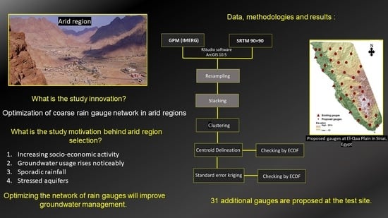
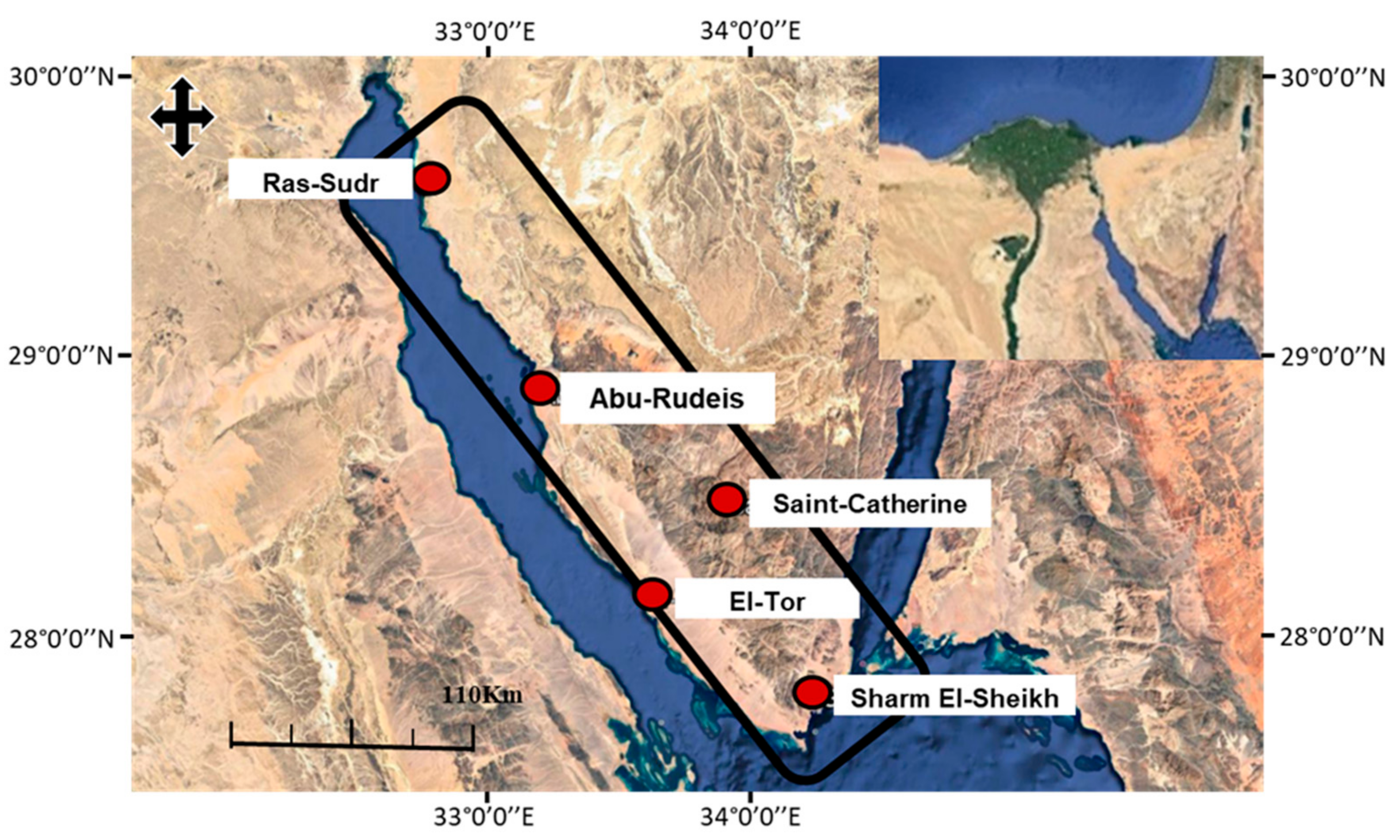
The aim of this study is to present an innovative approach for extension and optimization of rain gauge networks by using remote sensing data from satellites. The main steps engaged in this endeavor are: (i) choice of appropriate spatial remote sensing datasets to refine the given coarse gauge network; (ii) determination of appropriate mathematical methods to use in refining the network; and (iii) determination of the optimum number of gauges in topography with complex conditions. As an illustration of the proposed methodology, the El-Qaa Plain in Sinai, Egypt was chosen as the study area.

The above location was chosen because it is an arid area in the Sinai Peninsula with high potential for future development, particularly tourism. These prospects have already resulted in a steady increase in population and an extension of land utilization. As a result, local water demand is steadily rising in an area where the regional quaternary aquifer is the primary supply of groundwater [11,12]. This aquifer, which stretches from Wadi Feiran to the top of Ras-Mohamed, is mostly replenished by precipitation [13]. The region is covered by five rain gauges, which yield insufficient precipitation spatiotemporal data for groundwater management. The study area is covered by a coarse rain gauge network which makes it a very good target for testing the methodology proposed herein. Also, the study area is characterized by distinctive features such as elevation fluctuations and precipitation variability.

Two data sets were chosen in the current analysis to optimize the coarse rain gauge network. The final run of GPM (IMERG), which performed better in a previous comparative study [14], was used, along with 90 × 90 Shuttle Radar Topography Mission (SRTM) elevation data. This was achieved by the use of statistical metrics such as k-means clustering, normal error kriging, and the Empirical Cumulative Distribution Function (ECDF).

2. Materials

2.1. Study Area

The eastern side of the Gulf of Suez is one of Sinai’s most arid zones, located between latitudes 29°54′N and 27°42′N and longitudes 32°42′E and 34°06′E. The site is around 350 km long and 80 km wide [15], with altitudes above sea level, ranging from 0 to 2000 m, and strata spanning from Precambrian to Quaternary. The test site is delimited to the south by Sharm El-Sheikh, to the north by Ras-Sudr and Abu-Rudeis, and to the west and east by El-Tor and Saint Catherine, respectively (Figure 1). Any development in the research site puts significant demand on the existing aquifer, perhaps leading to a drop in the water table [16]. Precipitation is the primary recharge source for this aquifer, which spans from Wadi Feiran to Ras-head Mohamed’s [16,17,18]. The research area is equipped with only five tipping bucket rain gauges. The area covered by the test site is roughly estimated to be greater than 20,000 km².

Sherief [19] classified precipitation occurrences in the test site as light (0.1 to 1 mm), moderate (1 to 10 mm), and heavy (>10 mm). Light cases account for 61% of all annual events, 34% are moderate, and 5% are heavy. Each of these intensity levels results in a different environmental effect. On the one hand, heavy intensity events are the most severe because they cause extreme flash floods, resulting in collateral destruction and loss of life. Light intensity cases, on the other hand, aid water cycle stability at the study site through improvements in soil moisture and infiltration rates.

2.2. Integrated Multi-Satellite Retrievals for GPM (IMERG)

Over the same region, Morsy et al. [14] contrasted TRMM (Tropical Rainfall Measurement Mission) and IMERG satellite precipitation products, on the one hand, and against ground rain gauges, on the other hand. They concluded that IMERG estimations perform better than TRMM. The Spearman correlation coefficient was calculated to be 0.745 with the IMERG data, whereas much smaller values for this statistic were calculated for the TRMM data. In Figure 2, a scatterplot diagram of rain gauge measurements against the IMERG satellite retrievals is displayed. Based on those findings, the IMERG rain product was utilized in the present paper as it is more promising in the present endeavor to optimize the rain gauge network.

The state-of-the-art source of global-scale rain and snow measurements, namely, the Global Precipitation Measurement (GPM) [20,21,22]) is used in the present work. Four standard IMERG scenes have been used, each with a spatial resolution of 0.1° (or 10 × 10 km), that covered four consecutive rainy events from 2015 to 2018. The events discussed in the study occurred on 25 October 2015, 27 October 2016, 12 April 2017, and 28 April 2018; these events were classified based on Sherief’s precipitation intensity classifications (see [19]) as moderate, heavy, light, and light intensity events, respectively. These events were chosen to represent the entire spectrum of precipitation intensities in the test site. Each IMERG scene consists of a daily composite of half-hourly scenes obtained from NASA Mirador’s official website (Figure 3). The final run of the GPM (IMERG) selection criteria was presented in a companion paper [14].

2.3. Shuttle Radar Topography Mission (SRTM)

More than 80% of the world’s digital elevation models (DEMs) are provided by NASA’s Shuttle Radar Topographic Mission (SRTM). These data are freely distributed by the United States Geological Survey (USGS) and can be downloaded from the National Map Seamless Data Distribution System or the USGS FTP website. In the current study, SRTM (90 × 90 m) data were used to figure out the relationship between precipitation intensity and elevation (Figure 4). With increasing elevation, the amount of precipitation received increases [19]. Since topography influences the amount of rain collected at the test site, elevation is considered to play an important role in the present analysis.

It is worth noting here that a finer resolution for DEM has resulted in an excessive number of redundant points that overlapped throughout the ECDF curve. Implementing all of these points as potential sites for rain gauges will result in too much redundancy, unnecessary additional costs and obliterating of the aim of the research, which is the optimization of the network.

2.4. Software

To achieve the study’s goal, two software packages were used in tandem. The first is RStudio (version 1.2.1335-1) that includes three packages: the raster package, version 3.4-10, the rgdal package, version 1.5-23, and the ggplot2 package, version 3.3.3 [23,24]. The second software package is ArcGIS 10.5 that was used to process the data and complete the optimization steps.

3. Methods

To achieve the study’s aim, two mathematical approaches were integrated in a systematic way: k-means clustering and standard error kriging; k-means clustering was utilized to divide the whole range of numerical values collected by GPM and SRTM into tiny divisions of closely related values [25], and kriging of standard error was used to discover the locations with the greatest error for further optimizing the gauge placements [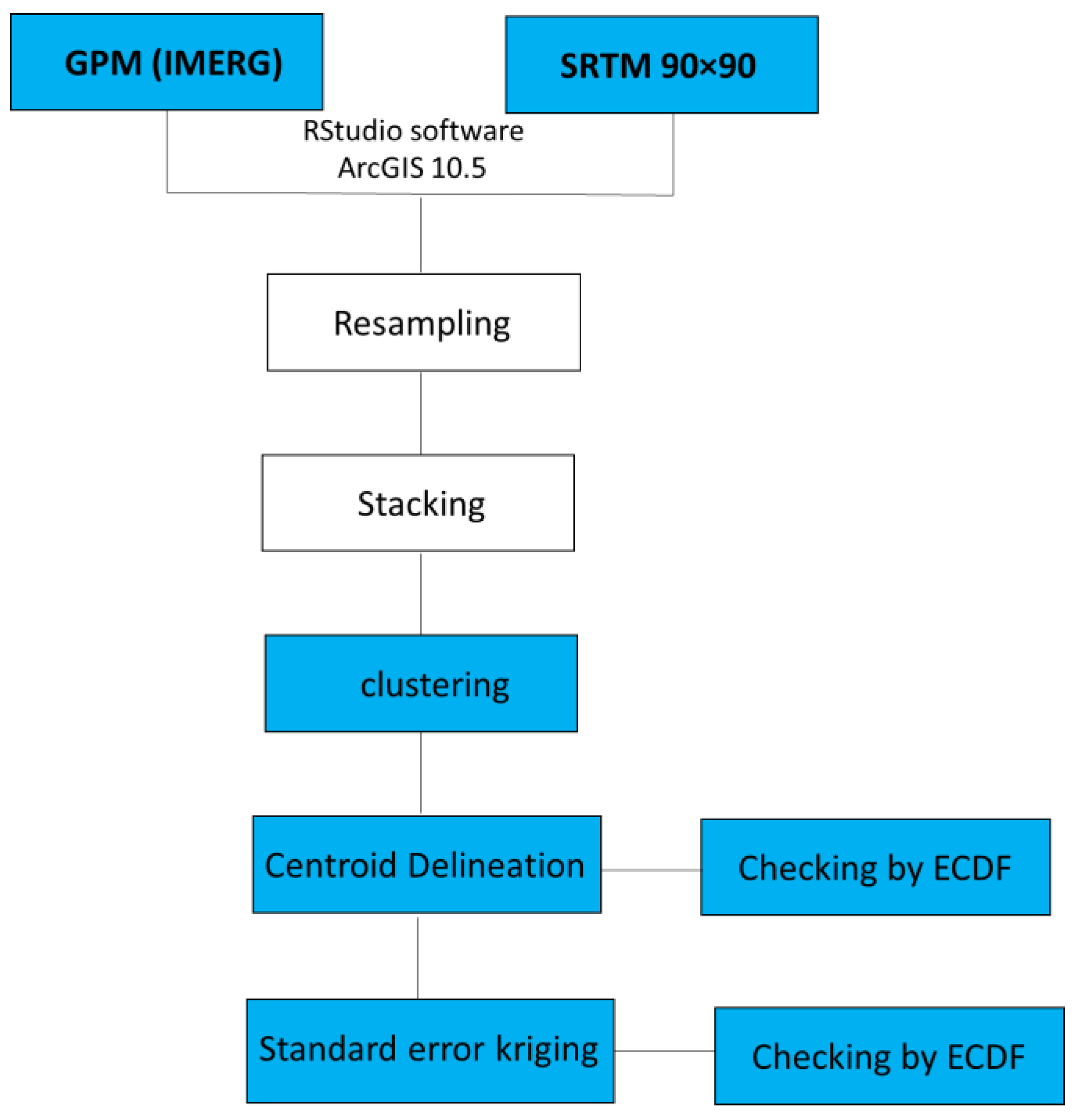11]. However, the Empirical Cumulative Distribution Function was used to identify the best position of the resultant points or gauges. The whole procedure is represented in Figure 5 and all the details of statistical metrics are given in Appendix A.

3.1. Data Resampling, Stacking and Clustering

The DEM file was resampled to match the pixel scale of the GPM (IMERG) data (10 × 10 km). The DEM file was resampled using bilinear interpolation, which is suggested for usage with continuous data, such as elevation. Furthermore, it produces clear results with a smooth appearance. The procedure was applied by using ArcGIS10.5. The coarser resolution was chosen because it would yield a smaller number of gauges to meet a minimum budget. The remote sensing-derived data scenes (GPM (IMERG) and DEM) were saved as TIFF files, stacked, and converted into point data. The stacking method is similar to producing a two-layer composite. It involves matching the pixels of the DEM file perfectly over the pixels of the GPM file in order to treat them as a single layer throughout the rest of the procedure.

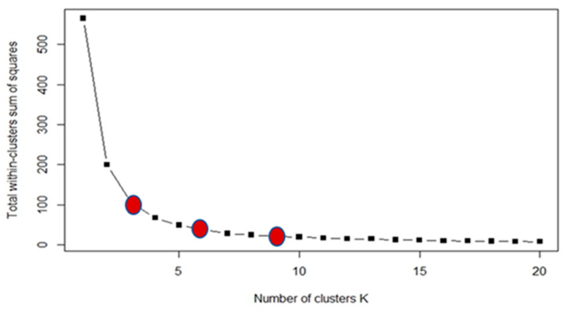
Data clustering has been described as an unsupervised machine learning technique that divides datasets into small partitions, each with nearly identical values and characteristics [12,13,26,27,28,29] but that can be distinguished from each other. The most fundamental and commonly used approach in the literature is k-means clustering. The k-means algorithm works well for numerical data that has a fixed number of clusters (k). We used the examination of an elbow graph in deciding the optimum number of clusters. The elbow graph is a visual approach in which the ‘elbow’ portion of the graph shows a wide area before plateauing [25]. Three different cluster counts were compared. Each number produced a single point file, which was subsequently converted into a raster image file, and, finally, a shapefile. The centroids for the three resulting shapefiles are computed. Specific RStudio software was used to achieve the stated goal.

3.2. The Empirical Cumulative Distribution Function

Empirical Cumulative Distribution Function is the distribution function associated with the empirical measure of a sample in statistics. It simulates empirical outcomes and compares the sample’s probability distribution to that of the population [30]. Lahiri et al. [31] developed ECDF as a random distribution function for providing a statistical description of a random field over a given area. It enables the mapping of an ordered sample of a population from minimum to maximum values and then generates a representation of how the sample is spread around the population [30].

The positions of the observed centroids (for the three chosen k-values) were tested using an ECDF. This was done to select the optimum k-value, or the number of clusters, for the test site by selecting the k-value with the best spatial coverage. This evaluation was focused on the previously mentioned raster layers.

The highest and lowest numerical limitations of the total of precipitation scenes, as well as the DEM, were recorded in greater detail to represent the population. The cluster centroids were considered as samples. The k-value that will provide the best population coverage (with its centroids) was deemed optimal and was chosen for further processing.

3.3. Minimizing Kriging Error

Using a methodology focused on reducing the Kriging error, one approach in geostatistics has been used to optimize networks by selecting the ideal number of stations and their placements [11]. This method is used to design a rain gauge network in the current investigation. In ArcGIS 10.5, the standard error kriging could be computed on a separate page. This estimates new sample locations and limits the number of samples necessary for optimal outcomes [32,33,34] by calculating the probability of a prediction being right. For the optimum sample value interpolation, this approach’s mathematical basis takes into account how much each sample should be weighted. There are fewer data points in a certain area, therefore that area has a higher level of inaccuracy, so more data points should be added there. ArcGIS 10.5 made advantage of looping to create a manageable number of steps (gauges).

The Kriging of standard error approach was used to minimize usual error observed in the previously stated 14-gauge design (nine recommended centroids + five current gauges). The nine proposed gauges represent the center of the nine computed clusters (calculated by ArcGIS10.5). In order to calculate the kriging error, we used the 14 indicated locations. The method proved effective in locating the pixel with the greatest inaccuracy when only one point was added. The entire procedure had been completed after 22 iterations.

4. Results

4.1. Data Clustering

The k-means method is better suited to numerical data with a predetermined number of clusters (k). This may be accomplished by employing the elbow technique of clustering, which is one of the oldest methods for determining the proper number of clusters for a given dataset [25]. This approach comprises a visual strategy that starts with a k-value of 2 and rises in unitary increments. The numerical scale lowers substantially at a particular value of k, forming an elbow shape followed by a plateau. The k-value is represented by the start of the plateau [25]. In the current case, the start of the plateau was hard, so one value was picked at the start of the suspicious zone, one in the center, and one at the end of the ambiguous region; then, they were all compared to get the highly advised one.

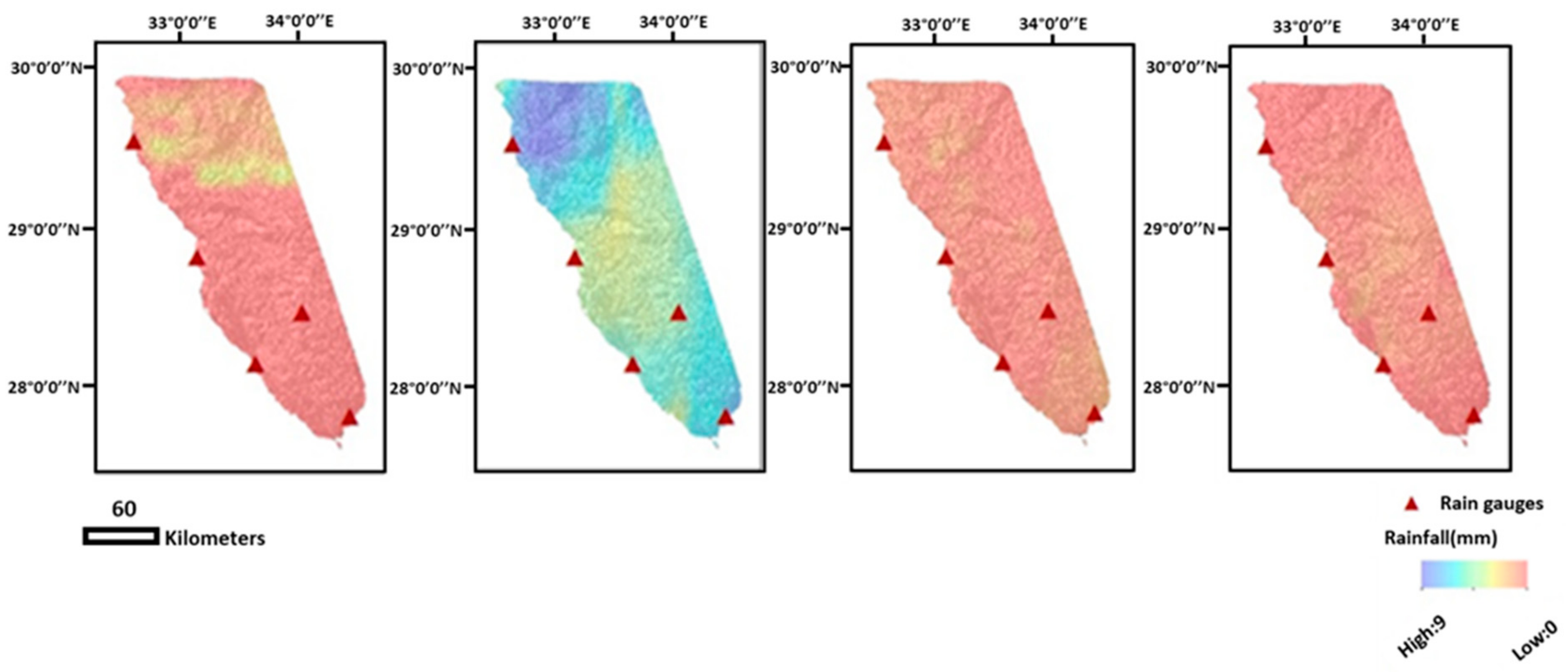
The sum of the four mentioned rainy events (four scenes) resulted in one scene with the whole range of the light, moderate, and heavy intensity events. This scene was converted to a point file. In this point file, each pixel was converted to one point, to assure that we will get the complete entire range of rainfall. The clustering procedure started with the previously mentioned point file.

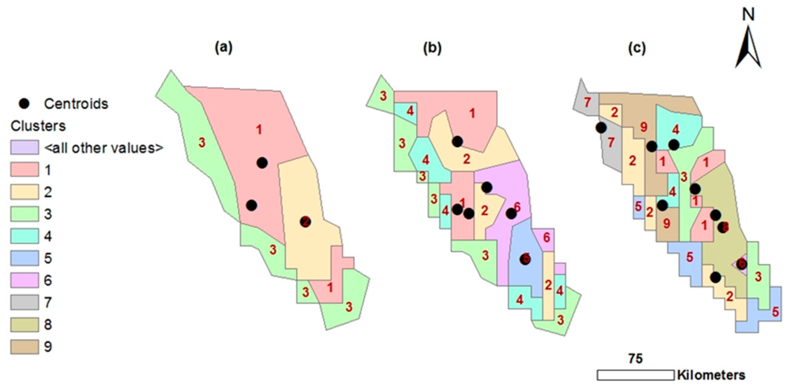
The graph produced had a large elbow-shaped area, raising questions about the optimal cluster number (Figure 6). As a result, three distinct k-values (3, 6, and 9) were visually selected and mathematically tested. Clustering the three selected values in RStudio generated three point-shape files of 3, 6, and 9 classes, which were then converted to raster files and then polygon-shape files by the ArcGIS10.5 software (Figure 7). Each type register resulted in three, six, and nine centroids. Since each resulting cluster was formed of several partitions reflecting the same numerical limitations in the polygon shape files (Figure 7), all the individual partitions of a cluster were merged to determine the position of the centroid automatically at its virtual center (ArcGIS 10.5).

4.2. Checking by ECDF

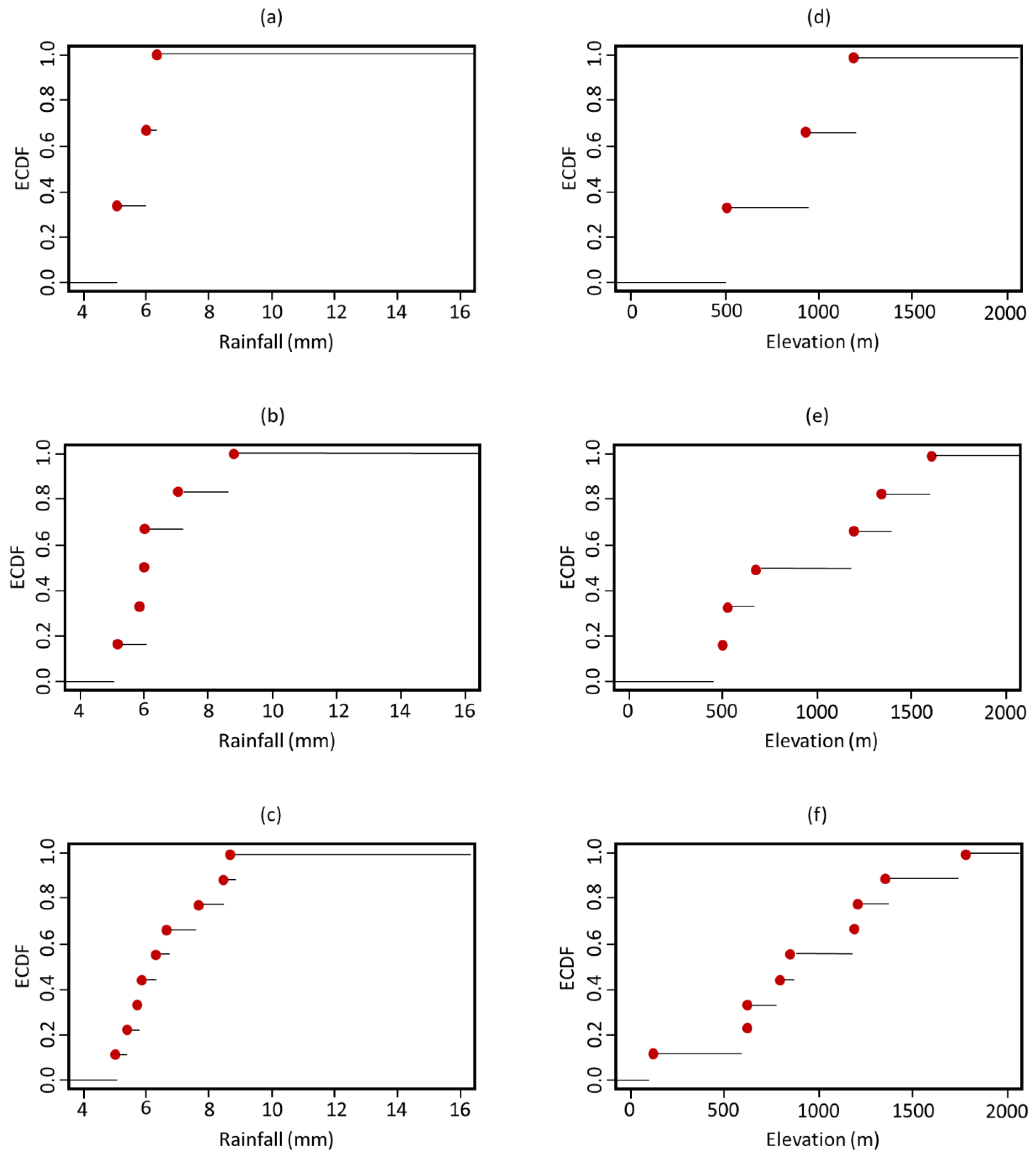
ECDF was applied to the previously listed three, six, and nine cluster centroids to assess the optimum k-value as well as to calculate the spatial coverage of the proposed centroids over the precipitation and elevation ranges. This necessitated the feedback of upper and lower limits for precipitation (4–16 mm) and elevation (0–2000 m), all of which were used to determine the x-axis scales in Figure 8. The sample size of the three centroids covered a very limited part of the population, precipitation intensity less than 7 mm, and elevation less than 1200 m. A notable empty space was noted between the 7 and 16 mm values in the precipitation graphs, as well as the 0 to 500 m, 500 to 1000 m, and 1200 to 2000 m elevations in the associated elevation graphs. The sample size of the six centroids covered a very limited part of the precipitation population and a relatively wider part of the elevation population, less than 9 mm and 1700 m. The six-centroid distribution’s ECDF revealed a gap between the 7 and 9 mm values, as well as the 9 and 16 mm values. The elevation curve also showed a gap between 0 and 500 m and 600 and 1400 m. The sample size of the nine centroids covered a very limited part of the precipitation intensity population, less than 9 mm, and almost the whole elevation population with some gaps. The ECDF of the nine-centroid distribution showed less vacant ranges, which was present this time in the precipitation range of 9 to 16 mm and in the elevation curves of 100 to 600 m and 1300 to 1700 m.

Although all of the above findings showed differences in the centroids’ distribution, the nine-centroid distribution had the best coverage, as compared to the three- and six-centroid distributions. As a result, the nine centroids (plus the five current gauges making a total of 14 sites) were used as the basis for a subsequent process to improve their coverage and performance.

The coverage limits of each cluster are reported in order to determine the cause for inadequate coverage despite the optimal cluster number (

Table 1. Lower and upper limits of each cluster as determined by using the complete range of precipitation values (4–16 mm).

Cluster No.	Precipitation Min. (mm)	Precipitation Max. (mm)
1	5	11.5
2	3	13.3
3	5	9.7
4	3.7	10.3
5	5	13.6
6	5.2	7.7
7	5	14
8	4.8	10.3
9	3.7	12.7

and

Table 2. Lower and upper limits of each cluster as determined by using the complete range of elevation values (0–2000 m).

Cluster No.	Elevation Min. (m)	Elevation Max. (m)
1	721	1115
2	262	404
3	448	860
4	522	691
5	6	103
6	1609	2000
7	124	369
8	1172	1524
9	436	556

). The lower and upper limits of each resultant cluster are covering a very wide range of precipitation compared to the used range (4 to 16 mm). As a result, one centroid of each cluster was insufficient to reflect the entire cluster values. Compared to the wide spectra of elevation (0 to 2000 m), each related cluster covered a limited range of elevations and one centroid in each cluster reflected the value range.

Because of the wider range of elevation, as compared to precipitation, the software allowed the elevation values to mask the precipitation values during the clustering process. This is the reason why the coverage of the elevation spectra with the nine centroids appears to be more promising (Figure 8c,f).

4.3. Kriging of Standard Error

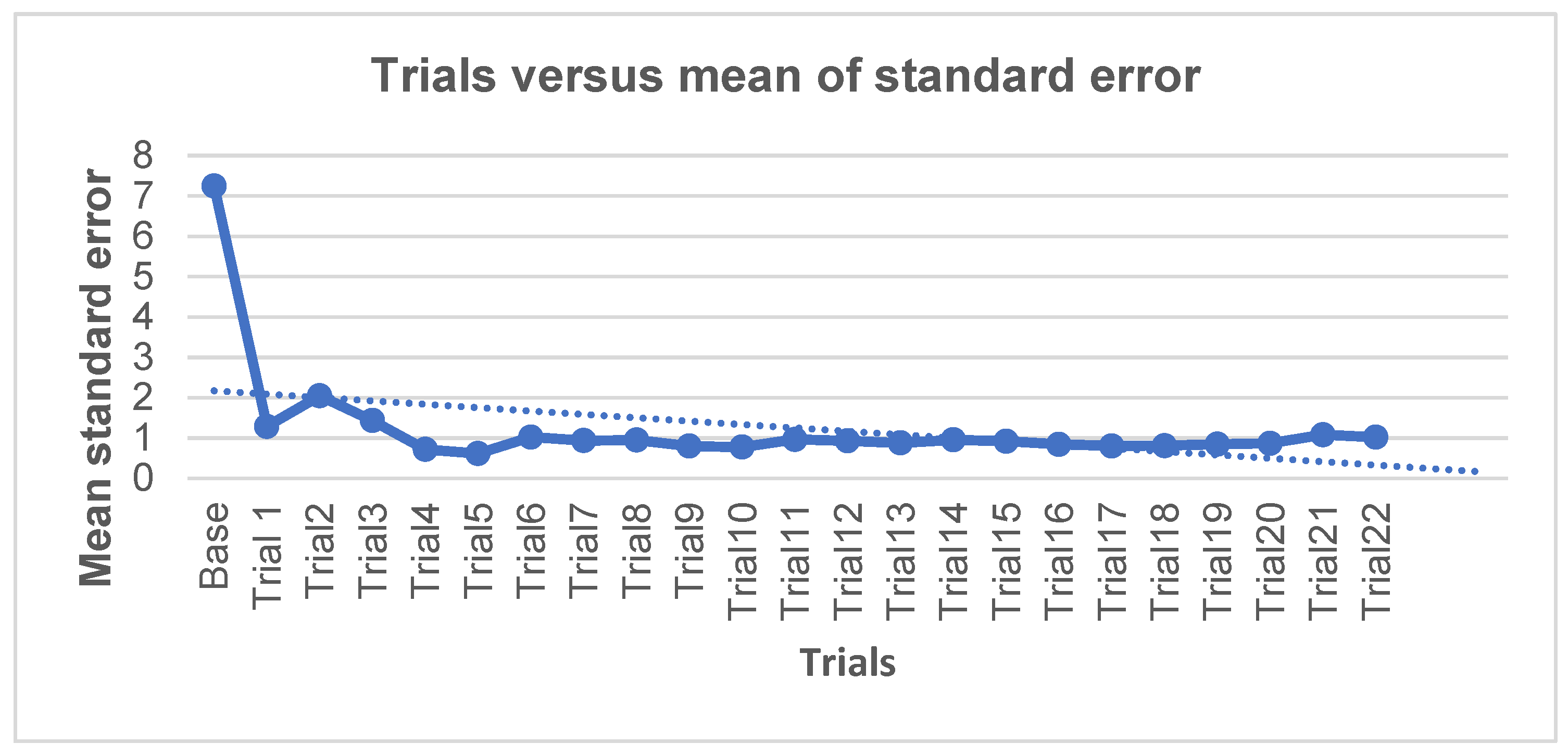
The Kriging of standard error technique was also used to eradicate the typical error observed in the previously described 14-gauge design (nine proposed centroids plus five existing gauges). This entailed applying a single gauge at a time for a total of 22 iterations (Figure 9). The inclusion of the first argument reduced the mean standard error from 7.2 to 1.2 mm. As the standard error rose from 1.2 to 2.0 by the third point, the resulting graph formed a plateau. Following that, it fell to 0.7 by the fifth trial, followed by a minor depression under the sixth and seventh trials (values of 0.6 and 1.0, respectively).

A plateau was achieved during the eighth and ninth trials, with only minor negative variations in the tenth, eleventh, and twelfth trials (0.79, 0.77, and 0.96, respectively). This plateau was maintained for the 13th, 14th, and 15th trials, with a marginal decline evident for the 16th to 19th trials (0.92, 0.84, 0.80, 0.80, and 0.4, respectively). The curve started to climb marginally again by the 20th experiment, with values of 0.84, 0.86, and 1.08 for the 20th, 21st, and 22nd iterations, respectively. The final trial yielded a result of 1.02.

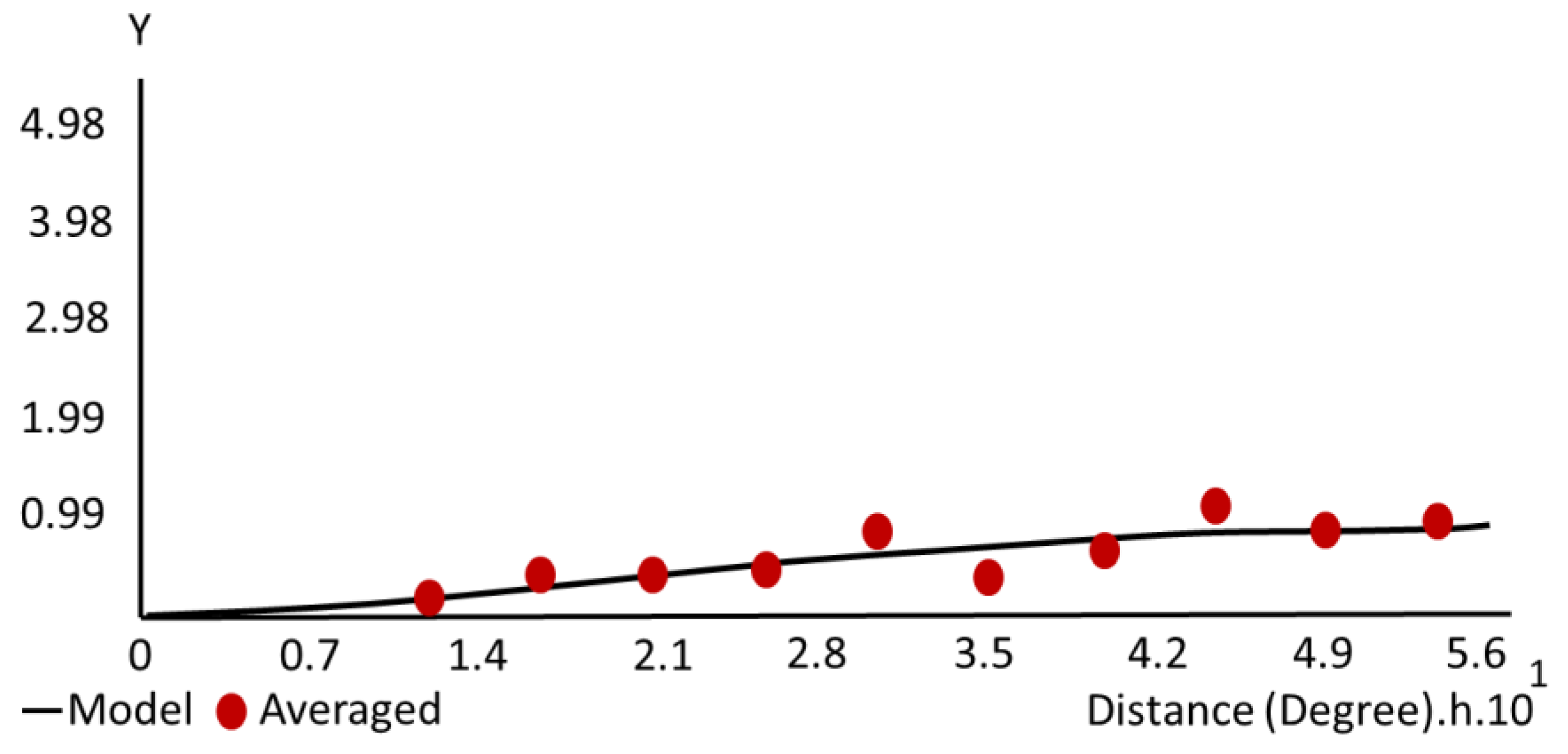
Tobler’s First Law of Geography was used to measure the resulting Gaussian variograms. According to this rule, everything is connected to everything else, but closer things are more related than distant things [35]. The developed variograms showed distance in degrees on the x-axis and variance between variables on the y-axis. As can be shown, by the 22nd trial, as the difference between two points (h) increased, so did the variance (y). Furthermore, 22 of the graphs had binned points scattered across the model, suggesting high variance. Nineteen graphs demonstrated positive autocorrelation, while four did not (non-rising model) (Figure 10). Variograms showed varying nugget, sill, and range values (

Table 3. Nugget, sill, and range values as recorded by each variogram over the 22 trials.

Trials	Nugget	Sill	Major Range
Base	0.46	0.32	2.47
Trial 1	0.48	0.33	0.52
Trial 2	0.008	0.81	0.47
Trial 3	0.008	0.73	0.40
Trial 4	0.007	0.81	0.40
Trial 5	0.00	0.77	0.37
Trial 6	0.06	0.65	0.37
Trial 7	0.24	0.31	0.37
Trial 8	0.61	0.28	1.02
Trial 9	0.70	0.36	1.13
Trial 10	0.00	0.61	0.57
Trial 11	0.00	0.65	0.57
Trial 12	0.37	0.12	0.37
Trial 13	0.08	0.54	0.37
Trial 14	0.00	0.74	0.37
Trial 15	0.62	0.48	0.53
Trial 16	0.71	0.61	0.54
Trial 17	0.88	0.88	0.69
Trial 18	0.95	0.95	0.69
Trial 19	0.91	0.86	0.55
Trial 20	0.63	0.25	0.74
Trial 21	0.35	0.41	0.64
Trial 22	0.00	0.97	0.56

). However, binned points were fitted around the model in the final experiment, meaning that the least difference (between adjacent and distant points) could be found here. Trial 22 generated a random field with a sill of 0.97 and a major range of 0.56, due to the absence of a nugget effect at the origin and the maximum sill value. Given these measurements, Trial 22 was deemed optimal, and no further iterations were carried out. The highest results at the lowest expense have been identified.

4.4. Double-Checking with ECDF

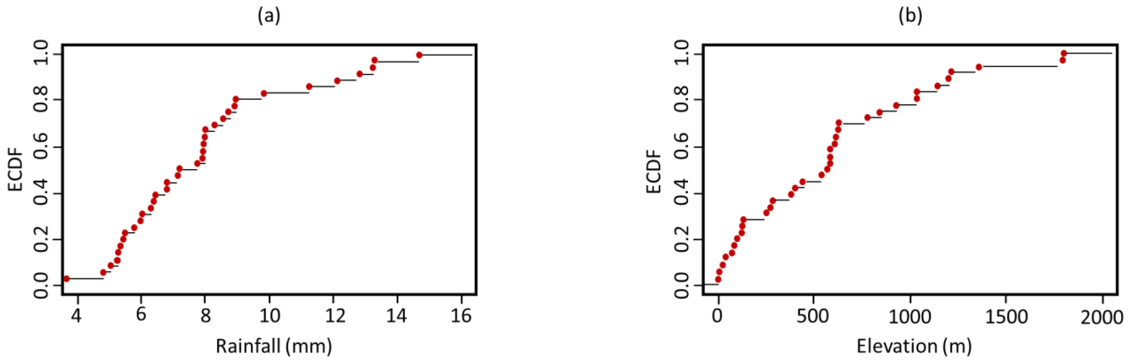
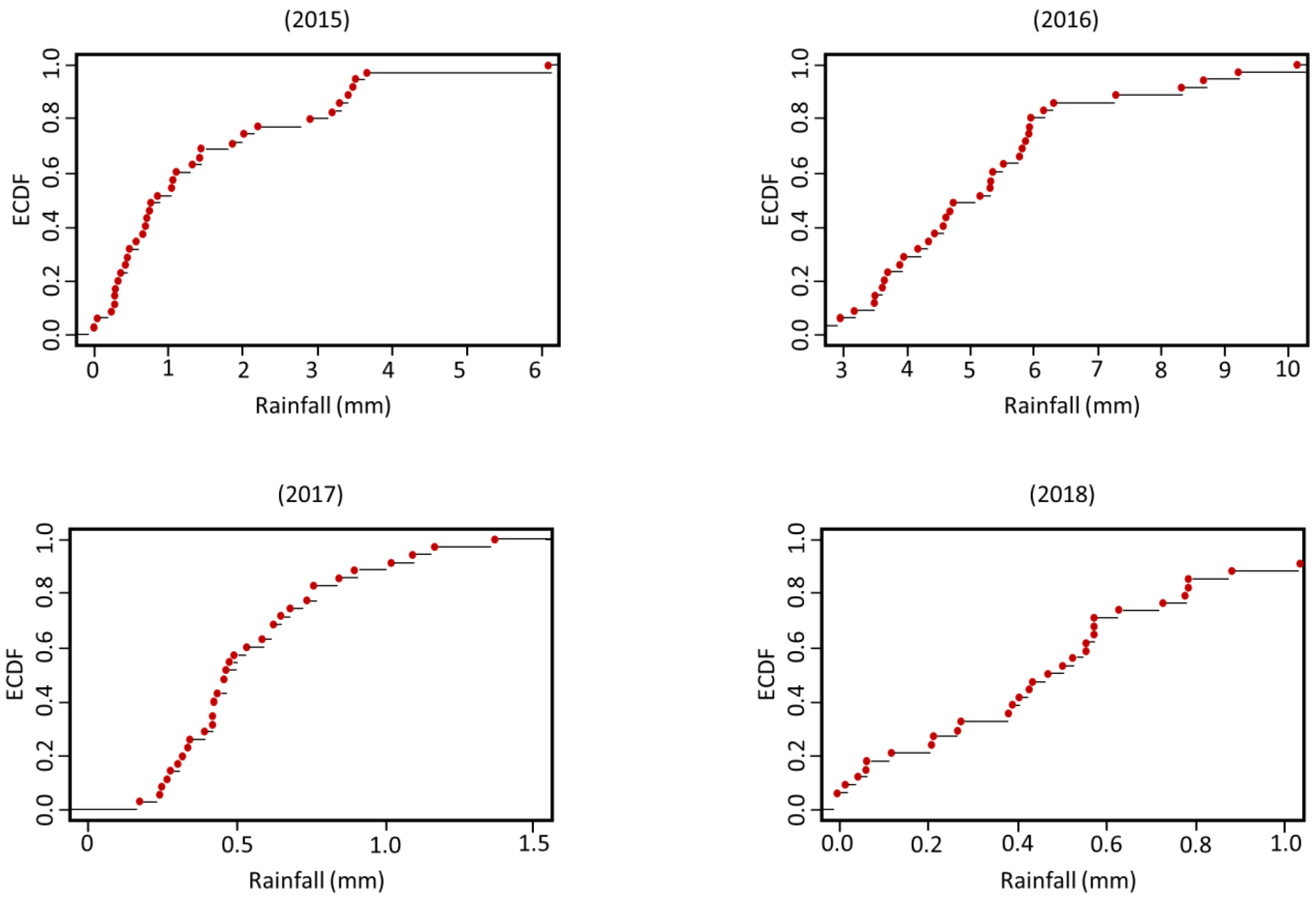
The ECDF was used once more to assess the combined positions of the current and planned rain gauges, 36 in total. The findings of an ECDF test on the level of precipitation spectrum coverage offered by the entire planned gauge network are shown in Figure 11a, with very positive results supporting the position selection technique. Figure 11b depicts the effects of a test on the level of coverage by elevation, with the graph displaying positive results once again, except for a minor empty region between 1350 and 1650 m. Gauge coverage was checked for each precipitation occurrence to further validate the techniques. Complete coverage was noted with the events in 2016, 2017, and 2018 (Figure 12). For the 2015 event, however, there was a gap between 3.8 and 6 mm.

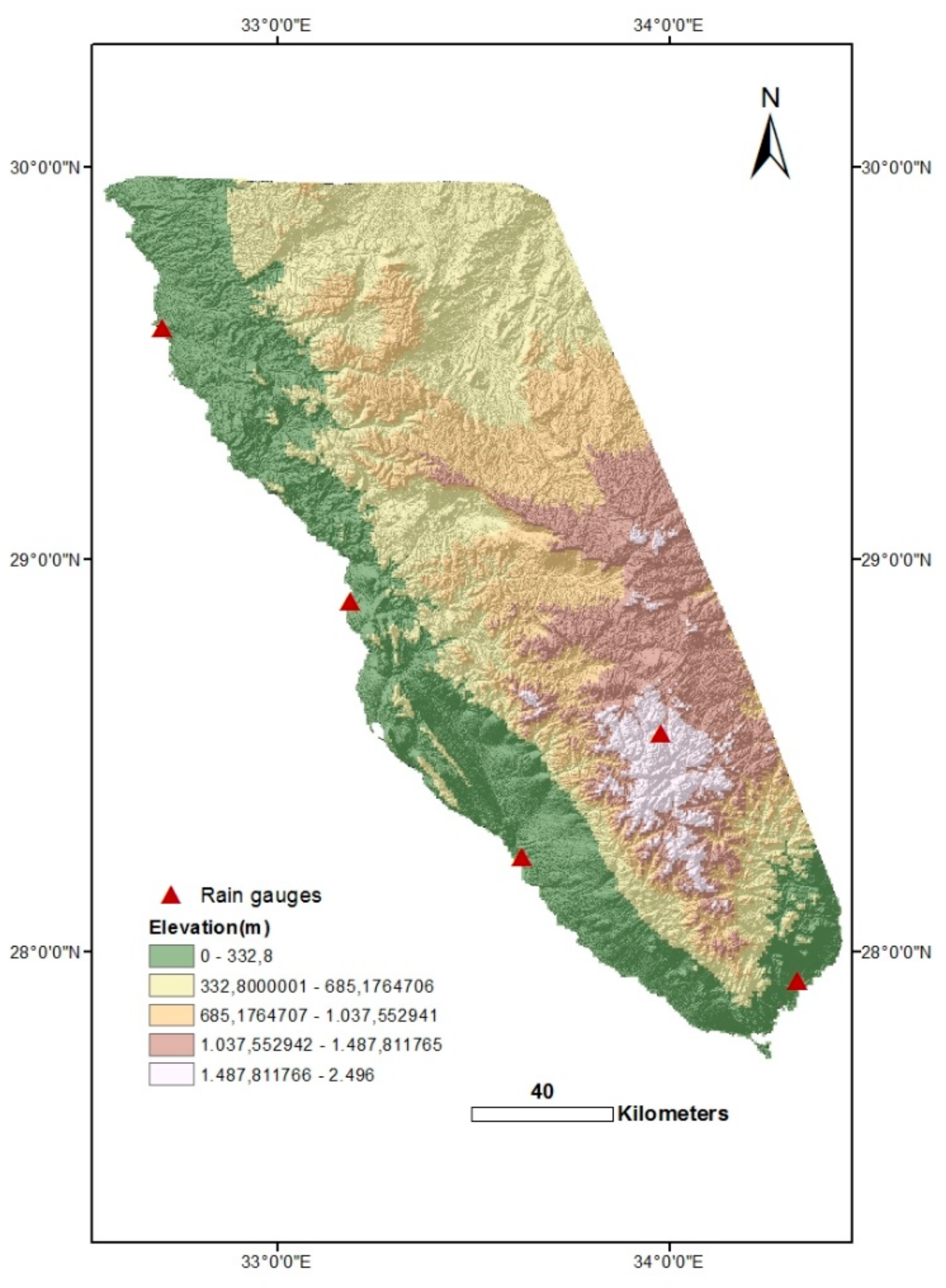
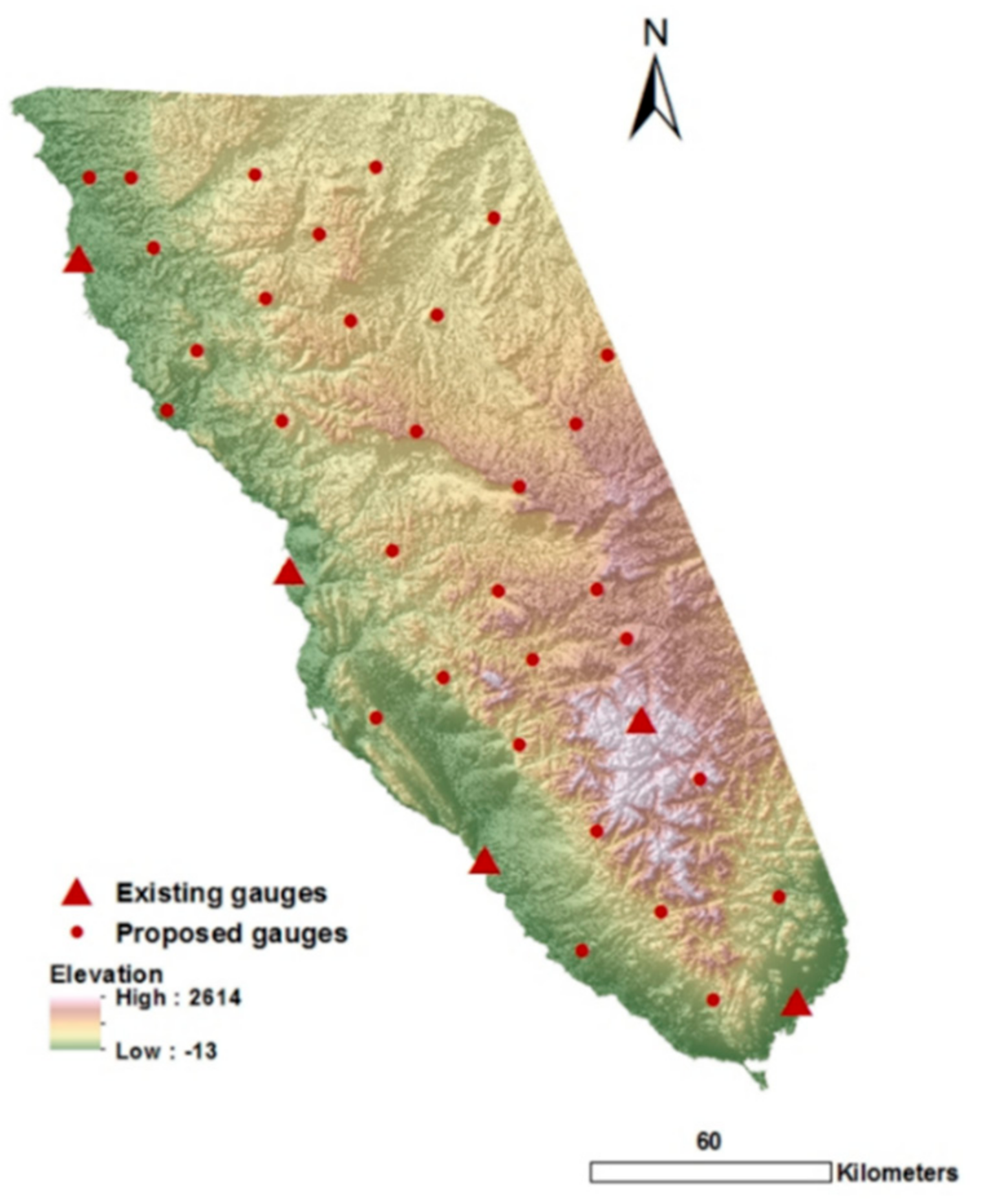
Overall, the approach produced satisfactory positive findings that will provide the investigated region with an optimized rain gauge coverage on a limited budget. Therefore, the locations of the proposed gauges (produced by clustering and kriging error) and the existing gauges were plotted together on the elevation map (Figure 13).

5. Discussion

As the spatiotemporal resolution of satellite-based rainfall datasets increases, an increasing interest in the utilization of such datasets is noted in precipitation-related scientific research with orientation in hydrological applications. Although the use of satellite-based rainfall datasets has several indispensable advantages, they have to be exploited within the framework of the known limitations and their suitability for a particular application and must be scrutinized first. For example, the effectiveness of remote sensing techniques in estimating light precipitation or snow must be taken into account in any such endeavor [36,37]. Li et al. [38] have examined the suitability of IMERG data over China and noted a mismatch between these data and ground-based measurements under light precipitation conditions. Also, Skofronick-Jackson et al. [39] stressed the need for investigators using spaceborne techniques to carefully consider the algorithms adopted when analyzing surface snow retrievals from satellites.

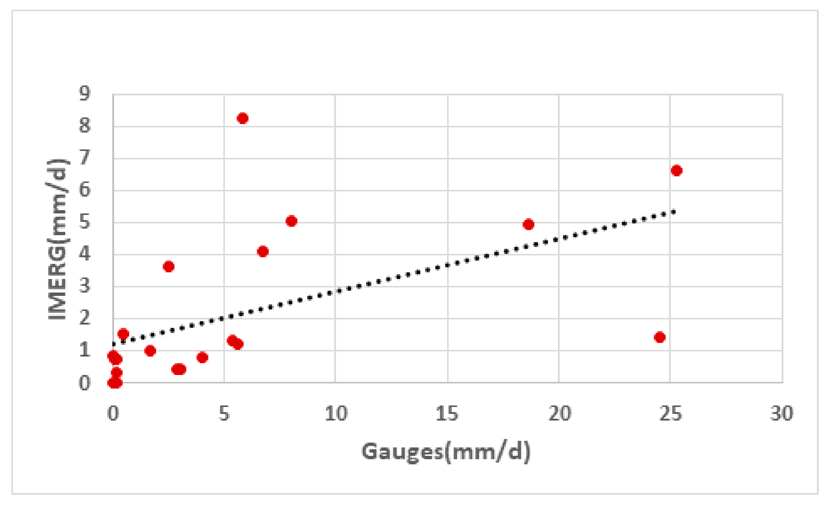
Bearing in mind the above, the suitability of IMERG precipitation datasets was investigated over El-Qaa Plain in the preceding research [14] where the frequency of light events is high. The results of that study were encouraging, as IMERG datasets from the light-intensity events were highly correlated with the in-situ measurements.

The present research comprises an extension of a previously published companion paper (see [14]) which concerns arid regions with a coarse ground rain gauge network, resulting in large uncertainties in the establishment of the spatiotemporal distribution of precipitation, leading to hampered knowledge in the water cycle equilibrium. Under these insufficient ground data coverage conditions, satellite remote sensing data can provide an alternative, although their validation with in-situ data encompasses still a source of uncertainty. Optimizing the rain gauge network for the region under study was considered as the best solution, both for improving the knowledge of the local hydrological conditions but also for validating any available precipitation data base, including satellite remote sensing sources.

The technique for coarse network optimization differs significantly from that for fine network optimization [40,41]. As a result, the current research proposed an optimized approach that relies heavily on remote sensing data to determine the best number and positions for the proposed gauges. The first part of the analysis validated the performance of IMERG at the test site. Four scenes spanning the years 2015 to 2018 were combined with SRTM 3 (90 × 90 m) to determine the positions of the new gauges. In an attempt to reduce the required budget, a coarse resolution of 10 × 10 km was selected to reduce the number of clusters and the resulting proposed gauges. Furthermore, the severity of the precipitation did not differ significantly at the study site, with the greatest difference occurring between the plain and hill regions.

To establish new rain gauge sites, two main techniques were used. The first included k-means clustering, which was initially thought to be adequate for the current analysis. However, the number of locations generated was inadequate to accommodate the entire range of precipitation and elevation values. As a result, a second method, namely, the kriging of standard error, was used, with the gauges calculated by k-means clustering serving as a basis. The kriging of normal error was looped through 22 iterations, resulting in the finding of new positions for 22 gauges. ECDF then reviewed the 31 gauges that resulted, in addition to the five existing gauges, and the findings revealed an outstanding coverage over the full spectrum of total precipitation, elevation, and for each individual precipitation occurrence (from the years 2016, 2017, and 2018). However, there were just a few open spots for the 2015 event. These data were accurate enough to be used at the test site. Considering that the potential position confirmation can be accomplished by k-means clustering, in terms of upkeep, the planned gauges farthest from actual settlements and roads could be omitted, but this could affect the coverage quality of the proposed rain gauge network.

In general, humid regions have a sufficient network of gauges and they do not have a water scarcity problem, and of course different water management approaches are adopted. The site in the present research is a dry region that has undergone a rapid increase in socioeconomic activity. These activities result in more intensive ground water use, which is depleted at a fast rate; therefore, it is critical to understand the entire water cycle balance in such locations in order to properly manage the current groundwater water sources. Knowledge of the rainfall spatiotemporal distribution is crucial as rainfall is a primary factor influencing the water cycle’s balance in the area. However, there are not enough gauges to accurately assess the spatiotemporal distribution of rainfall. As a result, installing additional rain gauges in dry places is the only way to improve ground water management. In these communities, managing ground water resources means ensuring the continuity of life, development, and economic activities. If subsequent readings from an upgraded rain gauge network reveal that the amount of rainfall is insufficient to replenish the aquifers and sustain life in the study region, then other alternative solutions should be sought (e.g., the building of dams, flowing water harvesting, etc).

Uncertainty in the distribution of meteorological variables over mountainous regions is a factor that must be contemplated in the choice of appropriate sites for the installation of instruments for their measurement. In particular, as exemplified by Gultepe et al. [42], the variability of precipitation over complex terrains is usually quite large, as precipitation amounts may increase or decrease with elevation, depending on the distribution of thermodynamical conditions, as well as on a number of other factors. In the same research, Gultepe et al. [42] show how interactions with other meteorological variables can affect precipitation measured on the ground. In general, a straightforward definition of even the main factors driving the observed variability is not an easy task, as many underlying mechanisms could be responsible for this behavior. Such factors can become more pronounced over complex terrain; in essence, any factor that can modify the direction and intensity of the airflow during a storm could in turn modify the spatial distribution of precipitation in the region and thus the relationship between precipitation and elevation. Variability over a complex terrain is difficult to understand with a small number of stations, especially over an arid environment. Nevertheless, variability is not easier to explain even with a denser rain gauge network, bearing in mind the diversity of the sources of such variability. Dynamic factors have been identified to have a major impact on precipitation variability (see [43]) but other factors have also been examined. To name only few of the attempts to explain the variability of precipitation over complex terrain, one example is the recent study over the Alpine region in which a very large number of rain gauges over the area had been exploited in an attempt to quantify the sources of anthropogenic effects on mountain precipitation [44], by combining data from many stations into classes of homogeneous station elevation and compared the precipitation among different classes. Also, it is worth mentioning the study by Givati and Rosenfeld [45] who provide evidence that air-pollution aerosols can suppress precipitation in orographic cloud.

In the present study, despite the limited number of cases studied, it is clear that, for all precipitation intensities that were considered, the more elevated rain gauges (e.g., Saint-Catherine station) recorded the highest rainfall. This is also demonstrated in the data collected by Sherief [19] for the same research site.

6. Conclusions

The current research introduces a new integrated methodology for targeting the upgrading and improvement of coarse rain gauge networks in arid regions and a number of reasons were cited above for choosing a dry location to test the suggested procedure’s implementation. The findings of the present research support the impression that remote sensing data is an excellent option for places with no or few rain gauges, as it enables the gathering of more frequent records at a higher resolution. However, it is common that satellite-based estimates demonstrate uncertainty and underestimate rainfall records in highly elevated locations. This is why the authors combined GPM (IMERG) rainfall retrievals with elevation data to obtain the optimum outcome. The proposed procedure in the current research is applicable to dry areas which suffer from lack of in-situ precipitation data and for which the competent authorities wish to make plans for an expansion of their rain gauge networks. The suggested procedure’s correctness may be proved soon after these additional rain gauges are installed, and more data is gathered.

There are many constraints that may influence the implementation of the proposed gauges network, such as proximity to an internet connection or power supply. Many of the suggested gauges are located a long distance away from such utilities. However, there are many options that may be contemplated, such as the use of solar energy as an alternative source of power. The option of using local individuals to obtain the precipitation readings during rainy events and report them accordingly using available telecommunication facilities might also be another alternative to lacking internet connection. Indeed, an investigation that was carried out following the results of this study has revealed that many of the suggested gauges are easily accessible through the local road network (although few of the proposed locations are isolated, being at a distance from roads and towns, but they are reachable). It is recommended that all the proposed gauges be installed in order to ensure optimal coverage for both precipitation and elevation.

One of the scopes of future expansion of the research by using the approach described in the paper is to test the proposed methodology in areas with a denser network. However, if the network is already dense, then there might be no real need to add more stations but maybe the need would be to propose a more representative distribution of the rain gauges by repositioning them; to this end, the same technique can be employed.