Abstract
Near surface wind speed has significant impacts on ecological environment change and climate change. Based on the CN05.1 observation data (a gridded monthly dataset with the resolution of 0.25 latitude by 0.25 longitude over China), this study evaluated the ability of 25 Global Climate Models (GCMs) from Coupled Model Intercomparison Project phase 6 (CMIP6) in simulating the wind speed in the Arid Region of Northwest China (ARNC) during 1971–2014. Then, the temporal and spatial variations in the surface wind speed of ARNC in the 21st century were projected under four Shared Socioeconomic Pathways (SSPs), SSP1-2.6, SSP2-4.5, SSP3-7.0, and SP5-8.5. The results reveal that the preferred-model ensemble (PME) can fairly evaluate the temporal and spatial distribution of surface wind speed with the temporal and spatial correlation coefficients exceeding 0.5 at the significance level of p = 0.05 when compared to the 25 single models and their ensemble mean. After deviation correction, the PME can reproduce the distribution characteristics of high wind speed in the east and low in the west, high in mountainous areas, and low in basins. Unfortunately, no models or model ensemble can accurately reproduce the decreasing magnitude of observed wind speed. In the 21st century, the surface wind speed in the ARNC is projected to increase under SSP1-2.6 scenario but will decrease remarkably under the other three scenarios. Moreover, the higher the emission scenarios, the more significant the surface wind speed decreases. Spatially, the wind speed will increase significantly in the west and southeast of Xinjiang, decrease in the north of Xinjiang and the south of Tarim Basin. What’s more, under the four scenarios, the surface wind speed will decrease in spring, summer and autumn, especially in summer, and increase in winter. The wind speed will decrease significantly in the north of Tianshan Mountains in summer, decrease significantly in the north of Xinjiang and the southern edge of Tarim Basin in spring and autumn, and increase in fluctuation with high values in Tianshan Mountains in winter.
1. Introduction
As an influencing factor of ecological environment change and climate change, surface wind speed has a significant impact on the wind energy industry, surface evapotranspiration, hydrological cycle and wind-related natural disasters (such as sandstorm, tornados, and typhoons) [1,2,3,4,5]. Thus, it is crucial to study the variations of surface wind speed, especially in the areas rich in wind energy resources, such as China. In the context of global warming, many studies have pointed out that the global surface wind speed has decreased over the past half-century (termed “global stilling”) [6]. Tian et al. [7] studied the variation of surface wind speed in the northern hemisphere through the observation data from 1979 to 2016 and concluded that in most areas of the northern hemisphere, including North America, Europe, and Asia, the surface wind speed had shown a downward trend in the past 40 years, such as Portugal, Canada, South Korea, the United States, France, and China [8,9,10,11,12,13]. In general, the above studies have made a detailed and in-depth analysis of the temporal and spatial changes of wind speed over the past half-century, and revealed the seasonal variation of wind speed, but pay less attention to future projection.
The ARNC, our study area, is located in the hinterland of the Eurasian continent. With complex terrain, sensitive response to climate system change, and frequent sand and dust events, it is one of the areas richest in wind energy resources in China and has excellent potential for wind energy development. It has become one of the hotspot areas of wind resources research [14,15]. Many studies show that [16,17,18], over the past half-century, the change of surface wind speed in the ARNC is consistent with that of the whole of China and even the northern hemisphere, showing a decreasing trend with a larger magnitude than the whole China. The complexity of the terrain in the ARNC determines the regional differences in the temporal and spatial distribution of surface wind energy resources. Therefore, an in-depth study is necessary to investigate the temporal-spatial distribution and variation of surface wind speed in the ARNC and the projection of future wind speed, which can provide a scientific basis for the development of wind energy resources and the site selection of wind farms, which is of great significance to the utilization and planning of future wind energy in China.
The GCM (Global Climate Model, see Table 1 for Nomenclature, similarly hereinafter) is the major tool for simulating and projecting climate change. Using GCM to study future climate change can effectively deal with the risks of ecological environment protection and social development brought by climate change. The Coupled Model Intercomparison Project (CMIP), initiated and organized by the World Climate Research Programme’s (WCRP) Working Group on Coupled Modelling (WGCM) in 1995 [19]. Its initial purpose was to compare the performance of a limited number of global coupled climate models at that time. In addition, an important feature is that the GCM output participating in CMIP is made public in a standard format through the Earth System Grid Federation (ESGF) data replication Center for analysis by the wider climate community and users [20]. Its research results are a significant part of the Intergovernmental Panel on Climate Change (IPCC) assessment of future climate change.

Table 1.
Important nomenclature.
The CMIP6 is currently in phase 6, which has evolved over several phases such as CMIP1, CMIP2, CMIP3 and CMIP5 [21,22]. Compared with the previous stages, the process involved in the models consideration of CMIP6 is more complex, and the resolution of atmospheric and ocean models is significantly improved [23]. Compared with CMIP5 models, the most significant feature of CMIP6 is the combination of radiation forcing levels of the Representative Concentration Pathways (RCPs) in CMIP5 and the Shared Socioeconomic Pathways (SSPs), and three new emission paths (SSP1-1.9, SSP3-7.0 and SSP4-3.4) are added to fill the gap between the typical paths of CMIP5 [24]. Based on the Shared Socioeconomic Pathways (SSPs) and anthropogenic emission trends, CMIP6 put forward new future scenarios, including seven scenarios (SSP1-1.9, SSP1-2.6, SSP2-4.5, SSP3-7.0, SSP4-3.4, SSP4-6.0 and SSP5-8.5) with each SSP representing a development model [25]. Driven by IPCC, a lot of achievements in climate change simulation and prediction by CMIP model data have been made, especially in simulating and predicting temperature and precipitation [26,27,28].
Currently, there have been relatively few studies on the future change of surface wind speed or wind energy resources, partly due to the poor performance of reanalysis datasets in wind speed and the scarcity of high-quality observation datasets. The existing studies are mainly concentrated in some European and American countries. Pryor et al. used the statistical downscaling method to predict wind speed and found that there was no significant change in wind speed in northern Europe in the middle and late 21st century [29]. Carvalho et al. analyzed the impact of climate change on large-scale wind energy resources in Europe in the future by CMIP5 [30]. Li et al. obtained the distribution characteristics of future wind energy changes in China using the statistical downscaling method [31]. Jiang et al. estimated the changes of China’s surface wind speed in the 21st century under three human emission scenarios, high emission (A2), medium emission (A1B), and low emission (B1) [32]. The above studies are all large and medium-sized, ignoring the impact of local climate characteristics on wind speed. At the same time, due to the limitations of the model itself, there is uncertainty in the analysis of regional wind speed change. Relevant studies show that [33,34,35], CMIP5 and CMIP6 models have achieved good performance in wind speed simulation and prediction, but there are still apparent deviations, although it is a macro-scale study like China. Therefore, it is necessary and vital to correct the deviation to reduce the uncertainty. However, the deviation correction work has seldom been done in the previous wind speed research in the ARNC, which was further studied in this study.
Fully considering the contributions and shortcomings of the above research, this study focuses on the regional scale (mesoscale) and evaluates the simulation ability of the newly released 25 CMIP6 GCMs (Table 2) and two model ensembles based on the observation data. A better model suitable for wind speed simulation in the ARNC is selected, providing a specific reference for similar regional studies. At the same time, we corrected the deviation of the model data to improve the research accuracy and then selected the deviation-corrected PME to predict the temporal and spatial changes of wind speed under four SSP scenarios. The study provides a scientific basis for the rational development and utilization of wind energy resources in the ARNC.
Table 2.
Information of CMIP6 models used in this study and the correlation between model data and observation data.
The main aims of this study include: (i) evaluation of simulation ability of CMIP6 model data; (ii) comparison of the spatiotemporal characteristics of mean wind speed between PME and revised PME; (iii) future projections of mean wind speed under four emission scenarios based on deviation-corrected PME.
2. Materials and Methods
2.1. Materials
Model data. The monthly surface 10m mean wind speed data of 25 GCMs outputs (from https://esgf-node.llnl.gov/search/cmip6/, accessed on 20 June 2021) was provided by the CMIP6 of the WCRP (Table 2). To ensure the integrity of data and the consistency of results, the GCMs used in this work are the monthly data under the “r1i1p1f1” operation results, which means the first realization (r1), first initialization (i1), first physics (p1) and first forcing (f1) (https://github.com/WCRP-CMIP/CMIP6CVs/, accessed on 20 May 2021). In order to compare with observations, the 25 model data with different spatial resolutions were interpolated to the same resolution of 0.25° × 0.25°. The historical simulation data from 1971 to 2014 and the future projection data from 2015 to 2100 were used for analysis. Four scenarios (Table 3), SSP1-2.6, SSP2-4.5, SSP3-7.0, and SSP5-8.5, were chosen to represent sustainability, middle of the road, regional rivalry, and fossil-fueled development pathway, respectively [20]. Five periods, 1995–2014, 2021–2040, 2041–2060, 2061–2080, and 2081–2100 were divided, representing the baseline period (BP), near future (NF), mid future (MF), far future (FF), and final period (FP), respectively.
Table 3.
The Shared Socioeconomic Pathways (SSP) of CMIP6 used in this study.
Observation data. The CN05.1 gridded monthly observation dataset from 1971 to 2014 was used for assessing the simulation ability of CMIP6 model data. The dataset was developed by Wu et al. based on the observation data from more than 2400 meteorological stations in China, using the thin plate spline method, with a resolution of 0.25° × 0.25° [36]. In terms of seasonal division, March to May is spring, June to August summer, September to November autumn, and December to next February winter.
2.2. Methods
2.2.1. Model Evaluation
The standardized spatial Taylor map was used to quantitatively evaluate the spatial distribution capacity of CMIP6 models. That is, the three indicators of correlation coefficient (r), Root-Mean-Square Difference (RMSD), and standard deviation ratio (S) were computed to evaluate models and the Taylor map was used for concise statistics [37]. The closer to the observations, the stronger the simulation ability of the model is.
The standard deviation ratio () is the ratio of standard deviation of simulation field to standard deviation of observation field. The closer the data between the simulation field and the observation field is, the closer S is to 1, and the better the model simulation ability is.
2.2.2. Deviation Correction
Firstly, a univariate linear regression model between the observed data and the average of the multi-model historical simulation set is established:
where was the total number of the samples, and were the return factors, and was the return residual.
Then, according to the return factors, the above formula was applied to the average of the sets of multiple patterns in the future, and the correct value of the estimated data was:
3. Results
3.1. Evaluation of Simulation Ability of CMIP6 Model Data
3.1.1. Temporal Simulation Ability
In terms of the correlation coefficient of each model from 1971 to 2014 (Table 2), there are five models (ACCESS-ESM1-5, BCC-CSM2-MR, EC-Earth3, EC-Earth3-Veg-LR, and NorESM2-LM) exceed 0.3 (p < 0.05). For the MRI-ESM2-0 model, although the time correlation coefficient is only 0.24, which is second to the above five models, the spatial correlation coefficient is 0.48 (p < 0.01), indicating that its comprehensive simulation ability is strong. Therefore, the above six models are selected as the preferred models and formed the PME. All the models involved are called multi-model ensemble (MME). From the correlation coefficient alone, PME (r = 0.62, p < 0.01) is closer than MME (r = 0.43, p < 0.01) to the observed data.
The variation in observed and simulated surface wind speed during 1971–2014 (Figure 1a) shows that fifteen models (such as ACCESS-CM2, ACCESS-ESM1-5, AWI-CM-1-1-MR, CESM2-WACCM and EC-Earth3, etc.) and two ensembles are closer to the observations, with the wind speed ranging from 2.7 m/s to 4.2 m/s. Three models (BCC-CSM2-MR, FGOALS-f3-L, MRI-ESM2-0) overestimate wind speed and their average wind speeds were 5.0 m/s, 5.1 m/s, and 6.1 m/s respectively, which was significantly higher than the observed wind speed (3.2 m/s). Seven models (CAS-ESM2-0, CMCC-CM2-SR5, CMCC-CM2-SR5, etc.) underestimate wind speed, and the variation range of wind speed with time is between 1.7 m/s and 2.5 m/s. In terms of the long-term trends (Figure 1b), only eight single models (ACCESS-ESM1-5, BCC-CSM2-MR, EC-Earth3, etc.) and two ensembles (PME and MME) to capture the downward trend of surface wind speed in the ARNC during 1972-2014 with the significance test of 10%. Among these models, the largest is BCC-CSM2-MR (−0.0264 m/s/10a), but its downward rate is far lower than the observed data (−0.168 m/s/10a). The mean wind speed simulated by other modes has no obvious downward trend (−0.005~0.0096 m/s/10a) or upward trend (0.0002~0.0118 m/s/10a). That is, none of the models can reproduce the same trend as the observation value as the magnitude.
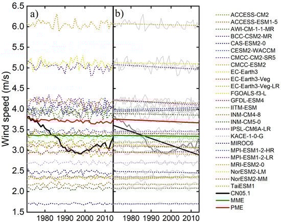
Figure 1.
Variations (a) and trends (b) of observed (black solid line) and simulated (color dot line, red and green solid line) surface wind speed in the ARNC from 1971 to 2014.
3.1.2. Spatial Simulation Ability
In order to better evaluate the spatial simulation ability of CMIP6 models on surface wind speed in the ARNC and evaluate the simulation performance of different models, the spatial correlation coefficient, RMSD, and standard deviation of multi-year surface wind speed are calculated and expressed in the form of Taylor chart (Figure 2). The star in the figure represents the observation results, and the upper and lower case letters represent the evaluation results of the corresponding model. It can be seen from the figure that the spatial correlation coefficient between most models (13) and observation data is more prominent than 0.4, and the RMSD is less than 1, indicating that most models can simulate the spatial distribution of multi-year average annual wind speed. The correlation coefficients of MME and PME exceed 0.5, and the RMSD is within 1, but the standard deviation ratio of PME is closer to 1, so PME has a better ability to simulate spatial distribution. Comprehensively considering the time and space simulation ability, PME is more stable in simulation performance, which is better than single models and MME. Therefore, PME is selected to analyze the future surface wind speed change in the study.
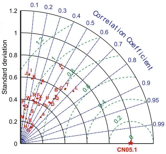
Figure 2.
Taylor chart of CMIP6 models in simulating wind speed in the ARNC during 1971–2014.
3.2. Deviation Correction of CMIP6 Model Data
Although PME performs well in all single models and model ensembles, it still overestimates the wind speed (Figure 3), and there is a noticeable deviation in the spatial distribution. Compared with the spatial distribution of the observation data in the same period (Figure 3c), the model data (Figure 3d) can simulate the characteristics of large wind speed in the east and south of the ARNC and small in the west, but cannot simulate the characteristics of large wind speed in mountains and small in basins. Therefore, it is necessary to correct the PME data further.
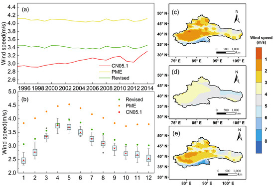
Figure 3.
Comparison between revised/unrevised PME and observation in time and space. (a) annual mean surface wind speed (b) monthly mean surface wind speed (c) observed wind speed (d) simulated wind speed by the unrevised PME (e) simulated wind speed by the revised PME.
The method of the univariate linear regression model is used to correct the deviation of PME data. Firstly, a univariate linear regression model between PME and the observation data from 1961 to 1994 is established, and the obtained linear relationship is used to verify the monthly scale model data from 1995 to 2014. It can be seen from Figure 3 that the model data after deviation correction has been significantly improved in time and space. The corrected surface wind speed (3.41 m/s) is closer to the observed (3.06 m/s) than that before correction (4.08 m/s), and the monthly surface wind speed is also more consistent with the observation. From the spatial distribution of observed wind speed (Figure 3c), the annual wind speed in the ARNC is mainly high in western Inner Mongolia and Hexi Corridor, low in Southern Xinjiang, high in the mountainous area, and low in the basin. Compared to uncorrected data (Figure 3d), the corrected PME (Figure 3e) reproduces the spatial distribution pattern of mean wind speed. Therefore, the above correction method is used to correct the deviation of PME data under four scenarios in the future 2015–2100.
3.3. Projection of Annual Wind Speed in the ARNC
3.3.1. Temporal Trend
Figure 4 displays the prediction results of PME after deviation correction on the surface wind speed trends in the 21st century under different emission scenarios. The results show that the mean wind speed is increasing under SSP1-2.6 and decreasing under SSP2-4.5, SSP3-7.0, and SSP5-8.5, with a downward rate of −0.0007~−0.0072 m/s/10a, and the annual wind speed changes more significantly under SSP3-7.0 and SSP5-8.5, which is consistent with the study by Krishnan et al. [38].
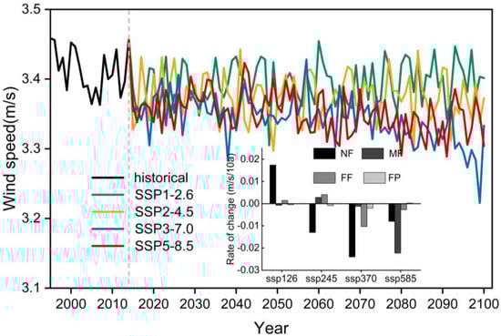
Figure 4.
Variations in projected annual wind speed in the ARNC from 1995 to 2100 under different emission scenarios. The black bar chart shows the variation trend of surface wind speed in NF, MF, FF and FP.
In terms of the time period, under SSP1-2.6 and SSP2-4.5, the surface wind speed in the 21st century shows a fluctuating change, and the trend is the most significant in NF, which are 0.0174 m/s/10a, and −0.013 m/s/10a, respectively. Under the scenario of SSP3-7.0, the surface wind speed in the 21st century continuous to decline, NF decreases the fastest (−0.024 m/s/10a) and MF decreases the slowest (−0.0013 m/s/10a). Under the SSP5-8.5 scenario, the surface wind speed in the 21st century first decreases and then increases, with NF, MF, and FF all showing a downward trend. The decline rate of MF is the fastest (−0.0223 m/s/10a) and FP a slight upward trend (0.0003 m/s/10a).
Overall, the difference of surface wind speed trend under the four emission scenarios is mild in NF and MF, and it tends to be significant after MF. Among them, the wind speed decline rate is the fastest under SSP3-7.0, small under SSP2-4.5 and SSP5-8.5, while the wind speed still shows a weak upward trend under SSP1-2.6.
3.3.2. Spatial Variation
From the spatial difference distribution of NF, MF, FF, and FP relative to BP under the four emission scenarios of SSP1-2.6, SSP2-4.5, SSP3-7.0, and SSP5-8.5 (Figure 5), the surface wind speed in the ARNC will mainly decrease compared with BP as a whole in the future, and there is an upward trend in some areas. The higher the emission scenario is, the greater the wind speed decreases.
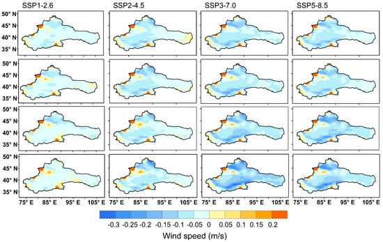
Figure 5.
Spatial difference distribution of NF (row 1), MF (row 2), FF (row 3), and FP (row 4) relative to BP (1995–2014) under four emission scenarios.
Specifically, under SSP1-2.6, compared with BP, the regions with increased wind speed in the 21st century are mainly observed over the Tianshan Mountains and Eastern Kunlun Mountains, and the regions with wind speed decrease less than −0.05 m/s are mainly observed over the Northern Xinjiang. As time goes on, the regions with increased wind speed gradually increase, and those with wind speed decrease less than −0.05 m/s decrease. Under the scenarios of SSP2-4.5, SSP3-7.0, and SSP5-8.5, the high-value area (>0.15 m/s) with increased surface wind speed in the ARNC appears in the western edge and southeast of Xinjiang. The high-value area with decreased surface wind speed (<−0.15 m/s) is distributed in the north of Tianshan Mountain and the south of Tarim Basin, which is more significant in FF and FP.
3.4. Projection of Seasonal Wind Speed in the ARNC
3.4.1. Temporal Trend
Seasonal differences in wind speed exist (Figure 6). Generally speaking, the surface wind speed increases in winter and decreases in spring, summer and autumn, with the most apparent decline in summer. SSP5-8.5 scenario has the fastest decline of surface wind speed in spring, with a decline rate of −0.0094 m/s/10a. The most significant decrease of surface wind speed in summer and autumn is SSP3-7.0, and the decline rates are −0.0132 m/s/10a and −0.0135 m/s/10a, respectively. The maximum increase of surface wind speed in winter is SSP5-8.5, up to 0.0083 m/s/10a.
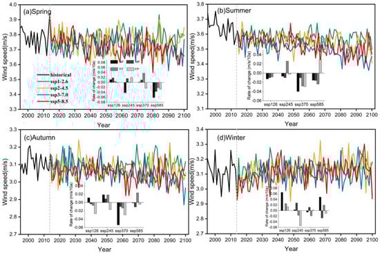
Figure 6.
Variations in the seasonal wind speed in the ARNC from 1995 to 2100 under four emission scenarios. The black bar chart shows the variation trend of surface wind speed in NF, MF, FF and FP.
In terms of periods, the seasonal surface wind speed in the ARNC changes slightly differently in the four periods of the 21st century under the four scenarios. In NF, the surface wind speed decreases obviously in spring, summer and autumn, and increases in winter. In MF, the change of surface wind speed in four seasons is not obvious under each scenario, and the change range is concentrated between −0.02~0.02 m/s/10a. In FF, the surface wind speed is projected to increase significantly in spring and autumn but decrease significantly in summer and autumn. In FP, the wind speed in four seasons is projected to decrease significantly.
3.4.2. Spatial Variation
Figure 7 shows the spatial distribution of seasonal mean wind speed relative to BP in NF, MF, FF, and FP under four emission scenarios. The results show that in spring, under SSP1-2.6 and SSP2-4.5, the mean wind speed is projected to increase in the central, south of Xinjiang and Inner Mongolia, decrease in Northern Xinjiang, with the overall variation ranging −0.1~0.1 m/s and some areas more than 0.1 m/s. Under SSP3-7.0 and SSP5-8.5, the spatial distribution of surface wind speed changes similarly in the four periods; that is, there is a significant decline (<−0.1 m/s) in a large area of Northern Xinjiang and Southeastern Tarim Basin. In summer, the change in the spatial distribution of wind speed under four SSP scenarios is relatively consistent. The whole study area generally shows a downward trend with high values in the north of Xinjiang, while an increase in some areas on the edge of the west and south of Xinjiang.
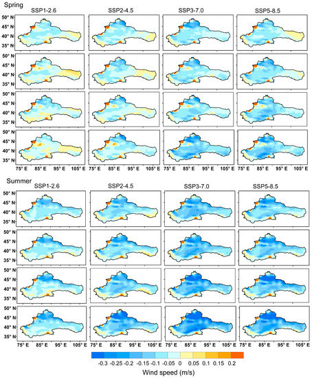
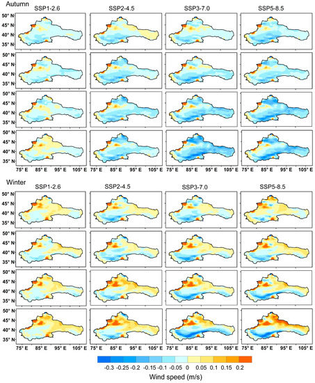
Figure 7.
Spatial difference distribution of seasonal mean wind speed relative to BP in NF (row 1), MF (row 2), FF (row 3), and FP (row 4) under four emission scenarios.
The spatial variation of wind speed in autumn is similar to that in spring. Under the SSP1-2.6 scenario, the area where the wind speed increases are mainly in the middle of Xinjiang and extend to the whole of northern Xinjiang at the end of the period. Under SSP2-4.5, SSP3-7.0, and SSP5-8.5, the wind speed increases in the Tianshan Mountains and decreases in the north and southeast of Xinjiang and Inner Mongolia. The change of wind speed in winter is opposite to that in summer. The wind speed increases obviously under each scenario, and the high-value area is mainly in Tianshan Mountains in Northern Xinjiang. By the end of the 21st century, the high-value area extends to large areas north to 40° N in the study area.
Generally speaking, the surface wind speed in spring, summer, and autumn in the 21st century mainly decreases in different scenarios and periods and increases in some parts of the Tianshan Mountains. In winter, the whole study area has a significant upward wind speed, and the decreasing area is only in Southern Xinjiang and Hexi Corridor. As time goes by, the higher the emission scenario, the more significant the trend of surface wind speed decreasing (or increasing).
4. Discussion
GCM is an essential means to estimate future wind energy resources, which have higher reliability for projecting future trends and large-scale average conditions. However, the regional wind speed is not only affected by the atmospheric circulation, but also the local climate characteristics, especially in the ARNC, where the natural environment is complex and the terrain fluctuates greatly. Therefore, there is still great uncertainty in a single climate model simulation of surface wind speed in the ARNC. In this study, the simulation performance of multi-model ensemble tends to be more stable and closer to the observations with a higher simulation accuracy than the single climate model. Therefore, adopting the multi-model ensemble is one way to increase model simulation reliability [39,40].
The current research results show that the surface wind speed in China and even the world will still decrease in the 21st century under the background of continuous global warming, and the decline of annual mean wind speed in our study area is very similar to that in China [34,35,41]. The difference is that China′s mean wind speed is projected to increase in summer (the largest trend 0.004 m/s/10a) and decrease in winter (the largest trend −0.012 m/s/10a) during 2015–2100 under various scenarios, and the magnitude of decrease in winter is more significant than that in annual (the largest trend −0.008 m/s/10a) [34]. While in this study, the surface wind speed in the ARNC in the 21st century is decreasing in summer (the largest trend −0.0132 m/s/10a) and increasing in winter (the largest trend 0.0083 m/s/10a).
The possible reason is that the decreasing surface wind speed in China is related to the weakening trend of the monsoon in East Asia and South Asia [42,43]. Besides, some related studies [44,45,46] predict that the Asian summer monsoon index will increase significantly, and the winter monsoon index will weaken significantly in the future. However, the ARNC is deeply inland and weakly affected by the monsoon, so the variation trends of the surface wind speed in summer and winter are different from those in China. Such a similar situation also occurred in India [47], in the summer of the 21st century, the surface wind speed will increase by 1~15% on both the eastern coast (Eastern Ghats) and the western coast (Western Ghats) of India, while in the Indo-Gangetic Basin, Gangetic West Bengal, and adjoining Bangladesh wind shows a decreasing trend by 1~5%. The decrease of wind speed is attributed to the decrease of atmospheric instability, such as convective activity related to surface wind speed and the increase of potential temperature. The cause of wind speed reduction is complex. In addition to monsoon factors, it is also affected by many factors such as dust storms, cold waves, extratropical cyclone reduction, and underlying surface anomaly. In-depth research is needed to reveal the interaction and feedback mechanism and quantitatively evaluate the contribution of each factor.
Although the climate models participating in CMIP6 have higher simulation accuracy than CMIP5, the horizontal resolution is still more than 100 km, suitable for large-scale research. When simulating in the ARNC, there is still a specific deviation in the long-term change in historical surface wind speed when simulated by each single model or model mean. After deviation correction, the model can greatly improve the simulation accuracy and reduce the uncertainty of simulation results. Therefore, more attention should be paid to the comparison and application of various deviation correction methods in regional research in subsequent research. At the same time, the use of high-resolution Regional Climate Models (RCMs) and downscaling methods are still of great significance in the study of regional scale simulation and prediction, which is also a problem that needs to be solved in the field of current and future climate change [48,49]. This will play an important role in promoting future research on the change of regional wind energy resources and their climate impact, the exploitable amount of wind energy resources, strong winds and, other extreme weather and climate events.
5. Conclusions
This study evaluated the performance of 25 CMIP6 models and 2 model ensembles (MME and PME) in simulating the surface wind speed in the ARNC based on the CN05.1 observation data. Then we used the PME with better simulation ability to project the change in wind speed under the four SSP scenarios after deviation correction. The research conclusions are as follows.
(1) PME outperforms the 25 single model and MME in simulating the temporal and spatial distribution of surface wind speed. The temporal and spatial correlation coefficients of PME are 0.62 and 0.5, respectively, which is more stable and reliable in the simulation and projection.
(2) The surface wind speed (3.41 m/s) by the deviation-corrected PME is closer to the observation (3.06 m/s), and the monthly change is also consistent with the observed data. Spatially, the PME can better reproduce the spatial distribution characteristics of the mean wind speed in the ARNC; that is, the wind speed is high in Inner Mongolia and Hexi Corridor and low in Southern Xinjiang and high in mountainous areas, and low in basins.
(3) Under the four SSP scenarios, the emission scenarios except for SSP1-2.6 show a decreasing trend in wind speed, while SSP1-2.6 shows a slightly increasing trend. The higher the radiation force is, the more significant the annual mean wind speed decreases. The difference in wind speed under each scenario tends to be significant after the middle period of the 21st century (MF). Spatially, the significant increase (>0.15 m/s) of wind speed appears in the western edge and southeast of Xinjiang, and the significant decrease (<−0.15 m/s) shows in the north of Xinjiang and the south of Tarim Basin.
(4) Under the four scenarios, the surface wind speed in the ARNC is projected to decline in spring, summer, and autumn, and the most apparent decreasing trend occurs in summer. While in winter, it increases in apparent fluctuations. Spatially, the wind speed decreases significantly over Northern Xinjiang and the southern edge of Tarim Basin in spring and autumn, with the most significant decline in the north of the Tianshan Mountains. The wind speed in winter increases significantly in Tianshan Mountains.
Author Contributions
Conceptualization, C.X.; Data curation, C.X. and Y.L. (Yunxia Long); Formal analysis, Y.L. (Yunxia Long); Methodology, Y.L. (Yunxia Long), F.L. and G.Y.; Software, Y.L. (Yongchang Liu); Writing—original draft, Y.L. (Yunxia Long) All authors have read and agreed to the published version of the manuscript.
Funding
This work was supported by the National Natural Science Foundation of China (42067062). The funder is Changchun Xu and the funding number is 42067062.
Institutional Review Board Statement
Not applicable.
Informed Consent Statement
Not applicable.
Data Availability Statement
The CN05.1 data obtained from Wu et al. The CMIP6 model data come from https://esgf-node.llnl.gov/search/cmip6/, accessed on 20 June 2021.
Conflicts of Interest
The authors declare no conflict of interest.
References
- Chen, B.Q.; Yun, T.; An, F.; Kou, W.L.; Li, H.L.; Luo, H.X.; Yang, C.; Wang, Q.F.; Sun, R.; Wu, Z.X. Assessment of tornado disaster in rubber plantation in western Hainan using and sat and sentinel-2 time series images. Natl. Remote Sens. Bull. 2021, 25, 816–829. [Google Scholar]
- Wang, C.Z.; Niu, S.J.; Wang, L.N. Multi-timescale Variation of Sand-dust Storm in China during 1958–2007. Trans. Atmos. Sci. 2009, 32, 507–512. [Google Scholar]
- Donohue, R.J.; McVicar, T.; Roderick, M. Assessing the ability of potential evaporation formulations to capture the dynamics in evaporative demand within a changing climate. J. Hydrol. 2010, 386, 186–197. [Google Scholar] [CrossRef]
- McMahon, T.A.; Peel, M.C.; Lowe, L.; Srikanthan, R.; McVicar, T.R. Estimating actual, potential, reference crop and pan evaporation using standard meteorological data: A pragmatic synthesis. Hydrol. Earth Syst. Sci. 2013, 17, 1331–1363. [Google Scholar] [CrossRef]
- Zeng, Z.; Ziegler, A.D.; Searchinger, T.; Yang, L.; Chen, A.; Ju, K.; Piao, S.; Li, L.Z.X.; Ciais, P.; Chen, D.; et al. A reversal in global terrestrial stilling and its implications for wind energy production. Nat. Clim. Chang. 2019, 9, 979–985. [Google Scholar] [CrossRef]
- Roderick, M.; Rotstayn, L.; Farquhar, G.; Hobbins, M. On the attribution of changing pan evaporation. Geophys. Res. Lett. 2007, 34, L17403. [Google Scholar] [CrossRef]
- Tian, Q.; Huang, G.; Hu, K.; Niyogi, D. Observed and global climate model based changes in wind power potential over the Northern Hemisphere during 1979–2016. Energy 2019, 167, 1224–1235. [Google Scholar] [CrossRef]
- Homogenization and Assessment of Observed Near-Surface Wind Speed Trends over Spain and Portugal, 1961–2011. J. Clim. 2014, 27, 3692–3712. [CrossRef]
- Kim, J.; Paik, K. Recent recovery of surface wind speed after decadal decrease: A focus on South Korea. Clim. Dyn. 2015, 45, 1699–1712. [Google Scholar] [CrossRef]
- Malloy, J.W.; Krahenbuhl, D.S.; Bush, C.E.; Balling, R.C.; Santoro, M.M.; White, J.R.; Elder, R.C.; Pace, M.B.; Cerveny, R.S. A Surface Wind Extremes (“Wind Lulls” and “Wind Blows”) Climatology for Central North America and Adjoining Oceans (1979–2012). J. Appl. Meteorol. Clim. 2015, 54, 643–657. [Google Scholar] [CrossRef][Green Version]
- Najac, J.; Lac, C.; Terray, L. Impact of climate change on surface winds in France using a statistical-dynamical downscaling method with mesoscale modelling. Int. J. Clim. 2011, 31, 415–430. [Google Scholar] [CrossRef]
- Tuller, S.E. Measured wind speed trends on the west coast of Canada. Int. J. Clim. 2004, 24, 1359–1374. [Google Scholar] [CrossRef]
- Feng, Y.; Que, L.; Feng, J. Spatiotemporal characteristics of wind energy resources from 1960 to 2016 over China. Atmos. Ocean. Sci. Lett. 2019, 13, 136–145. [Google Scholar] [CrossRef]
- Ding, C.X.; Yan, J.P.; Li, M.M. Climate Change and Response characteristics to Wind Speed in Northwestern China. Bull. Soil Water Conserv. 2014, 34, 134–137. [Google Scholar] [CrossRef]
- Xia, Y.F.; Zhang, X.W. China distributed wind power white paper. Wind. Energy 2018, 07, 28–31. [Google Scholar]
- Huang, X.Y.; Zhang, M.J.; Wang, S.J.; Xin, H.; He, J.Y. Variation characteristics of sunshine hours and wind speed in Northwest China in recent 50 years. J. Nat. Resour. 2011, 26, 825–835. [Google Scholar]
- Lu, J.Y.; Yan, J.P.; Wang, P.T.; Liu, Y.L. Wind Speed Change Characteristics of Shaanxi-gansu-ningxia Area in 1960–2014. J. Desert Res. 2017, 37, 554–561. [Google Scholar]
- Wang, N.; You, Q.L.; Liu, J.J. The long-term trend of surface wind speed in China from 1979 to 2014. J. Nat. Resour. 2019, 34, 1531–1542. [Google Scholar]
- Meehl, G.A.; Boer, G.J.; Covey, C.; Latif, M.; Stouffer, R.J. Intercomparison makes for a better climate model. Eos Trans. Am. Geophys. Union 1997, 78, 445–451. [Google Scholar] [CrossRef]
- Eyring, V.; Bony, S.; Meehl, G.A.; Senior, C.A.; Stevens, B.; Stouffer, R.J.; Taylor, K.E. Overview of the Coupled Model Intercomparison Project Phase 6 (CMIP6)experimental design and organization. Geosci. Model. Dev. 2016, 9, 1937–1958. [Google Scholar] [CrossRef]
- Meehl, G.A.; Moss, R.; Taylor, K.E.; Eyring, V.; Stouffer, R.J.; Bony, S.; Stevens, B. Climate Model Intercomparisons: Preparing for the Next Phase. Eos Trans. Am. Geophys. Union 2014, 95, 77–78. [Google Scholar] [CrossRef]
- Taylor, E.K.; Stouffer, J.R.; Meehl, A.G. An overview of CMIP5 and the experiment design. Bull. Am. Meteorol. Soc. 2012, 93, 485–498. [Google Scholar] [CrossRef]
- Zhou, T.J.; Zou, L.W.; Chen, X.L. Commentary on the Coupled Model Intercomparison Project Phase 6(CMIP6). Clim. Chang. Res. 2019, 15, 445–456. [Google Scholar]
- O’Neill, B.C.; Tebaldi, C.; van Vuuren, D.P.; Eyring, V.; Friedlingstein, P.; Hurtt, G.; Knutti, R.; Kriegler, E.; Lamarque, J.-F.; Lowe, J.; et al. The Scenario Model Intercomparison Project (ScenarioMIP) for CMIP6. Geosci. Model. Dev. 2016, 9, 3461–3482. [Google Scholar] [CrossRef]
- Zhang, L.X.; Chen, X.L.; Xin, X.G. Short commentary on CMIP6 Scenario Model Intercomparison Project (Scenariomip). Clim. Chang. Res. 2019, 15, 519–525. [Google Scholar]
- Feng, S.L.; Jin, S.L.; Liu, X.L.; Ma, Z.Q.; Hu, J.; Song, Z.P. Land Surface Temperature Simulations of CMIP5 Models over Northeast Chinaduring 1981–2005. Meteorol. Sci. Technol. 2018, 46, 1154–1164. [Google Scholar] [CrossRef]
- Li, Y.; Mai, M. Projection of precipitation over Jiangsu Province based on global andregional climate models. Trans. Atmos. Sci. 2019, 42, 447–458. [Google Scholar]
- Liu, Z.; Xu, Z.; Yao, Z.; Huang, H. Comparison of surface variables from ERA and NCEP reanalysis with station data over eastern China. Theor. Appl. Clim. 2011, 107, 611–621. [Google Scholar] [CrossRef]
- Pryor, S.C.; Barthelmie, R.J.; Kjellström, E. Potential climate change impact on wind energy resources in northern Europe: Analyses using a regional climate model. Clim. Dyn. 2005, 25, 815–835. [Google Scholar] [CrossRef]
- Carvalho, D.; Rocha, A.; Gómez-Gesteira, M.; Santos, C.S. Potential impacts of climate change on European wind energy resource under the CMIP5 future climate projections. Renew. Energy 2017, 101, 29–40. [Google Scholar] [CrossRef]
- Li, Y.; Tang, J.P.; Wang, Y.; Jiang, Z.H.; Chu, H.Y. Application of Dynamical Downscaling Method for Assessment of Wind Energy Resources. Clim. Environ. Res. 2009, 14, 192–200. [Google Scholar]
- Jiang, Y.; Luo, Y.; Zhao, Z.C. Proiection of Wind Speed Changes in China in the 21st Century by Climate Models. Chin. J. Atmos. Sci. 2010, 34, 323–336. [Google Scholar]
- Jiang, Y.; Luo, Y.; Zhao, Z.C. Evaluation of wind speeds in China as simulated by global climate models. Acta Meteorol. Sin. 2009, 67, 923–934. [Google Scholar] [CrossRef]
- Jie, W.; Ying, S.; Ying, X. Evaluation and Projection of Surface Wind Speed Over China Based on CMIP6 GCMs. J. Geophys. Res. Atmos. 2020, 125, e2020JD033611. [Google Scholar]
- Jiang, Y.; Xu, X.Y.; Liu, H.W.; Wang, W.W.; Dong, X.G. Projection of surface wind by CMIP5 and CMIP3 in China in the 21 century. J. Meteorol. Environ. 2018, 34, 56–63. [Google Scholar]
- Wu, J.; Gao, X. A gridded daily observation dataset over China region and comparison with the other dataset. Chin. J. Geophys. 2013, 56, 1102–1111. [Google Scholar] [CrossRef]
- Taylor, K.E. Summarizing multiple aspects of model performance in a single diagram. J. Geophys. Res. Space Phys. 2001, 106, 7183–7192. [Google Scholar] [CrossRef]
- Krishnan, A.; Bhaskaran, P.K. Skill assessment of global climate model wind speed from CMIP5 and CMIP6 and evaluation of projections for the Bay of Bengal. Clim. Dyn. 2020, 55, 2667–2687. [Google Scholar] [CrossRef]
- Hu, H.L.; Ren, F.M. Simulation and Projection for Chinas Regional Low Temperature Eventswith CMIP5 Multi-model Ensembles. Clim. Chang. Res. 2016, 12, 396–406. [Google Scholar]
- Zhang, Y.W.; Zhang, L.; Xu, Y. Simulations and Projections of the Surface Air Temperature in Chinaby CMIP5 Models. Clim. Chang. Res. 2016, 12, 10–19. [Google Scholar] [CrossRef]
- Azorin-Molina, C.; Dunn, R.; Mears, C.; Berrisford, P.; Mcvicar, T. Surface winds. In State of the Climate in 2016; American Meteorological Society: Boston, MA, USA, 2017. [Google Scholar]
- Zhao, Z.C.; Luo, Y.; Jiang, Y.; Huang, J.B. Possible Reasons of Wind Speed Decline in China for the Last 50 Years. Adv. Meteorol. Sci. Technol. 2016, 6, 106–109. [Google Scholar]
- Hu, Z.-Z.; Bengtsson, L.; Arpe, K. Impact of global warming on the Asian winter monsoon in a coupled GCM. J. Geophys. Res. Space Phys. 2000, 105, 4607–4624. [Google Scholar] [CrossRef]
- Jiang, D.B.; Wang, H.J. Natural attributes of the intergenerational weakening of the East Asian summer monsoon in the late 20th century. Chin. Sci. Bull. 2005, 20, 74–80. [Google Scholar]
- Wu, B.; Lang, X.; Jiang, D. Migration of the Northern Boundary of the East Asian Summer Monsoon Over the Last 21,000 years. J. Geophys. Res. Atmos. 2021, 126. [Google Scholar] [CrossRef]
- Bueh, C. Simulation of the future change of East Asian monsoon climate using the IPCC SRES A2 and B2 scenarios. Chin. Sci. Bull. 2003, 48, 1024–1030. [Google Scholar] [CrossRef]
- Saha, U.; Chakraborty, R.; Maitra, A.; Singh, A. East-west coastal asymmetry in the summertime near surface wind speed and its projected change in future climate over the Indian region. Glob. Planet. Chang. 2017, 152, 76–87. [Google Scholar] [CrossRef]
- Shen, C.; Duan, Q.; Miao, C.; Xing, C.; Fan, X.; Wu, Y.; Han, J. Bias Correction and Ensemble Projections of Temperature Changes over Ten Subregions in CORDEX East Asia. Adv. Atmos. Sci. 2020, 37, 1191–1210. [Google Scholar] [CrossRef]
- Park, C.; Lee, G.; Kim, G.; Cha, D. Future changes in precipitation for identified sub-regions in East Asia using bias-corrected multi-RCMs. Int. J. Clim. 2020, 41, 1889–1904. [Google Scholar] [CrossRef]
Publisher’s Note: MDPI stays neutral with regard to jurisdictional claims in published maps and institutional affiliations. |
© 2021 by the authors. Licensee MDPI, Basel, Switzerland. This article is an open access article distributed under the terms and conditions of the Creative Commons Attribution (CC BY) license (https://creativecommons.org/licenses/by/4.0/).