Evaluation of Clumping Effects on the Estimation of Global Terrestrial Evapotranspiration

Abstract

In terrestrial ecosystems, leaves are aggregated into different spatial structures and their spatial distribution is non-random. Clumping index (CI) is a key canopy structural parameter, characterizing the extent to which leaf deviates from the random distribution. To assess leaf clumping effects on global terrestrial ET, we used a global leaf area index (LAI) map and the latest version of global CI product derived from MODIS BRDF data as well as the Boreal Ecosystem Productivity Simulator (BEPS) to estimate global terrestrial ET. The results show that global terrestrial ET in 2015 was 511.9 ± 70.1 mm yr⁻¹ for Case I, where the true LAI and CI are used. Compared to this baseline case, (1) global terrestrial ET is overestimated by 4.7% for Case II where true LAI is used ignoring clumping; (2) global terrestrial ET is underestimated by 13.0% for Case III where effective LAI is used ignoring clumping. Among all plant functional types (PFTs), evergreen needleleaf forests were most affected by foliage clumping for ET estimation in Case II, because they are most clumped with the lowest CI. Deciduous broadleaf forests are affected by leaf clumping most in Case III because they have both high LAI and low CI compared to other PFTs. The leaf clumping effects on ET estimation in both Case II and Case III is robust to the errors in major input parameters. Thus, it is necessary to consider clumping effects in the simulation of global terrestrial ET, which has considerable implications for global water cycle research.

1. Introduction

Evapotranspiration (ET) of terrestrial ecosystems consists of water lost to the atmosphere from plant leaves via transpiration and that lost from the soil, wet vegetation surfaces, and water bodies, through evaporation [1]. ET is the second-largest component of the global terrestrial water cycle since it returns over 60% of terrestrial precipitation to the atmosphere [2,3], and the accompanying latent heat fluxes occupy > 50% of the solar radiation received by the land surface [4]. ET is also coupled with vegetation photosynthesis through canopy stomatal conductance [1,5]. These linkages among water, energy, and carbon cycle make ET a crucial parameter in short-term numerical weather forecasts as well as long-term climate projections. Thus, it is important to estimate terrestrial ET accurately for advancing our understanding of the Earth’s climate system.

Global terrestrial ET was firstly simulated with the land surface model, of which ET simulation was coupled with the carbon processes [6]. Various estimates of the magnitude of global terrestrial ET in different units have been reported: (1) 524.9 mm yr⁻¹ (58.4 × 10³ km³ yr⁻¹) [7]; (2) 272.0–441.5 mm yr⁻¹ [8]; (3) 604 mm yr⁻¹ [9]; and (4) 564.4 mm yr⁻¹ (62.8 × 10³ km³ yr⁻¹) [10]. These estimates differ considerably due to different datasets and different methods used for the estimation of global terrestrial ET. Luo et al. [11] compared ET simulations of nine flux tower sites using different leaf-to-canopy upscaling schemes with the same data inputs. They found that the big-leaf scheme underestimated ET across all sites and this underestimation was more significant at the sites with higher leaf area index (LAI) values. It indicated that methods of canopy-scale ET simulation would be a major source of uncertainties in global ET simulation.

Based on the pioneering works of Penman [12] and Monteith [13], ET can be calculated by the widely used Penman-Monteith (PM) equation [13]. Although the PM equation has a solid physical foundation, its application to large scales still has several challenges, one of which is the upscaling methodology for canopy ET estimation [14]. The big-leaf model treating the canopy as a big leaf over the soil is a widely used leaf-to-canopy upscaling methodology for ET estimation [13,15,16] and it has several limitations. One is that many parameters of the big-leaf model can only be determined by tuning the model using eddy covariance (EC) flux measurements and do not represent any measurable biochemical or biophysical variables [17]. Another shortcoming of the big-leaf model is the effects of ignoring micrometeorological gradients and intermittent turbulence on the estimation of EC fluxes [17]. The big-leaf model would cause biases in the simulation of canopy gross primary productivity (GPP) and ET [11,18,19].

The two-leaf model, which divides the canopy into sunlit and shaded components has been proved to perform better in estimating canopy GPP and ET than the big-leaf model [11,18,19]. Sunlit-shaded leaf separation needs an accurate description of canopy structure using two canopy structural parameters [14]. One is LAI which is defined as half of the total surface area of green leaves per unit ground surface area [20]. The other one is CI, which quantifies the extent to which leaves deviate from the random distribution [21,22]. There are four reasons why CI is required for ET simulation: (1) CI is required for deriving true LAI from effective LAI (L_e) that can be measured directly using ground-based optical instruments (i.e., LAI-2200) or derived from satellite sensors; (2) CI is needed in the two-leaf model for calculating sunlit and shaded LAI; (3) CI is used in the calculation of canopy gap fraction for accurately simulating radiation transfer inside the canopy [18,22,23]; and (4) CI is also used in estimating the rate of intercepted rain or snow by the canopy [24]. Chen et al. (2016) assessed the impacts of leaf clumping on ET estimation at eight forest flux tower sites using the BEPS model and found that the annual ET could be underestimated by 11.5% on average if Le was used ignoring leaf clumping. Also, under the same modeling scheme, the bias of ET estimation was larger in a more clumped canopy [14]. Moreover, the knowledge of experimental LAI is crucial in ecohydraulic research [25,26].

Recently, a new global daily CI product with 500 m spatial resolution has been produced based on MODIS BRDF data for 2001–2017 [27]. This CI product considers the variations in solar zenith angles, and it could be used for evaluating leaf clumping effects on global ET estimation with the fine resolution of the global CI maps. The aims of this study are (1) to assess leaf clumping effects on estimating global terrestrial ET; (2) to assess leaf clumping effects on the calculation of key biophysical parameters controlling ET simulation, and; (3) to evaluate the robustness of leaf clumping effects with errors in key model parameters.

2. Modeling Methodology

The BEPS model was used for simulating global terrestrial ET in this research. Although it was a process-based ecosystem model initially developed for estimating the carbon fluxes and ET over the terrestrial ecosystems in Canada [28,29,30,31], it has been applied over ecosystems in East Asia [32], China [33], and over global terrestrial ecosystems [23]. BEPS uses the sunlit-shaded leaf separation method for simulating canopy GPP and ET [18,31] and it was proved that this two-leaf model can remove the uncertainties propagated from the artificial leaf-to-canopy upscaling using the big-leaf and two-big-leaf models [11]. The biases in estimated GPP and ET using the two-leaf model are not affected by LAI while the biases in big-leaf and two-big-leaf models increase with LAI [11] (

Table 1. Physiological and canopy structural parameters are used in the BEPS model for various PFTs.

Parameters a	ENF b	DNF b	DBF b	EBF b	MFb	Grass	Crop	Shrub	Others	References
$V_{cmax0}^{25}$(${\mathsf{\mu }\mathrm{mol} \mathrm{m}}^{-2}{\mathrm{s}}^{-1}$)	48.2 ± 5.7	44.6 ± 2.7	72.7 ± 14.7	53.6 ± 14.7	60.5 ± 10.2	88.7 ± 20.9	82.7 ± 15.2	57.4 ± 31.0	90.0 ± 89.5	[23,34]
N0 (g m−2)	4.45	2.45	2.45	2.97	3.5	2.38	2.38	2.70	2.38	[23]
${\chi }_n \left({\mathrm{m}}^2{\mathrm{g}}^{-1}\right)$	0.33	0.56	0.59	0.48	0.47	0.60	0.60	0.57	0.60	[23]
m	8	8	8	8	8	4	4	8	8	[23]
${\mathrm{g}}_0 \left({\mathrm{mol} \mathrm{m}}^{-2}{\mathrm{s}}^{-1}\right)$	0.001	0.001	0.001	0.001	0.001	0.001	0.001	0.001	0.001	[23]
$\beta$	0.976	0.966	0.966	0.962	0.966	0.952	0.961	0.978	0.966	[35]
$RAS{M}_{th}$	0.6	0.6	0.885	0.575	0.6	0.495	0.6	0.6	0.6	[36]
a	−0.03	−0.03	−0.03	−0.03	−0.03	−0.04	−0.03	−0.03	−0.03	[36]
LAI	3.60 ± 2.14	3.43 ± 1.96	3.61 ± 2.01	3.98 ± 2.25	4.39 ± 2.01	1.64 ± 1.36	2.27 ± 1.60	1.71 ± 1.33	1.87 ± 1.64	[37]
LAIu	0.03	1.04	0.96	0.03	0.96	0.01	0.01	0.01	0.01	[38]
CI	0.58 ± 0.10	0.60 ± 0.11	0.60 ± 0.11	0.58 ± 0.12	0.57 ± 0.11	0.66 ± 0.14	0.68 ± 0.13	0.65 ± 0.14	0.65 ± 0.14	[39]

^a V_cmax0 is leaf maximum carboxylation rate at the top of the canopy at 25 °C; N₀ is leaf nitrogen content at the top of canopy; ${\chi }_n$ is the slope of V_cmax variation with leaf nitrogen content; m and ${\mathrm{g}}_0$ are the slope and intercept in the BWB equation. $\beta$ is the simple numerical index of rooting distribution based on the asymptotic equation $p\left(z\right)=1-{\beta }^z$, where p(z) is the proportion of roots from the surface to the depth (z). $RAS{M}_{th}$ is the threshold of relatively available soil moisture. a is the fitted slope in the equation of accumulated soil water deficit (ASWD) adjusted V_cmax ratio (Appendix A). The peak LAI during the growing season and the annual mean clumping index are given as the mean and standard deviation for each PFT. ^b ENF: evergreen needleleaf forests; DNF: deciduous needleleaf forests; DBF: deciduous broadleaf forests; EBF: evergreen broadleaf forests; MF: mixed forests.

).

2.1. ET Modeling

The Penman-Monteith equation was used in BEPS to calculate ET (in m s⁻¹) [14,31]:

$$ET=\left[\frac{\Delta (R_n-G)+{\rho }_a{c}_p\left(e_s-e_a\right)g_a}{\Delta +\gamma \left(1+\frac{g_a}{g_s}\right)}\right]/{\lambda }_v$$

(1)

where R_n represents net radiation (W m⁻²) by the surface of interest and G represents conductive heat flux (W m⁻²) away from the surface. e_s is the saturated water vapor pressure (kPa) at the surface. e_a represents the actual water vapor pressure (kPa) above the surface. g_a represents the aerodynamic conductance (m s⁻¹) from evaporating surface to a reference height. γ represents the psychometric constant (≈0.066 kPa °C⁻¹). λ_v represents the latent heat of vaporization. ρ_a is the air density. c_p represents the specific heat of the air. g_s represents the surface conductance to water vapor (m s⁻¹). Δ represents the change of saturated water vapor pressure with air temperature and it is calculated as [40]:

$$\mathsf{\Delta }=\frac{2503.16e^{\frac{17.27T_a}{T_a+237.3}}}{{\left(T_a+237.3\right)}^2}$$

(2)

where Ta represents air temperature (°C).

In BEPS, ET is the sum of nine components and it is calculated as:

$$ET=T_o+T_u+E_o+E_u+S_o+S_u+E_s+E_g+S_g$$

(3)

where T_o and T_u are transpiration rates of overstory and understory dry canopies, respectively. E_o and E_u are evaporation from intercepted liquid water in overstory and understory canopies. S_o and S_u is sublimation rates of intercepted snow by overstory and understory canopies, respectively. E_s is soil evaporation rate. E_g is the evaporation rate of ponded water on the ground and S_g is the sublimation rate of the snow on the ground.

In BEPS, leaf transpiration is coupled with leaf photosynthesis rate through stomatal conductance, which is estimated based on the Ball-Woodrow-Berry (BWB) stomatal conductance model [41]:

$$g_{sw}=m\frac{A{h}_s}{C_s}+g_0$$

(4)

where $g_{sw}$ is stomatal conductance to water vapor (mol m⁻² s⁻¹). $h_s$ is relative humidity (RH) at the leaf surface. $C_s$ represents CO₂ concentration (${\mathsf{\mu }\mathrm{mol} \mathrm{mol}}^{-1}$) at the leaf surface. m is a slope (dimensionless) and g₀ is a small intercept term (mol m⁻² s⁻¹). The m values are highly variable among plant functional types (PFTs) [42]. We choose the most frequently used values in this study (Table 1). The values of g₀ are usually very low and treated invariant for all PFTs (Table 1).

Leaf net photosynthesis rate (A in μmol m⁻² s⁻¹) is calculated as [18]:

$$A=\min \left(W_c,W_d\right)-R_d$$

(5)

where R_d is leaf dark respiration (μmol m⁻² s⁻¹); W_c and W_j are Rubisco-limited and light-limited gross photosynthesis rates (μmol m⁻² s⁻¹), respectively. They are calculated as [43]:

$$W_c=V_{cmax}\frac{C_i-\mathsf{\Gamma }}{C_i+\mathrm{K}}$$

(6)

$$W_j=J\frac{C_i-\mathsf{\Gamma }}{4.5C_i+10.5\mathsf{\Gamma }}$$

(7)

where $V_{cmax}$ is leaf maximum carboxylation rate (μmol m⁻² s⁻¹); J is the electron transport rate (μmol m⁻² s⁻¹); C_i is the intercellular CO₂ concentration; $\mathsf{\Gamma }$ is the CO₂ compensation point without dark respiration; K is a function of enzyme kinetics. The values of leaf maximum rate of carboxylation at top of canopy normalized to 25 °C ($V_{cmax0}^{25}$) for various PFTs are taken from He et al. [34], who produced global V_cmax maps (2007–2017) based on GOME-2 SIF observation [44]. The default $V_{cmax0}^{25}$ is used for the others [23], which is not available in He et al. [34].

The surface resistance to the soil evaporation (r_soil) was calculated as [45]:

$$r_{soil}={\mathrm{e}}^{8.206-4.255\times \frac{{\mathsf{\theta }}_1}{\mathsf{\theta }\mathrm{s}}}$$

(8)

where θ₁ and θ_s are soil water content (m³ m⁻³) and porosity (m³ m⁻³) of the 1st soil layer.

2.2. The Two-Leaf Model for ET Modeling

BEPS follows the sunlit-shaded two-leaf scheme in simulating canopy-scale GPP and ET [18,31]. In BEPS, the vegetation canopy is stratified into two layers as the overstory canopy and the understory canopy. Both are divided into sunlit and shaded portions because the greatest difference in leaf irradiance exists between sunlit and shaded leaves [18]. The method of calculating sunlit and shaded LAI [46] was improved to incorporate the leaf clumping effect on the canopy radiation transfer [18]:

$$LA{I}_{o\_sun}=2cos\theta \left(1-e^{-0.5\Omega LA{I}_o/cos\theta }\right)$$

(9)

$$LA{I}_{o\_sh}=LA{I}_o-LA{I}_{o\_sun}$$

(10)

$$LA{I}_{u\_sun}=2cos\theta \left(1-e^{-0.5\Omega \left(LA{I}_o+LA{I}_u\right)/cos\theta }\right)-LA{I}_{o\_sun}$$

(11)

$$LA{I}_{u\_sh}=LA{I}_u-LA{I}_{u\_sun}$$

(12)

where LAI_{o_sh} and LAI_{o_sun} are overstory shaded and sunlit LAI, respectively. LAI_{u_sh} and LAI_{u_sun} are understory shaded and sunlit LAI, respectively. $\theta$ is solar zenith angle.

Canopy ET was calculated as the sum of sunlit and shaded components as:

$$E{T}_o=E{T}_{o\_sun}LA{I}_{o\_sun}+E{T}_{o\_sh}LA{I}_{o\_sh}$$

(13)

$$E{T}_u=E{T}_{u\_sun}LA{I}_{u\_sun}+E{T}_{u\_sh}LA{I}_{u\_sh}$$

(14)

where ET_{o_sun} and ET_{o_sh} are ET from a representative sunlit and a representative shaded leaf in the overstory canopy, respectively. ET_{u_sun} and ET_{u_sh} are ET from a representative sunlit and a representative shaded leaf in the understory canopy, respectively.

3. Input Data

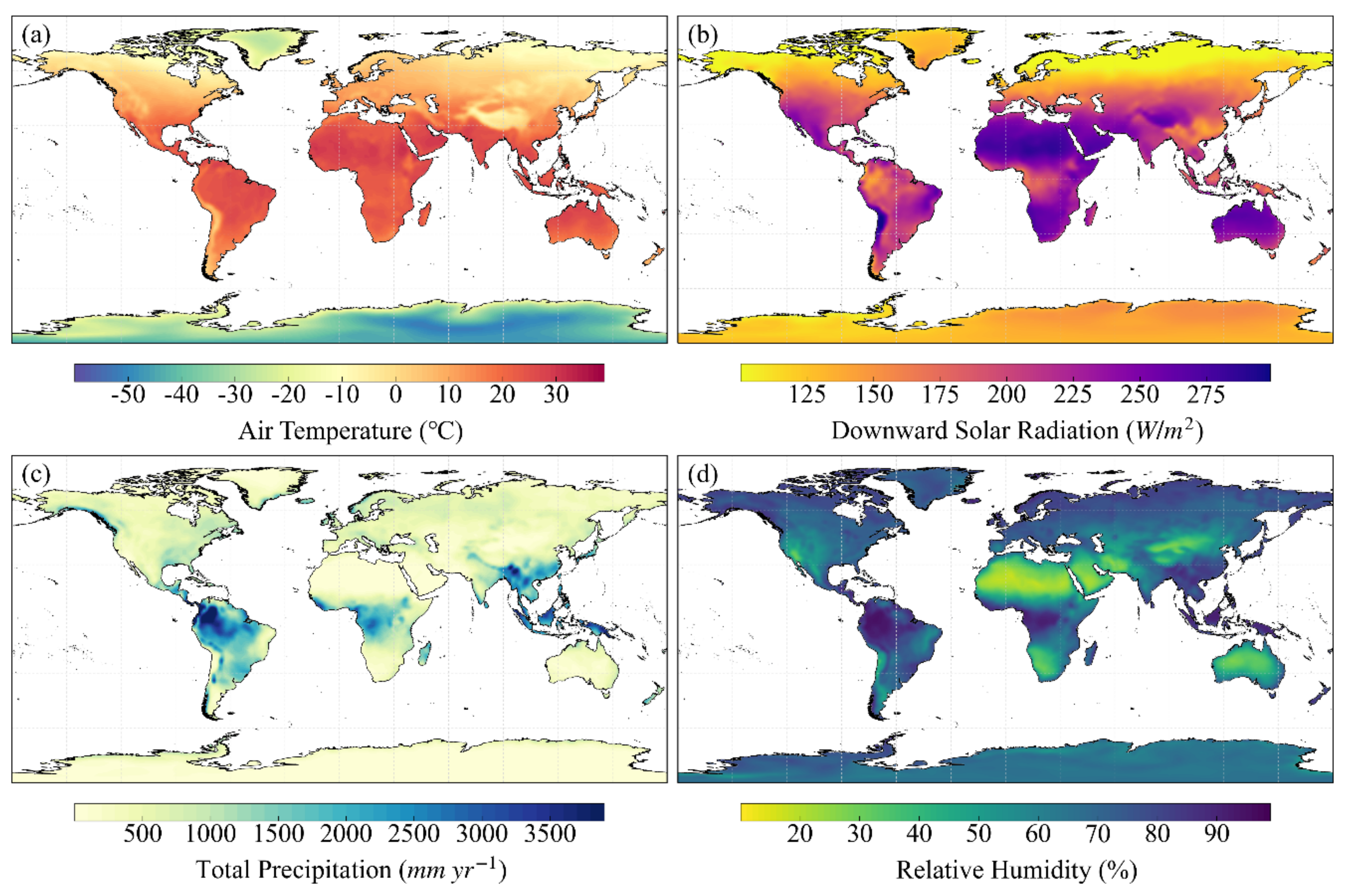
3.1. Meteorological Data

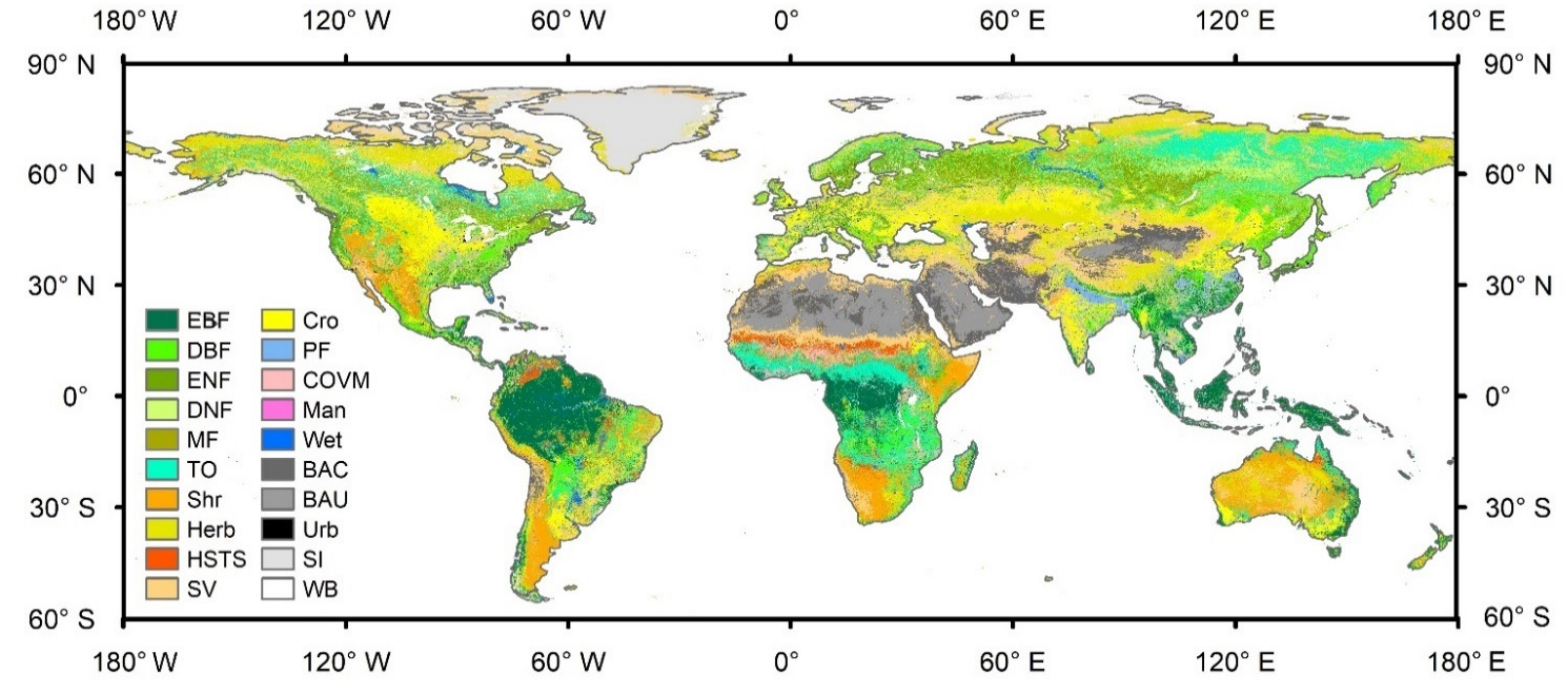
The gridded meteorology data include downward solar radiation, two-meter T_a, RH, rainfall (Figure 1), and ten-meter wind speed, and they are downloaded from the ERA-Interim Archive at the European Centre for Medium-Range Weather Forecasts (ECMWF). The data assimilation system used for producing ERA-Interim was based on a 2006 release of the Integrated Forecast System (Cy31r2). This data assimilation system includes a 4-dimensional variational analysis (4D-Var) with a 12-hour analysis window [47]. The data assimilation performance has been closely monitored during the production of ERA-Interim [47]. The spatial resolution of this dataset is approximately 80 km (~1°). For hourly simulation at a 1° resolution, the cubic spline interpolation method in Matlab was applied to interpolate ERA-interim meteorology data from three hourly to one hourly.

3.2. Land Cover Map

Global land cover (LC) map in 2013 at 500 m resolution from the Global Land Cover by National Mapping Organizations (GLCNMO) (https://globalmaps.github.io/glcnm-o.html, accessed on 3 July 2021) is used in this study. There are 19 LC types based on the Land Cover Classification System (LCCS) [48] (Figure 2). For global ET simulation, the detailed LC types were lumped into nine PFTs. Specifically, EBF, DBF, ENF, DNF, MF, and shrub are kept as they are. Herbaceous is labeled as grass. Cropland, paddy field, and Cropland/Other Vegetation Mosaic were labeled as crop. Other LC types in Figure 1 were labeled as others. For each 1° modeling pixel, the areal fraction of each PFT was calculated to upscale from 500 m to 1° resolution [49].

In this study, the BEPS model was run at 1° resolution for ET simulation. Thus, the GLCNMO global land cover map at 500 m resolution is good enough for this study. The latest GLCNMO land cover map available online is the Version 3 data which was produced from the MODIS data in 2013. This is the reason why we used the GLCNMO2013 land cover map. There is only two years’ difference between 2015 and 2013 and the changes of land cover types should be minor within two years. Thus, we assumed that this global land cover map in 2013 could still be used for our ET simulation in 2015.

3.3. Global LAI Product

The global LAI product in 2015 used in this study was retrieved from the GLOBMAP LAI Version 3 dataset, which includes consistent long-term (1981–2019) global LAI maps at 8 km resolution [37]. The global LAI maps in 2015 were derived from 8-day synthesis MODIS land surface reflectance products (MOD09A1 C6) and the angular information. The red, near-infrared (NIR), and shortwave-infrared (SWIR) reflectance were used for LAI derivation based on the GLOBCARBON LAI algorithm. The cloud pixels of MOD09A1 C6 data were identified by an algorithm of cloud detection [50], and the cloud pixels were filled using the approach of locally adjusted cubic spline capping [51]. The leaf clumping effects had been considered for each pixel with a global CI map at 500 m resolution [52]. This global LAI product had been validated using field measurements of 28 sites and 45 LAI maps of fine resolution over 29 sites which covered major global PFTs [37]. A global LAI map on 4–11 July 2015, is shown as an example in Figure 3.

For ET modeling at the one-degree resolution, the global LAI maps at 8 km resolution were aggregated to derive the mean LAI value for each PFT in each one-degree grid. In this approach, each PFT within the one-degree grid is considered, and the LAI related to each specific PFT is averaged from all the fine resolution pixels. This allowed separate ET estimation for each PFT in each one-degree grid. The ET value of each one-degree grid was then calculated as the sum of ET for all PFTs weighted by their areal fractions [49].

3.4. Global Clumping Index Map

CI is a key canopy structural parameter quantifying the level of leaf clumping in vegetation canopy. Chen et al. (2005) firstly proposed the Normalized Difference between Hotspot and Darkspot (NDHD), which is an improved angular index for deriving the global CI map with multi-angular remote sensing data at 6 km resolution [53]. In this study, we used a global CI product (hereafter CAS-CI) at 500 m resolution in 2015, which was derived from the MODIS BRDF product [27]. This is currently the finest global CI map of which temporal resolution is 8-day (Figure 4). This global CI map has been validated with in-situ observations of CI at thirty-three sites [27]. This global CI map series was aggregated to derive the mean CI value for each PFT in each 1° grid and it was the basis for the assessment of the impacts of leaf clumping on global ET simulation.

3.5. Soil Texture Data

The soil texture type for each one-degree pixel was determined by the sand, silt, and clay fractions. The soil texture data were downloaded from the Harmonized World Soil Database (HWSD) (http://webarchive.iiasa.ac.at/Research/LUC/External-World-soil-database/HTML/HWSD_Data.html?sb=4, accessed on 3 July 2021). The spatial resolution of the original HWSD dataset is 0.00833 degrees (~1 km) and they were resampled into grids of 0.004167° (~500 m) to match the spatial resolution of the global LC map. The soil texture type of each grid cell was determined by the USDA soil texture triangle and the sand, silt, and clay fractions.

For global ET simulation at 1° resolution, the soil texture map at 500 m resolution was aggregated to obtain the dominant soil texture types for the 9 PFTs (Section 3.2). The soil texture types were used to determine the soil hydrological and thermal parameter values such as saturated hydraulic conductivity, porosity, field capacity, wilting point, and soil thermal conductivity, which would influence the estimation of soil evaporation through the ground surface temperature and soil moisture.

4. Simulation Cases and Model Validation

For the purpose of investigating leaf clumping effects on the estimated global ter-restrial ET, three cases of model simulations were conducted. For Case I, both of the true LAI and CI retrieved from remote sensing data were used. This Case was believed to be unbiased. For Case II, the true LAI was used but clumping was ignored (CI = 1). This case would cause the overestimation of sunlit LAI and the underestimation of shaded LAI compared to Case I. For Case III, the effective LAI (L_e) calculated as the product of remote sensing true LAI (GLOBMAP LAI) and remote sensing CAS-CI was used and clumping was ignored. In this case, the sunlit LAI is not biased but the shaded LAI is underestimated compared to Case I. The BEPS simulated soil moisture (SM) from Case I was used to drive the other case simulations for removing the effects of simulated SM on simulated ET among different cases.

The BEPS model simulated ET has been validated extensively with the eddy-covariance (EC) measured ET for C3 and C4 crops in the Western Lake Erie Basin, the USA [54], boreal and temperate forest ecosystems in North America [11,14,55], forest, grassland and cropland in China [56,57,58]. In these studies, the BEPS model simulated half-hourly ET was compared with the EC measured ET and the R² is in the range of 0.43 to 0.86 and the RMSE ranging from 0.02 to 0.08 mm hr⁻¹. The Penman-Monteith equation used to estimate ET and the two-leaf model used to upscale ET from leaf-level to canopy scale have been proved to perform better than their alternatives [11,59]. Thus, the global terrestrial ET simulated by the BEPS model in this study should be reasonable as long as the uncertainties from the input dataset could be well-constrained.

5. Results

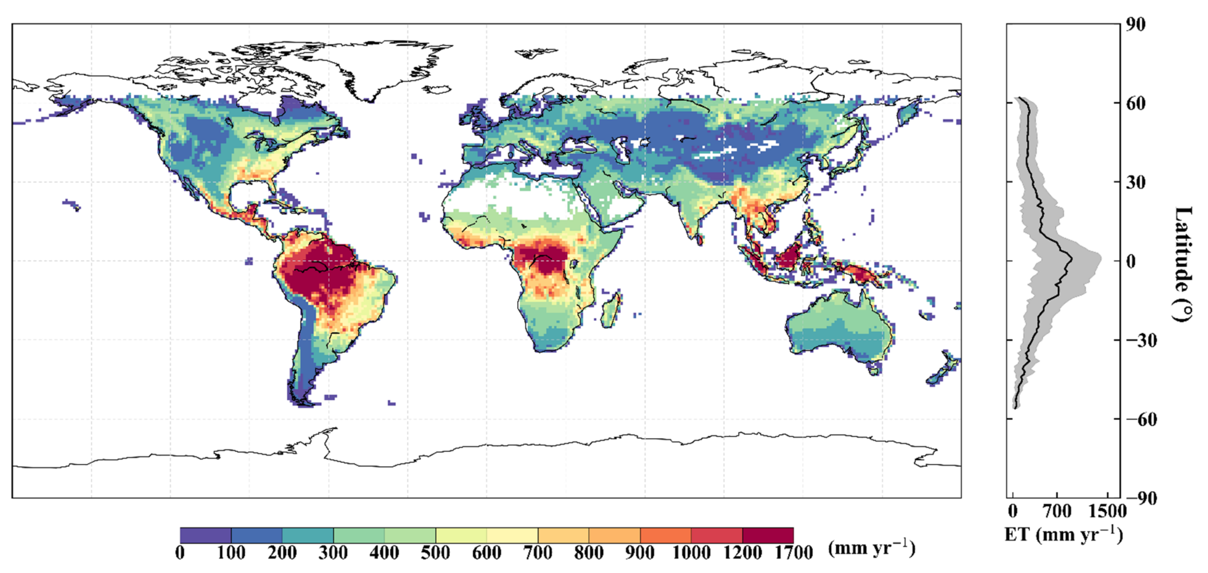
5.1. Simulations of Global Terrestrial ET

Using the various land cover, meteorology, and soil inputs, a global annual ET map for 2015 is produced at one-degree resolution for each of the three cases, based on the hourly BEPS simulation. The global ET map of Case I is considered as representing the reality (Figure 5). The highest ET appeared in the tropics while low ET appeared in the northern high latitudes, high-altitude mountains, and arid regions (i.e., Australia, central Asia, the western US, and the Sahel). The mean ET variations with latitude are also shown in Figure 4. The highest ET (933.4 ± 472.5 mm yr⁻¹) occurs at the latitude of 1°N and ET gradually decreases with the increase of latitude to the North or the South (Figure 5). The variation of annual ET with latitude is large due to strong latitudinal variations in meteorological conditions, vegetation types, and densities.

The ET averaged over the global land surface is 511.9 ± 70.1 mm yr⁻¹, where the uncertainty ± 70.1 mm yr⁻¹ is the sum of the uncertainty (±26.7 mm yr⁻¹) resulting from the input vegetation data as well as model parameters, and the standard deviation (±43.4 mm yr⁻¹, Figure 8) of the annual global ET during 2013 to 2016 resulting from meteorological variations. The uncertainty from meteorological variations is calculated using the same model parameters and the same LAI and CI input dataset in 2015 but actual hourly meteorological data from 2013 to 2016. The uncertainty resulting from the input vegetation data and model parameters is approximated by the range of global terrestrial ET variation caused by LAI uncertainty of 20% (see

Table 2. Sensitivities of global terrestrial ET (mm yr⁻¹) to errors in key parameters such as LAI, Ω, $V_{cmax0}^{25}$, and $RAS{M}_{th}$.

	Case I a	Case II	Case III	Case II–Case I b	Case III–Case I b
Baseline c	511.9	535.9	445.6	24.0 (4.7%)	−66.3 (−13.0%)
1.2*LAI	541.6 (5.8%)	565.0	473.9	23.4 (4.3%)	−67.7 (−12.5%)
0.8*LAI	476.6 (−6.9%)	501.1	413.3	24.6 (5.2%)	−63.3 (−13.3%)
1.2*Ω	521.6 (1.9%)	535.9	476.4	14.3 (2.7%)	−45.3 (−8.7%)
0.8*Ω	499.1 (−2.5%)	535.9	409.9	36.8 (7.4%)	−89.2 (−17.9%)
$1.2*V_{cmax0}^{25}$	525.2 (2.6%)	551.6	458.7	26.4 (5.0%)	−66.5 (−12.7%)
$0.8*V_{cmax0}^{25}$	494.5 (−3.4%)	515.9	429.1	21.4 (4.3%)	−65.4 (−13.2%)
1.2*RASMth	503.7 (−1.6%)	526.0	437.5	22.3 (4.4%)	−66.2 (−13.1%)
0.8*RASMth	522.6 (2.1%)	548.5	456.1	25.9 (5.0%)	−66.6 (−12.7%)

^a The percent in the parentheses of the 2nd column represents RD to the baseline ET. ^b The percent in the parentheses of the last two columns represents RD to ET of Case I. ^c The baseline is the ideal Case shown in Figure 7.

) [23].

5.2. Spatial Patterns of Leaf Clumping Effects on ET Estimation

Compared to Case I, leaf clumping effects on global terrestrial ET simulation are assessed. The spatial patterns of bias errors for ET estimates among cases have consistent signs, either positive (Figure 6) or negative (Figure 7), indicating that the clumping effects are spatially consistent, despite considerable differences in other variables such as meteorology, plants, and soils. It means that leaf clumping effects are vital for the two cases. The largest biases due to neglecting leaf clumping exist in the tropical and the boreal forests (Figure 6 and Figure 7) where high clumping is detected from the MODIS BRDF product (Figure 4). Figure 6 demonstrates that the ET values are overestimated globally if true LAI is used ignoring clumping. The reason is that overstory sunlit LAI is overestimated in Case II. Leaf clumping leads to more light penetration into the canopy and a decrease in overstory sunlit LAI. If ignoring clumping, overstory sunlit LAI would be positively biased while overstory shaded LAI would be negatively biased. Because ET of sunlit leaves is larger than that of shaded leaves per unit leaf area, the total ET is positively biased for Case II.

Figure 7 demonstrates the converse effects of leaf clumping globally for Case III. It can be found that the detailed spatial distributions of the leaf clumping effects are relatively different in Figure 6 and Figure 7. In Case II (Figure 6), the high clumping effects on ET do not appear where LAI is large. The reason is that the relative change in overstory shaded LAI with CI is larger at lower LAI values while the absolute value of overstory shaded LAI varies little with LAI (Equations (9) and (10)). In Case III (Figure 7), the high clumping effects appear in areas with high LAI. This is because the overstory shaded LAI would be more negatively biased with larger LAI values when the CI is the same.

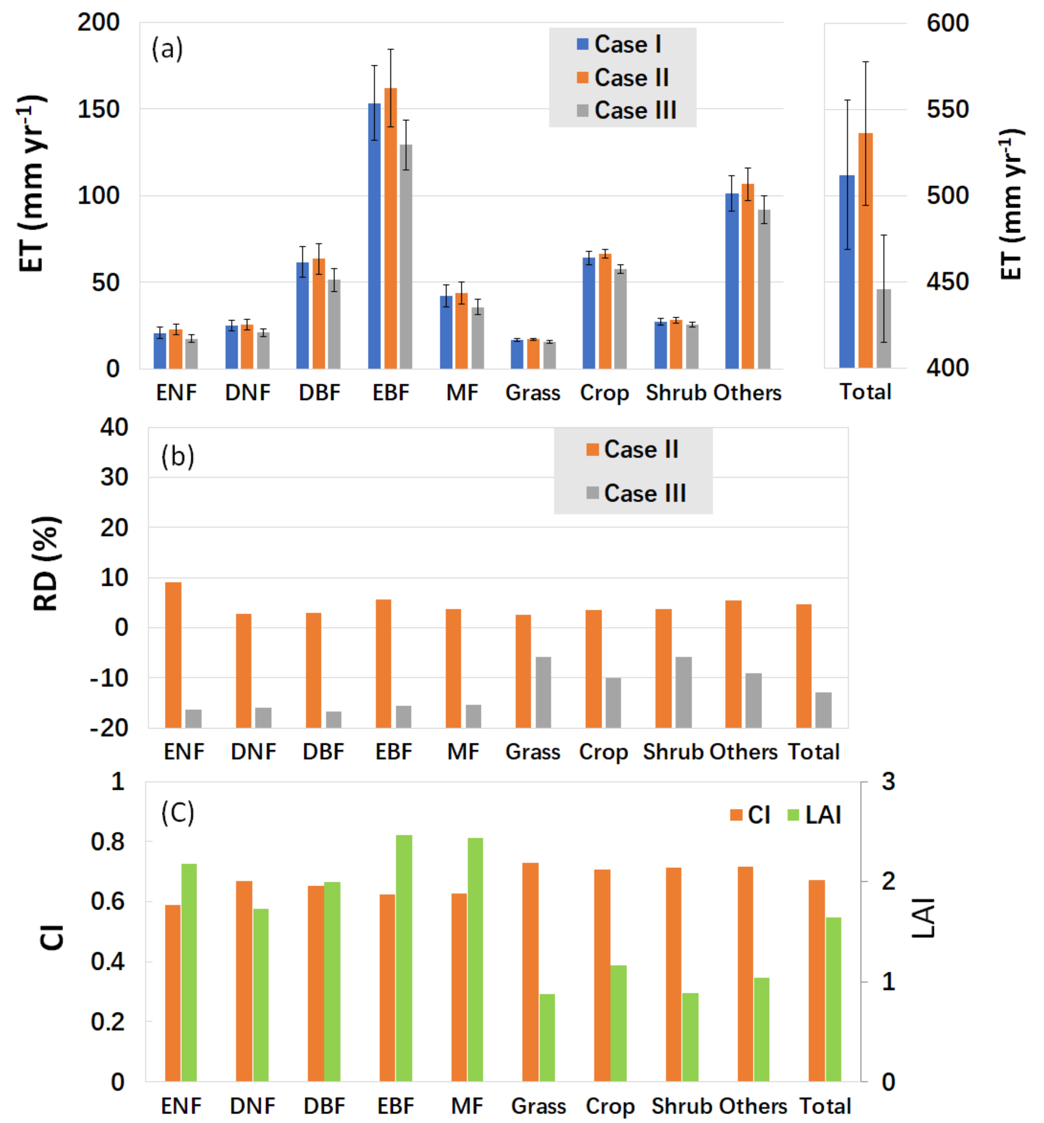
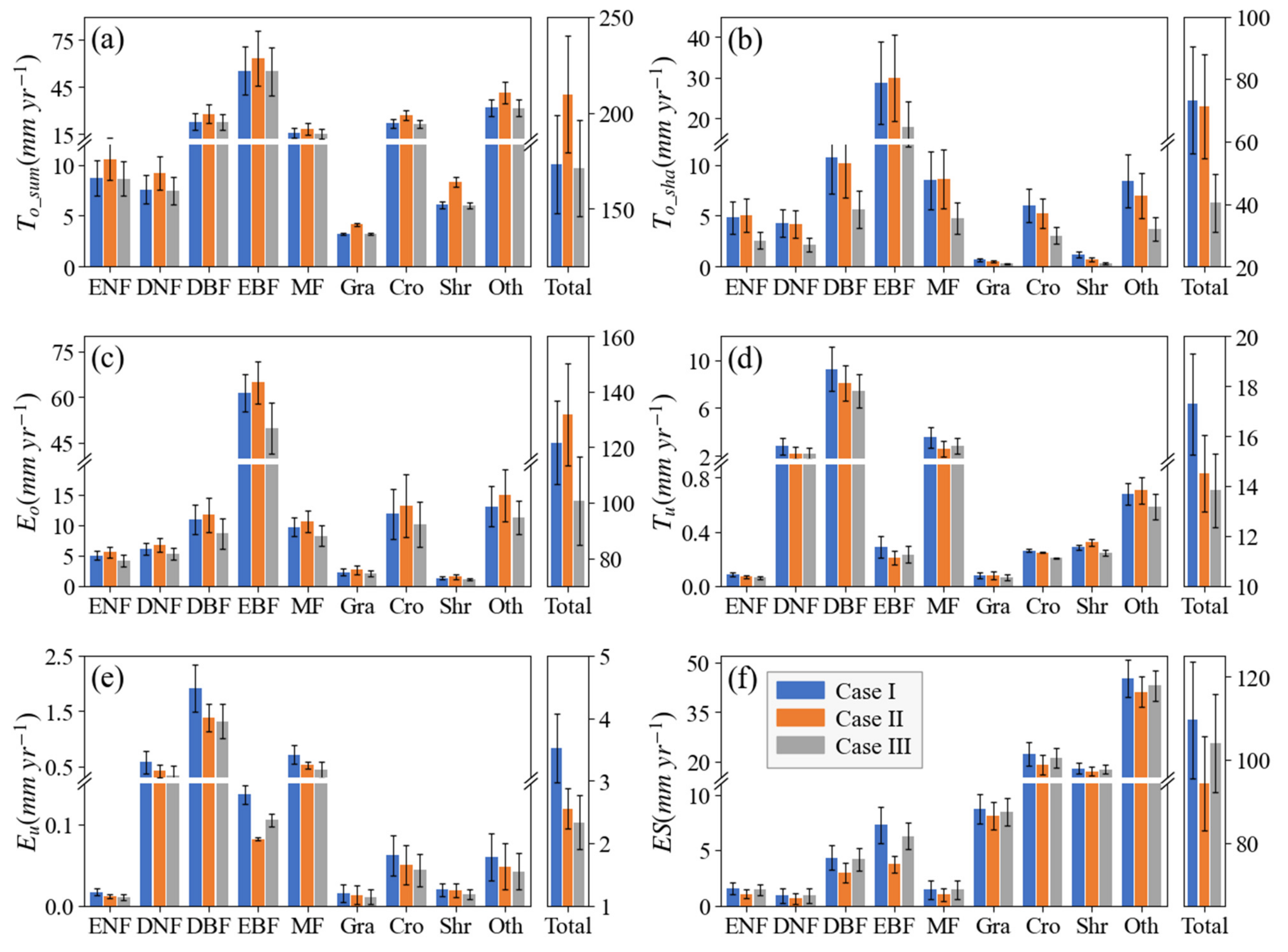
5.3. Leaf Clumping Effects on ET Estimation and Its Components for Various PFTs

Based on Case I, leaf clumping effects on estimations of global terrestrial ET as well as its components have been assessed for various PFTs (Figure 8). The discrepancy of ET is 18.3 mm yr⁻¹ (4.7%) between Case II and Case I and −48.3 mm yr⁻¹ (−13.0%) between Case III and Case I (Figure 8). ET of Case II is always larger than those of Case I for all PFTs (Figure 8). Evergreen needleleaf forests (ENF) have the largest relative differences (RD) between Case II and Case I because they are most clumped with the lowest CI on average (Figure 8).

In contrary to Case II, ET is underestimated for all PFTs in Case III. The reason is that the effective LAI of a highly clumped canopy is much smaller than its true LAI. Deciduous broadleaf forests (DBF) have the largest RD between Case III and Case I because DBF has both high LAI and low CI compared to other PFTs (Figure 8). If effective LAI is used ignoring clumping, shaded LAI is much smaller in Case III than that in Case I, especially for high LAI and low CI, while the sunlit LAI is unchanged (Equation (9)). Thus, the ET of shaded leaves in Case III is lower than those in Case I so that the total ET is underestimated for Case III.

ET of Case III is underestimated considerably due to the large fractions of shaded T_o in ET. The fractions of shaded T_o to total ET are 23.2%, 17.0%, 17.3%, 18.7%, 20.1%, 4.1%, 9.4%, 4.4% and 8.3% to ET for ENF, DNF, DBF, EBF, MF, grass, crop, shrubs and others. The discrepancy in ET between Case III and Case I is more than that between Case II and Case I because ET is more biased due to the underestimation of shaded LAI in Case III than that caused by the overestimation of sunlit LAI in Case II. This is consistent with what Chen et al. [14] found by assessing leaf clumping effect on ET estimates over eight forest sites in North America.

Leaf clumping effects on ET components of the various PFTs were further investigated in Figure 9. Overstory sunlit transpiration (T_{o_sun}) values of Case II are always higher than those of Case I (Figure 9a) because overstory sunlit LAI is overestimated in Case II. Overstory shaded transpiration (T_{o_sha}) values of Case II are all close to those of Case I (Figure 9a). This is because the overestimation of leaf-level T_{o_sha} is offset by the underestimation of overstory shaded LAI in Case II. T_{o_sun} values of Case III are almost the same as those of Case I (Figure 9a) because both leaf-level T_{o_sun} and overstory sunlit LAI are unchanged in Case III. T_{o_sha} values of Case III are always lower than those of Case I (Figure 9b) because the underestimation of overstory shaded LAI is more significant than the overestimation of leaf-level T_{o_sha} in Case III. E_o values of Case II are always higher than those of Case I while E_o values of Case III are always lower than those of Case I (Figure 9c). T_u values of Case II and Case III are both lower than those of Case I for most of the PFTs (Figure 9d). E_u and ES values of Case II and Case III are both lower than those of Case I for all the PFTS (Figure 9e,f).

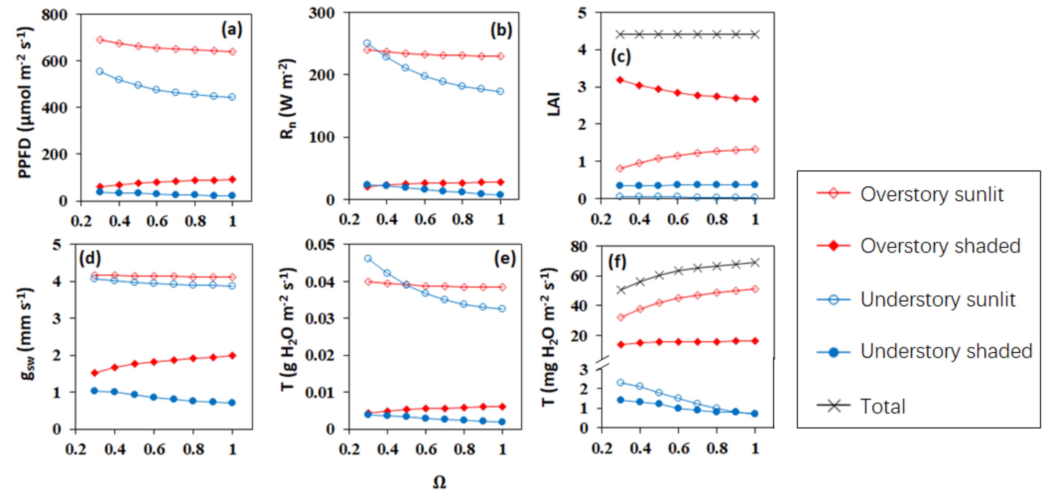
5.4. Leaf Clumping Effects on the Calculation of Key Biophysical Parameters Controlling Transpiration Simulations

In this section, we explored leaf clumping effects on the calculation of key biophysical parameters controlling transpiration (T) estimation, which is the major component of ET, such as leaf-level absorbed photosynthetic photon flux density (PPFD), net radiation (R_n), stomatal conductance to water vapor (g_sw) and LAI. The leaf clumping effects on the calculation of these biophysical parameters were investigated for sunlit and shaded leaves in the overstory and understory canopies, respectively (Figure 10 and Figure 11).

If true LAI is used in transpiration estimation and clumping is ignored, leaf-level absorbed PPFD, Rn, g_sw, and T of the representative sunlit leaf in the overstory canopy would be negatively biased (Figure 10a,b,d,e). In contrast, leaf-level absorbed PPFD, R_n, g_sw, and T of the shaded leaf in the overstory canopy would be positively biased when true LAI is used in transpiration calculation and clumping is ignored (Figure 10a,b,d,e). For instance, in a typical conifer forest, where LAI is 4.0 and Ω is 0.5, downward shortwave radiation above the canopy is 500 W m⁻² and relative humidity is 80%, leaf-level absorbed PPFD, R_n, g_sw, and T of the representative sunlit leaf in the overstory canopy would be 663.7 ${\mathsf{\mu }\mathrm{mol} \mathrm{m}}^{-2}{\mathrm{s}}^{-1}$, 234.3 W m⁻², 4.15 mm s⁻¹ and 0.0391 g H₂O m⁻² s⁻¹ when clumping is considered (Figure 9). However, they will be 641.0 ${\mathsf{\mu }\mathrm{mol} \mathrm{m}}^{-2}{\mathrm{s}}^{-1}$, 229.8 W m⁻², 4.12 mm s⁻¹, and 0.0384 g H₂O m⁻² s⁻¹ when clumping is ignored (Figure 9). Thus, the relative errors (RE) in the estimations of leaf-level absorbed PPFD, Rn, gsw, and T for the representative sunlit leaf in the overstory canopy are −3.4%, −1.9%, −0.6%, and −1.8% when clumping is ignored. In this case, leaf-level absorbed PPFD, Rn, gsw and T of the representative shaded leaf in the overstory canopy would be 75.8 ${\mathsf{\mu }\mathrm{mol} \mathrm{m}}^{-2}{\mathrm{s}}^{-1}$, 24.3 W m⁻², 1.76 mm s⁻¹ and 0.0053 g H₂O m⁻² s⁻¹ when clumping is considered (Figure 10). However, they will be 91.9 ${\mathsf{\mu }\mathrm{mol} \mathrm{m}}^{-2}{\mathrm{s}}^{-1}$, 27.9 W m⁻², 1.98 mm s^−1, and 0.0061 g H₂O m⁻² s⁻¹ when clumping is ignored (Figure 10). Thus, the relative errors in the estimations of leaf-level absorbed PPFD, Rn, gsw, and T for the representative shaded leaf in the overstory canopy are 21.2%, 14.7%, 12.8%, and 15.1% when clumping is ignored. The positive biases in these variables for the shaded leaf in the overstory are much higher than the negative biases for the sunlit leaf in the overstory.

In this case, leaf-level absorbed PPFD, Rn, gsw, and T for understory sunlit and shaded leaves would be negatively biased when true LAI is used in transpiration estimation and clumping is ignored (Figure 10). Meanwhile, understory sunlit LAI would be negatively biased while understory shaded LAI would be positively biased when true LAI is used in transpiration calculation and clumping is ignored (Figure 10). In this case, canopy-scale understory sunlit and shaded T would be both negatively biased (Figure 10f).

For the same L_e, the overstory or understory shaded LAI as well as total LAI increased with the decrease of Ω (more clumped) while overstory or understory sunlit LAI were invariant (Figure 11c). When L_e is used in estimating T ignoring clumping, leaf-level absorbed PPFD, R_n, g_sw, and T of the overstory representative sunlit leaf were invariant while those of the overstory representative shaded leaf were overestimated (Figure 11). Canopy-level overstory sunlit T was invariant while the shaded T and total T were negatively biased when effective LAI is used ignoring clumping (Figure 11f).

Using the same example as mentioned above, effective LAI for the overstory and understory canopies are set as a constant of 2.0 and 0.2, respectively. If Ω is 0.5, absorbed PPFD, R_n, g_sw and T for the overstory representative shaded leaf at $\theta =45°$ is 75.8 ${\mathsf{\mu }\mathrm{mol} \mathrm{m}}^{-2}{\mathrm{s}}^{-1}$, 24.3 W m⁻², 1.76 mm s⁻¹ and 0.0053 g H₂O m⁻² s⁻¹, respectively, when clumping is considered, while they are 155.7 ${\mathsf{\mu }\mathrm{mol} \mathrm{m}}^{-2}{\mathrm{s}}^{-1}$, 42.5 W m⁻², 2.64 mm s⁻¹ and 0.0089 g H₂O m⁻² s⁻¹, if clumping is ignored (Figure 11). The RE in the estimation of PPFD, R_n, g_s,w, and T when clumping is ignored will be 105.3%, 74.8%, 50.0%, and 67.9%, for the overstory representative shaded leaf. Meanwhile, the sunlit LAI in overstory and understory are unchanged and the shaded LAI in overstory and understory were negatively biased by 68.2% and 56.3% (Ω = 0.5). Total LAI was underestimated by 50.0% if Ω is 0.5 (Figure 11c). Accordingly, T of the overstory sunlit canopy would be unchanged while that of the shaded counterpart was underestimated by 46.8% (Figure 11f). On the other hand, T of understory sunlit canopy would be underestimated by 11.1% while that of the shaded counterpart was underestimated by 33.3%. The total canopy-level transpiration rate was underestimated by 13.6% in this Case (Figure 11f).

6. Discussion

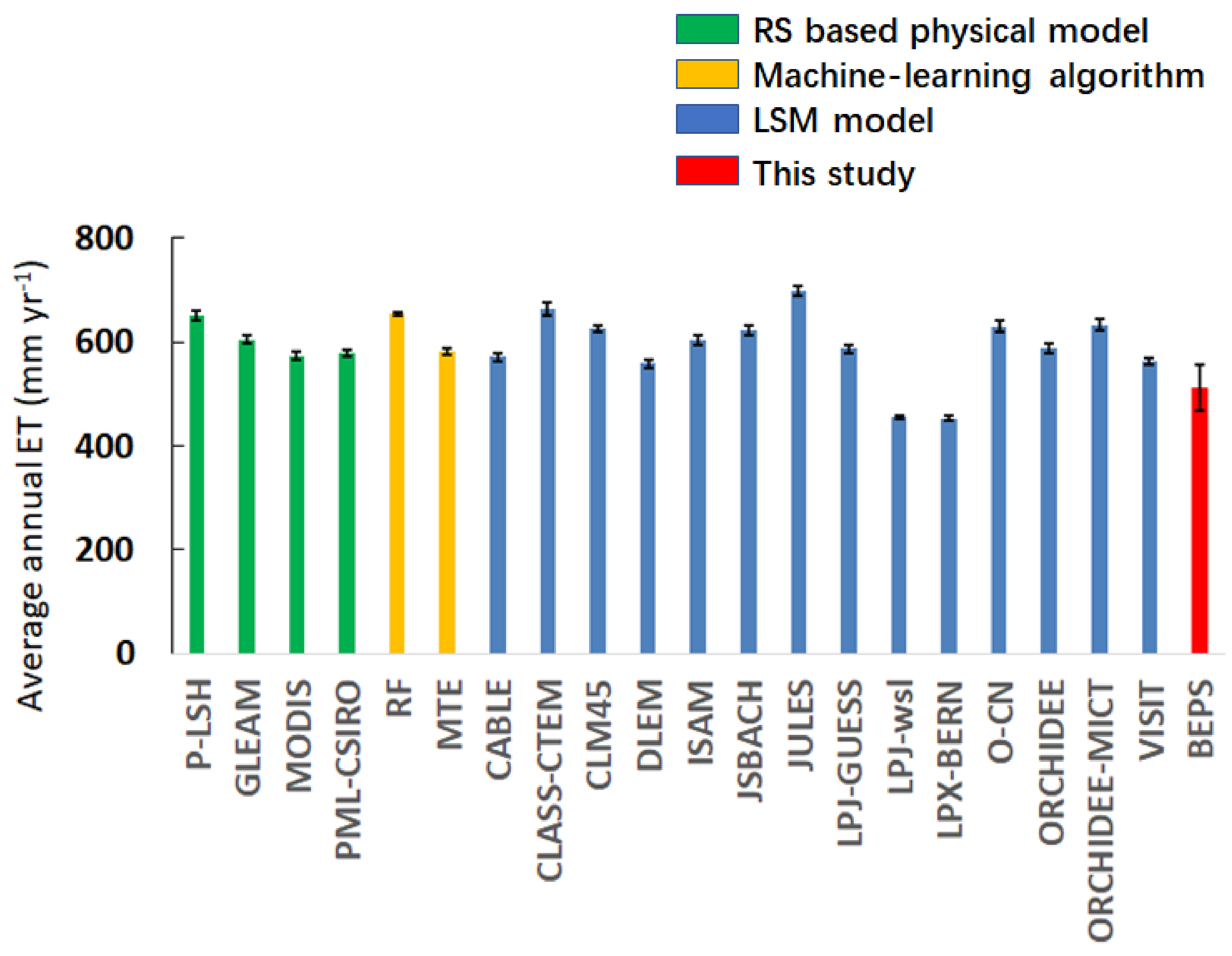
6.1. Estimations of Global Terrestrial ET

The multiyear average of annual global terrestrial ET (511.9 ± 43.4 mm yr⁻¹) from 2013 to 2016 simulated by the BEPS model in this study is within the range (453.7 ± 5.2 to 697.3 ± 10.4 mm yr⁻¹) of those estimated by four remote sensings (RS) based physical models, two machine learning methods (i.e., model tree ensemble and random forest), and 14 land surface models (LSM) (Figure 12) [1]. For the model tree ensemble (MTE) method, eddy covariance (EC) measured ET was integrated with satellite remote sensing and surface meteorological data to estimate global terrestrial ET monthly from 1982 to 2008 at 0.5° spatial resolution [60]. For the random forest (RF) algorithm, a set of independent regression trees was generated by randomly selecting training samples automatically [61]. The RF global terrestrial ET product has a temporal resolution of half-hourly for the period of 2001–2014 at 0.5 spatial resolution [62]. The 14 LSM modeled ET products were from Trends and Drivers of the Regional Scale Sources and Sinks of Carbon Dioxide (TRENDY) project, including CABLE, CLASS-CTEM, CLM45, DLEM, ISAM, JSBACH, JULES, LPJ-GUESS, LPJ-wsl, LPX-BERN, O-CN, ORCHIDEE, ORCHIDEE-MICT and VISIT [1]. The global terrestrial ET results from the S3 simulation of TRENDY v6 with changing CO₂, climate, and land use for the period of 1982–2011 were used for comparison in this study. The interannual variability of global terrestrial ET from 1982 to 2011 is small (<13.0 mm yr⁻¹) [1]. Thus, the magnitude of global terrestrial ET simulated by the BEPS model in this study is reasonable although its period is different from that in Pan et al. [1].

6.2. Sensitivities of ET to Errors in Key Parameters of the BEPS Model

Uncertainties in the global ET estimation resulting from errors in key model parameters might be as large as the impacts of leaf clumping mentioned above. To investigate the robustness of our results on the impacts of leaf clumping on global ET estimation, sensitivity analysis was conducted for four key parameters such as LAI, $\mathsf{\Omega }$, V_cmax, and the threshold of relatively available soil moisture under which soil water stress occurs (RASM_th). If LAI is uniformly increased or reduced by 20% (assessed LAI error), ET is increased by 6.0% or reduced by 7.0% (Table 2). Nevertheless, the relative differences (RD) between Case II and Case I and between Case III and Case I are affected slightly (less than 0.5%) by the variations in LAI. This indicated that all cases are influenced by the LAI changes in the same direction. Similar to LAI, if $V_{cmax0}^{25}$ is increased or reduced by 20% in the BEPS model, global terrestrial ET would be increased or decreased in similar magnitudes (around 3.0%), but RD between the cases representing leaf clumping effects changed very little (<0.5%). When $RAS{M}_{th}$ is increased or reduced by 20%, global terrestrial ET is decreased by 1.6% or increased by 2.1%, but the RD between the cases changed very little (<0.5%). Generally, if other parameters in the BEPS model (i.e., N₀ and m in Table 1) are modified, the three cases would be moved in the same direction, and the leaf clumping effects quantified as the RD in global terrestrial ET between the cases would not be considerably influenced by these changes. These sensitivity tests support the justification of the spatially consistent leaf clumping effects (Figure 6 and Figure 7).

In line with expectations, if Ω is increased or reduced by 20%, the RD among the cases would be changed substantially (Table 2). In the initial evaluation with field measurements, the average bias error of the CAS-CI product was around 0.01 (~2%) and nearly all CAS-CI values were located within $\pm 0.1$ of the field observations [27]. Therefore, the 20% variation is generous for most PFTs. The variation range has been made large for covering the high uncertainty in CI estimation of tropical forests [23]. Although leaf clumping is decreased by 20% (Ω is increased), there is still a 2.7% difference between Case II and Case I, 7.4% difference between Case III and Case I, indicating that leaf clumping effects should not be neglected even though substantial uncertainties still exist in Ω measurements.

6.3. Implications and Uncertainties of This Study

For ET estimation, both LAI and Ω are required for describing complex canopy architecture. Both LAI and Ω can be acquired from remote sensing. Nevertheless, there are still uncertainties in the values of the two parameters. By now, several global LAI products with moderate resolution (250 m to 7 km) are available based on different algorithms [63]. Depending on field measurements and models used in the algorithm, some LAI products are close to L_e [64,65] while some are close to true LAI [7,37,66]. If field-measured LAI is based on allometric equations or acquired from destructive sampling, the LAI would be close to true LAI. If optical instruments (i.e., LAI-2200 or DHP) are used to measure LAI without the clumping correction, the LAI is effective LAI [23]. Some remote sensing LAI products (i.e., GA-TIP and JRC-TIP) were produced based on data assimilation retrieval from albedo without the clumping collection, and thus they are effective LAI instead of the true LAI [63]. Clumping correction is needed for these LAI products before they are used for global ET simulation.

Although the GLOBMAP LAI product used in this study has incorporated the leaf clumping effects, there are still biases in the global CI map used for the GLOBMAP LAI production due to using the RossThick-LiSparse Reciprocal (RTLSR) model with a constant $\theta$ of 0° [37,52]. CI of slight to middle clumped canopies was underestimated while they were overestimated for sparsely vegetated areas by this BRDF and SZA configuration [39]. The CAS-CI product performed better than the CI product produced by He et al. [52], and it has a lower bias when validated with ground measurements. However, the CAS-CI product does not perform well over very sparse crop sites due to the substantial impacts of exposed soil, which impair the derivation of CI from remote sensing data using the NDHD method [27,39]. Moreover, the NDHD method has a disadvantage of underestimating the true CI for tropical forests as satellite sensors are majorly detecting the thick overstory canopy, which would keep off the understory canopy [67]. The influences of frequent clouds would also impair the CI retrievals over tropical areas [27].

There are only a few CI validations for extremely sparse and dense vegetation conditions [27]. Thus, in the spatial patterns of leaf clumping effects on ET, the largest uncertainties would exist in these areas. More field observations are required for further evaluation of the CI estimation over these land cover types. Shrubs and other vegetation types would also have large uncertainties as these PFTs have not been extensively validated in the BEPS model.

7. Conclusions

The significance of leaf clumping to global terrestrial ET simulation is revealed from its influences on sunlit and shaded LAI stratification, on the calculation of true LAI from effective LAI, and estimations of leaf-level irradiance. This is the first time that foliage clumping effects on ET estimation are assessed globally. The following main conclusions are drawn from this study:

• Even though accurate global LAI data is used, neglecting leaf clumping will overestimate global terrestrial ET by about 4.7%. The reason is that leaf clumping reduces sunlit LAI while increases shaded LAI, resulting in an overall reduction in ET.
• If L_e is used, neglecting leaf clumping will underestimate global terrestrial ET by 13.0%. The reason is that L_e is lower than true LAI for a clumped canopy. If L_e instead of true LAI is used in ET simulation ignoring leaf clumping impacts, shaded LAI would be substantially negatively biased while sunlit LAI is invariant, causing negative bias in ET.
• Although the accuracy of global terrestrial ET simulation still needs improvements, leaf clumping impacts quantified by the RDs between the model simulation cases considering or ignoring clumping are still robust since errors of key model parameters will move in the same directions for all cases.

This study highlights the importance of considering leaf clumping in estimating global terrestrial ET, which would be helpful to improve the quality of global terrestrial ET products derived from various land surface models. Both LAI and CI are needed for accurately estimating sunlit and shaded LAI as well as ET by the two-leaf model. This two-leaf separately ET estimation is important because stomatal conductance controlling transpiration is coupled with photosynthesis at leaf-level, of which sunlit and shaded leaves are controlled by different biochemical processes.

For better serving the global water research, the remote sensing community should produce more accurate global CI products based on data from new satellite sensors. Physical retrieval methods should also be explored to produce high-resolution global CI products. Finally, more field measurements are also needed for the validation of global CI products, especially in tropical regions.

References

1. Pan, S.; Pan, N.; Tian, H.; Friedlingstein, P.; Sitch, S.; Shi, H.; Arora, V.K.; Haverd, V.; Jain, A.K.; Kato, E.; et al. Evaluation of global terrestrial evapotranspiration using state-of-the-art approaches in remote sensing, machine learning and land surface modeling. Hydrol Earth Syst Sci. 2020, 24, 1485–1509. [Google Scholar] [CrossRef] [Green Version]
2. Jasechko, S.; Sharp, Z.D.; Gibson, J.J.; Birks, S.J.; Yi, Y.; Fawcett, P.J. Terrestrial water fluxes dominated by transpiration. Nature 2013, 496, 347–350. [Google Scholar] [CrossRef] [PubMed]
3. Oki, T.; Kanae, S. Global hydrological cycles and world water resources. Science 2006, 313, 1068–1072. [Google Scholar] [CrossRef] [PubMed] [Green Version]
4. Trenberth, K.E.; Fasullo, J.T.; Kiehl, J. Earth’s global energy budget. Bull Am. Meteorol. Soc. 2009, 90, 311–312. [Google Scholar] [CrossRef]
5. Lian, X.; Piao, S.; Huntingford, C.; Li, Y.; Zeng, Z.; Wang, X.; Ciais, P.; McVicar, T.R.; Peng, S.; Ottlé, C.; et al. Partitioning global land evapotranspiration using CMIP5 models constrained by observations. Nat. Clim. Chang. 2018, 8, 640–646. [Google Scholar] [CrossRef]
6. Sellers, P.J.; Dickinson, R.E.; Randall, D.A.; Betts, A.K.; Hall, F.G.; Berry, J.A.; Collatz, G.J.; Denning, A.S.; Mooney, H.A.; Nobre, C.A.; et al. Modeling the Exchanges of Energy, Water, and Carbon Between Continents and the Atmosphere. Science 1997, 275, 502–509. [Google Scholar] [CrossRef] [PubMed] [Green Version]
7. Yan, H.; Wang, S.Q.; Billesbach, D.; Oechel, W.; Zhang, J.H.; Meyers, T.; Martin, T.A.; Matamala, R.; Baldocchi, D.; Bohrer, G. Global estimation of evapotranspiration using a leaf area index-based surface energy and water balance model. Remote Sens Environ. 2012, 124, 581–595. [Google Scholar] [CrossRef] [Green Version]
8. Dirmeyer, P.A.; Gao, X.; Zhao, M.; Guo, Z.; Oki, T.; Hanasaki, N. GSWP-2: Multimodel Analysis and Implications for Our Perception of the Land Surface. Bull Am Meteorol Soc. 2006, 87, 1381–1397. [Google Scholar] [CrossRef] [Green Version]
9. Zeng, Z.; Piao, S.; Lin, X.; Yin, G.; Peng, S.; Ciais, P.; Myneni, R.B. Global evapotranspiration over the past three decades: Estimation based on the water balance equation combined with empirical models. Environ. Res. Lett. 2012, 7, 014026. [Google Scholar] [CrossRef]
10. Mu, Q.; Zhao, M.; Running, S.W. Improvements to a MODIS global terrestrial evapotranspiration algorithm. Remote Sens. Environ. 2011, 115, 1781–1800. [Google Scholar] [CrossRef]
11. Luo, X.; Chen, J.M.; Liu, J.; Andrew Black, T.; Croft, H.; Staebler, R.; He, L.; Altaf Arain, M.; Chen, B.; Mo, G. Comparison of big-leaf, two-big-leaf and two-leaf upscaling schemes for evapotranspiration estimation using coupled carbon-water modelling. J. Geophys. Res. Biogeosci. 2018, 123, 207–225. [Google Scholar] [CrossRef]
12. Penman, H.L. Natural evaporation from open water, bare soil and grass. Proceedings of the Royal Society of London A: Mathematical, Physical and Engineering Sciences. R. Soc. 1948, 193, 120–145. [Google Scholar]
13. Monteith, J.L. Evaporation and environment. Symp. Soc. Exp. Biol. 1965, 19, 4. [Google Scholar]
14. Chen, B.; Liu, J.; Chen, J.M.; Croft, H.; Gonsamo, A.; He, L.; Luo, X. Assessment of foliage clumping effects on evapotranspiration estimates in forested ecosystems. Agric. For. Meteorol. 2016, 216, 82–92. [Google Scholar] [CrossRef]
15. Raupach, M.R.; Finnigan, J.J. “Single-layer models of evaporation from plant canopies are incorrect but useful, whereas multilayer models are correct but useless”: Discuss. Funct Plant Biol. 1988, 15, 705–716. [Google Scholar] [CrossRef]
16. Sinclair, T.R.; Murphy, C.E.; Knoerr, K.R. Development and Evaluation of Simplified Models for Simulating Canopy Photosynthesis and Transpiration. J. Appl. Ecol. 1976, 13, 813–829. [Google Scholar] [CrossRef]
17. Baldocchi, D.; Meyers, T. On using eco-physiological, micrometeorological and biogeochemical theory to evaluate carbon dioxide, water vapor and trace gas fluxes over vegetation: A perspective. Agric. For. Meteorol. 1998, 90, 1–25. [Google Scholar] [CrossRef]
18. Chen, J.M.; Liu, J.; Cihlar, J.; Goulden, M.L. Daily canopy photosynthesis model through temporal and spatial scaling for remote sensing applications. Ecol. Modell. 1999, 124, 99–119. [Google Scholar] [CrossRef] [Green Version]
19. Sprintsin, M.; Chen, J.M.; Desai, A.; Gough, C.M. Evaluation of leaf-to-canopy upscaling methodologies against carbon flux data in North America. J. Geophys. Res. 2012, 117, G01023. [Google Scholar] [CrossRef] [Green Version]
20. Chen, J.M.; Black, T.A. Defining leaf area index for non-flat leaves. Plant Cell Environ. 1992, 15, 421–429. [Google Scholar] [CrossRef]
21. Chen, J.M.; Black, T.A. Measuring leaf area index of plant canopies with branch architecture. Agric. For. Meteorol. 1991, 57, 1–12. [Google Scholar] [CrossRef]
22. Chen, J.M.; Govind, A.; Sonnentag, O.; Zhang, Y.; Barr, A.; Amiro, B. Leaf area index measurements at Fluxnet-Canada forest sites. Agric. For. Meteorol. 2006, 140, 257–268. [Google Scholar] [CrossRef]
23. Chen, J.M.; Mo, G.; Pisek, J.; Liu, J.; Deng, F.; Ishizawa, M.; Chan, D. Effects of foliage clumping on the estimation of global terrestrial gross primary productivity. Global Biogeochem. Cycles. 2012, 26, GB1019. [Google Scholar] [CrossRef]
24. Chen, B.; Chen, J.M.; Ju, W. Remote sensing-based ecosystem–atmosphere simulation scheme (EASS)—Model formulation and test with multiple-year data. Ecol. Modell. 2007, 209, 277–300. [Google Scholar] [CrossRef]
25. Lama, G.F.C.; Rillo Migliorini Giovannini, M.; Errico, A.; Mirzaei, S.; Padulano, R.; Chirico, G.B.; Preti, F. Hydraulic Efficiency of Green-Blue Flood Control Scenarios for Vegetated Rivers: 1D and 2D Unsteady Simulations. Water 2021, 13, 2620. [Google Scholar] [CrossRef]
26. Box, W.; Järvelä, J.; Västilä, K. Flow resistance of floodplain vegetation mixtures for modelling river flows. J. Hydrol. 2021, 601, 126593. [Google Scholar] [CrossRef]
27. Wei, S.; Fang, H.; Schaaf, C.B.; He, L.; Chen, J.M. Global 500 m clumping index product derived from MODIS BRDF data (2001–2017). Remote Sens Environ. 2019, 232, 111296. [Google Scholar] [CrossRef]
28. Liu, J.; Chen, J.M.; Cihlar, J.; Chen, W. Net primary productivity mapped for Canada at 1-km resolution. Glob. Ecol. Biogeogr. 2002, 11, 115–129. [Google Scholar] [CrossRef] [Green Version]
29. Liu, J.; Chen, J.M.; Cihlar, J.; Park, W.M. A process-based boreal ecosystem productivity simulator using remote sensing inputs. Remote Sens Environ. 1997, 62, 158–175. [Google Scholar] [CrossRef]
30. Liu, J.; Chen, J.M.; Cihlar, J.; Chen, W. Net primary productivity distribution in the BOREAS region from a process model using satellite and surface data. J. Geophys. Res. 1999, 104, 27735–27754. [Google Scholar] [CrossRef]
31. Liu, J.; Chen, J.M.; Cihlar, J. Mapping evapotranspiration based on remote sensing: An application to Canada’s landmass. Water Resour. Res. 2003, 39, 1189. [Google Scholar] [CrossRef]
32. Matsushita, B.; Tamura, M. Integrating remotely sensed data with an ecosystem model to estimate net primary productivity in East Asia. Remote Sens. Environ. 2002, 81, 58–66. [Google Scholar] [CrossRef]
33. Feng, X.; Liu, G.; Chen, J.M.; Chen, M.; Liu, J.; Ju, W.M.; Sun, R.; Zhou, W. Net primary productivity of China’s terrestrial ecosystems from a process model driven by remote sensing. J. Environ. Manag. 2007, 85, 563–573. [Google Scholar] [CrossRef]
34. He, L.; Chen, J.M.; Liu, J.; Zheng, T.; Wang, R.; Joiner, J.; Chou, S.; Chen, B.; Liu, Y.; Liu, R.; et al. Diverse photosynthetic capacity of global ecosystems mapped by satellite chlorophyll fluorescence measurements. Remote Sens. Environ. 2019, 232, 111344. [Google Scholar] [CrossRef]
35. Jackson, R.B.; Canadell, J.; Ehleringer, J.R.; Mooney, H.A.; Sala, O.E.; Schulze, E.D. A global analysis of root distributions for terrestrial biomes. Oecologia 1996, 108, 389–411. [Google Scholar] [CrossRef]
36. Chen, B.; Chen, J.M.; Baldocchi, D.D.; Liu, Y.; Wang, S.; Zheng, T.; Black, T.A.; Croft, H. Including soil water stress in process-based ecosystem models by scaling down maximum carboxylation rate using accumulated soil water deficit. Agric. For. Meteorol. 2019, 276–277. [Google Scholar] [CrossRef]
37. Liu, Y.; Liu, R.; Chen, J.M. Retrospective retrieval of long-term consistent global leaf area index (1981–2011) from combined AVHRR and MODIS data. J. Geophys. Res. Biogeosc. 2012, 117. [Google Scholar] [CrossRef]
38. Liu, Y.; Liu, R.; Pisek, J.; Chen, J.M. Separating overstory and understory leaf area indices for global needleleaf and deciduous broadleaf forests by fusion of MODIS and MISR data. Biogeosciences 2017, 14, 1093–1110. [Google Scholar] [CrossRef] [Green Version]
39. Wei, S.; Fang, H. Estimation of canopy clumping index from MISR and MODIS sensors using the normalized difference hotspot and darkspot (NDHD) method: The influence of BRDF models and solar zenith angle. Remote Sens. Environ. 2016, 187, 476–491. [Google Scholar] [CrossRef]
40. Murray, F.W. On the Computation of Saturation Vapor Pressure. J. Appl. Meteorol. 1967, 6, 203–204. [Google Scholar] [CrossRef]
41. Ball, J.T.; Woodrow, I.E.; Berry, J.A. A Model Predicting Stomatal Conductance and its Contribution to the Control of Photosynthesis under Different Environmental Conditions. In Progress in Photosynthesis Research; Springer: Dordrecht, The Netherlands, 1987. [Google Scholar] [CrossRef]
42. Miner, G.L.; Bauerle, W.L.; Baldocchi, D.D. Estimating the sensitivity of stomatal conductance to photosynthesis: A review. Plant Cell Environ. 2017, 40, 1214–1238. [Google Scholar] [CrossRef] [PubMed]
43. Farquhar, G.D.; Caemmerer, S.V.; Berry, J.A. A biochemical model of photosynthetic CO2 assimilation in leaves of C-3 species. Planta 1980, 149, 78–90. [Google Scholar] [CrossRef] [PubMed] [Green Version]
44. He, L.; Chen, J.M.; Liu, J.; Mo, G.; Joiner, J. Angular normalization of GOME-2 Sun-induced chlorophyll fluorescence observation as a better proxy of vegetation productivity. Geophys. Res. Lett. 2017, 44, 5691–5699. [Google Scholar] [CrossRef]
45. Sellers, P.; Randall, D.; Collatz, G.; Berry, J.; Field, C.; Dazlich, D.; Zhang, C.; Collelo, G.; Bounoua, L. A Revised Land Surface Parameterization (SiB2) for Atmospheric GCMS. Part I: Model Formulation. J. Clim. 1996, 9, 676–705. [Google Scholar] [CrossRef]
46. Norman, J.M. Simulation of microclimates. In Biometeorology in Integrated Pest Management; Hatfield, J.L., Thomason, I.J., Eds.; Academic Press: New York, NY, USA, 1982; pp. 65–99. [Google Scholar] [CrossRef]
47. Dee, D.P.; Uppala, S.M.; Simmons, A.J.; Berrisford, P.; Poli, P.; Kobayashi, S.; Andrae, U.; Balmaseda, M.A.; Balsamo, G.; Bauer, P.; et al. The ERA-Interim reanalysis: Configuration and performance of the data assimilation system. Q. J. R. Meteorol. Soc. 2011, 137, 553–597. [Google Scholar] [CrossRef]
48. Kobayashi, T.; Tateishi, R.; Alsaaideh, B.; Sharma, R.C.; Wakaizumi, T.; Miyamoto, D.; Bai, X.; Long, B.D.; Gegentana, G.; Maitiniyazi, A.; et al. Production of Global Land Cover Data—GLCNMO2013. J. Geogr. Geol. 2017, 9. [Google Scholar] [CrossRef] [Green Version]
49. Chen, B.; Chen, J.M.; Mo, G.; Yuen, C.-W.; Margolis, H.; Higuchi, K.; Chan, D. Modeling and Scaling Coupled Energy, Water, and Carbon Fluxes Based on Remote Sensing: An Application to Canada’s Landmass. J. Hydrometeorol. 2007, 8, 123–143. [Google Scholar] [CrossRef] [Green Version]
50. Liu, R.; Liu, Y. Generation of new cloud masks from MODIS land surface reflectance products. Remote Sens. Environ. 2013, 133, 21–37. [Google Scholar] [CrossRef]
51. Chen, J.M.; Feng, D.; Mingzhen, C. Locally adjusted cubic-spline capping for reconstructing seasonal trajectories of a satellite-derived surface parameter. Geosci Remote Sens. IEEE Trans. 2006, 44, 2230–2238. [Google Scholar] [CrossRef]
52. He, L.; Chen, J.M.; Pisek, J.; Schaaf, C.B.; Strahler, A.H. Global clumping index map derived from the MODIS BRDF product. Remote Sens Environ. 2012, 119, 118–130. [Google Scholar] [CrossRef]
53. Chen, J.M.; Menges, C.H.; Leblanc, S.G. Global mapping of foliage clumping index using multi-angular satellite data. Remote Sens. Environ. 2005, 97, 447–457. [Google Scholar] [CrossRef]
54. Marambe, Y.; Simic Milas, A. Modeling Evapotranspiration for C4 and C3 CROPS in the Western lake Erie basin using remote sensing data. In International Archives of the Photogrammetry, Remote Sensing and Spatial Information Sciences—ISPRS Archives; Copernicus Publications: Göttingen, Germany, 2020. [Google Scholar] [CrossRef] [Green Version]
55. Wu, R.; Ge, Q.; Zhan, X.; Guan, F.; Yao, S. Drought monitoring based on simulated surface evapotranspiration by BEPS model. J Nat Disasters. 2014, 23, 7–16. [Google Scholar] [CrossRef] [PubMed]
56. Zhang, X.S.; Liu, Y.G.; Hu, Z.H.; Liu, Y.B.; Zhang, F.C.; Han, X.M. Evaluating the applicability of ecological model for simulating evapotranspiration and soil water content in winter wheat farmland. Chin. J. Ecol. 2017, 36. [Google Scholar] [CrossRef]
57. Liu, Y.; Zhou, Y.; Ju, W.; Chen, J.; Wang, S.; He, H.; Wang, H.; Guan, D.; Zhao, F.; Li, Y.; et al. Evapotranspiration and water yield over China’s landmass from 2000 to 2010. Hydrol. Earth Syst. Sci. 2013, 17, 4957–4980. [Google Scholar] [CrossRef] [Green Version]
58. Ju, W.; Gao, P.; Wang, J.; Zhou, Y.; Zhang, X. Combining an ecological model with remote sensing and GIS techniques to monitor soil water content of croplands with a monsoon climate. Agric. Water Manag. 2010, 97, 1221–1231. [Google Scholar] [CrossRef]
59. Chen, J.; Chen, B.; Black, T.A.; Innes, J.L.; Wang, G.; Kiely, G.; Hirano, T.; Wohlfahrt, G. Comparison of terrestrial evapotranspiration estimates using the mass transfer and Penman-Monteith equations in land surface models. J. Geophys. Res. Biogeosc. 2013, 118, 1715–1731. [Google Scholar] [CrossRef]
60. Jung, M.; Reichstein, M.; Ciais, P.; Seneviratne, S.I.; Sheffield, J.; Goulden, M.L.; Bonan, G.; Cescatti, A.; Chen, J.; De Jeu, R.; et al. Recent decline in the global land evapotranspiration trend due to limited moisture supply. Nature 2010, 467, 951–954. [Google Scholar] [CrossRef]
61. Breiman, L. Random forests. Mach. Learn. 2001, 45, 5–32. [Google Scholar] [CrossRef] [Green Version]
62. Bodesheim, P.; Jung, M.; Gans, F.; Mahecha, M.D.; Reichstein, M. Upscaled diurnal cycles of land-Atmosphere fluxes: A new global half-hourly data product. Earth Syst. Sci. Data. 2018, 10, 1327–1365. [Google Scholar] [CrossRef] [Green Version]
63. Fang, H.; Baret, F.; Plummer, S.; Schaepman-Strub, G. An Overview of Global Leaf Area Index (LAI): Methods, Products, Validation, and Applications. Rev. Geophys. 2019, 57, 739–799. [Google Scholar] [CrossRef]
64. Pinty, B.; Andredakis, I.; Clerici, M.; Kaminski, T.; Taberner, M.; Verstraete, M.M.; Gobron, N.; Plummer, S.; Widlowski, J.L. Exploiting the MODIS albedos with the Two-Stream Inversion Package (JRC-TIP): 1. Effective leaf area index, vegetation, and soil properties. J. Geophys. Res. Atmos. 2011, 116. [Google Scholar] [CrossRef]
65. Disney, M.; Muller, J.P.; Kharbouche, S.; Kaminski, T.; Voßbeck, M.; Lewis, P.; Pinty, B. A new global fAPAR and LAI dataset derived from optimal albedo estimates: Comparison with MODIS products. Remote Sens. 2016, 8, 275. [Google Scholar] [CrossRef] [Green Version]
66. García-Haro, F.J.; Campos-Taberner, M.; Muñoz-Marí, J.; Laparra, V.; Camacho, F.; Sánchez-Zapero, J.; Camps-Valls, G. Derivation of global vegetation biophysical parameters from EUMETSAT Polar System. ISPRS J. Photogramm. Remote Sens. 2018, 139, 57–74. [Google Scholar] [CrossRef]
67. Pisek, J.; Govind, A.; Arndt, S.K.; Hocking, D.; Wardlaw, T.J.; Fang, H.; Matteucci, G.; Longdoz, B. Intercomparison of clumping index estimates from POLDER, MODIS, and MISR satellite data over reference sites. ISPRS J. Photogramm. Remote Sens. 2015, 101, 47–56. [Google Scholar] [CrossRef]
Figure 1. Global distribution of meteorological variables in 2015: (a) mean hourly air temperature in °C; (b) mean hourly downward solar radiation in W m−2; (c) annual total precipitation in mm yr−1; (d) mean hourly relative humidity. Global means of air temperature, downward solar radiation, precipitation, and relative humidity for 2015 were 4.1 °C, 76.3 W m−2, 303 mm yr−1, and 25.8%, respectively.
Remotesensing 13 04075 g001
Figure 2. The global land cover map in 2013 at 500 m resolution. (1) EBF: Broadleaf Evergreen Forest; (2) DBF: Broadleaf Deciduous Forest; (3) ENF: Needleleaf Evergreen Forest; (4) DNF: Needleleaf Deciduous Forest; (5) MF: Mixed Forest; (6) TO: Tree Open; (7) Shr: Shrub; (8) Herb: Herbaceous; (9) HSTS: Herbaceous with Sparse Tree/Shrub; (10) SV: Sparse vegetation; (11) Cro: Cropland; (12) PF: Paddy field; (13) COVM: Cropland and Other Vegetation Mosaic; (14) Man: Mangrove; (15) Wet: Wetland; (16) BAC: Bare area, consolidated (gravel and rock); (17) BAU: Bare area, unconsolidated (sand); (18) Urb: Urban; (19) SI: Snow or Ice; (20) WB: Water bodies.
Remotesensing 13 04075 g002
Figure 3. A global LAI map on 4–11 July 2015 at 8 km resolution is an example.
Remotesensing 13 04075 g003
Figure 4. A global CI map on 4–11 July 2015 derived from MODIS BRDF data at 500 m resolution as an example.
Remotesensing 13 04075 g004
Figure 5. Global ET map of Case I in 2015 simulated by the BEPS model.
Remotesensing 13 04075 g005
Figure 6. The spatial distribution of bias errors in global terrestrial ET estimates for Case II.
Remotesensing 13 04075 g006
Figure 7. The spatial distribution of bias errors in global terrestrial ET estimates for Case III.
Remotesensing 13 04075 g007
Figure 8. BEPS simulated ET of the various PFTs (a); the relative differences (RD) of Case II and Case III were both compared to Case I (b). CI and LAI of various PFTs (c). Case I: the true LAI and CI are used; Case II: the true LAI is used while clumping is ignored; Case III: effective LAI is used ignoring clumping. ENF: evergreen needleleaf forests; DNF: deciduous needleleaf forests; DBF: deciduous broadleaf forests; EBF: evergreen broadleaf forests; MF: mixed forests.
Remotesensing 13 04075 g008
Figure 9. Leaf clumping effects on ET components of the various PFTs. (a) To_sun: overstory sunlit transpiration; (b) To_sha: overstory shaded transpiration; (c) Eo: evaporation from intercepted liquid water in overstory canopy; (d) Tu: understory transpiration; (e) Eu: evaporation from intercepted liquid water in understory canopy; (f) ES: soil evaporation. Case I: the true LAI and CI are used; Case II: the true LAI is used while clumping is ignored; Case III: effective LAI is used ignoring clumping. Gra: grass; Cro: crop; Shr: shrub; Oth: others.
Remotesensing 13 04075 g009
Figure 10. Variations of (a) PPFD, (b) Rn, (d) gsw, (e) the leaf-level transpiration rate (T) for a representative sunlit and a representative shaded leaf in the overstory and understory canopies; (c) LAI and (f) canopy-scale transpiration rates (T) for overstory and understory canopies with Ω, when true LAI is used ignoring clumping (Case II). Overstory and understory LAI are set as 4.0 and 0.4, respectively, which are common in a typical conifer forest. θ = 45 ° . Ta = 15 °C. Overstory canopy temperature = 14 °C. Understory canopy temperature = 12 °C. Ground temperature = 12 °C. Relative humidity = 80%. Wind speed is set as 6.0 m s−1. Downward shortwave radiation above the canopy is set as 500 W m−2. The albedo of overstory and understory leaves in visible- and near-infrared bands are set as 0.035 and 0.23, respectively. The red open and filled diamonds represent the overstory sunlit and shaded components, respectively; the blue open and filled circles represent the understory sunlit and shaded components, respectively; the crosses represent the total of the four components.
Remotesensing 13 04075 g010
Figure 11. Variations of (a) PPFD, (b) Rn, (d) gsw, and (e) T for a sunlit and a shaded leaf in the overstory and understory canopies; (c) LAI and (f) canopy-level T for overstory and understory canopies with Ω, when the effective LAI for the overstory and understory canopies are set as a constant of 2.0 and 0.2, respectively, which are common in a typical conifer forest (Case III). The values of the environmental variables are the same as those in Figure 8. The red open and filled diamonds represent the overstory sunlit and shaded components, respectively; the blue open and filled circles represent the understory sunlit and shaded components, respectively; the crosses represent the total of the four components.
Remotesensing 13 04075 g011
Figure 12. Average annual ET simulated by four remote sensings (RS) based physical models, two machine-learning algorithms, and 14 land surface models (LSM) during 2001 to 2011 and the BEPS model during 2013 to 2016 in this study.
Remotesensing 13 04075 g012