Article

Detecting High-Rise Buildings from Sentinel-2 Data Based on Deep Learning Method

1
The Key Laboratory of Digital Earth Science, Aerospace Information Research Institute, Chinese Academy of Sciences, No. 9 Deng Zhuang South Road, Beijing 100094, China
2
School of Surveying and Land Information Engineering, Henan Polytechnic University, No. 2001 Shiji Road, Jiaozuo 454000, China
3
University of Chinese Academy of Sciences, No. 19 (A) Yuquan Road, Shijingshan District, Beijing 100049, China
*
Author to whom correspondence should be addressed.
Remote Sens. 2021, 13(20), 4073; https://doi.org/10.3390/rs13204073
Submission received: 5 August 2021 / Revised: 25 September 2021 / Accepted: 8 October 2021 / Published: 12 October 2021
(This article belongs to the Special Issue Remote Sensing of Urban Form)

Abstract

:
High-rise buildings (HRBs) as a modern and visually distinctive land use play an important role in urbanization. Large-scale monitoring of HRBs is valuable in urban planning and environmental protection and so on. Due to the complex 3D structure and seasonal dynamic image features of HRBs, it is still challenging to monitor large-scale HRBs in a routine way. This paper extends our previous work on the use of the Fully Convolutional Networks (FCN) model to extract HRBs from Sentinel-2 data by studying the influence of seasonal and spatial factors on the performance of the FCN model. 16 Sentinel-2 subset images covering four diverse regions in four seasons were selected for training and validation. Our results indicate the performance of the FCN-based method at the extraction of HRBs from Sentinel-2 data fluctuates among seasons and regions. The seasonal change of accuracy is larger than that of the regional change. If an optimal season can be chosen to get a yearly best result, F1 score of detected HRBs can reach above 0.75 for all regions with most errors located on the boundary of HRBs. FCN model can be trained on seasonally and regionally combined samples to achieve similar or even better overall accuracy than that of the model trained on an optimal combination of season and region. Uncertainties exist on the boundary of detected results and may be relieved by revising the definition of HRBs in a more rigorous way. On the whole, the FCN based method can be largely effective at the extraction of HRBs from Sentinel-2 data in regions with a large diversity in culture, latitude, and landscape. Our results support the possibility to build a powerful FCN model on a larger size of training samples for operational monitoring HRBs at the regional level or even on a country scale.

1. Introduction

With decades of rapid urbanization, High-Rise Buildings (HRBs) have been emerging as a distinctive landscape in urban areas in China. HRBs mainly serving as high-end commercial and business centers and residential apartments have obvious advantages at improving the efficiency of resources and energy [1]. With their unique characteristics and functions, HRBs have a great impact on the urban environment and socioeconomics [2,3,4]. For example, HRBs influence local climate in urban areas by modifying energy balance and roughness of the urban surface, which are closely related to the urban heat island effect [2,3]; the compact and complex geometric structure of HRBs makes people easily vulnerable to contagious diseases [4]. Therefore, the monitoring of HRBs in urban areas can be useful in urban planning, environment protection, and ecological assessment, and so on.
Remote sensing has been proven to be an efficient and cost-efficient way to monitor urban dynamics at various temporal and spatial scales [5,6,7]. Most of the studies focus on urban land covers such as vegetation and impervious surfaces in the remote sensing community [8,9,10,11]. A few studies draw attention to land use mapping by considering spatial context [12,13]. However, the study of HRBs is far behind that of other urban features, although HRBs are quite visually distinct in urban areas [14,15]. Large-scale monitoring of HRBs is still challenging mainly for two reasons. On the one hand, little consistent and clear definition has ever been given to HRBs in the context of the large-scale monitoring of HRBs. This is due to the physical properties of HRBs, which vary a lot in different regions with different cultural, terrain, and other factors. On the other hand, HRBs have complex 3D geometric structures and surface materials, and these characteristics bring difficulties to large-scale monitor HRBs in a routine way.
To address the above challenges, HRBs have been defined as spatial clusters of buildings, and each cluster represents spatially connected buildings with relatively uniform height [15]. The threshold of the height works as the only parameter in defining HRBs. In the latest “Uniform standard for design of civil buildings GB 50252-2019” [16] in China, HRBs are defined as civil buildings above 27 m or public buildings with multiple floors above 24 m. Here we consider HRBs as building clusters with an average height of above 25 m in general. A similar definition for HRBs has been proposed in the study of Local Climate Zone [2]. However, in the real scenario, the definition of HRBs solely based on height is not practical, because the precise height of HRBs is quite hard to measure, and also the height of HRBs varies a bit across geographical space. To deal with the problem, local context is included in the definition because HRBs are empirically distinctive from other urban features for a specific region. Thus, HRBs are defined in consideration of both height and local context in a specific urban region.
Another opportunity to routinely monitor HRBs in large areas is the free access of recent Sentinel-2 data from the European Space Agency (ESA) [17]. The Sentinel-2 data have advantages at characterizing HRBs over traditional high spatial resolution satellite images for nadir viewing, 10 m spatial resolution, global coverage, and short revisiting interval, and so on. More specifically, nadir viewing can reduce the complexity of image features of HRBs with 3D geometric structures; 10 m spatial resolution can well characterize HRBs while omitting unnecessary spatial details. Global coverage and short revisiting interval can guarantee consistent and large-scale monitoring.
Almost in parallel with the availability of Sentinel-2 data, the emergence of deep learning models essentially revolutionizes the framework of remote sensing data analysis [13,18,19]. The deep learning model, which is biologically inspired by the human brain, can integrate feature learning and parameter estimation into a single multiple layered neural networks. All parameters in the model are the weights between connected neurons. With the help of powerful computational resources, these weights can be learned from raw data and their labels in a rather brutal way. The merit of the deep learning model lies directly learning complex but useful features that cannot be easily designed by human engineers. Among deep learning models, Fully Convolutional Networks (FCN) [20,21], initially developed to segment natural images, have proven to fit well to the pixel-wise classification of remote sensing data [22].
With the proposed definition of HRBs, A FCN-based method has been successfully developed to extract HRBs from Sentinel-2 images [14]. Above 90 percent of overall accuracy measured by F1 score is obtained in the core of Xiong’an new area by the FCN-based method, which is much better than that of traditional supervised classification methods. Meanwhile, we have adopted the proposed FCN-based method to study the dynamic of HRBs in similar regions [15]. However, previous works mainly use Sentinel-2 data acquired in Spring in a relatively local region. Image features of HRBs change a lot along with many factors such as culture, sun geometry, and land cover. It is a question of whether the newly proposed FCN-based method can be effective at extracting HRBs from Sentinel-2 data acquired in other regions and/or seasons.
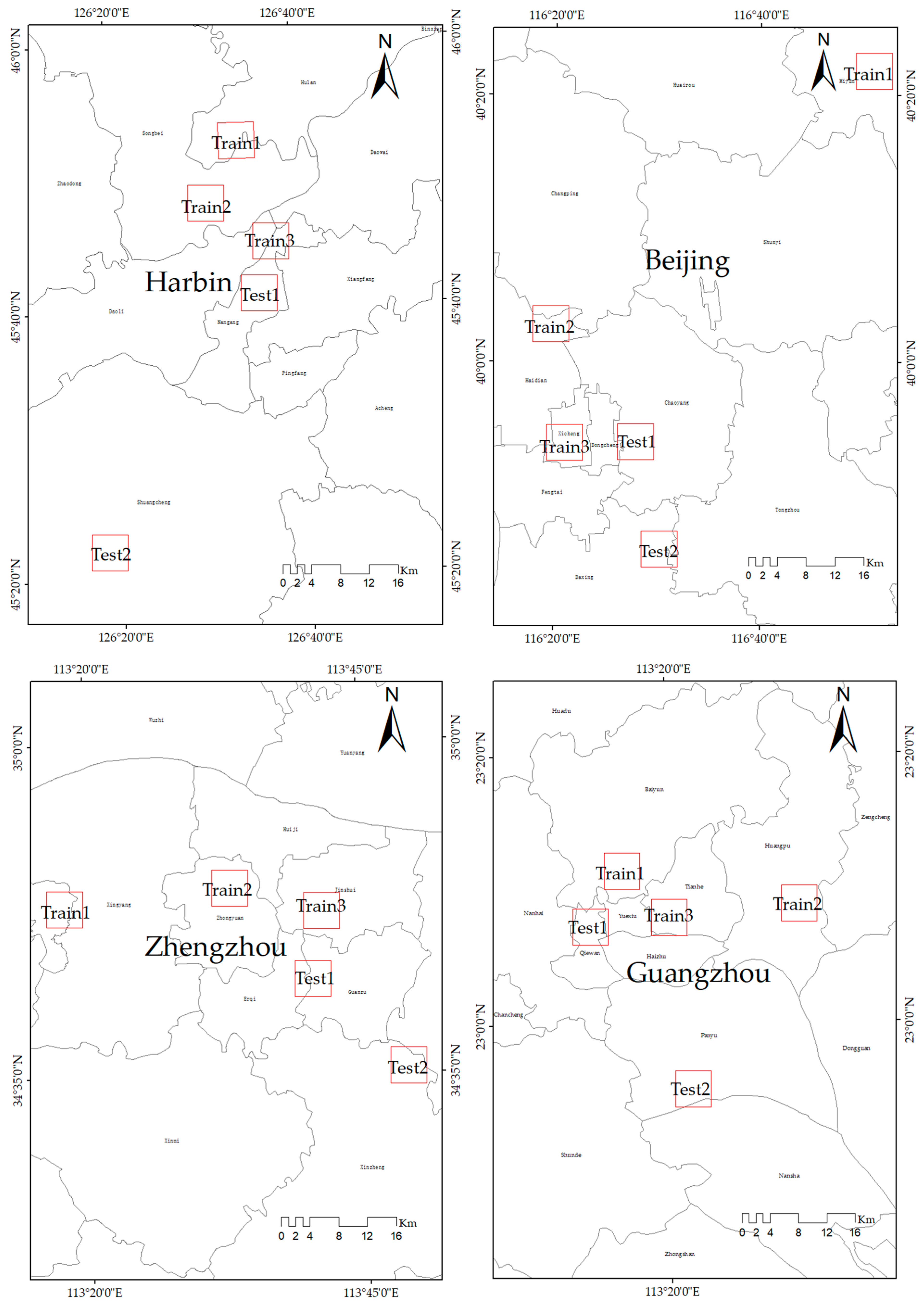
This paper extends previous work by studying the influence of seasonal and spatial factors on the effectiveness of FCN model in HRBs detection. More specifically, we study the performance of FCN model on Sentinel-2 data in different seasons and regions, also we want to evaluate the possibility to build one or a few FCN models rather than many local FCN models to handle the large diversity of HRBs in different regions and seasons without sacrificing much overall accuracy. To achieve this aim, we selected four cities, namely, Harbin, Beijing, Zhengzhou, and Guangzhou, as study regions. Four cities have diverse latitudes and landscapes. Additionally, we collected Sentinel-2 images from four seasons in each city. With multiple spatial and seasonal data, we design and conduct extensive experiments to evaluate the FCN-based method. Our study aims to answer three questions.
(1)
What are the performances of models built on different combinations of region and season?
(2)
Is it possible to build an effective model for all four seasons in a specific region?
(3)
Is it possible to build an effective model for all four regions and four seasons?
The paper is divided into five parts. Part one gives an introduction to our work. Part two describes the experimental data including images and HRBs samples, the flowchart of our method. Part three presents HRBs detection results and the analysis. Part four gives a discussion on the results. The final part concludes the paper and also provides perspectives in future work.

2. Materials and Methods

2.1. Data

Four capital cities namely Harbin, Beijing, Zhengzhou, Guangzhou ranging from north to south in China were selected as study regions as illustrated in Figure 1. Four cities have experienced extensive urbanization processes in the past decades; meanwhile, they are diverse from each other on many aspects such as latitude, climate, and landscape. According to Köppen climate classification, Harbin and Beijing belong to the Dwa, while Zhengzhou and Guangzhou pertain to Cwa. Thus, the selected regions provide a very good testbed for the validation of the effectiveness of the FCN-based method on HRBs detection. Fives typical areas were chosen for HRB sample collection in each region. Both urban center and suburban areas are considered in the selection. Each area covers about 5 km × 5 km. Among the five areas, three are used to train the FCN-based model while the other two are used as independent validation data. All selected sample areas and their corresponding regions are shown in Figure 2.
A total of 16 Sentinel-2 images covering all regions and seasons were collected in our study as indicated in Table 1. The images were selected as close as to the middle of each season. All data were acquired under clear sky conditions in 2018 except the data in Guangzhou in summer which was obtained in Summer in 2019 due to lacking of data with clear sky in summer in 2018. All data were processed to surface reflectance using the Sen2Cor program. Only three bands with 10 m spatial resolution were used in the study. They are Blue, Green, and Red as shown in Table 2.
To prepare train and validation samples for the FCN-based method, a slice with a size of 500 × 500 pixels is clipped for each sample region from its corresponding Sentinel-2 image. Then HRBs mask of the slice for each sample region is manually extracted based on visual interpretation of the subset image, high spatial resolution satellite images from Google Earth, and street-side imageries from Baidu Map. In the HRB mask acquisition process, we assume HRBs do not change in the sample region during 2018, and this assumption is largely valid according to our manual interpretation. This assumption can improve the accuracy of manual interpretation as the temporal change of image features of HRBs can be exploited. Figure 2 illustrates true color images and their corresponding HRBs labels in test1 in four regions respectively. Each clipped slice and its mask are further divided into patches with the size of 128 × 128. There is an overlap of 96 pixels to avoid the boundary effect in the patch preparation. Totally 432 patches were obtained for each sample region in each season. Typical patches with outlined HRBs from four regions in four seasons are illustrated in Figure 3. It can be seen that image features of HRBs seasonally vary a lot mainly due to changing shadows caused by the change of sun geometry while the spatial pattern of HRBs among seasons in the image keeps well in general.

2.2. Methodology

This paper aims to study the influence of seasonal and spatial factors on the effectiveness of the newly proposed FCN model in HRBs detection. More specifically, we want to answer the three questions posed in the introduction. For this purpose, we designed three groups of experiments by using the train and validation samples and the FCN model. In the following, the FCN model and its usage in the HRBs detection are firstly presented, and then the three groups of experiments are described in detail.
The architecture of the FCN model is illustrated in Figure 4. It can be generally seen as a combination of an encoder and a decoder. The encoder accepts raw remote sensing image patches as the input, and sequentially transforms the input patches into small but informative features through a trained VGG-16 model [23]. The output of pool5 in the encoder works as the input to the decoder. The decoder mainly uses the upsampling to recover the label image of HRBs from the encoded features. The dimension of features in each decoded layer is equal to the number of classes (two in our case, HRBs and others). The upsampling in the decoder is a transposed convolution with a fixed filter defined by the bilinear interpolation. Two skip layers connecting layers of the same size in the encoder and the decoder as shown in Figure 4 are used to enhance the spatial detail of label recovery. As the final layer, the softmax function transforms the decoded features into probabilities of HRBs and others, and then argmax function selects the label with the highest probability for each pixel and obtains a pixel-wise map of the HRB’s mask.
In real applications, the FCN model working as a supervised model needs to be trained before being put into use for HRB detection. In the training process, key parameters in the model are optimized based on the prepared train data and Adam learning algorithm [24]. The train data include a group of image pairs, and each pair contains a raw image patch with a size of 128 × 128 and its corresponding HRB’s mask. The mask is manually extracted based on the ground truth. In the inference process, an input image is firstly clipped into patches. Each clipped image patch is separately processed into an image patch of HRBs labels by the trained FCN model. The HRBs patches are spatially aligned according to their original locations in the input image. Thus a binary image of HRBs with the same size as the input image is obtained in the final. Here, the patch size for inference can be much larger than the patch size used in the training, which is 128 × 128. This is because the FCN inference works in a parallel mode, and each location is only affected by its effective receptive field, which has a size of 32 × 32 pixels in our model. Additionally, we set 32 pixels as the step of the moving window in the patch clip to alleviate the side effects caused by the spatial alignment of the boundary in the final result.
Three groups of experiments specifically designed in our study are coded as E1, E2, and E3, respectively. E1 mainly works to evaluate the FCN-based method under different combinations of season and region. E2 tries to evaluate the possibility to build an effective FCN model that is invariant to the season. E3 aims to study the possibility to build an effective FCN model that is invariant to both the region and the season. We list the experiments in detail as follows.
(1)
E1 evaluates FCN models built on different combinations of region and season.
In this group, totally 16 experiments are included as shown in Table 3. Each FCN model is trained and validated independently on a specific combination of region and season. Thus, the results can help to understand the behavior of the FCN-based method under different combinations of spatial and seasonal conditions. Additionally, the results in E1 can work as benchmarks for those of E2 and E3.
(2)
E2 evaluates the possibility to build an effective FCN model for all seasons in a fixed region.
Four experiments are designed in this group as shown in Table 4. Here, training samples from all four seasons in a specific region are combined to support the build of a single FCN mode that is effective for all seasons. Results from E1 are also used in this group for comparison. The results can help understand the behavior of the FCN-based method under different temporal conditions.
(3)
E3 evaluates the possibility to build a single effective FCN model for all seasons and regions.
Only one experiment is included in this group as shown in Table 5. Here, training samples from all four seasons and four regions are combined to support the build of a single FCN mode that is effective for all seasons and regions. Results from E1 and E2 are also used in this group for comparison. The results can help to understand the behavior of the FCN-based method under seasonal and spatial conditions.
As our purpose is to evaluate the FCN-based method under various spatial and temporal conditions, we used the same empirical key parameters in FCN training for all experiments as listed in Table 6. This group of parameters has been proven robust and effective in our previous study [8,9].
We used the F1 score to assess the performance of each trained model in all experiments. The F1 score can take advantage of the precision and recall as indicated in Equation (1), where an F1 score reaches its best value at 1 and worst at 0. It is more objective than overall accuracy in our binary classification case.
F1 score = 2 × (precision × recall)/(precision + recall),
where precision is the number of correct positive pixels divided by the number of all positive pixels predicted by the method, and recall is the number of correct positive pixels divided by the number of all relevant pixels.
All experiments are conducted under Ubuntu 16.04.6 LTS with Intel Core i7-5930 NVIDIA GeForce GTX 1080 and Memory 128 GB. The FCN model is built upon TensorFlow 1.8 and Python.

3. Results and Analysis

Totally 21 FCN models from E1, E2, and E3 were trained and validated according to the experimental design. The results were analyzed quantitatively and qualitatively as illustrated in Figure 5, Figure 6, Figure 7, Figure 8, Figure 9, Figure 10. To support a quantitative analysis, F1 scores of all trained FCN models on test data in each region are calculated to help analyze results from E1, E2, and E3 as shown in Figure 5, Figure 7 and Figure 9. Meanwhile, to fulfill a qualitative analysis, predicted results on test1 data in each region along with their corresponding images and ground truth are shown in Figure 6, Figure 8, and 
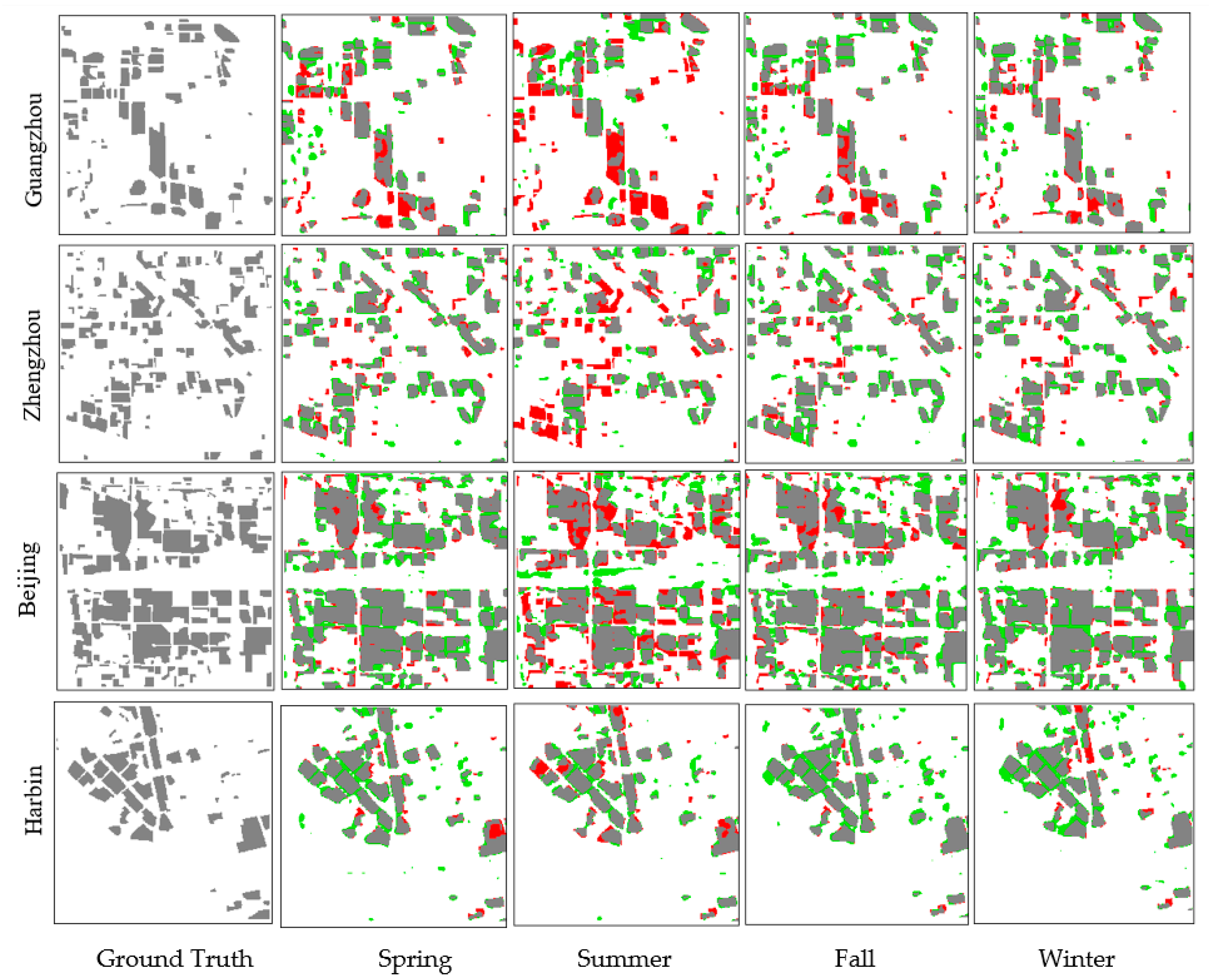
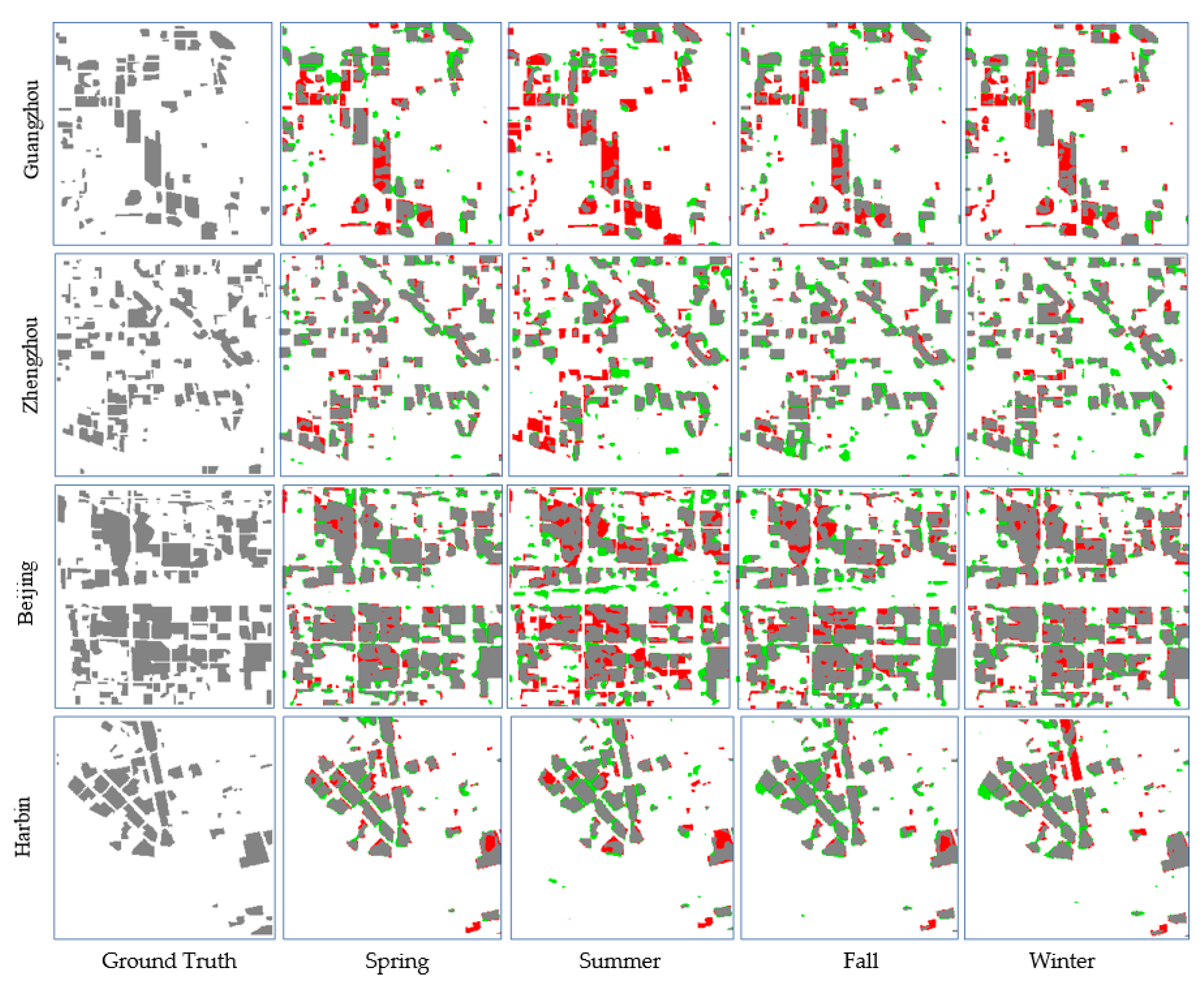
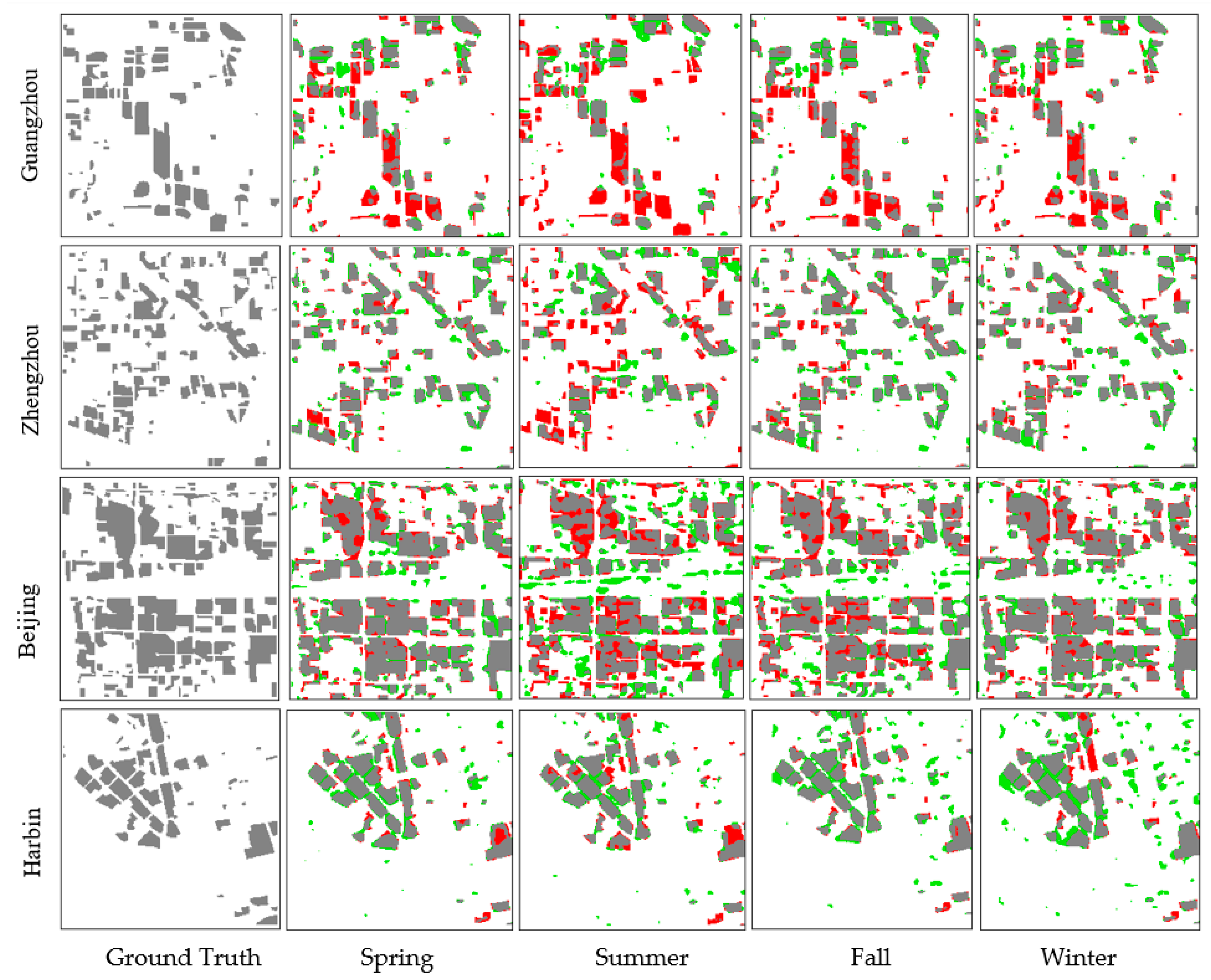
Figure 10 respectively. Also, for ease of visual interpretation of the Figures, true HRBs are colored in gray, omission errors are colored in red, and commission errors are colored in green. To answer three questions in our study, the results from E1, E2, and E3 are analyzed separately as follows.

3.1. Results and Analysis for E1

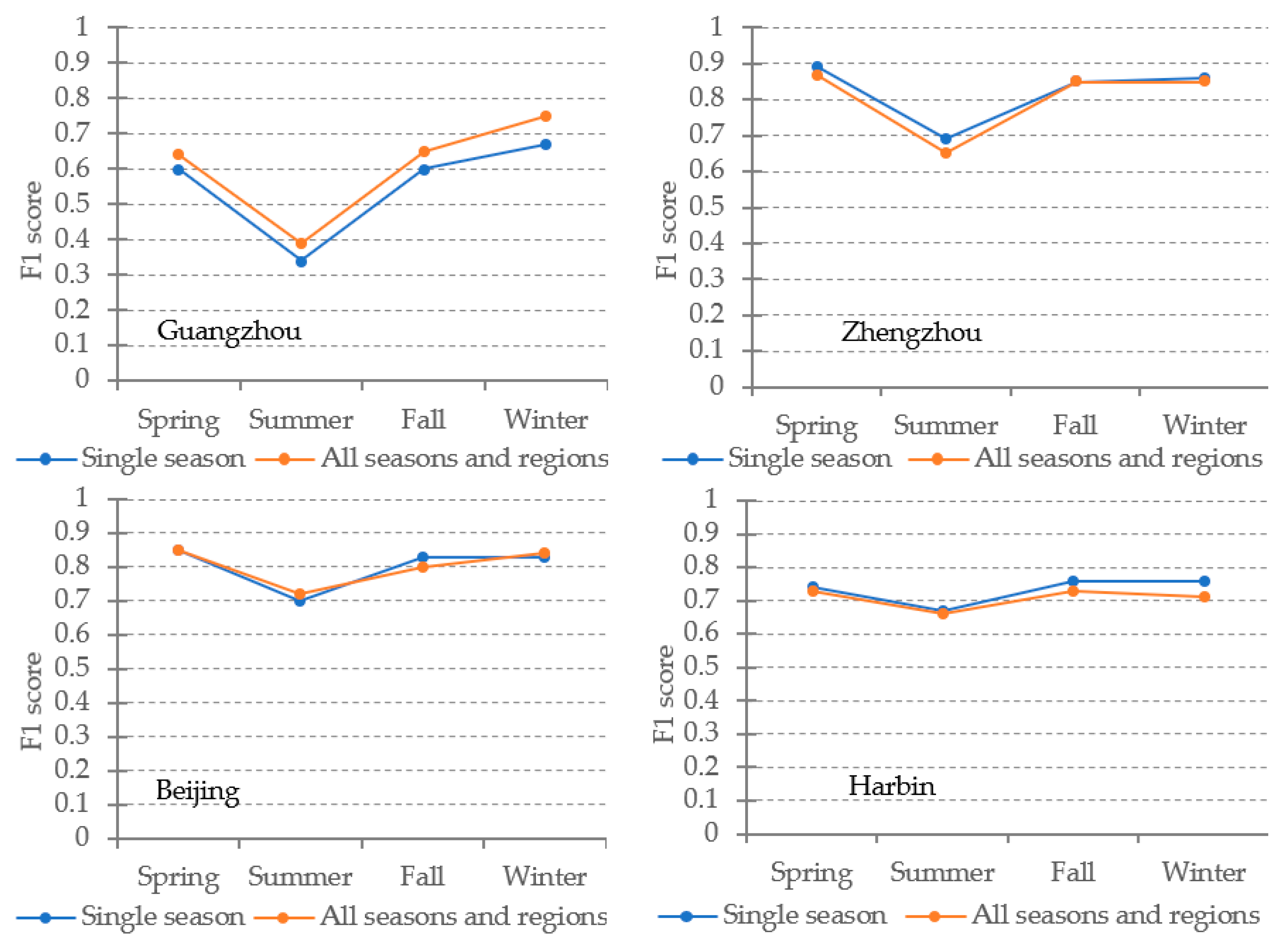
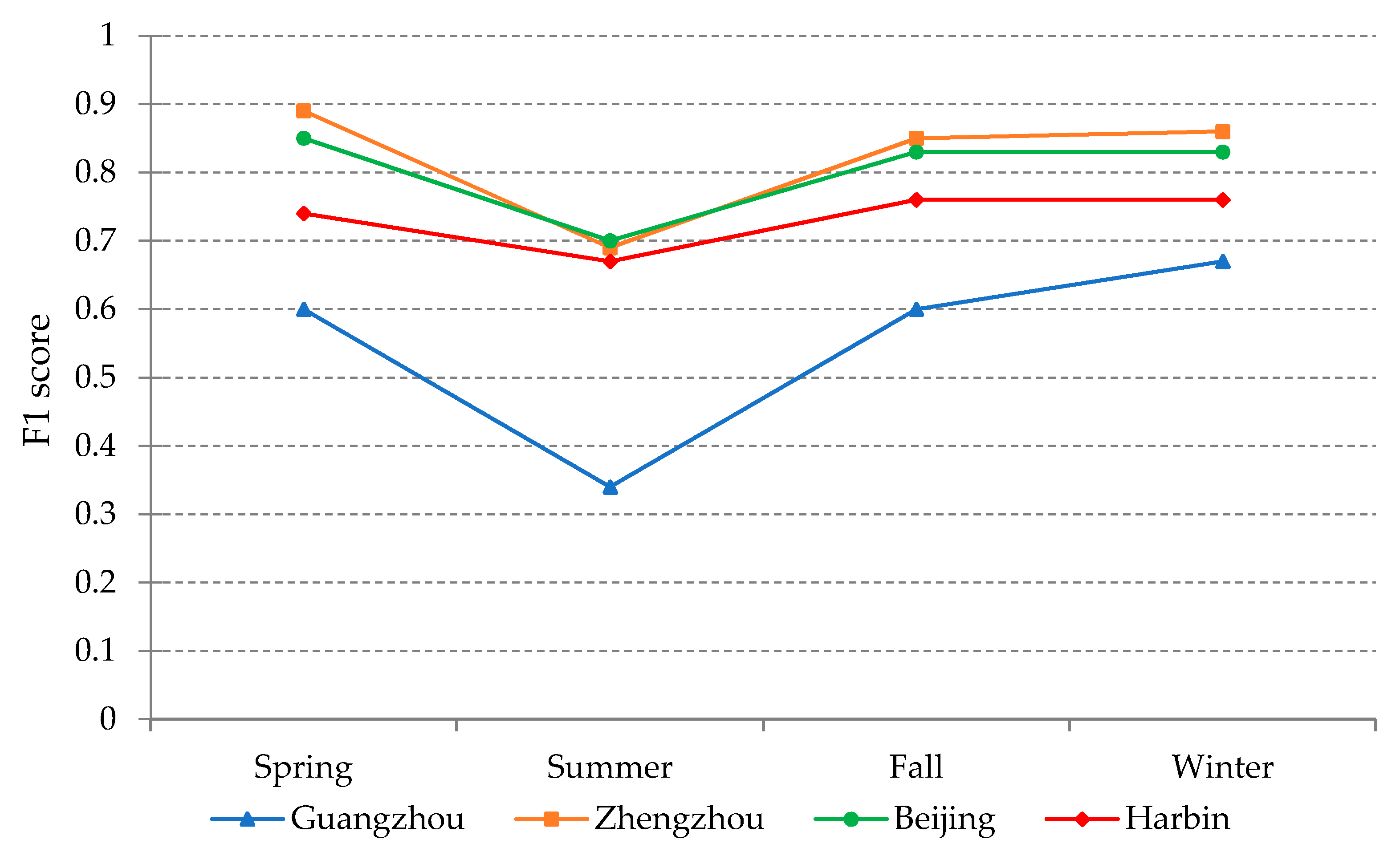
Figure 3 shows F1 scores of all trained FCN models on test data from 16 combinations of region and season. Figure 5 shows HRBs detection results of test1 data from four regions. Each result in E1 was predicted by the FCN model trained on data from the same combination of region and season as the validation.
As can be inferred from Figure 5, results from FCN models trained and validated on the same combination of season and region fluctuate among seasons and regions. The best result is about 0.90, which is obtained in Zhengzhou in Spring. The worst is about 0.35, which is obtained in Guangzhou in Summer. The accuracies of HRB detection results differ in four regions, more specifically, taking seasonally average accuracy of HRB detection results as the criteria, Guangzhou is about 0.55, and it is the worst compared to others. Zhengzhou is slightly better than Beijing, which is about 0.8, and both of them are better than Harbin, which is about 0.75. In terms of the season, the regional average accuracy of HRB detection results varies a little; however, the seasonal change of accuracy varies a lot among regions. The most distinct change is in summer, which is the worst for all regions. Among the regions, the results of Summer in Zhengzhou, Beijing, and Harbin are nearly the same at about 0.70, which is slightly worse than those of other seasons. While the result of summer in Guangzhou has an F1 score below 0.40, it has the largest decrease of accuracy compared to that of other seasons. If the season can be chosen to get a yearly best result, F1 score of detected HRBs can reach above 0.75 for all regions with most of the errors on the boundary of HRBs.
From Figure 6, we can see similar results to those in Figure 5 in terms of overall accuracy. Guangzhou has the lowest accuracy among the four regions. Summer has the lowest accuracy among the four seasons. However, the HRB detection results of test1 among seasons in each region are similar to the corresponding ground truth in the spatial distribution, and it is clear that the main differences among seasons lie on the boundary of detected HRBs in all regions. Furthermore, the accuracy of results in Guangzhou in summer does not look as worse as it is indicated in Figure 6 in terms of the location accuracy of HRBs.
The results from various combinations of region and season in E1 demonstrate the effectiveness of FCN-based method except at outlining the exact boundary. The shortage of the FCN model trained on a specific season in detecting the boundary of HRBs is mainly caused by dynamic image features in different seasons. The seasonal change of sun geometry makes the image features of HRBs change in a rather complex way, and this becomes distinct with the increase of the height. Nevertheless, by considering the seasonal change of image features, only one ground truth mask of HRBs is manually extracted for each region and it is the same for four seasons in the region. Thus, the discrepancy on boundaries between the predicted one and the ground truth is inevitable. Additionally, the bad performance of trained FCN model in summer, especially in Guangdong, is attributed to a near nadir sun geometry. Because a small solar zenith angle largely weakens the image feature of HRBs, this decreases the detection accuracy. However, the accuracy does not always increase with the solar zenith angle, as indicated by results from Harbin. Large solar zenith angle can enlarge shadows and cause them to overlap with other buildings and further increase the complexity of HRB detection.

3.2. Results and Analysis for E2

Figure 7 shows F1 scores of all trained FCN models on test data from 16 combinations of region and season. Also, results from E1 are included in Figure 7 for comparison. 
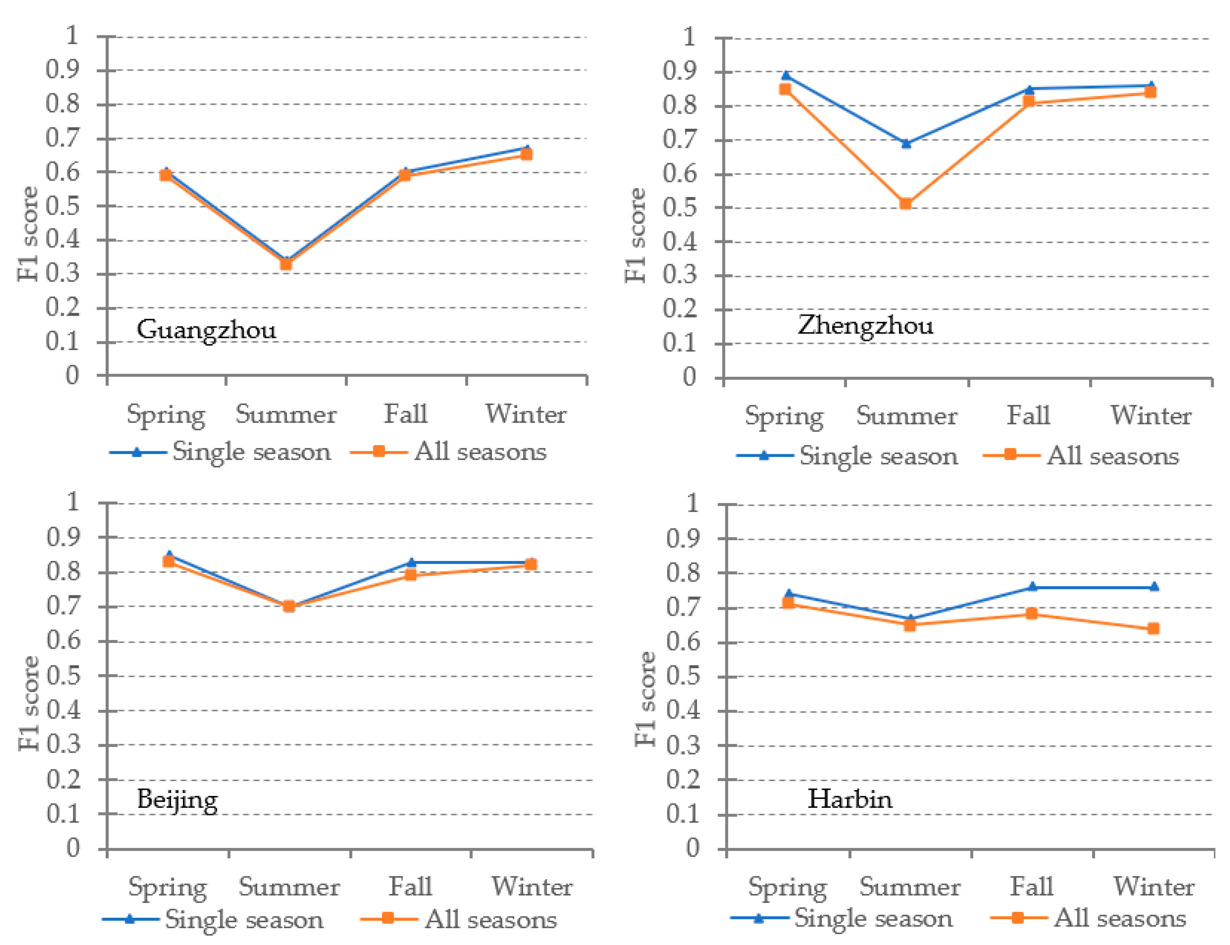
Figure 8 shows HRBs detection results of test1 data of four regions. Given a specific region, each result in E2 was predicted by the FCN model trained on seasonally combined samples from the same region as the validation data. Here, for convenience of read, we refer to the FCN model trained on samples from a specific combination of season and region as the single season model, and the FCN model trained on seasonally combined data from a specific region as the all seasons model.
As can be learned from Figure 7, single-season models are slightly better than their corresponding all-season models in terms of overall accuracy in most cases. The differences between single-season models and all-season models vary among four regions. More specifically, the differences in Guangzhou are tiny in all four seasons; results in Beijing follow the same trend in Guangzhou except a small amount of difference in fall; Zhengzhou has the most distinct difference at about 0.2 in summer, while differences are small in other seasons; the differences in fall and winter in Harbin are about 0.1. From Figure 6 and Figure 8, all-season models achieve similar results as single-season models. The results are similar to the ground truth in terms of spatial distribution. The uncertainties also lie on the boundary of detected HRBs in the results.
Results from E2 demonstrate the plausibility to replace four single-season models by a single all-season model in most of the regions in our study, although image features of HRBs seasonally change in a rather complex way due to the consistent change of sun geometry in a specific region. The advantage of the all-season model can be largely attributed to the powerful feature learning ability of FCN. However, as the mechanism of FCN is still in dark, it is hard to tell the shortage of the all-season model in some cases such as the Summer in Zhengzhou. Meanwhile, the boundary uncertainty in the HRBs detection results cannot be reduced through the combination of seasons. Similar reasons have been discussed in E1.

3.3. Results and Analysis for E3

Figure 9 shows F1 scores of all trained FCN models on test data from 16 combinations of region and season. Also, results from E1 are included for comparison. Figure 10 shows HRB detection results of test1 data of the four regions. The FCN model was trained on seasonally and regionally combined data. Here for convenience, we refer to the FCN model trained on seasonally and regionally combined data as the all-season and regions model.
As can be seen from Figure 9, single-season FCN models are close to all-seasons-and-regions models in terms of overall accuracy except the results in Guangzhou. The differences between the single season models and all seasons-and-regions models vary slightly among the four regions. More specifically, the accuracy of the all-seasons-and-regions model is consistently better than single-season models in Guangzhou, and the average difference is about 0.05. Single-season models perform slightly better than the corresponding all-seasons-and-regions models in Zhengzhou and Harbin, especially in spring and summer for Zhengzhou and in fall and winter in Harbin. In Beijing, the difference fluctuates at a small range in summer and fall. From Figure 6, Figure 8, and Figure 10, the all-seasons-and-regions models achieve similar results as the single-season model and the all-season model do. Both of the results are similar to the ground truth in terms of spatial distribution. The differences among the three group of results as indicated in Figure 9 cannot be easily observed through visual interpretation due to the spatial cluster property of the HRBs. Nevertheless, one thing in common is that the uncertainties of the results mostly lie on the boundary of detected HRBs.
Results from E3 demonstrate the plausibility to replace 16 single season and region models with a single all seasons and regions model in most of the cases in our study. Compared with results from the all seasons model in E2, the all-seasons-and-regions model is more accurate and stable at HRBs detection, no matter how image features of HRBs seasonally and regionally change. The advantage of the all-seasons-and-regions model is largely attributed to the powerful feature learning ability of the FCN model. Due to the black-box property of the FCN model as has been discussed in E2, similar seasons hold for the difficulty in explaining the shortage of the all-seasons-and-regions model in some cases such as in Guangzhou. Meanwhile, the boundary uncertainty in the HRB detection results cannot be reduced through the combination of seasons and regions in the training sample preparation.

4. Discussion

Our results show that the performance of the FCN-based method fluctuates among seasons and regions. The best F1 score can reach 0.9 in Zhengzhou in spring while the worst is below 0.4 in Guangzhou in summer. Compared to the large change of F1 scores, spatial patterns of the detected HRBs keep well for all seasons and regions, because most errors in the results locate on the boundary of HRBs. The value of the detected HRBs is high if the spatial pattern of HRBs is the key monitoring element. Furthermore, as a special type of land use, the HRBs monitoring frequency is usually longer than a year. In this sense, the newly proposed FCN-based method can achieve a yearly best F1 score of above 0.75 with most of the errors locating on the boundary of HRBs for regions with a large diversity in culture, latitude, and landscape. These results largely support the effectiveness of the method at the extraction of HRBs from Sentinel-2 data in large-scale regions if the best season can be chosen.
Our results also indicate that the use of data in summer in inference will lead to relatively poor results compared with data in other seasons. This may be mainly due to the fact that image features of HRBs are weakened by a small solar zenith angle in summer in the four selected regions. Thus, data in summer is not suggested for use in extracting HRBs if the timing is not as important as accuracy. One related problem of the FCN-based method is that it may be invalid in regions around the equator. In regions with very low latitude, the solar zenith angle is always small and even approaching zero, thus features of HRBs in the image will be nearly lost. The situation will be worse in underdeveloped regions where HRBs are sparsely located in urban areas, and also are relatively small compared to those in developed urban areas.
One unsolved problem in the study is the boundary effect of HRBs in the detection results. This is mainly due to the seasonal change of shadow of HRBs in both length and direction in urban areas caused by the change of sun geometry. Shadow works as an important component in the formation of image features of HRBs in our study. As HRBs are defined to be a spatial cluster, the change of shadows inside a cluster may not bring trouble to the HRBs detection given there are still enough image features left for learning. But shadows on the edge of the cluster can cause uncertainties in both training and inference stages for the FCN model. This is especially obvious when it comes to detect high and isolated buildings. One way to handle the problem may be by revising the definition of HRBs in a more rigorous way. The revised definition should be affected by shadows at a minimum level, independent of seasons and practical for HRB samples collection.

5. Conclusions

In this study, we designed three groups of experiments to empirically validate the ability of the newly proposed FCN-based method at HRB detection under various seasonal and spatial conditions. Results show that the FCN model trained on seasonally and regionally combined samples can achieve similar even better overall accuracy than that of the model trained on data from a specific combination of season and region. Our results support the potential to build a powerful FCN model on larger training samples for operational monitoring HRBs at the regional level even country scale.
One direction is to extend the FCN model on multi-temporal satellite data to track the changes of HRBs historically. The temporal HRBs at a large scale in a long time series will be very useful in many areas such as urban climate and urban planning, to name a few. However, since Sentinel-2 was put into operational work in 2016, we need to resort to other satellite data with a long history. The series of Landsat dating back to the 1980s can track urban development globally in the past 40 years [16]. One challenge is that the sensor setup is different between Landsat and Sentinel-2; more specifically, it is not clear whether the combination of the 15 m panchromatic data and the 30 m multispectral data in Landsat can provide enough image features as the Sentinel-2 data do in our study. Furthermore, the consistency of the detected HRB results in the time series, especially those lying on the boundary, needs to be handled in a proper way [15]. These are open questions to be studied in future work.

Author Contributions

B.Z. and L.L. had the original idea for the study. J.Z. and G.C. were responsible for data processing. L.L. conceived the experiments and carried out the analysis with assistance from J.Z.; L.L. structured and drafted the manuscript. All authors have read and agreed to the published version of the manuscript.

Funding

This research was funded by National Natural Science Foundation of China (grant number 41971327).

Data Availability Statement

Not applicable.

Acknowledgments

We thank Zhi Yan for his work on the FCN model development during his stay as a visiting graduate student in RADI, CAS. Also, L.L. thanks Wenzhi Liao from Ghent University, Belgium for the meaningful discussion on HRBs in early 2019 in Beijing. We also thank Denghui Fan in AIRCAS, CAS for his help in preparing the Figures in the revision.

Conflicts of Interest

The authors declare no conflict of interest.

References

  1. Kovačević, I.; Džidić, S. High-Rise Buildings–Structures and Materials; International BURCH University: Sarajevo, Bosnia and Herzegovina, 2018; pp. 17–22. [Google Scholar]
  2. Bechtel, B.; Alexander, P.J.; Böhner, J.; Ching, J.; Conrad, O.; Feddema, J.; Mills, G.; See, L.; Stewart, I. Mapping Local Climate Zones for a Worldwide Database of the Form and Function of Cities. ISPRS Int. J. Geo. Inf. 2015, 4, 199–219. [Google Scholar] [CrossRef] [Green Version]
  3. Stewart, I.D.; Oke, T.R. Local Climate Zones for Urban Temperature Studies. Bull. Am. Meteorol. Soc. 2012, 93, 1879–1900. [Google Scholar] [CrossRef]
  4. Mao, J.; Gao, N. The airborne transmission of infection between flats in high-rise residential buildings: A review. Build. Environ. 2015, 94, 516–531. [Google Scholar] [CrossRef]
  5. Miller, R.B.; Small, C. Cities from space: Potential applications of remote sensing in urban environmental research and policy. Environ. Sci. Policy 2003, 6, 129–137. [Google Scholar] [CrossRef]
  6. Esch, T.; Heldens, W.; Hirner, A.; Keil, M.; Marconcini, M.; Roth, A.; Zeidler, J.; Dech, S.; Strano, E. Breaking new ground in mapping human settlements from space – The Global Urban Footprint. ISPRS J. Photogramm. Remote Sens. 2017, 134, 30–42. [Google Scholar] [CrossRef] [Green Version]
  7. Taubenböck, H.; Esch, T.; Felbier, A.; Wiesner, M.; Roth, A.; Dech, S. Monitoring urbanization in mega cities from space. Remote Sens. Environ. 2012, 117, 162–176. [Google Scholar] [CrossRef]
  8. Song, X.-P.; Sexton, J.O.; Huang, C.; Channan, S.; Townshend, J.R. Characterizing the magnitude, timing and duration of urban growth from time series of Landsat-based estimates of impervious cover. Remote Sens. Environ. 2016, 175, 1–13. [Google Scholar] [CrossRef]
  9. Wang, L.; Li, C.; Ying, Q.; Cheng, X.; Wang, X.; Li, X.; Hu, L.; Liang, L.; Yu, L.; Huang, H.; et al. China’s urban expansion from 1990 to 2010 determined with satellite remote sensing. Chin. Sci. Bull. 2012, 57, 2802–2812. [Google Scholar] [CrossRef] [Green Version]
  10. Slonecker, E.T.; Jennings, D.B.; Garofalo, D. Remote sensing of impervious surfaces: A review. Remote Sens. Rev. 2001, 20, 227–255. [Google Scholar] [CrossRef]
  11. Gong, P.; Li, X.; Wang, J.; Bai, Y.; Chen, B.; Hu, T.; Liu, X.; Xu, B.; Yang, J.; Zhang, W.; et al. Annual maps of global artificial impervious area (GAIA) between 1985 and 2018. Remote Sens. Environ. 2020, 236, 111510. [Google Scholar] [CrossRef]
  12. Hu, S.; Wang, L. Automated urban land-use classification with remote sensing. Int. J. Remote Sens. 2012, 34, 790–803. [Google Scholar] [CrossRef]
  13. Huang, B.; Zhao, B.; Song, Y. Urban land-use mapping using a deep convolutional neural network with high spatial resolution multispectral remote sensing imagery. Remote Sens. Environ. 2018, 214, 73–86. [Google Scholar] [CrossRef]
  14. Yan, Z.; Li, L.W.; Cheng, G. Extraction of high-rise and low-rise building areas from Sentinel-2 data based on fully convolutional networks. Bull. Surv. Mapp. 2019, 7, 73–77. (In Chinese) [Google Scholar]
  15. Li, L.; Zhu, J.; Gao, L.; Cheng, G.; Zhang, B. Detecting and Analyzing the Increase of High-Rising Buildings to Monitor the Dynamic of the Xiong’an New Area. Sustainability 2020, 12, 4355. [Google Scholar] [CrossRef]
  16. Uniform Standard for Design of Civil Buildings GB 50252-2019. Available online: https://tujixiazai.com/biaozhunguifan/342889.html (accessed on 1 August 2021). (In Chinese).
  17. Li, J.; Roy, D.P. A Global Analysis of Sentinel-2A, Sentinel-2B and Landsat-8 Data Revisit Intervals and Implications for Terrestrial Monitoring. Remote Sens. 2017, 9, 902. [Google Scholar] [CrossRef] [Green Version]
  18. Zhang, L.; Zhang, L.; Du, B. Deep Learning for Remote Sensing Data: A Technical Tutorial on the State of the Art. IEEE Geosci. Remote Sens. Mag. 2016, 4, 22–40. [Google Scholar] [CrossRef]
  19. Zhu, X.X.; Tuia, D.; Mou, L.; Xia, G.-S.; Zhang, L.; Xu, F.; Fraundorfer, F. Deep Learning in Remote Sensing: A Comprehensive Review and List of Resources. IEEE Geosci. Remote Sens. Mag. 2017, 5, 8–36. [Google Scholar] [CrossRef] [Green Version]
  20. Shelhamer, E.; Long, J.; Darrell, T. Fully Convolutional Networks for Semantic Segmentation. IEEE Trans. Pattern Anal. Mach. Intell. 2016, 39, 640–651. [Google Scholar] [CrossRef]
  21. Badrinarayanan, V.; Badrinarayanan, V.; Cipolla, R. SegNet: A Deep Convolutional Encoder-Decoder Architecture for Image Segmentation. IEEE Trans. Pattern Anal. Mach. Intell. 2017, 39, 2481–2495. [Google Scholar] [CrossRef]
  22. Li, L.; Yan, Z.; Shen, Q.; Cheng, G.; Gao, L.; Zhang, B. Water Body Extraction from Very High Spatial Resolution Remote Sensing Data Based on Fully Convolutional Networks. Remote Sens. 2019, 11, 1162. [Google Scholar] [CrossRef] [Green Version]
  23. Simonyan, K.; Zisserman, A. Very deep convolutional networks for large-scale image recognition. arXiv 2014, arXiv:1409.1556. [Google Scholar]
  24. Kingma, D.; Ba, J. Adam: A Method for Stochastic Optimization. arXiv 2014, arXiv:1412.6980. [Google Scholar]
Figure 1. Illustrations of five regions selected in our study and five sample areas in each region used for sample collection (Red boxes show the selected sample areas).
Remotesensing 13 04073 g001
Figure 2. True color images in Spring and the corresponding HRBs masks in test1 in Guangzhou, Zhengzhou, Beijing, and Harbin from top to bottom, respectively.
Remotesensing 13 04073 g002
Figure 3. True-color images of patches selected from four cities and four seasons, and red rectangles refer to HRBs in the patches.
Remotesensing 13 04073 g003
Figure 4. The architecture of the FCN model used in our experiments. The white boxes indicate image features with their sizes shown in the box. Color bars represent modules with specific functions as explained at the lower-left corner.
Remotesensing 13 04073 g004
Figure 5. F1 scores of FCN models validated on different combinations of region and season. Each model is trained on the same combination as that of the validation.
Remotesensing 13 04073 g005
Figure 6. Ground truths and predicted HRBs in test1 in four regions in four seasons by FCN models trained on samples from each combination of season and region. Gray refers to true HRBs, red refer to omission errors, and green refer to commission errors.
Remotesensing 13 04073 g006
Figure 7. F1 scores of FCN models validated on different combinations of region and season. Single season model in blue line is trained on samples in a specific combination of season and region. All-season model in yellow line is trained on the seasonally combined samples in a specific region.
Remotesensing 13 04073 g007
Figure 8. Ground truths and predicted HRBs in test1 in four regions in four seasons by FCN models trained on seasonally combined samples. Gray refers to true HRBs, red refer to omission errors, and green refer to commission errors.
Remotesensing 13 04073 g008
Figure 9. F1 scores of FCN models validated on different combinations of region and season. All seasons and regions model in yellow line is trained on the seasonally and regionally combined samples.
Remotesensing 13 04073 g009
Figure 10. Ground truths and predicted HRBs in test1 in four regions in four seasons by FCN models trained on seasonally and regionally combined samples. Gray refers to true HRBs, red refer to omission errors, and green refer to commission errors.
Remotesensing 13 04073 g010
Table 1. List of dates and locations of Sentinel-2 images used in the experiment.
Tile (City)T51TYL
(Harbin)
T50TMK
(Beijing)
T49SGU
(Zhengzhou)
T49QGF
(Guangzhou)
Season
Spring22 March 201812 February 201822 February 201811 March 2018
Summer23 June 201814 June 201807 June 201814 June 2019
Fall18 September 201805 September 201830 September 201802 October 2018
Winter10 December 201819 December 201829 December 201815 January 2018
Table 2. Spectral and spatial configurations of Sentinel-2 data used in the experiment.
Band IndexNameWavelength (nm)Spatial Resolution
2Blue458–52310 m
3Green543–57810 m
4Red650–68010 m
Table 3. Experimental setup for E1.
No.RegionSeasonModel
1GuangzhouSpringFCN
2GuangzhouSummerFCN
3GuangzhouFallFCN
4GuangzhouWinterFCN
5ZhengzhouSpringFCN
6ZhengzhouSummerFCN
7ZhengzhouFallFCN
8ZhengzhouWinterFCN
9BeijingSpringFCN
10BeijingSummerFCN
11BeijingFallFCN
12BeijingWinterFCN
13HarbinSpringFCN
14HarbinSummerFCN
15HarbinFallFCN
16HarbinWinterFCN
Table 4. Experimental setup for E2.
No. RegionSeasonModel
1GuangzhouSpring + Summer + Fall + WinterFCN
2ZhengzhouSpring + Summer + Fall + WinterFCN
3BeijingSpring + Summer + Fall + WinterFCN
4HarbinSpring + Summer + Fall + WinterFCN
Table 5. Experimental setup for E3.
No.RegionSeasonModel
1Guangzhou + Zhengzhou + Beijing + HarbinSpring + Summer + Fall + WinterFCN
Table 6. Key parameters in the FCN model training.
ParametersValueExplanations
Input featureRGBRed, Green and Blue
transfer learningYesReusing trained weights of VGG-16 on ImageNet
InitializerXavierInitialize the weight of the network before training
batch size1The number of patch used in each round of training
patch size128The size of input patch
training step60,000We output a trained model at each 3000 steps and select the one with the best performance on the training data
loss functionCross-entropyMeasurement of loss in the optimization
optimizer AdamAlgorithm for updating the weight [24]
learning rate0.00001Key parameter in the Adam
Publisher’s Note: MDPI stays neutral with regard to jurisdictional claims in published maps and institutional affiliations.

