Hyperspectral Image Super-Resolution Based on Spatial Correlation-Regularized Unmixing Convolutional Neural Network

Abstract

Super-resolution (SR) technology has emerged as an effective tool for image analysis and interpretation. However, single hyperspectral (HS) image SR remains challenging, due to the high spectral dimensionality and lack of available high-resolution information of auxiliary sources. To fully exploit the spectral and spatial characteristics, in this paper, a novel single HS image SR approach is proposed based on a spatial correlation-regularized unmixing convolutional neural network (CNN). The proposed approach takes advantage of a CNN to explore the collaborative spatial and spectral information of an HS image and infer the high-resolution abundance maps, thereby reconstructing the anticipated high-resolution HS image via the linear spectral mixture model. Moreover, a dual-branch architecture network and spatial spread transform function are employed to characterize the spatial correlation between the high- and low-resolution HS images, aiming at promoting the fidelity of the super-resolved image. Experiments on three public remote sensing HS images demonstrate the feasibility and superiority in terms of spectral fidelity, compared with some state-of-the-art HS image super-resolution methods.

1. Introduction

Hyperspectral (HS) remote sensing images always suffer from the deficiency of low spatial resolution and mixed pixels, which seriously deteriorate the performance of target detection and recognition in Earth observation areas. Therefore, the demand for potential spatial resolution enhancement has generated considerable interest in the area of remote sensing. Currently, HS image super-resolution (SR) techniques can be divided into two categories, namely single image super-resolution and image fusion techniques. In practice, the fusion of an HS image with a higher-resolution panchromatic (PAN) or multispectral (MS) image is the prevailing technology, which has been extensively studied since the beginning of this century. This technology is also known as hyper-sharpening in the area of remote sensing image processing [1]. Thus far, numerous hyper-sharpening approaches have been investigated that can be roughly summarized into the following categories: (1) extensions of MS pan-sharpening approaches [2,3], (2) Bayesian-based approaches [4,5], (3) matrix factorization or tensor-based approaches [6,7,8,9], (4) deep learning (DL)-based approaches [10,11,12,13], and (5) others [14,15,16]. Detailed analyses of HS image fusion techniques can be found in [17,18,19].

In general, hyper-sharpening techniques require an auxiliary higher-resolution co-registered image, which is not always available in practical applications. For this reason, most current studies utilize synthetic data sets to demonstrate the effectiveness of their approaches, which means that the higher-resolution PAN or MS image is commonly synthesized by band averaging of the HS image. In such situations, only a few studies have taken account of the effects of different platforms or acquisition conditions [20,21]. Therefore, this is a major obstacle in the hyper-sharpening field.

On the contrary, the single image super-resolution technique [22,23] has the ability to convert a low-resolution (LR) HS image into a high-resolution (HR) one without supplementary sources, which has also become a fascinating topic in related areas. Single image SR techniques aim at exploiting the abundant spectral correlations among the spectral bands of the HS images and predicting the spatial distribution of pixels under higher resolutions. Perhaps one of the earliest HS SR approaches was the linear deterministic model of the HS image acquisition process proposed in [24]. Although the reconstruction process seems to be relatively rough nowadays, it still has great theoretical significance in the HS SR field. Motivated by this attempt, a number of SR approaches have been proposed for HS images based on either conventional or, in later years, on deep learning-based techniques. Patel et al. [25] presented a wavelet transform-based SR method, where the novelty lies in designing an application-specific wavelet basis. Considering the inherent sparse property of HS images, sparse representation also became a popular approach to model the SR problem. Li et al. [26] proposed an HS SR framework utilizing spectral mixture analysis and spatial–spectral group sparsity by simultaneously combining the sparsity and the nonlocal self-similarity of the images in the spatial and spectral domains, thus providing excellent spectral consistency performance. Dong et al. [27] proposed an HS SR method by formulating the estimation of an HS image as a joint estimation of dictionary and sparse codes based on the prior knowledge of the spatial–spectral sparsity of the HS image. Furthermore, Irmak et al. [28] proposed a Bayesian super-resolution algorithm that converts the SR reconstruction problem in the spectral domain to a quadratic optimization problem in the abundance map domain and yields high quality in preserving the spectral consistency.

During the past five years, with the rapid development of deep learning techniques, convolutional neural networks (CNNs) have been extensively researched and applied in a range of image-related works [29]. Naturally, a series of image SR methods based on CNN have been proposed successively. For instance, the Laplacian Pyramid Super-Resolution Network (LapSRN) was proposed in [30,31] to predict the sub-band residuals in a coarse-to-fine fashion. It outperforms a number of state-of-the-art methods in terms of speed and accuracy. The main deficiency of LapSRN is the increment of network depth regarding different upsampling scale factors and the limitation of upsampling scales for training.

In particular, for HS images, Hu et al. [32] presented a deep spectral difference CNN (SDCNN) with the combination of a spatial-error correction model, which automatically selects and super-resolves the key band, and learns the spectral difference mapping between LR and HR images. In [33], a 3D full CNN architecture was designed to directly learn an end-to-end mapping between low-spatial-resolution and high-spatial-resolution HS images. It also designs a sensor-specific mode to adapt to a different scene but acquired by the same sensor. The experiments demonstrate its higher quality both in reconstruction and spectral fidelity. Arun and Hu et al. [34,35] also proposed two additional 3D CNN-based SR methods. Arun et al. [34] utilized a convolution–deconvolution framework and hypercube-specific loss functions. Moreover, the spatial–spectral accuracy of the super-resolved hypercubes, in terms of the validity of regularizing features and endmembers, was explored to devise an optimal ensemble strategy. Hu et al. [35] utilized a multiscale feature fusion and aggregation network with 3D convolution, and proposed a spectral gradient loss function to prevent spectral distortion. Inspired by the unmixing idea of [6], a deep feature matrix factorization (DFMF)-based SR method was proposed in [36], by incorporating a CNN and nonnegative matrix factorization strategy. Zou et al. [37] presented a deep residual CNN and spectral unmixing-based SR method, which shows good performance in preserving the spatial and spectral information of HS images. Li et al. [38] placed the SR process in a generative adversarial network (GAN), and incorporated the band attention mechanism into the network to explore the correlation of spectral bands and avoid spectral distortion. Hu et al. [39] presented an intrafusion network for HS image SR, which consists of a spectral difference module, parallel convolution module, and intrafusion module [40]. These three modules show generalization capacity and effectiveness on both CNN and residual networks. Jiang et al. [41] focused on the adaptation of a deep learning-based single gray/RGB image SR method for HS images, and introduced a spatial–spectral prior network (SSPN). To tackle the small sample problem, SSPN proposes a group convolution and progressive upsampling framework. Experiments demonstrate its superiority in enhancing the spatial details of the recovered image. Based on the recurrent neural network (RNN), Fu et al. [42] proposed a bidirectional 3D quasi-RNN that combines both CNN and RNN for single HS SR work, and they achieved improvements in terms of both restoration accuracy and visual quality. Shi et al. proposed super-resolution approaches by incorporating attention modules [43] and a generative adversarial network [44,45], which achieves better visual quality over some state-of-the-art approaches. A brief analysis and comparison of recent HS image SR methods can be found in [46].

Generally, HS images with high and low resolutions reflect the spectral characteristics of the same ground objects from different scales. Hence, some instinctive property remains invariable. From the perspective of the spectrum mixture, it is characterized by the spectral endmembers. Naturally, taking account of the spectral mixture model is definitely beneficial to preserve the overall spectral characteristics for single HS image super-resolution tasks. Unfortunately, only a few efforts have been made so far. Recently, we proposed an HS and MS image fusion method based on CNN and spectral unmixing models [47], which fully exploits the characteristics of high spectral and spatial resolution of HS and MS images, respectively, and aims to better estimate the abundances for HR HS images. The fusion method achieves state-of-the-art performance in terms of spectral fidelity. Nevertheless, this method still needs MS images to provide auxiliary HR spatial information. To overcome this deficiency, inspired by the existing single HS SR methods [26,36] and the unmixing-based fusion method [47], in this paper, a CNN-based single image super-resolution approach is proposed, via the classical linear spectral mixture model, to spatially improve the resolution of HS images without auxiliary image sources. The proposed approach, named the unmixing CNN (UCNN) SR approach, assumes that the differences between high- and low-resolution HS images concentrate on the abundances of endmembers for the same scene, thereby employing a CNN to solve the HR abundance maps. Furthermore, since the LR HS image is the degraded version of HR HS image, the spatial correlation between the HR and LR image can be formulated by the spatial spread transform matrix. Therefore, we propose a spatial correlation-regularized CNN to refine the prediction of abundance maps. The main contributions of this work are summarized as follows.

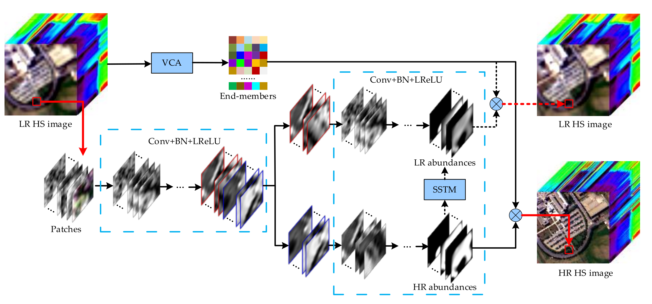
• A CNN-based single HS image SR framework is proposed, which incorporates the linear spectral mixture model to fully exploit the intrinsic properties of HS images, thereby improving the spatial resolution of HS images, without auxiliary sources.
• The correlation between the high- and low-resolution HS images is characterized by the spatial spread transform function, which helps to preserve the spectra of the super-resolved image.
• A loss function regarding the spectral mixture models and spatial correlation regularization is defined to effectively train the proposed network.

Experiments on several public HS images demonstrate the effectiveness and performance of the proposed approach. The remainder of this paper is organized as follows. Section 2 elaborates the proposed CNN-based SR method. Section 3 describes the experiments and results. Finally, the conclusions are drawn in Section 4.

2. Methodology

2.1. Observation Models

Suppose that the desired high-resolution HS image is denoted by $Y\in {ℝ}^{\mathsf{\Lambda }\times N}$, where $\mathsf{\Lambda }$ is the number of spectral bands, and $N$ denotes the pixel number. According to the linear spectral mixture model [47], we have

$$Y=E_Y{A}_Y+N_Y,$$

(1)

where $E_Y\in {ℝ}^{\mathsf{\Lambda }\times D}$ and $A_Y\in {ℝ}^{D\times N}$ are the spectral endmember matrix and abundance matrix, respectively. $D$ is the number of endmembers, which can be determined by either empirical criteria [6,7] or endmember estimation methods, e.g., thresholding ridge ratio criterion [48], agglomerative clustering [49], saliency-based autonomous endmember detection [50], etc. $N_Y\in {ℝ}^{\mathsf{\Lambda }\times N}$ is the residual. Correspondingly, the observable low-resolution HS image is denoted by $X\in {ℝ}^{\mathsf{\Lambda }\times n}$, where n denotes the pixel number of the LR HS image. $r=\sqrt{N/n}$ stands for the resolution ratio. In many cases, the LR HS image will be upscaled to the size of the HR HS image, via a bilinear or bicubic interpolation method. In other words, $X$ has the same pixel number as $Y$, namely $X\in {ℝ}^{\mathsf{\Lambda }\times N}$, and we have

$$X=E_X{A}_X+N_X.$$

(2)

$E_X\in {ℝ}^{\mathsf{\Lambda }\times D}$, $A_X\in {ℝ}^{D\times N}$ and $N_X\in {ℝ}^{\mathsf{\Lambda }\times N}$ are defined similarly as aforementioned, but at lower resolution. In general, we have $E_Y=E_X=E$, which reflects the overall spectral attributes of ground objects for the same scene. Accordingly, the abundance matrices $A_X$ and $A_Y$ describe the spatial distribution of ground objects at different resolutions. Suppose that $S\in {ℝ}^{N\times N}$ denotes the spatial spread transform matrix (SSTM) [6,10] that is used to formulate the transformation between each pixel of $X$ and the corresponding pixel, with its neighbors, of $Y$. For instance, a Gaussian low-pass filter [6] can be used to simulate the degradation of resolution and applied to each pixel with its neighbors for the HR image. Then, each column of SSTM is the vectorization of the Gaussian filter at proper locations. In other words, $S$ represents the spatial degradation function between the high-resolution image and its counterpart for each pixel. Consequently, we have $X=YS$, and obviously, we also have

$$E_Y{A}_{Y}S=E_X{A}_X.$$

(3)

Therefore, the LR abundance matrix is given by

$$A_X=A_{Y}S.$$

(4)

The spatial spread transform matrix $S$ is a sparse matrix, as well as the abundance matrices $A_X$ and $A_Y$. Moreover, (4) suggests that the spatial correlation between LR and HR HS images can also be characterized by the spatial spread transform function between the LR and HR abundances. Therefore, in this paper, an HS image SR approach is proposed, which employs a CNN to resolve the high-resolution abundance matrix, thereby reconstructing the anticipated HR HS image.

2.2. HS Image Super-Resolution via UCNN

The main framework of our proposed UCNN SR approach is shown in Figure 1. First, the primal HS image is upsampled by the factor $r$ using a bicubic interpolation method, to keep the same size as the HR HS image. Then, the initial endmembers are extracted by vertex component analysis (VCA), which is a widely used endmember extraction method [6,36], from the HS image. Instead of feeding the entire HS image into the network, small pieces of patches are obtained by partitioning the HS image into sub-images of $p\times p$ size, in a pixel-by-pixel manner [33,39,41].

The architecture of our proposed network is composed of a series of convolutional layers, which can be imitatively divided into two stages, feature extraction and abundance prediction. The first stage consists of 6 convolutional layers, with each followed by a batch normalization (BN) layer and a leaky rectified linear unit (ReLU) function with $\alpha =0.2$, successively. Each convolutional layer involves C_out filters, resulting in C_out intermediate feature maps. Afterwards, the last C_out feature maps are split into two groups (the maps with red and blue boundaries in Figure 1) and fed into a two-branch prediction stage. In our preliminary works for this paper, we found that the number of C_out actually has a limited influence on the super-resolution results. According to the existing works, a typical number of 64 is used in the experimental section. The 64 feature maps are then split into two groups, with each group containing C_out/2 = 32 maps that are fed into the two branches, respectively. Here, we suggest a bisection of feature maps, since, in this manner, the upper branch and lower branch have the same time and space complexities, which simplifies the development of implementation programs.

Both branches employ 4 convolutional layers to predict the LR and HR abundance maps individually. The first 3 convolutional layers of each branch contain 64 filters, and are also followed by the BN and leaky ReLU layers, individually, whereas the last layer contains D filters, corresponding to the D abundance maps. Here, D is the preset endmember numbers. Finally, an output layer with the Softmax function is appended to constrain the nonnegativity and sum-to-one property of abundances. Thus, the desired HR HS image is obtained by multiplying the endmembers, and the HR abundance matrix that is acquired by the lower branch, according to (1). Likewise, the LR HS image can also be reconstructed by multiplying the endmembers and LR abundance matrix acquired by the upper branch in Figure 1.

Moreover, in this proposed network, the sizes of convolutional filters are commonly set to 3 × 3, and the mirror padding mode is applied to preserve the original size of the patches. The network can be easily trained by adaptive moment estimation (ADAM) with the back-propagation method [32,51]. Suppose that the training sample patches are also represented by the aforementioned symbols, e.g., $X$, $Y$, $A$, etc., for convenience. Let ${\tilde{A}}_X$ and ${\tilde{A}}_Y$ be the predicted LR and HR abundance matrices, respectively. Considering (1) and (2), the aim of each branch is to minimize the prediction errors as follows:

$$\begin{array}{c}min{L}_1=\underset{{\tilde{A}}_X}{min}||X-E{\tilde{A}}_X{||}_{\mathrm{F}}^2, s.t.||{\tilde{A}}_X{||}_0\le \epsilon ,\\ min{L}_2=\underset{{\tilde{A}}_Y}{min}||Y-E{\tilde{A}}_Y{||}_{\mathrm{F}}^2, s.t.||{\tilde{A}}_Y{||}_0\le \epsilon ,\end{array}$$

(5)

where $|| {||}_{\mathrm{F}}$ and $|| {||}_0$ are the Frobenius and L0 norms, respectively. $\epsilon$ is used to control the sparsity of abundances $E=E_Y=E_X$.

As shown in Figure 1, the correlation between the LR and HR abundance maps can be described by (4). Therefore, a spatial correlation-regularized loss function is defined for the entire network as follows:

$$\begin{array}{ll}L& =\frac{1}{2}||X-E{\tilde{A}}_X{||}_F^2+\frac{1}{2}||Y-E{\tilde{A}}_Y{||}_F^2\\ & +\frac{1}{2}||{\tilde{A}}_X-{\tilde{A}}_{Y}S{||}_F^2+\eta \cdot \frac{1}{2}\left(||{\tilde{A}}_X{||}_2^2+||{\tilde{A}}_Y{||}_2^2\right),\end{array}$$

(6)

in which $\eta$ is the balance parameter that controls the approximation and the sparsity of abundances. In this work, we use $|| {||}_2$ instead of $|| {||}_0$ to promote the generalization ability of the network [44,52]. Note that the SSTM defined in (6) $S\in {ℝ}^{p^2\times p^2}$ is actually a local transform matrix with $p^2\times p^2$ elements, which transforms each pixel from the HR image patch to the LR patch, rather than the global transform matrix in (3). In this paper, we employ a Gaussian low-pass filter with (2r − 1) × (2r − 1) elements to simulate the transformation between HR and LR pixels. Then, each column of $S$ corresponds to the vectorized filter at proper locations. Afterwards, the derivatives of the loss function with respect to the output abundances of two branches, ${\tilde{A}}_X$ and ${\tilde{A}}_Y$, can be computed by

$$\begin{array}{l}\frac{dL}{d{\tilde{A}}_X}=E^{\mathrm{T}}\left(E{\tilde{A}}_X-X\right)+\left({\tilde{A}}_X-{\tilde{A}}_{Y}S\right)+\eta {\tilde{A}}_X\\ \frac{dL}{d{\tilde{A}}_Y}=E^{\mathrm{T}}\left(E{\tilde{A}}_Y-Y\right)+\left({\tilde{A}}_{Y}S-{\tilde{A}}_X\right)S^{\mathrm{T}}+\eta {\tilde{A}}_Y.\end{array}$$

(7)

Moreover, the derivates of network weights can be calculated accordingly. In addition, we also prefer to fine-tune the endmember matrix during the network training phase by using the multiplicative update rule to ensure that it can converge to local optima under the nonnegativity constraints:

$$E\leftarrow E.\times \frac{X{\tilde{A}}_X^{\mathrm{T}}+Y{\tilde{A}}_Y^{\mathrm{T}}}{E{\tilde{A}}_X{\tilde{A}}_X^{\mathrm{T}}+E{\tilde{A}}_Y{\tilde{A}}_Y^{\mathrm{T}}}$$

(8)

where $.\times$ and $./$ denote the elementwise multiplication and division, respectively. Thus, $E$ will be updated during each epoch of the network training until a maximum epoch number is met. It should be also pointed out that the LR abundance prediction branch will only be implemented during the training stage. Once the network is trained, only the HR abundances are required to eventually obtain the HR HS image.

3. Experimental Data Sets and Results

3.1. Experimental Setup

In order to demonstrate the effectiveness and superiority of our proposed approach, the following widely used HS data sets were utilized to conduct super-resolution experiments.

The first HS image was collected by the Reflective Optics System Imaging Spectrometer (ROSIS) over the University of Pavia, Italy. It consists of $610\times 340$ pixels and 103 spectral bands, with a spatial resolution of approximately 1.3 m. The second image was collected by the compact airborne spectrographic imager sensor (CASI) with a spatial resolution of 2.5 m, over the University of Houston, USA. There are $1905\times 349$ pixels and 144 spectral bands, with a pixel resolution of 2.5 m. The last image is a low-altitude Airborne Visible Infrared Imaging Spectrometer (AVIRIS) image collected over the North Island of the U.S. Naval Air Station in San Diego, CA, USA. It has $400\times 400$ pixels and 189 bands with a spatial resolution of 3.5 m, after removing noisy bands. Two subsets of each image were selected as the training and testing areas for our experiments, which are shown in Figure 2. The training and testing sub-images in this paper have the same spatial sizes. The former two data are $240\times 240$, and the last data are $200\times 200$, respectively. Moreover, all the HS images were degraded to lower resolutions by Gaussian blurring and nearest downsampling with scale factors of 2 and 4 (namely $r=2$ and $r=4$). The super-resolved images had the same resolutions as these original images, so that the original HS images could be used to evaluate the quality of the different super-resolution approaches.

In our experiments, we compared the proposed approach with several state-of-the-art HS image super-resolution methods, including the 3D full CNN (3DFN) method [33], the deep feature matrix factorization (DFMF) method [36], the intrafusion network (IFN), and residual IFN (RIFN) [37], as well as the bicubic interpolation (denoted by Bicubic) method. For the compared methods, most of the parameters were set according to the corresponding references, including the patch sizes, network architectures (namely the convolutional layers and filters), batch sizes, etc. Specifically, the patch size of IFN and RIFN was set to $15\times 15$ for our experimental data sets, so that they could yield relatively optimal results.

The number of training epochs was 200. The learning rate of our approach was set to 0.01, and the decay rates of ADAM $\beta 1$ and $\beta 2$ were set to 0.9 and 0.999, respectively. They are basically the same as the above methods. According to the related works (e.g., [6,36], etc.), the number of endmembers was empirically set to 40. Moreover, we also conducted comparison experiments when the patch size was set to $33\times 33$ and $15\times 15$, respectively. We found that the results appeared to have little difference in practice. Thus, in the following experiments, the patch size was arbitrarily set to $15\times 15$, without exception. The intermediate convolutional feature maps C_out were set to 64, including the last layer of the feature extraction stage, and the last convolutional layers of both prediction stages contained D output feature maps, individually. The balance parameter $\eta$ was set to 0.2, 0.4, and 0.2 for the three data sets, respectively, as seen in the following sub-section, and a detailed discussion will be presented in the last sub-section.

For model training, in this work, the pending LR images were first interpolated to the original HS image size by the bicubic method. Then, the training sets were constructed by selecting each pixel and its $p\times p$ neighbors in the images with $5\times 5$ striders. Moreover, the SSTM S in this paper was a $p^2\times p^2$ matrix, with each column corresponding to a vectorized Gaussian blur kernel with (2r − 1) × (2r − 1) elements [6]. After model training, the testing images were reconstructed in a pixel-by-pixel fashion. The 3DFN, IFN, RIFN, and our UCNN approaches employ the same strategy for sample construction, whereas the DFMF approach employs the transposed convolutional operations instead of interpolations. Moreover, in our experiments, the endmembers were extracted from both the low-resolution training and testing images simultaneously. To this end, the training and testing images were merged first along the spatial dimension, and a single VCA processing was applied jointly on the two images.

Table 1. Comparison of parameter numbers.

Method	Number of Parameters (M)
3DFN	0.08
DFMF	0.16
IFN	3.71
RIFN	4.72
UCNN	0.95

presents an overall comparison of the parameter numbers for the aforementioned CNN-based SR methods, which briefly shows the spatial complexity of each method. In brief, the convolutional layers contain the majority of parameters for the raised networks, and for each convolutional layer with C_out convolutional filters and K₁ × K₂ × … filter size, the number of parameters is calculated by

$$N_{Para}=C_{out}\times \left(C_{in}\times {{\displaystyle \prod }}_i{K}_i+1\right),$$

(9)

where i = 2 or 3, for 2D and 3D convolutional layers, respectively. C_in is the number of input channels. Thus, the parameter number of the entire network can be calculated by the summation of all convolutional layers. From Table 1, it can be seen that the IFN and RIFN approach have 3 branches, with each involve 3 and 20 regular convolutional layers, respectively. Thus, they both occupy much memory space, while 3DFN uses fewer 3D convolutional kernels instead of more 2D convolutional kernels, so that it has the minimum number. The proposed UCNN approach actually has 14 2D convolutional layers with smaller kernel sizes ($3\times 3$), which requires less memory space than IFN and RIFN. Although the numbers of network parameters may vary in a small range, according to the band number of images or some other “hyper-parameters”, the overall difference can still help us to analyze the complexity of the network architecture.

The experiments were conducted on the Windows 10 operating system with the Matlab software platform. An NVIDIA GeForce RTX 2060 GPU card was utilized to train the networks. For the raised CNN-based approaches, five spatial and spectral measurements, including the spectral angle mapper (SAM), relative dimensionless global error in synthesis (ERGAS), universal image quality index (UIQI), peak signal-to-noise ratio (PSNR), and structural similarity (SSIM), were computed according to (10)–(14), and the average values of five independent Monte Carlo runs are listed in the following sub-sections, by random initialization of network weights.

$$\mathrm{SAM}=\frac{1}{N}{{\displaystyle \sum }}_{i=1}^N\arccos \left(\frac{{\mathrm{x}}_i^{\mathrm{T}}{\mathrm{y}}_i}{||{\mathrm{x}}_i||·||{\mathrm{y}}_i||}\right),$$

(10)

$$\mathrm{ERGAS}=100\frac{h}{l}\sqrt{\frac{1}{\mathsf{\Lambda }}{{\displaystyle \sum }}_{i=1}^{\mathsf{\Lambda }}{\left(\frac{{\mathrm{RMSE}}_i}{{\mu }_i}\right)}^2},$$

(11)

$$\mathrm{UIQI}=\frac{1}{\mathsf{\Lambda }}{{\displaystyle \sum }}_{i=1}^{\mathsf{\Lambda }}\left(\frac{{\sigma }_{{\mathrm{X}}_i{\mathrm{Y}}_i}}{{\sigma }_{{\mathrm{X}}_i}{\sigma }_{{\mathrm{Y}}_i}}\frac{2{\mu }_{{\mathrm{X}}_i}{\mu }_{{\mathrm{Y}}_i}}{{\mu }_{{\mathrm{X}}_i}^2+{\mu }_{{\mathrm{Y}}_i}^2}\frac{2{\sigma }_{{\mathrm{X}}_i}{\sigma }_{{\mathrm{Y}}_i}}{{\sigma }_{{\mathrm{X}}_i}^2+{\sigma }_{{\mathrm{Y}}_i}^2}\right),$$

(12)

$$\mathrm{PSNR}=\frac{1}{\mathsf{\Lambda }}{{\displaystyle \sum }}_{i=1}^{\mathsf{\Lambda }}20{\log }_{10}\left(\frac{{\mathrm{MAX}}_i}{{\mathrm{RMSE}}_i}\right),$$

(13)

$$\mathrm{SSIM}=\frac{1}{\mathsf{\Lambda }}{{\displaystyle \sum }}_{i=1}^{\mathsf{\Lambda }}\frac{\left(2{\mu }_{{\mathrm{X}}_i}{\mu }_{{\mathrm{Y}}_i}+C_1\right)\left(2{\sigma }_{{\mathrm{X}}_i{\mathrm{Y}}_i}+C_2\right)}{\left({\mu }_{{\mathrm{X}}_i}^2+{\mu }_{{\mathrm{Y}}_i}^2+C_1\right)\left({\sigma }_{{\mathrm{X}}_i}^2+{\sigma }_{{\mathrm{Y}}_i}^2+C_2\right)},$$

(14)

x and y denote two spectral vectors of the super-resolved image and reference image, respectively. X and Y denote the bands of the super-resolved and reference image, respectively. h and l denote the spatial resolutions of the high- and low-resolution images, respectively. RMSE is the root mean square error of two image bands, and μ is the mean value of the reference band. μ, $\sigma$, and ${\sigma }_{{\mathrm{X}}_i{\mathrm{Y}}_i}$ denote the mean value, standard deviation, and the covariance of two image bands. MAX is the maximum value of the reference band. C₁ and C₂ are constants.

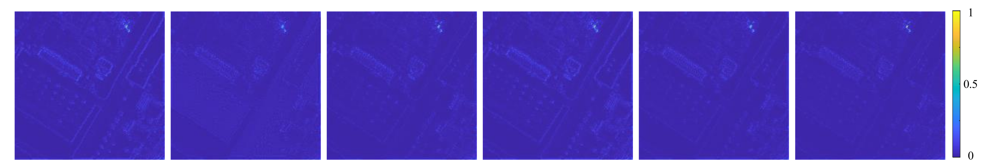
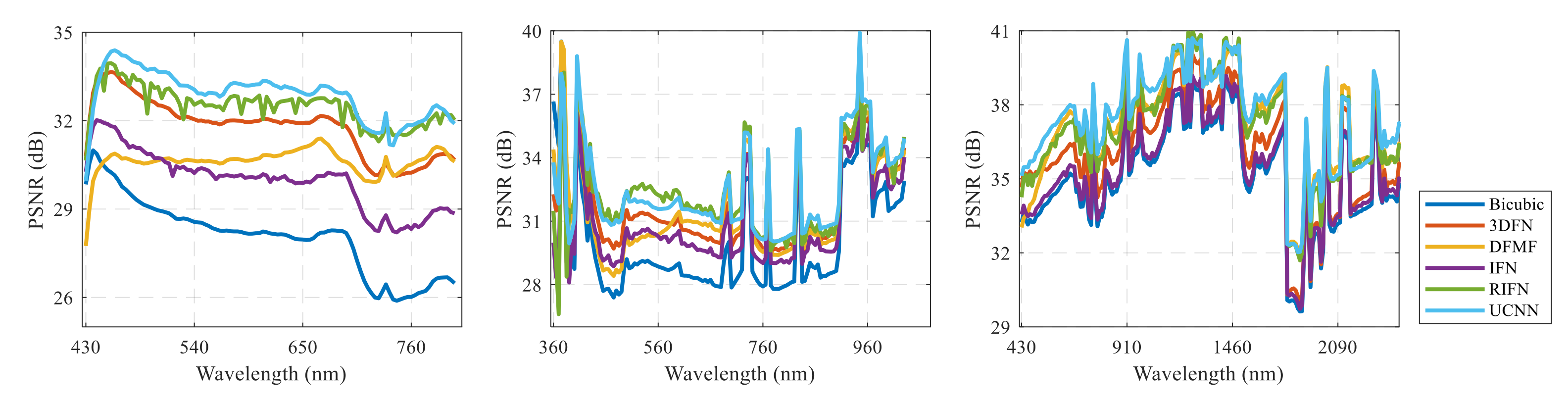
3.2. Results and Analyses

In this work, the experiments were conducted under resolution scales of 2 and 4. The numerical results are tabulated in

Table 2. Numerical evaluation of HS image super-resolution experiments under resolution ratio of 2 ($r=2$).

Dataset	Method	SAM	ERGAS	PSNR (dB)	UIQI	SSIM	Time (s) (Training/Testing)
University of Pavia	Bicubic	4.84	12.60	28.06	0.8969	0.8904	-/0.0101
	3DFN	4.12	8.33	31.79	0.9611	0.9260	45,938.5/2492.9
	DFMF	4.99	10.05	30.62	0.9430	0.9249	1351.7/21.8
	IFN	4.35	10.24	29.97	0.9346	0.9189	1439.1/97.2
	RIFN	3.84	7.84	32.50	0.9651	0.9386	10,385.8/622.7
	UCNN	3.80	7.64	32.74	0.9660	0.9465	2944.5/104.4
University of Houston	Bicubic	6.01	11.90	30.69	0.9323	0.9157	-/0.0150
	3DFN	6.17	9.86	32.17	0.9538	0.9271	66,296.3/3637.2
	DFMF	5.87	9.88	32.20	0.9518	0.9274	1225.7/33.5
	IFN	6.13	11.04	31.26	0.9372	0.9272	1744.8/113.1
	RIFN	5.45	9.47	32.67	0.9481	0.9309	10,740.5/592.2
	UCNN	4.83	9.07	32.85	0.9556	0.9444	2979.4/110.3
San Diego	Bicubic	1.96	7.00	35.21	0.9426	0.9760	-/0.0143
	3DFN	2.34	6.25	36.16	0.9525	0.9811	61,342.4/3172.3
	DFMF	2.38	5.62	37.17	0.9643	0.9823	891.7/24.6
	IFN	2.07	6.81	35.46	0.9467	0.9767	1408.6/109.2
	RIFN	2.42	5.62	37.13	0.9656	0.9827	7665.0/447.1
	UCNN	2.58	5.50	37.33	0.9675	0.9849	2446.6/81.3

and

Table 3. Numerical evaluation of HS image super-resolution experiments under resolution ratio of 4 ($r=4$).

Dataset	Method	SAM	ERGAS	PSNR (dB)	UIQI	SSIM	Time (s) (Training/Testing)
University of Pavia	Bicubic	6.48	8.29	25.64	0.7998	0.8412	-/0.0089
	3DFN	6.28	7.26	26.81	0.8673	0.8629	44,057.7/2394.0
	DFMF	6.77	7.69	26.43	0.8448	0.8603	1138.0/21.4
	IFN	6.07	7.66	26.38	0.8376	0.8563	1469.3/100.3
	RIFN	5.72	7.32	26.76	0.8649	0.8650	10,387.5/563.0
	UCNN	5.57	6.95	27.25	0.8815	0.8772	2976.3/107.7
University of Houston	Bicubic	8.31	7.87	28.34	0.8759	0.8851	-/0.0125
	3DFN	9.16	7.87	28.28	0.8998	0.8794	66,506.2/3413.2
	DFMF	8.05	7.28	28.92	0.8901	0.8972	1186.0/21.8
	IFN	8.55	7.84	28.38	0.8796	0.8870	1771.4/116.6
	RIFN	7.87	7.52	28.86	0.8974	0.8987	10,715.7/577.6
	UCNN	7.21	6.84	29.37	0.9042	0.9071	2964.8/112.8
San Diego	Bicubic	2.59	4.57	32.91	0.8974	0.9652	-/0.0118
	3DFN	3.33	4.42	33.18	0.9132	0.9673	61,124.9/3191.6
	DFMF	2.90	4.37	33.29	0.9119	0.9666	818.5/15.2
	IFN	2.79	4.45	33.14	0.9037	0.9660	1413.4/109.6
	RIFN	2.76	4.30	33.45	0.9146	0.9676	7688.1/477.3
	UCNN	3.10	4.23	33.58	0.9230	0.9703	2387.0/80.0

, where the bold type signifies the best value in each column. By comparing the performance under different downsampling ratios, we could obtain a comprehensive evaluation of the different super-resolution methods. It can be seen that the CNN-based super-resolution approaches generally show higher image fidelity and quality, since, in all cases, the super-resolved images yield lower absolute reconstruction errors (ERGAS) and higher image similarities in both spectral and spatial (PSNR, UIQI, and SSIM) aspects. The bicubic method sometimes has the lowest SAMs (e.g., the San Diego data set). This probably occurs in those scenes with large flattened areas, where the CNN-based super-resolution approaches will lose their advantages in exploring the spatial structure features. Nevertheless, from the following figures, we can also see that, compared with the bicubic method, the CNN methods always have certain advantages in protecting the edges and small objects.

By contrast, in most cases, the proposed UCNN approach achieves the best performance in terms of both spatial and spectral fidelity. For instance, it achieves the lowest SAM values (3.81 and 4.72) in the first two experiments, and the highest PSNR/UIQI/SSIM values (32.87/0.9665/0.9472, 33.00/0.9570/0.9446, and 37.56/0.9682/0.9856, respectively) in all three experiments under $r=2$. Likewise, the lowest ERGAS also indicates the smallest reconstruction error. Similar results can also be clearly observed under $r=4$. This indicates that the super-resolved images of the proposed UCNN are generally closest to the original HS images.

In order to compare the efficiency of these methods, the implementation times of a single run for the raised methods are listed in Table 2 and Table 3. It is widely recognized that the deep learning-based SR methods inevitably take a rather long time for model training. From Table 2 and Table 3, it can be seen that the 3DFN approach is definitely time-consuming, due to its 3D convolutional operations and large patch sizes. RIFN has a very deep residual architecture with 20 convolutional layers. Thus, it also takes hours to train relatively advisable models. It should also be noted that, in our experiments, except for the DFMF method, all the images are first interpolated to the original HS image sizes, before partitioning into sample patches. Therefore, for different resolution ratios, e.g., $r=2$ and $r=4$, the training sets always have the same numbers of samples, and the running times are approximate on the whole. DFMF, however, employs transposed convolutional operations for upscaling, which means that the samples are selected under the degraded scales, resulting in different running times. Essentially, the implementation times of our proposed method are also acceptable among the considered CNN-based methods.

Figure 3, Figure 4 and Figure 5 show the R/G/B color composited images of super-resolved results under $r=2$. Obviously, compared with the references in Figure 2, it can be seen that the bicubic interpolated images commonly have vague edges and blurred details. Undoubtedly, using CNN-based super-resolution approaches indeed enhances the visual details. For instance, we can clearly observe the boundaries and textures of some buildings in the local enlargements. In other words, the spatial resolutions of the HS images have been truly enhanced. From Figure 4, we can also see some subtle differences from the local enlargements, e.g., the second boundary inside the white building can only be observed in Figure 4b,d,f, which indicates that that 3DFN, IRFN, and UCNN have preferable performance in terms of spatial clarity as well.

The overall error maps for different methods are displayed in Figure 6, Figure 7 and Figure 8, which show the absolute values of errors between the super-resolved images and reference images and plot the band average values via the pseudo-color images. For convenience, the values are normalized by the same maximum number for each data set. From these figures, it can be seen that the bicubic method always suffers from large errors, especially at the edges of ground objects, as expected. In contrast, using deep learning techniques, especially the proposed UCNN approach, can effectively reduce the reconstruction errors, as Figure 6, Figure 7 and Figure 8 show, and more importantly, it can enhance the spatial resolution of the images, thereby presenting better appearance and clarity of objects.

Finally, aside from the comparison of spatial clarity in Figure 6, Figure 7 and Figure 8, a brief comparison from the band dimension is exhibited in Figure 9, in which we plot the PSNRs for each band of these super-resolved images. It can be seen that, essentially, the proposed approach has the highest PSNRs for most bands, and RIFN achieves the second-best results, as Table 2 and Table 3 suggest. For the University of Pavia and the University of Houston (under $r=2$), the bicubic method has extremely low PSNRs, resulting in inferior visual effects. In addition, from Figure 9, it can also be seen that some of the spectral bands have relatively higher PSNRs, and the others are much lower. This is mainly caused by the differences in variations between neighboring pixels in different bands. To better illustrate this fact, we plot the average gradient (AG) of each band, for the three reference HS images, in Figure 10. For better comparison, each band is individually normalized to 0~1. AG reflects the differences between neighboring pixels. Therefore, we can see that, for some bands, AGs are much higher than the others, which means that the neighboring pixels are quite different from each other. Hence, the spatial structure information is complicated, and the reconstruction is relatively difficult. A simple example is that, for the bicubic interpolation method, the large difference between neighboring pixels leads to obstruction in the prediction of the center pixel. Moreover, the PSNR is found to be lower accordingly. Combining Figure 9 and Figure 10 can help us to better understand this point.

Nevertheless, the quantitative results and visual effect both demonstrate the effectiveness and superiority of our proposed method over these state-of-the-art works.

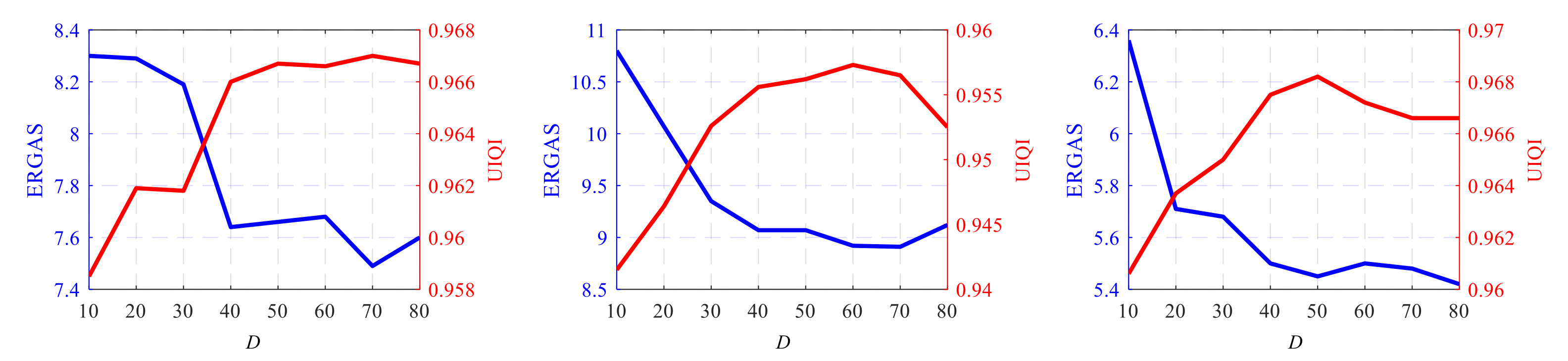
3.3. Discussion of Parameter and Ablation Experiments

In this sub-section, we focus on analyzing the unique parameters and the ablation experiments. In our proposed approach, most of the parameters are determined according to the published references and empirical research, such as the patch size $p$, number of endmembers $D$, learning rate, etc. Therefore, we mainly discuss the results with respect to the balance parameter $\eta$. To this end, Figure 11 and Figure 12 exhibit the ERGAS and UIQI values of the super-resolved and reference images of the testing data, under resolution ratio $r=2$, regarding different $\eta$ and D, respectively. It can be seen that, with the increment of $\eta$ from 0 to 1, the ERGAS essentially declines slightly to the minimum values and then rises continuously. Conversely, the UIQI climbs to the relative maximum values first, and then drops. A smaller $\eta$ is generally more satisfactory than a larger one. We believe that a relatively optimal $\eta$ that minimizes the spectral distortions and maximizes the performance of image super-resolution is around 0.2 in our presented experiments. Therefore, in this work, we set $\eta$ to 0.2, 0.4, and 0.2, for the three data sets, respectively, in the previous sub-section. Likewise, Figure 12 shows the results with respect to different numbers of endmembers D. It can be seen that satisfactory results can be achieved when D ≥ 40. The relatively optimal values are achieved when D is around 50~60. When D < 40, the super-resolved results seem to be unacceptable, especially when D < 20. For the sake of fairness and generality, in this work, we set D = 40 in the previous sub-section. The results under $r=4$ in Table 2 and Table 3 demonstrate that the two values are also feasible to some extent, and can achieve acceptable results. Nevertheless, we should also point out that the selection of the two $\eta$ and D in this work actually depends on our empirical knowledge with extensive experiments and tests. However, we have not developed adaptive rules to automatically determine these two parameters. Therefore, our following work will focus on the automatic determination of $\eta$ and D—for example, using the automatic estimation approaches of endmember numbers in [48,49,50].

Aside from the above analysis of parameters, we also present a brief discussion of the ablation experiments to analyze the mechanism of our proposed approach. To this end, we considered four demoted versions of our proposed approach. In the first case, which is denoted by Case 1, the network was employed to directly predict the HR abundance maps, only by the lower branch of Figure 1, with the same parameters (i.e., $\eta$, $D$, etc.) as the proposed approach. The spatial correlation was also omitted. In the second case, the entire network of Figure 1 was used to simultaneously predict the LR and HR abundance maps. However, unlike Case 1 and the proposed method, the endmember update operation in (8) was not applied, which means that the endmember remained invariant in the training and testing stages. The parameters were also set the same as in UCNN. This is denoted by Case 2. The third case was almost the same as the proposed method, but we arbitrarily set $\eta$ to 0 during the training stage, which is the same case as the first points in Figure 11. This is denoted by Case 3. In the last case, which is denoted by Case 4, the training manner was almost the same as in UCNN, but in the testing phase, the entire LR HS image with the original size was input into the network to directly predict the abundance maps with the original size, instead of using partitioned patches. Obviously, this method requires much less time for the testing phase, since only a single forward propagation operation is implemented.

The experimental results of the three above-mentioned cases are reported in Figure 13, as well as the proposed approach. Obviously, from Figure 13, we can see that the proposed UCNN remains the best one in terms of both spectral fidelity and image quality. By comparing Case 1 and UCNN, it is apparent that incorporating the spatial correlation between HR and LR HS images into network learning indeed provides a favorable outcome, i.e., relatively lower ERGASs and higher UIQIs in all cases, with a limited increment in computation. Moreover, in the testing stage of HR abundances, in the upper branch of Figure 1, the prediction of LR abundances is no longer needed, which further reduces the computation time. Second, it can be inferred that the update of endmembers is indispensable, since the results of Case 2 deteriorated severely, e.g., in the left upper and right lower figures, Case 2 has a very high ERGAS value, with a much lower UIQI, compared with UCNN and the others. Fortunately, the update of endmembers requires much less time than the backward propagation in network training. Third, combing the results in Figure 11 and Figure 13, it can be seen that the involvement of abundance sparsity will also have a minor effect on the performance. A proper sparsity $\eta$ can further reduce the errors, enhance the image quality, and benefit the fidelity of super-resolved images, without any additional computation requirements. Lastly, by comparing the results of Case 4 and UCNN, it can also be concluded that predicting small pieces of patches provides more accurate results than the entire LR HS image with the original size, although more time may be needed for forward propagations.

In summary, the experiments demonstrate that the update rule of endmembers is crucial to the accuracy of image reconstruction. Meanwhile, the regularization of spatial correlation between LR and HR images, namely the prediction of LR abundances, will truly benefit the inference of HR abundances and HS images. Furthermore, it is also worth noting that the quantity and diversity of samples are also quite important to the CNN-based super-resolution approaches. In our future work, we will also aim to promote the quality and quantity of samples so that we can train more robust and effective networks to handle various scenes.

4. Conclusions

In this paper, a super-resolution approach based on a convolutional neural network is proposed, aiming to spatially enhance the resolution of HS images, without the aid of auxiliary sources. The proposed method takes advantage of the spectral mixture model and the spatial spread transform model. It thus employs the spatial correlation-regularized CNN to predict the desired high-resolution abundance maps, thereby reconstructing the high-resolution HS image. Experimental results on three public HS images demonstrate that the proposed approach can effectively enhance the spatial details and exhibit high spectral fidelity, compared with several state-of-the-art SR methods, from both visual effects and quantitative evaluations. The ablation experiments also demonstrate that the proposed network architecture and spatial correlation regularization can further improve the spectral quality of super-resolved images. Meanwhile, in this paper, we have also analyzed the influences of two important parameters, namely the balance parameter η and number of endmembers D. However, it should be pointed out that, in this work, the selection of parameters essentially depends on our empirical knowledge and extensive experiments. Therefore, our next work will focus on enhancing the adaptability of our approach by automatically determining the parameters. We will also make efforts to improve the quality and quantity of training samples to handle various scenes, and expedite the network training procedure.

References

1. Selva, M.; Aiazzi, B.; Butera, F.; Chiarantini, L.; Baronti, S. Hyper-sharpening: A first approach on sim-ga data. IEEE J. Sel. Top. Appl. Earth Obs. Remote Sens. 2015, 8, 3008–3024. [Google Scholar] [CrossRef]
2. Lu, X.; Zhang, J.; Li, T.; Zhang, Y. Pan-sharpening by multilevel interband structure modeling. IEEE Geosci. Remote Sens. Lett. 2016, 13, 892–896. [Google Scholar] [CrossRef]
3. Li, X.; Yuan, Y.; Wang, Q. Hyperspectral and multispectral image fusion based on band simulation. IEEE Geosci. Remote Sens. Lett. 2020, 17, 479–483. [Google Scholar] [CrossRef]
4. Palsson, F.; Sveinsson, J.R.; Ulfarsson, M.O.; Benediktsson, J.A. Model-based fusion of multi- and hyperspectral images using pca and wavelets. IEEE Trans. Geosci. Remote Sens. 2015, 53, 2652–2663. [Google Scholar] [CrossRef]
5. Wei, Q.; Dobigeon, N.; Tourneret, J.; Bioucas-Dias, J.; Godsill, S. R-fuse: Robust fast fusion of multiband images based on solving a sylvester equation. IEEE Signal Process Lett. 2016, 23, 1632–1636. [Google Scholar] [CrossRef] [Green Version]
6. Yokoya, N.; Yairi, T.; Iwasaki, A. Coupled nonnegative matrix factorization unmixing for hyperspectral and multispectral data fusion. IEEE Trans. Geosci. Remote Sens. 2012, 50, 528–537. [Google Scholar] [CrossRef]
7. Karoui, M.S.; Deville, Y.; Benhalouche, F.Z.; Boukerch, I. Hypersharpening by joint-criterion nonnegative matrix factorization. IEEE Trans. Geosci. Remote Sens. 2017, 55, 1660–1670. [Google Scholar] [CrossRef]
8. Li, S.; Dian, R.; Fang, L.; Bioucas-Dias, J.M. Fusing hyperspectral and multispectral images via coupled sparse tensor factorization. IEEE Trans. Image Process. 2018, 27, 4118–4130. [Google Scholar] [CrossRef]
9. Dian, R.; Li, S.; Fang, L. Learning a low tensor-train rank representation for hyperspectral image super-resolution. IEEE Trans. Neural Netw. Learn. Syst. 2019, 30, 2672–2683. [Google Scholar] [CrossRef]
10. Dian, R.; Li, S.; Guo, A.; Fang, L. Deep hyperspectral image sharpening. IEEE Trans. Neural Netw. Learn. Syst. 2018, 29, 5345–5355. [Google Scholar] [CrossRef] [PubMed]
11. Qi, X.; Zhou, M.; Zhao, Q.; Meng, D.; Zuo, W.; Xu, Z. Multispectral and Hyperspectral Image Fusion by MS/HS Fusion Net. In Proceedings of the IEEE Conference on Computer Vision and Pattern Recognition (CVPR), Long Beach, CA, USA, 16–20 June 2019. [Google Scholar] [CrossRef] [Green Version]
12. Xu, S.; Amira, O.; Liu, J.; Zhang, C.; Zhang, J.; Li, G. Ham-mfn: Hyperspectral and multispectral image multiscale fusion network with rap loss. IEEE Trans. Geosci. Remote Sens. 2020, 58, 4618–4628. [Google Scholar] [CrossRef]
13. Zheng, K.; Gao, L.; Liao, W.; Hong, D.; Zhang, B.; Cui, X.; Chanussot, J. Coupled convolutional neural network with adaptive response function learning for unsupervised hyperspectral super resolution. IEEE Trans. Geosci. Remote Sens. 2021, 59, 2487–2502. [Google Scholar] [CrossRef]
14. Simões, M.; Bioucas-Dias, J.; Almeida, L.B.; Chanussot, J. A convex formulation for hyperspectral image superresolution via subspace-based regularization. IEEE Trans. Geosci. Remote Sens. 2015, 53, 3373–3388. [Google Scholar] [CrossRef] [Green Version]
15. Nezhad, Z.H.; Karami, A.; Heylen, R.; Scheunders, P. Fusion of hyperspectral and multispectral images using spectral unmixing and sparse coding. IEEE J. Sel. Top. Appl. Earth Obs. Remote Sens. 2016, 9, 2377–2389. [Google Scholar] [CrossRef]
16. Xing, C.; Wang, M.; Dong, C.; Duan, C.; Wang, Z. Joint sparse-collaborative representation to fuse hyperspectral and multispectral images. Signal Process. 2020, 173, 107585. [Google Scholar] [CrossRef]
17. Loncan, L.; De Almeida, L.B.; Bioucas-Dias, J.M.; Briottet, X.; Chanussot, J.; Dobigeon, N.; Fabre, S.; Liao, W.; Licciardi, G.A.; Simões, M.; et al. Hyperspectral pansharpening: A review. IEEE Geosci. Remote Sens. Mag. 2015, 3, 27–46. [Google Scholar] [CrossRef] [Green Version]
18. Yokoya, N.; Grohnfeldt, C.; Chanussot, J. Hyperspectral and multispectral data fusion: A comparative review of the recent literature. IEEE Geosci. Remote Sens. Mag. 2017, 5, 29–56. [Google Scholar] [CrossRef]
19. Dian, R.; Li, S.; Sun, B.; Guo, A. Recent advances and new guidelines on hyperspectral and multispectral image fusion. Inf. Fusion 2021, 69, 40–51. [Google Scholar] [CrossRef]
20. Lu, X.; Zhang, J.; Yu, X.; Tang, W.; Li, T.; Zhang, Y. Hyper-sharpening based on spectral modulation. IEEE J. Sel. Top. Appl. Earth Obs. Remote Sens. 2019, 12, 1534–1548. [Google Scholar] [CrossRef]
21. Borsoi, R.A.; Imbiriba, T.; Bermudez, J.C.M. Super-resolution for hyperspectral and multispectral image fusion accounting for seasonal spectral variability. IEEE Trans. Image Process. 2020, 29, 116–127. [Google Scholar] [CrossRef] [PubMed] [Green Version]
22. Dong, C.; Loy, C.C.; He, K.; Tang, X. Image super-resolution using deep convolutional networks. IEEE Trans. Pattern Anal. Mach. Intell. 2016, 38, 295–307. [Google Scholar] [CrossRef] [PubMed] [Green Version]
23. Wang, L.; Huang, Z.; Gong, Y.; Pan, C. Ensemble based deep networks for image super-resolution. Pattern Recognit. 2017, 68, 191–198. [Google Scholar] [CrossRef]
24. Akgun, T.; Altunbasak, Y.; Mersereau, R.M. Super-resolution reconstruction of hyperspectral images. IEEE Trans. Image Process. 2005, 14, 1860–1875. [Google Scholar] [CrossRef] [PubMed]
25. Patel, R.C.; Joshi, M.V. Super-resolution of hyperspectral images: Use of optimum wavelet filter coefficients and sparsity regularization. IEEE Trans. Geosci. Remote Sens. 2015, 53, 1728–1736. [Google Scholar] [CrossRef]
26. Li, J.; Yuan, Q.; Shen, H.; Meng, X.; Zhang, L. Hyperspectral image super-resolution by spectral mixture analysis and spatial–spectral group sparsity. IEEE Geosci. Remote Sens. Lett. 2016, 13, 1250–1254. [Google Scholar] [CrossRef]
27. Dong, W.; Fu, F.; Shi, G.; Cao, X.; Wu, J.; Li, G.; Li, X. Hyperspectral image super-resolution via non-negative structured sparse representation. IEEE Trans. Image Process. 2016, 25, 2337–2352. [Google Scholar] [CrossRef] [PubMed]
28. Irmak, H.; Akar, G.B.; Yuksel, S.E. A map-based approach for hyperspectral imagery super-resolution. IEEE Trans. Image Process. 2018, 27, 2942–2951. [Google Scholar] [CrossRef]
29. Hong, D.; He, W.; Yokoya, N.; Yao, J.; Gao, L.; Zhang, L.; Chanussot, J.; Zhu, X. Interpretable hyperspectral artificial intelligence: When nonconvex modeling meets hyperspectral remote sensing. IEEE Geosci. Remote Sens. Mag. 2021, 9, 52–87. [Google Scholar] [CrossRef]
30. Lai, W.; Huang, J.; Ahuja, N.; Yang, M. Deep Laplacian pyramid networks for fast and accurate super-resolution. In Proceedings of the IEEE Conference on CVPR, Honolulu, HI, USA, 21–26 July 2017; pp. 5835–5843. [Google Scholar] [CrossRef] [Green Version]
31. Lai, W.; Huang, J.; Ahuja, N.; Yang, M. Fast and accurate image super-resolution with deep Laplacian pyramid networks. IEEE Trans. Pattern Anal. Mach. Intell. 2019, 41, 2599–2613. [Google Scholar] [CrossRef] [PubMed] [Green Version]
32. Hu, J.; Li, Y.; Xie, W. Hyperspectral image super-resolution by spectral difference learning and spatial error correction. IEEE Geosci. Remote Sens. Lett. 2017, 14, 1825–1829. [Google Scholar] [CrossRef]
33. Mei, S.; Yuan, X.; Ji, J.; Zhang, Y.; Wan, S.; Du, Q. Hyperspectral image spatial super-resolution via 3d full convolutional neural network. Remote Sens. 2017, 9, 1139. [Google Scholar] [CrossRef] [Green Version]
34. Arun, P.V.; Buddhiraju, K.M.; Porwal, A.; Chanussot, J. Cnn-based super-resolution of hyperspectral images. IEEE Trans. Geosci. Remote Sens. 2020, 58, 6106–6121. [Google Scholar] [CrossRef]
35. Hu, J.; Tang, Y.; Fan, S. Hyperspectral image super resolution based on multiscale feature fusion and aggregation network with 3-d convolution. IEEE J. Sel. Top. Appl. Earth Obs. Remote Sens. 2020, 13, 5180–5193. [Google Scholar] [CrossRef]
36. Xie, W.; Jia, X.; Li, Y.; Lei, J. Hyperspectral image super-resolution using deep feature matrix factorization. IEEE Trans. Geosci. Remote Sens. 2019, 57, 6055–6067. [Google Scholar] [CrossRef]
37. Zou, C.; Huang, X. Hyperspectral image super-resolution combining with deep learning and spectral unmixing. Signal Process. Image Commun. 2020, 84, 115833. [Google Scholar] [CrossRef]
38. Li, J.; Cui, R.; Li, B.; Song, R.; Li, Y.; Dai, Y.; Du, Q. Hyperspectral image super-resolution by band attention through adversarial learning. IEEE Trans. Geosci. Remote Sens. 2020, 58, 4304–4318. [Google Scholar] [CrossRef]
39. Hu, J.; Jia, X.; Li, Y.; He, G.; Zhao, M. Hyperspectral image super-resolution via intrafusion network. IEEE Trans. Geosci. Remote Sens. 2020, 58, 7459–7471. [Google Scholar] [CrossRef]
40. Hu, J.; Zhao, M.; Li, Y. Hyperspectral image super-resolution by deep spatial-spectral exploitation. Remote Sens. 2019, 11, 1229. [Google Scholar] [CrossRef] [Green Version]
41. Jiang, J.; Sun, H.; Liu, X.; Ma, J. Learning spatial-spectral prior for super-resolution of hyperspectral imagery. IEEE Trans. Comput. Imaging 2020, 6, 1082–1096. [Google Scholar] [CrossRef]
42. Fu, Y.; Liang, Z.; You, S. Bidirectional 3d quasi-recurrent neural network for hyperspectral image super-resolution. IEEE J. Sel. Top. Appl. Earth Obs. Remote Sens. 2021, 14, 2674–2688. [Google Scholar] [CrossRef]
43. Shi, Q.; Tang, X.; Yang, T.; Liu, R.; Zhang, L. Hyperspectral image denoising using a 3-D attention denoising network. IEEE Trans. Geosci. Remote Sens. 2021, 1–16. [Google Scholar] [CrossRef]
44. Dou, X.; Li, C.; Shi, Q.; Liu, M. Super-resolution for hyperspectral remote sensing images based on the 3D attention-SRGAN network. Remote Sens. 2020, 12, 1204. [Google Scholar] [CrossRef] [Green Version]
45. Liu, M.; Shi, Q.; Marinori, A.; He, D.; Liu, X.; Zhang, L. Super-resolution-based change detection network with stacked attention module for images with different resolutions. IEEE Trans. Geosci. Remote Sens. 2021. [Google Scholar] [CrossRef]
46. Li, K.; Yang, S.H.; Dong, R.T.; Wang, X.Y.; Huang, J.Q. Survey of single image super-resolution reconstruction. IET Image Process 2020, 14, 2273–2290. [Google Scholar] [CrossRef]
47. Lu, X.; Li, T.; Zhang, J.; Jia, F. A novel unmixing-based hypersharpening method via convolutional neural network. IEEE Trans. Geosci. Remote Sens. 2021, 1–14. [Google Scholar] [CrossRef]
48. Zhu, X.; Kang, Y.; Liu, J. Estimation of the number of endmembers via thresholding ridge ratio criterion. IEEE Trans. Geosci. Remote Sens. 2020, 58, 637–649. [Google Scholar] [CrossRef]
49. Prades, J.; Safont, G.; Salazar, A.; Vergara, L. Estimation of the number of endmembers in hyperspectral images using agglomerative clustering. Remote Sens. 2020, 12, 3585. [Google Scholar] [CrossRef]
50. Wang, X.; Zhong, Y.; Cui, C.; Zhang, L.; Xu, Y. Autonomous endmember detection via an abundance anomaly guided saliency prior for hyperspectral imagery. IEEE Trans. Geosci. Remote Sens. 2021, 59, 2336–2351. [Google Scholar] [CrossRef]
51. Liu, D.; Li, J.; Yuan, Q. A spectral grouping and attention-driven residual dense network for hyperspectral image super-resolution. IEEE Trans. Geosci. Remote Sens. 2020, 1–15. [Google Scholar] [CrossRef]
52. Lu, X.; Zhang, J.; Yang, D.; Xu, L.; Jia, F. Cascaded convolutional neural network-based hyperspectral image resolution enhancement via an auxiliary panchromatic image. IEEE Trans. Image Process. 2021, 30, 6815–6828. [Google Scholar] [CrossRef]
Figure 1. The main framework of the proposed HS image super-resolution approach.
Remotesensing 13 04074 g001
Figure 2. Experimental data sets. (a) Training image of University of Pavia; (b) Testing image of University of Pavia; (c) Training image of University of Houston; (d) Testing image of University of Houston; (e) Training image of San Diego air station; (f) Testing image of San Diego air station.
Remotesensing 13 04074 g002
Figure 3. Super-resolved images of University of Pavia data set. (a) Bicubic; (b) 3DFN; (c) DFMF; (d) IFN; (e) RIFN; (f) UCNN.
Remotesensing 13 04074 g003
Figure 4. Super-resolved images of University of Houston data set. (a) Bicubic; (b) 3DFN; (c) DFMF; (d) IFN; (e) RIFN; (f) UCNN.
Remotesensing 13 04074 g004
Figure 5. Super-resolved images of San Diego data set. (a) Bicubic; (b) 3DFN; (c) DFMF; (d) IFN; (e) RIFN; (f) UCNN.
Remotesensing 13 04074 g005
Figure 6. Band averages of absolute errors of University of Pavia data set. (From left to right: Bicubic, 3DFN, DFMF, IFN, RIFN, UCNN).
Remotesensing 13 04074 g006
Figure 7. Band averages of absolute errors of University of Houston data set. (From left to right: Bicubic, 3DFN, DFMF, IFN, RIFN, UCNN).
Remotesensing 13 04074 g007
Figure 8. Band averages of absolute errors of San Diego data set. (From left to right: Bicubic, 3DFN, DFMF, IFN, RIFN, UCNN).
Remotesensing 13 04074 g008
Figure 9. PSNRs for each band of the super-resolved images. (The upper line is under r = 2, and the lower line is under r = 4. From left to right: University of Pavia, University of Houston, and San Diego air station).
Remotesensing 13 04074 g009aRemotesensing 13 04074 g009b
Figure 10. Average gradient of each band for the reference images. (From left to right: University of Pavia, University of Houston, and San Diego air station).
Remotesensing 13 04074 g010
Figure 11. The ERGAS and UIQI values with respect to η of UCNN. (From left to right: University of Pavia, University of Houston, and San Diego air station).
Remotesensing 13 04074 g011
Figure 12. The ERGAS and UIQI values with respect to number of endmembers D. (From left to right: University of Pavia, University of Houston, and San Diego air station).
Remotesensing 13 04074 g012
Figure 13. Comparison of ERGAS and UIQI values with respect to different structures of the proposed methods. (The upper line is under r = 2, and the lower line is under r = 4. From left to right: University of Pavia, University of Houston, and San Diego air station).
Remotesensing 13 04074 g013