Situational Awareness of Large Infrastructures Using Remote Sensing: The Rome–Fiumicino Airport during the COVID-19 Lockdown

Abstract

Situational awareness refers to the process of aggregating spatio-temporal variables and measurements from different sources, aiming to improve the semantic outcome. Remote Sensing satellites for Earth Observation acquire key variables that, when properly aggregated, can provide precious insights about the observed area. This article introduces a novel automatic system to monitor the activity levels and the operability of large infrastructures from satellite data. We integrate multiple data sources acquired by different spaceborne sensors, such as Sentinel-1 Synthetic Aperture Radar (SAR) time series, Sentinel-2 multispectral data, and Pleiades Very-High-Resolution (VHR) optical data. The proposed methodology exploits the synergy between these sensors for extracting, at the same time, quantitative and qualitative results. We focus on generating semantic results, providing situational awareness, and decision-ready insights. We developed this methodology for the COVID-19 Custom Script Contest, a remote hackathon funded by the European Space Agency (ESA) and the European Commission (EC), whose aim was to promote remote sensing techniques to monitor environmental factors consecutive to the spread of the Coronavirus disease. This work focuses on the Rome–Fiumicino International Airport case study, an environment significantly affected by the COVID-19 crisis. The resulting product is a unique description of the airport’s area utilization before and after the air traffic restrictions imposed between March and May 2020, during Italy’s first lockdown. Experimental results confirm that the proposed algorithm provides remarkable insights for supporting an effective decision-making process. We provide results about the airport’s operability by retrieving temporal changes at high spatial and temporal resolutions, together with the airplane count and localization for the same period in 2019 and 2020. On the one hand, we detected an evident change of the activity levels on those airport areas typically designated for passenger transportation, e.g., the one close to the gates. On the other hand, we observed an intensification of the activity levels over areas usually assigned to landside operations, e.g., the one close to the hangar. Analogously, the airplane count and localization have shown a redistribution of the airplanes over the whole airport. New parking slots have been identified as well as the areas that have been dismissed. Eventually, by combining the results from different sensors, we could affirm that different airport surface areas have changed their functionality and give a non-expert interpretation about areas’ usage.

1. Introduction

The definition of Situational Awareness (SA) commonly refers to the process of understanding a set of ongoing phenomena related to a specific environment and their evolution in space and time [1,2]. The academic literature sets SA as a separation line between the human understanding of the system status and the actual one [1]. The first research activities in the field were boosted by the aviation industry, particularly for maintaining the safe control of an aircraft [3,4]. Indeed, while flying an aircraft from one place to another, pilots must perform a wide range of tasks, including fast decision-making and development of self-judgments about the mission performance [5]. Similarly, air traffic control specialists have to make difficult decisions under time pressure, high workload, and by considering a dynamic environment evolving according to a plurality of factors [6].

In the Earth Observation (EO) field, there is a large variety of Remote Sensing (RS) data sets that represent a precious resource for SA applications. RS actually plays a central role for the interpretation of the environment and can be used as an auxiliary tool for an effective decision-making [7,8,9,10,11]. The RS analyst derives information from RS data to reduce the uncertainties associated with standard geospatial intelligence. Thanks to the RS analyst’s mathematical and physical techniques, the decision-maker selects between uncertain outcomes to optimize expected value or utility [8]. Over the past two decades, many studies developed in the USA and Europe have demonstrated that fast network connectivity is essential to efficiently transfer products from data providers to stakeholders and decision-makers [7,12]. Indeed, it ensures the availability of low-cost periodic remote sensing products on which even decision-makers may comment with the RS analysts for application development success. A typical example of the application of remote sensing to decision-making is the adoption of precision farming in the management of croplands. A work made in 2003 by the University of North Dakota, within the NASA’s Synergy program, provided several farmers with multi-spectral data throughout the growing season [7]. The result was extremely positive: those farmers who relied on satellite imagery for variable rate application of nitrogen reported a saving of 12 $ per acre in fertilizer costs, reducing, at the same time, the environmental contamination. Further SA applications from the Synergy program concern

• the monitoring of the evapotranspiration, i.e., vapor contribution of plants and oceans to the atmosphere, in the Snake River Aquifer in Southern Idaho;
• the estimating snow water equivalent, i.e., the equivalent amount of liquid water stored in the snowpack, in Arizona; and
• the determination of runoff coefficient maps for use in models to measure peak flood discharges in Missouri [7].

In Europe, the German Aerospace Center (DLR) has been involved since 2014 in SA activities through the VABENE++ project. This early-warning system exploits airborne remote sensing and in situ data collections for providing terrestrial traffic data. This service aids public offices and organizations with security responsibilities and traffic authorities when dealing with disasters and large public events [9]. As an example, more recently, in 2019, DLR organized a test in The Hague, The Netherlands, for assessing the role of VABENE++ to support disaster response tasks in a large-scale flooding scenario [11].

The latest developments in Remote Sensing for Earth Observation foresee the implementation of various innovative satellite constellations. Among these, we can include already existing and very successful realities as, for example, the multiple-platform Synthetic Aperture Radar (SAR) and the Very-High-Resolution (VHR) optical sensors constellations from ICEEYE and Planet companies, respectively. Future scenarios will also include spaceborne missions suitable for increased coverage and revisit time, providing high spatial and temporal resolution. This trend will enable a large variety of techniques that require higher temporal and spatial resolution data for Situational Awareness applications.

During the COVID-19 outbreak, governments worldwide were forced to take prompt and drastic decisions to limit the virus’s pandemic outbreak. The planning of a second phase and the return to everyday life went through the reopening of infrastructures, such as ports, stadiums, marinas, airports, and tourist places [13]. The monitoring of large infrastructures is therefore of strategic importance to control mobility and gathering of people and to accordingly react with restrictions or, on the contrary, to allow for a relaxation of the social distancing rules [14,15,16]. This situation has fastened RS systems’ development to monitor crucial parameters related to the impacts on natural variables, human activity distribution, and economy consequent to the COVID-19 pandemic. The main research activities have focused on determining the impact of control measures and the consequent reduced human activities on natural variables as air and water quality. The former has been assessed in [17,18,19,20] by exploiting the TROPOspheric Monitoring Instrument (TROPOMI) [21] and the MODerate resolution Imaging Spectrometer (MODIS) [22]. Other research studies, instead, explicitly focused on Nitrogen Dioxide measurements [23,24]. Light pollution has also been considered in [25,26] as it is directly linked to air quality measurements. In [27], instead, the authors developed a methodology for monitoring water quality by measuring turbidity levels from the inversion of the amount of total suspended matter from PlanetScope VHR optical imagery. Closer to SA systems, the methodology used in [28] provides a broad overview of key environmental parameters and the link to their economic impact by exploiting the data combination of Daily-Night Band (DNB) optical imagery, cellular mobile data, and NO2 TROPOMI Instrument. Similarly, in [29], the authors propose a system for monitoring human activities and their consequent effect on the environment by analyzing a combination of Night-Time Light (NTL) radiance level and Air Quality Index (AQI) before and after the pandemic. Eventually, a methodology devoted to Situational Awareness and based on SAR data has been developed in [30]. In this paper, the authors proposed to use SAR images to detect moving vehicles such as cars, trucks, and buses, and, eventually, monitor the traffic pattern over time. This technique exploits the across-track shift present in SAR data when a moving target has a relative movement in the across-track direction with respect to the sensor’s orbiting platform.

The European Commission (EC) and the European Space Agency (ESA) have put in action an online platform, namely, the Rapid Action on Coronavirus and EO (RACE), aiming at providing prompt insights on crucial natural and economic indicators [31]. The latter includes the amount of activity over commercial centers, truck activities over highways and production sites, and, last but not least, over airports. This initiative highlights the importance of having a centralized informational platform for collecting, reporting, and combining EO results for providing situational awareness insights at a large/global scale. In this framework, we now focus on the usability of semantic results extracted from remote sensing data to facilitate and accelerate the decision-making process and adjust restrictions to dynamic pandemic changes. For this purpose, we implemented an automatic system for the monitoring of large infrastructures by exploiting the synergies between Sentinel-1 (S-1) SAR time-series, Sentinel-2 (S-2) High-Resolution (HR) multispectral data, and Pleiades VHR optical data. In the following, we refer to our methodology as STAND-OUT: SituaTional Awareness of large iNfrastructures during the coviD OUTbreak. As a case study, we focus on the Rome–Fiumicino International Airport, whose economic and logistic importance makes it an ideal test site for assessing the proposed methodology. Over this area, two Pleiades acquisitions, in 2019 and 2020, have been made available during the COVID-19 Custom Script Contest [32] and are here exploited to prove the efficiency of STAND-OUT. In particular, we aim at monitoring the level of ongoing activity due to human operations over dedicated areas of the airport, using free of charge products provided by the Sentinel fleet.

This article sets the groundwork for future SA systems, which will benefit from higher resolution and will provide timely and highly accurate insights to enhance real tasks such as (1) security and management in economic activities (e.g., transport networks and commercial areas), (2) food security and safety in agricultural activities (e.g., understanding of unattended fields and crops and detection of disruptions due to supply chain issues), and (3) monitoring of human activities (e.g., social distancing estimations and parked car distributions over dense urban areas). We organized the paper into five sections. Section 2 presents the materials used in this work, i.e., data sets, acquisition dates, test areas, and acquisition IDs, for the data from the Sentinel fleet, Pleiades, and the in situ measurements. Then, Section 3 describes step-by-step the STAND-OUT automatic algorithm. The results and discussion are reported in Section 4. Finally, the conclusions are drawn in Section 5.

2. Materials

This section describes the selected test site, the exploited in situ information, and the remotely sensed imagery data set, which comprises Sentinel-1, Sentinel-2, and Pleiades acquisitions. We point out that, while the presented methodology stands for any infrastructure monitoring, specific in situ measurements may vary depending on the final application.

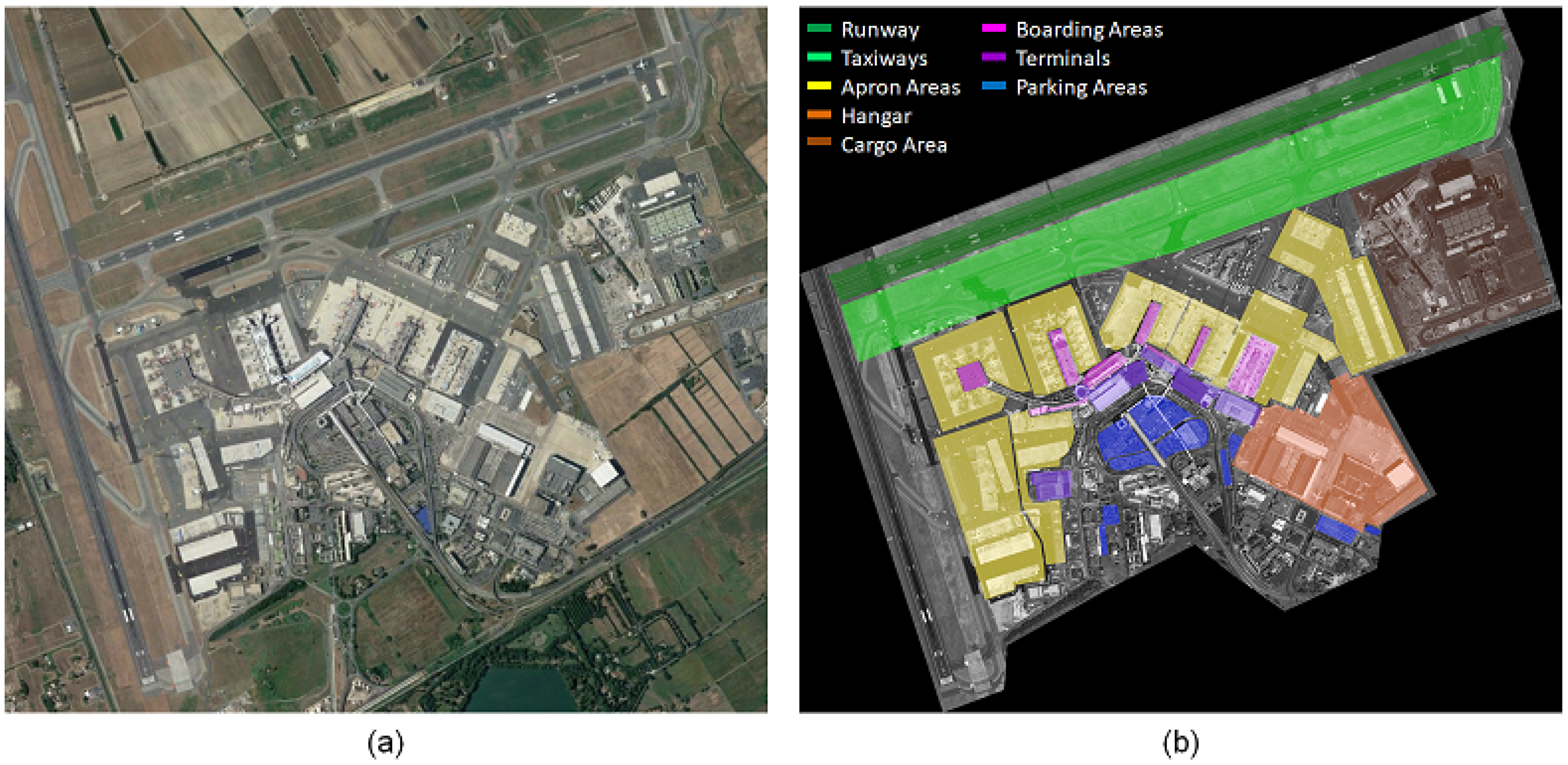
2.1. Test Site: Rome–Fiumicino International Airport

We consider the Rome–Fiumicino International Airport as a case study for the presented methodology. This airport is the largest in Italy and covers an area of about 16 km${}^2$. In Figure 1b, we can observe that the airport comprises five terminal buildings (purple), eight apron areas (yellow), one hangar (orange) of 450 m${}^2$, and a dedicated Cargo City terminal (brown). Its operability has been strongly affected after the recent COVID-19 outbreak, making it the ideal environment for testing the proposed methodology. In particular, some terminals were fully suspended [33], and different airport areas changed their functionalities.

While the former is relatively well documented on the official website, the latter results more challenging to prove since internal documents are not easily accessible. In this context, we considered the map retrieved from official documents available online [34] and depicted in Figure 2a.

By combining the apron areas in Figure 2a together with the hangar, we created a set of masks, each one defining a parking area located on separate sides of the Fiumicino airport. The final result, shown in Figure 2b, has been used as in-situ measurement for assessing STAND-OUT.

2.2. Sentinel-1 Time Series

We downloaded and processed a S-1 time series within the area of interest, covering four months across Italy’s lockdown starting date (9 March 2020). Therefore, to highlight the effects of the airport restrictions, we selected a second S-1 time series on the same time frame (between January and May) but in 2019.

Table 1. Sentinel-1 acquisitions selected for the 2019 and 2020 stacks.

Sentinel-1: List of Acquisitions
Mode	Product Type	Rel. Orbit	Orbit Direction	Polarization
IW	GRD	117	Ascending	VV/VH
Stack 2019			Stack 2020
Sensing Date	Sensor Name	ID	Sensing Date	Sensor Name	ID
2 January 2019	S-1B	47EE	3 January 2020	S-1A	5D72
8 January 2019	S-1A	CB9E	9 January 2020	S-1B	E551
14 January 2019	S-1B	3CC5	15 January 2020	S-1A	2FEC
20 January 2019	S-1A	06FE	21 January 2020	S-1B	9DD5
26 January 2019	S-1B	6BAC	27 January 2020	S-1A	A254
1 February 2019	S-1A	F94E	missed
7 February 2019	S-1B	A5D4	8 February 2020	S-1A	A28B
13 February 2019	S-1A	A3D1	14 February 2020	S-1B	13D3
19 February 2019	S-1B	A527	20 February 2020	S-1A	4DDB
25 February 2019	S-1A	F427	26 February 2020	S-1B	55EB
3 March 2019	S-1B	6D76	3 March 2020	S-1A	1432
9 March 2019	S-1A	5CC6	9 March 2020	S-1B	5AB7
15 March 2019	S-1B	F704	15 March 2020	S-1A	D5CF
21 March 2019	S-1A	ABAA	21 March 2020	S-1B	B491
27 March 2019	S-1B	DC1F	27 March 2020	S-1A	67DD
2 April 2019	S-1A	7D8E	2 April 2020	S-1B	5BC1
8 April 2019	S-1B	7B3E	8 April 2020	S-1A	A470
14 April 2019	S-1A	E962	14 April 2020	S-1B	86A6
20 April 2019	S-1B	0320	29 April 2020	S-1A	3A98
26 April 2019	S-1A	16DC	26 April 2020	S-1B	2CEE
2 May 2019	S-1B	889E	2 May 2020	S-1A	4ED2
8 May 2019	S-1A	D64D	8 May 2020	S-1B	3FD5

details the complete acquisitions exploited in this work. For the sake of simplicity, we defined the two time series as Stack 2020 and Stack 2019, respectively. In this work, we considered the Ground Range Detected (GRD) products acquired by both satellite units of the fleet: Sentinel-1A (S-1A) and Sentinel-1B (S-1B). Operating in the Interferometric Wide (IW) swath mode, the twin S-1 satellites fly in the same orbital plane ${180}^{\circ }$ out of phase with each other, covering Europe with a short revisit time of 6 days and a resolution of 10 m. As we will extensively show in the methodology section, the choice of this temporal coverage relies on the fact that we aim at achieving two different goals:

• long-term comparison of the airport activities between different years, i.e., regular airport activities in four months of 2019 versus the occasional activities registered in the same four months of 2020 and
• short-term comparison before and after the COVID-19 pandemic lockdown of Spring 2020, officially imposed in Italy from 9 March until 18 May 2020.

2.3. Sentinel-2 Acquisitions

For our purpose, we need at least one S-2 acquisition per year. As it will be primarily explained in the next section, S-2 multispectral data are mainly used to provide an artificial surface mask independent of S-1 SAR data. Therefore, we selected S-2 acquisitions according to the following criteria.

• The S-2 acquisition date has to lay within the chosen S-1 observation interval.
• Each S-2 image is related to the lowest cloud coverage detected in the observation interval.
• The two acquisitions from 2019 and 2020 are possibly related to the same period of the year, in order to reduce the impact of vegetation seasonal changes.

Table 2. Sentinel-2 acquisitions chosen for the 2019 and 2020.

Sentinel-2: List of Acquisitions
Product Type	Rel. Orbit	Orbit Direction
MSIL2A	122	Descending
Acquisition Date	Sensor Name	Cloud Coverage	Tile Num. Field
22 March 2019	S-2A	0.10 %	33TTG
5 April 2020	S-2A	24.13 %	33TTG

shows some details about the two selected S-2 acquisitions: the product acquired on the 22 March 2019 is associated to Stack 2019 in Table 1, while the data acquired on the 5 April 2020 are related to Stack 2020.

2.4. VHR Pleiades Acquisitions

To extract a meaningful semantic result from the considered multi-temporal/multi-sensor data set provided by the Sentinel fleet, we exploited VHR optical images acquired by the Pleiades constellation. In particular, we built a deep learning (DL) model for detecting the airplanes in an airport. We exploited a set of Pleiades acquisitions, summarized in

Table 3. Pleiades acquisitions used for training, validation, and test in the Picterra platform.

Pleiades: List of Acquisitions
Airport	Location	Country	Sensing Date	Training	Validation	Test
Brussels National Airport	Zaventem	Belgium	1 April 2019	Y	-	-
Brussels National Airport	Zaventem	Belgium	18 March 2020	Y	Y	-
C. Columbus Airport	Genoa	Italy	30 April 2019	Y	-	-
F.J. Strauss International Airport	Munich	Germany	4 April 2020	Y	Y	-
A.S. Barajas International Airport	Madrid	Spain	27 April 2019	Y	-	-
A.S. Barajas International Airport	Madrid	Spain	28 March 2020	Y	-	-
Songshan International Airport	Taipei	Taiwan China	25 March 2020	Y	-	-
Fiumicino International Airport	Rome	Italy	31 March 2019	-	-	Y
Fiumicino International Airport	Rome	Italy	4 April 2020	-	-	Y

, to perform (1) training and validation of the DL model, and, eventually, (2) a test of the airplane detector over Fiumicino airport. Among Pleiades’ different products, we considered the true-color pan-sharpened image with a nominal resolution of 50 cm [35]. Figure 3 shows the dedicated Pleiades acquisitions used for building up the airplane detector. We employed them to train the deep learning model by excluding those areas within the red box used to validate the model itself. For this purpose, we downloaded all the available Pleiades acquisitions over airports from the Sentinel-Hub EO Browser.

Given the model, we directly applied it on two Pleiades images over the Fiumicino Airport, acquired on the 31 May 2019 and on the 4 April 2020, respectively.

3. Methodology

In this section, we describe the proposed automatic SA methodology using a general-to-specific order. We first show to which extent we exploit the different sensors, discussing the required input features and the type of output that they can provide. Second, we illustrate in detail the implementation of each single processing block. We divide the whole STAND-OUT methodology into two primary processing levels:

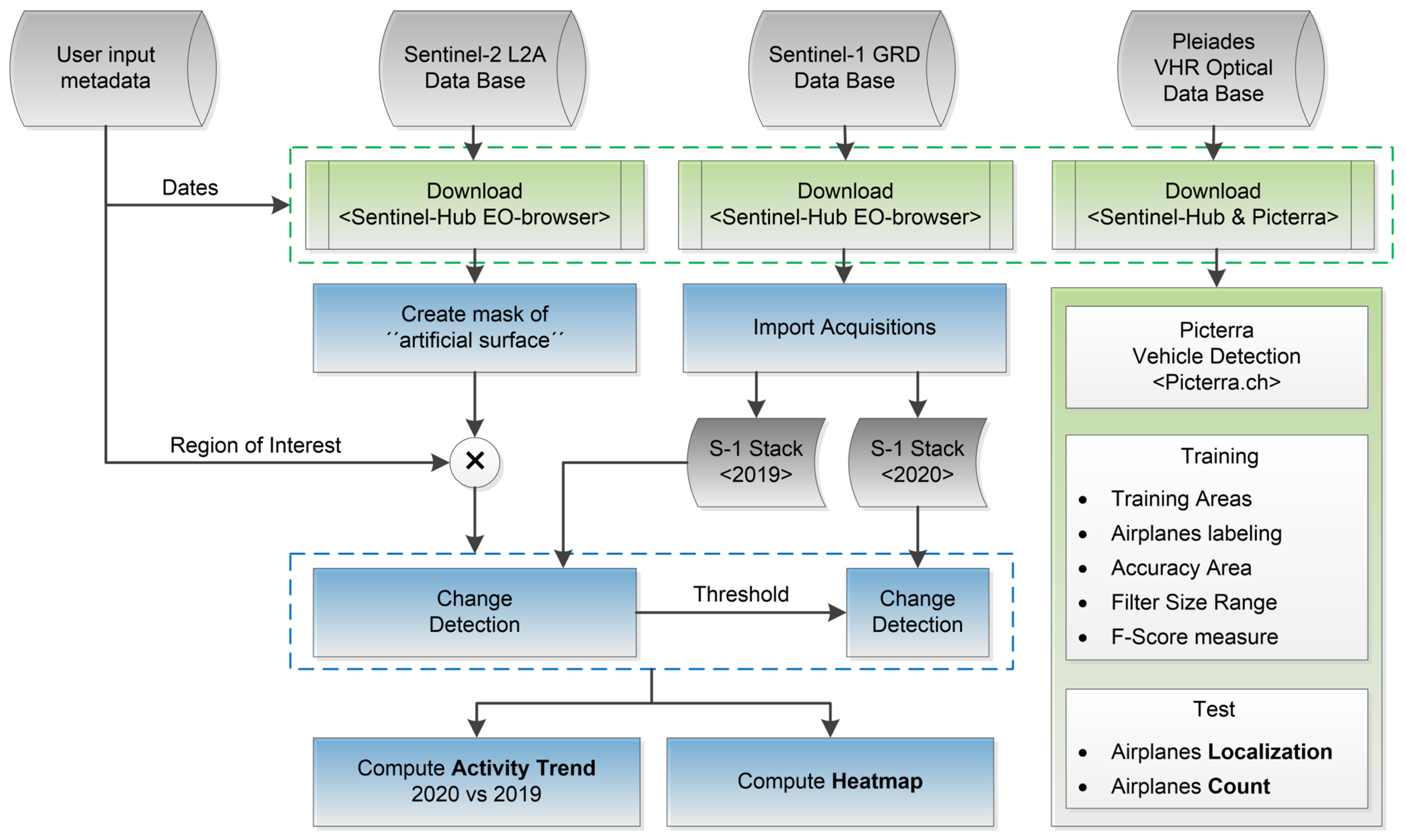
• Level-1 processing, which generates quantitative measurements of crucial variables on the selected target area, i.e., the artificial surface mask extracted from S-2 cloud-free acquisitions, the heat-map addressing to activity within the airport in a S-1 time-series, and, finally, the count and localization of the airplanes using Pleiades data.
• Level-2 processing, which generates SA insights by combining the results obtained at Level-1 with the external in situ measurements depicted in Figure 2b.

A graphical representation of the two processing levels is provided in Figure 4 and Figure 5, for Level-1 and Level-2, respectively.

In

Table 4. Pros (Y) and Cons (N) comparison table among HR Sentinel-1/-2 data, VHR Pleiades data, and their combination.

Property	HR Sentinel-1/-2 Data	VHR Pleiades Data	Combination
Constant repeat-pass coverage	Y	N	Y
(free-of-charge)
Frequent revisit time	Y	N	Y
(free-of-charge)
Direct data interpretation	N	Y	Y
(e.g., airplane detection/localization)
Sub-meter resolution	N	Y	Y

, we highlight Sentinel and VHR data’s advantages and limitations as we use them in the proposed algorithm.

3.1. Level-1 Processing

At this stage, we consider three different input sources: the HR data acquired by the S-1 and S-2 constellations and the VHR optical data of Pleiades. We aim to exploit the complementarity of all different sensors to extract quantitative measurements of selected critical features. Therefore, we can profitably use them at a later stage for SA applications (Level-2 processing). In the specific, we exploit SAR data from the S-1 constellation to obtain an indicator of the level of ongoing activity in a given observation time. S-1 time series is the ideal instrument for performing this kind of monitoring as they provide geocoded, detected SAR amplitude images, which are almost weather-independent, have a revisit time of only 6 days, and a favorable resolution of 10 m in azimuth and range dimensions [36].

S-2 data, instead, support the change detection algorithm by providing an up-to-date land cover map that we use for identifying man-made structures. The opportunity of having a land cover generated by independent data, with respect to the one used for change detection, enhances the activity level monitoring, as we explain in the following.

While Sentinel data provide average information about the ongoing activity level, we further need space- and time-tagged details on the airplane’s position to provide SA insights. For this purpose, we exploit the pair of VHR Pleiades data acquired just before and after Italy’s lockdown date. We use the object detection algorithm provided by the Picterra platform during the COVID-19 Custom Script Contest [37]. In this way, we have been able to correctly locate airplanes within a given airport area and on a specific date.

Finally, we correlate the Sentinel activity monitoring with this last information to provide advanced insights, as shown later in the Level-2 processing section.

In the following, we describe the single processing that we adopted for each of the exploited sensors. Figure 6 indicates the processing chain for the S-2, S-1, and Pleiades constellations with red, blue, and green colors, respectively.

Section 3.1.1 describes the steps for extracting the artificial surface mask by using S-2 cloud-free acquisitions, while Section 3.1.2 shows the technique used for detecting changes in a S-1 time-series. Finally, Section 3.1.3 introduces the vehicle detection algorithm provided by Picterra.

3.1.1. Artificial Surface Mapping from S-2 Data

We use Sentinel-2 data to generate an up-to-date map of artificial surfaces. In particular, we exploited the Normalized Difference Built-up Index (NDBI) to discard vegetated areas that could show unexpected temporal variations of the SAR backscatter due to scene changes as ground moisture fluctuations. Artificial surfaces usually show a stable backscatter, and by discarding vegetated areas, we can ascribe scene changes mainly to human operations. Specifically, the NDBI is defined as

$$NDBI=\frac{SWIR-NIR}{SWIR+NIR}$$

(1)

The Short-Wave Infrared (SWIR) band ranges between 1550 and 1750 nm, while the near-infrared (NIR) band falls roughly between 760 and 900 nm. As shown in Equation (1), this index can be used to identify urban areas where there is typically a higher reflectance in the SWIR band with respect to the NIR one. Even though the NDBI was originally developed for the Landsat Thematic Mapper (TM) bands 5 (SWIR) and 4 (NIR) [38], we replicated it using Sentinel-2 bands 11 (SWIR) and 8 (NIR) [39], by simply substituting these two bands to Equation (1):

$$NDBI=\frac{B11-B08}{B11+B08}$$

(2)

The artificial surface mask (ART) was then generated by considering the NDBI of 2019 and 2020. Therefore, the artificial surface mask, which may also include bare soil, was computed as

$$ART=(NDB{I}_{2020}>\lambda )·(NDB{I}_{2019}>\lambda )·RoI$$

(3)

The $RoI$ is the binary mask related to the Region of Interest that the user can define for a local investigation, while both the NDBI values are thresholded using a shared value, denoted as $\lambda$. We empirically set the value of the threshold to $\lambda =-0.15$. By applying this artificial surface mask, we link all the visible changes to the ones happening over the airport surface. This step contributes to automatizing the algorithm.

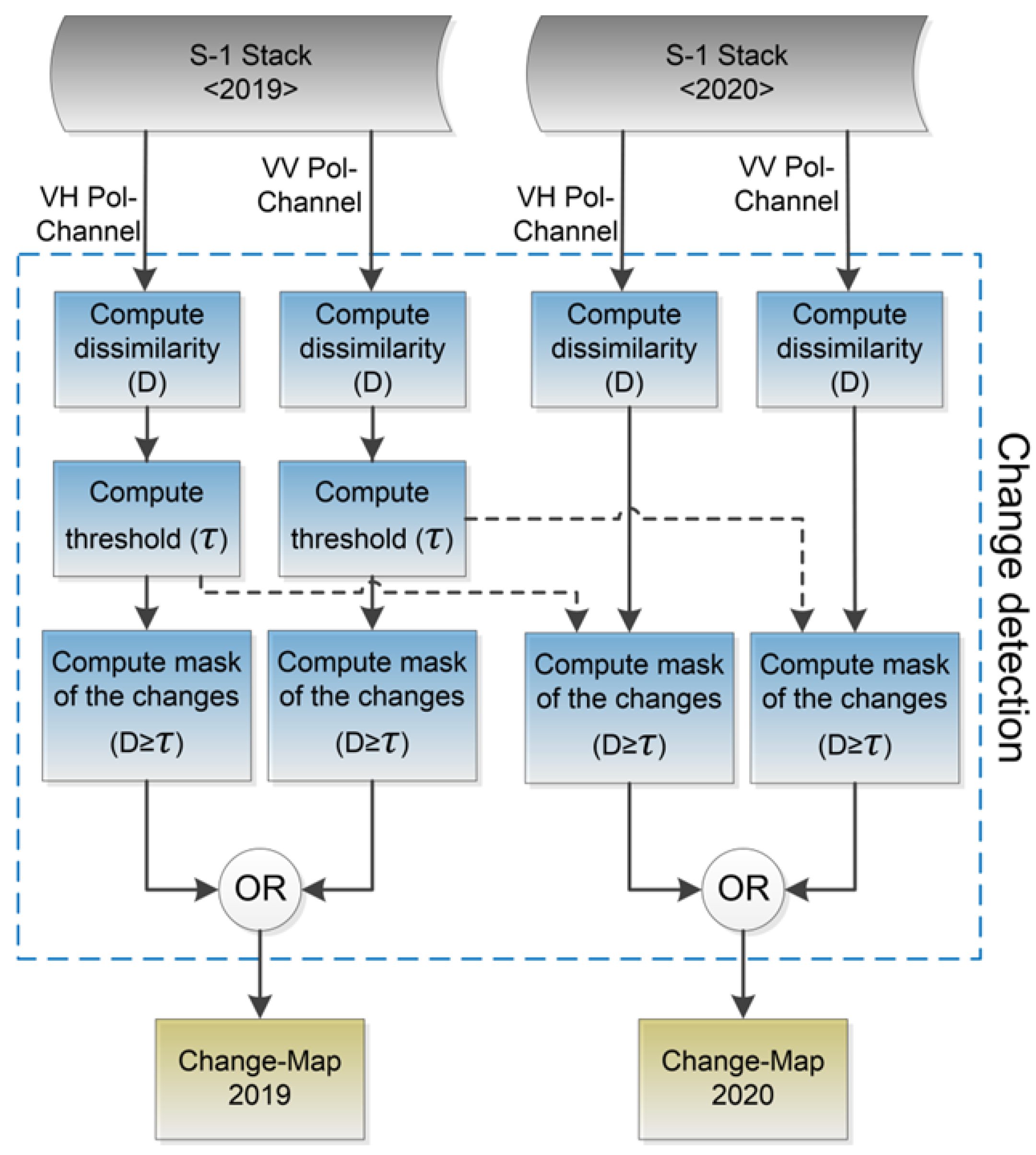
3.1.2. Activity Level Determination from S-1 Time Series

To provide the human activity level indicator, we import the temporal acquisition stack. We co-register all the N images to a master image, chosen as the most dated one in the stack. This preprocessing is needed since a possible spatial shift may happen in the data. Furthermore, it is possible that some data of the time-series are missing or are affected by bad weather conditions and therefore need to be discarded. In this work, we use all available data within the $RoI$ to identify the activity level indicator during the observation interval. We extract a set of N consecutive maps of changes, here indicated as changeMap. The algorithm’s block diagram is depicted in the blue polygon of Figure 6. In particular, we retrieve two products from the changeMap stack:

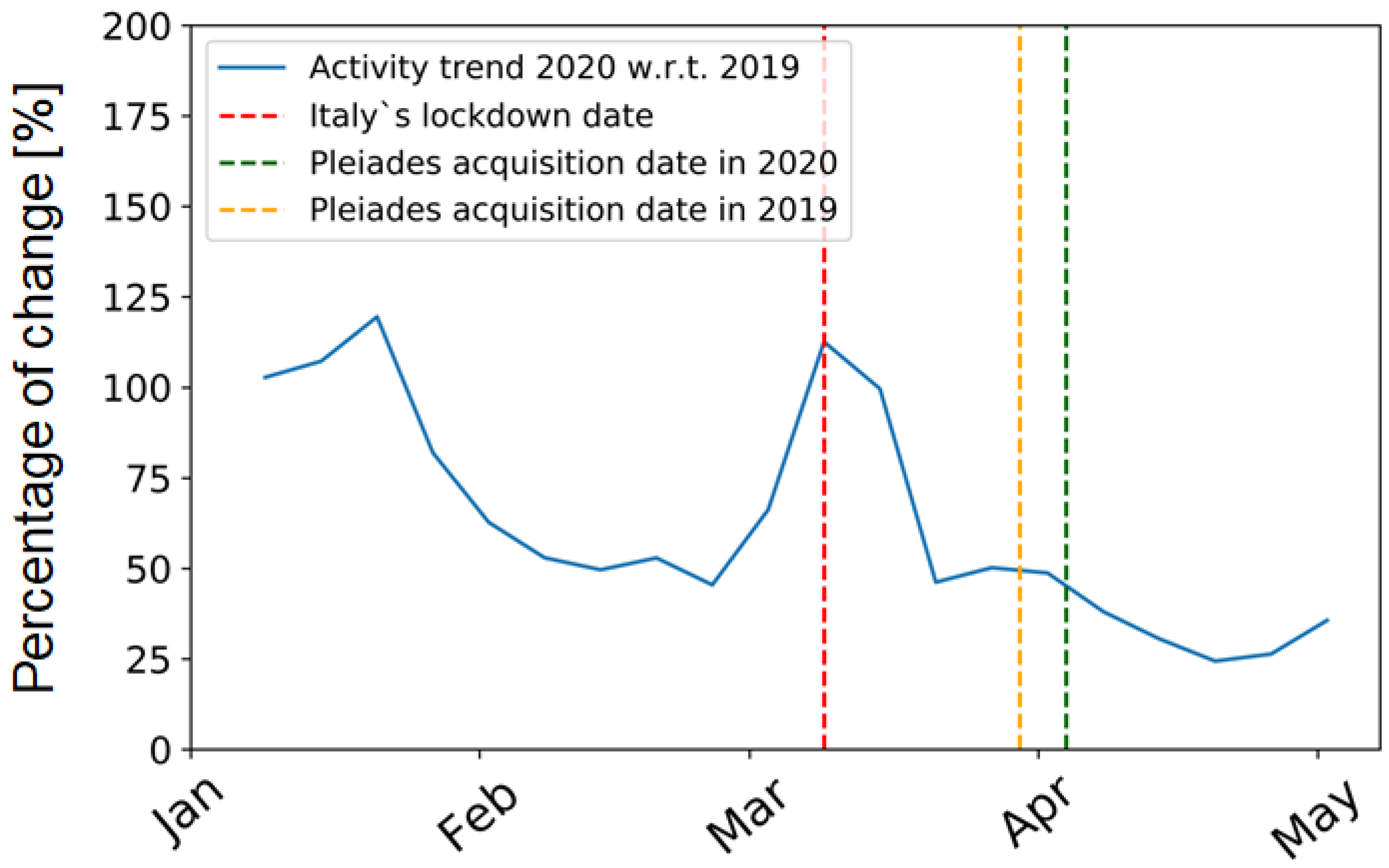
• Activity Trend: a plot showing the relative changes (in percentage) for the year 2020 with respect to 2019. It is computed as the ratio between the two temporal trends:

  $$\mathrm{activityTrend}=\frac{{\mathrm{trend}}_{2020}}{{\mathrm{trend}}_{2019}}·100$$

  (4)
  A percentage lower than 100% indicates higher activity in 2019, otherwise an exceed over the 100% points out the presence of more changes in 2020 than in 2019. In this work, we consider as a temporal trend, the evolution of the average of the change-map at each time instant.
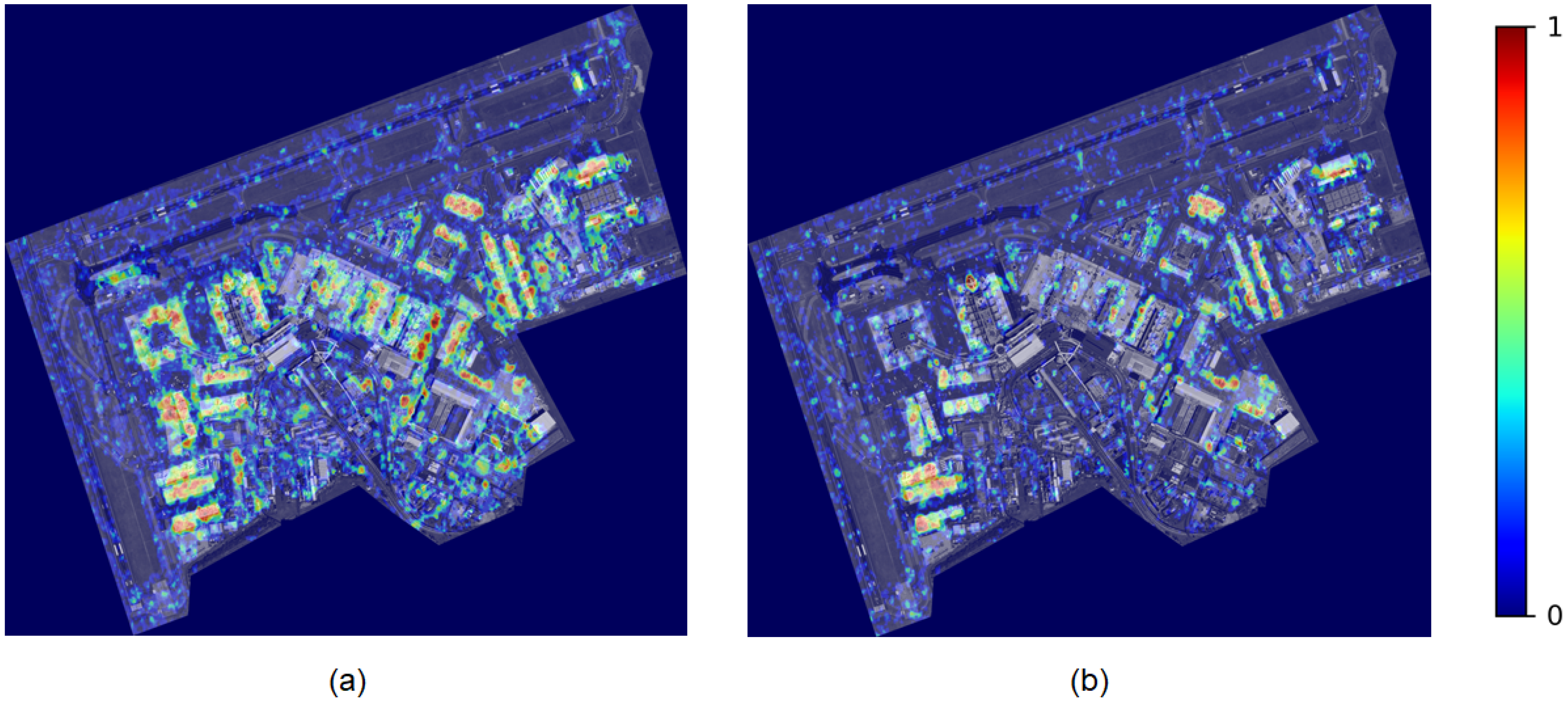
• Heat-Map: a digital map showing the degree of activity detected for each pixel during the whole observation time. We compute it as the temporal average of the change-map in a single pixel p:

  $$\mathrm{heatMap}=\frac{1}{N}\sum _{p=1}^N\mathrm{changeMap}\left(p\right)$$

  (5)

  where N is the number of changes within the time series. A pixel always detected as change along the time series corresponds to a $heatMap$ value equal to 1.

Figure 7 describes more in depth the change detection stage for the generation of the changeMap stack. In both the S-1 Stack 2019 and Stack 2020, we analyzed the change detection of only two consecutive images to preserve temporal resolution. A dissimilarity measure (D) based on speckle statistic is used for describing the changes in a scene. It is a statistical measurement used to define the dissimilarity between two SAR amplitude samples [40]:

$$D=\sum _{3\times 3}ln\left(\frac{x^2+y^2}{x·y}\right)$$

(6)

where x and y are SAR backscatter amplitude values, both corresponding to the same position p but acquired with a temporal baseline of 6 days, i.e., S-1A/B repeat pass. For the sake of simplicity, we indicate with $\sum _{3\times 3}(·)$ the moving average over a 3-by-3 pixels kernel. According to the work in [41], in this work, the dissimilarity measure is used for observing the changes within SAR multi-temporal stacks. In particular, a change is detected when the dissimilarity D is greater than a given threshold $\tau$, at least in one of the two available polarization channels:

$$D\ge \tau$$

(7)

The proposed algorithm is able to automatically set the threshold $\tau$. As we masked out all the vegetated areas using Sentinel-2 NDBI, as presented in Section 3.1.1, we assume that the computed dissimilarities can all be linked to changes in the airport. Therefore, we assume that a given percentage of the scene remains stationary, while the rest corresponds to actual changes. For this computation we consider the dissimilarity D computed over the whole stack. The threshold $\tau$ is therefore the value of dissimilarity $D_0$ for which the following condition holds,

$$\tau =D_0:{\int }_{D_0}^{D_{MAX}}hist\left(D\right)=\Delta$$

(8)

where $D_{MAX}$ is the maximum value of dissimilarity D over the whole stack, hist() is the normalized histogram of D, and $\Delta$ corresponds to actual changes.

As we cannot quantify the amount of change happening in a given scene in absolute terms, but this is a measure relative to the variation observed within the whole stack, we need to set the $\Delta$ parameter according to the user perception. Therefore, we define the $\Delta$ as a function of a meta-parameter called $sensitivity$:

$$\Delta =\frac{\mathrm{sensitivity}}{5}.$$

(9)

We define the $sensitivity$ between 0 and 1, and the user can intuitively set it without in-depth knowledge of the SAR system. This qualitative index allows the user to specify the amount of change that the algorithm should detect. Higher sensitivity levels (towards 1) increases the detection of small changes, while, on the contrary, lower sensitivity (towards 0) implies that the algorithm will identify only larger changes. We empirically examined different values for the sensitivity in this work, and we fixed it to 0.8.

The change detection from the Sentinel-1 time series is the core of the presented algorithm. It has the following fundamental properties.

• Spatial and temporal resolution preservation: we provide change maps with the same spatial and temporal resolution of Sentinel-1 Ground Range Detected (GRD) data, 10 m and 6 days for the spatial and temporal dimensions, respectively. In this way, it is possible not only to turn the level of ongoing activity on the overall observation period (the heat-map) upside down, but also to provide time-related variables, such as temporal activity dynamics (called the activity trend).
• Accuracy: by considering the statistics of detected SAR amplitudes, we can increase the detection accuracy by using a lower number of data. A statistical measure is used to define the dissimilarity between two SAR amplitude samples.
• Robustness: the algorithm is independent of the input SAR data and pre-processing. Indeed, it can process Single-Look Complex (SLC) data as multi-looked data with any number of looks with no change in the algorithm.
• Automatic: the algorithm automatically sets a threshold for the change detection. The user can define a level of sensitivity to detect even smaller changes (higher sensitivity) or identify only the largest ones (lower sensitivity).
• Comparable performance: the algorithm computes a unique threshold and applies it to other stacks with the same dimension. In this way, the algorithm can map similar activity levels into identical output values, e.g., the heat-map.

To obtain comparable results on different S-1 stacks, we used the same threshold for all stacks. We computed $\tau$ on Stack 2019 and applied it for Stack 2020.

Algorithm 1 shows the pseudocode related to the proposed SAR processing. The computational time for processing the two exploited SAR stacks is 185 s on an Intel(R) Xeon(R) CPU E5-2698 v4 @ 2.20 GHz.

Algorithm 1: Pseudocode for the generation of the activity trend and heat-maps from S-1 GRD temporal series acquisitions.

INPUT: Stack 2019 (VV, VH), Stack 2020 (VV, VH), ART (Equation 3), $sensitivity$ OUTPUT: Activity Trend, Heat-Map 2019, Heat-Map 2020 compute: dissimilarity measure D (Equation 6)       for each Year (2019, 2020) do             for each Polarization (VV, VH) do                   x := Stack, y := shift(Stack,1)                   compute: $D(x,y)$ (Equation 6)       return: $D_{2019}^{VV}$, $D_{2019}^{VH}$, $D_{2020}^{VV}$, $D_{2020}^{VH}$ compute: Threshold ${\tau }^{VV}$ for $D_{2019}^{VV}$ (Equation 8). compute: Threshold ${\tau }^{VH}$ for $D_{2019}^{VH}$ (Equation 8). compute: Change Map 2019       $changeMa{p}_{2019}$ := ((($D_{2019}^{VV}$ >= ${\tau }^{VV}$) or ($D_{2019}^{VH}$ >= ${\tau }^{VH}$)) and ART) compute: Change Map 2020       $changeMa{p}_{2020}$ := ((($D_{2020}^{VV}$ >= ${\tau }^{VV}$) or ($D_{2020}^{VH}$ >= ${\tau }^{VH}$)) and ART) compute: Trend for the year 2019       $tren{d}_{2019}$: average $changeMa{p}_{2019}$ at each acquisition time compute: Trend for the year 2020       $tren{d}_{2020}$: average $changeMa{p}_{2020}$ at each acquisition time compute: $activityTrend$ (Equation 4) compute: Heat-Maps for the year 2019       $heatMa{p}_{2019}$: average $changeMa{p}_{2019}$ along time dimension (Equation 5) compute: Heat-Maps for the year 2020       $heatMa{p}_{2020}$: average $changeMa{p}_{2020}$ along time dimension (Equation 5)

3.1.3. Airplane Detection

As mentioned in Section 2.4, we used Pleiades data for detecting airplanes in different areas of the Fiumicino airport and on different time-frames. This analysis allows for counting the number of aircraft in a given airport area, enabling the generation of results with a higher semantic. The dashed green rectangle in Figure 6 shows the methodology adopted for the extraction of two critical variables: the localization and count of airplanes within the airport, respectively.

The automatic detection of objects with arbitrary orientations and complex appearance has recently received increasing attention also in the remote sensing field [42]. At present, we can categorize the existing approaches in literature into two main branches:

• traditional machine learning methods based on varied computer vision techniques and
• deep learning techniques [43].

While the former needs feature extraction techniques, the latter is undoubtedly more attractive thanks to its low dependence on feature engineering and, not least, its improved performance on a large data scale. The high detection accuracy and the availability of pretrained DL models make this latter category a favorable choice for the present study. We distinguish between two main DL approaches: the Region-based Convolutional Neural Network (R-CNN) and the You Only Look Once (YOLO) models.

The former approach considers three steps:

• find regions in the image that might contain an object,
• extract CNN features from these regions, and, finally,
• classify the objects using the extracted features.

For this category, three variants have been developed at present. Indeed, the algorithm proposed initially in R-CNN [44], has been modified to speed up the processing of these three steps in the Fast R-CNN [45] and the Faster R-CNN [46].

The latter category applies a single neural network to the full image (from this the name “you only look once”) and divide it into regions. For each of them, the algorithm predicts bounding boxes, which are then weighted by pretrained probabilities [47]. This family of algorithms is nowadays really popular because it achieves high accuracy while also running in real-time applications. Improvements to the first version of YOLO [47] of 2016 are steadily coming up on a yearly basis, as the YOLOv2 [48] of 2017 and the YOLOv3 [49] of 2018.

In the present work, we relied on the software provided by the Swiss company Picterra [37]. This platform enables the user to train Deep Learning models to automatize objects’ detection with geospatial imagery. Picterra uses a modified version of the Mask R-CNN [50], an architecture designed to object instance segmentation, which combines the results of two branches: the former uses the Faster R-CNN for bounding box recognition. At the same time, the latter predicts an object mask.

Without any programming requirements, it is possible to train and build a custom detector using human-made annotations and the Picterra GPU-enabled infrastructure. In the performed analysis, we first created a training data set by labeling a list of airplanes on Pleiades imagery, presented in Figure 3. This visual selection has been performed manually, thanks to the Picterra graphic interface (see Figure 8). Second, we validated the performances of the detector on dedicated areas, highlighted with red boxes in Figure 3. Finally, we tested the modified Mask R-CNN algorithm on the two Pleiades acquisitions available over the Fiumicino Airport in 2019 and 2020.

As a performance parameter of the trained detector, we used the F1-Score. In a binary classification problem, a confusion matrix C is a 2-by-2 array that summarizes the results of testing the classifier for further inspection:

$$C=\left[\begin{array}{cc}TP& FN\\ FP& TN\end{array}\right],$$

(10)

where the four outcomes report the number of $TP$ (true positives), i.e., the inputs correctly predicted by the model; $TN$ (true negatives), i.e., the ones correctly rejected by the model; $FN$ (false negatives), i.e., the missed positives; and $FP$ (false positives), i.e., the false alarms. To get an understanding and measure of relevance from the confusion matrix it is possible to extract the precision (P):

$$P=\frac{TP}{TP+FP},$$

(11)

and the recall (R):

$$R=\frac{TP}{TP+FN}.$$

(12)

The precision determines the costs of false alarms (false positives, $FP$). At the same time, recall calculates how many of the actual positives the model captures by labeling it positive (true positives, $TP$). F1-Score ($F1$) is needed for balancing between precision and recall, and it is defined as

$$F1=\frac{2·P·R}{P+R}.$$

(13)

It is the harmonic mean of precision and recall and considers both false positives and false negatives. It reaches its best value at $100\%$ when both precision and recall equals $100\%$.

Among the detector settings, Picterra allows the user to insert a filter size parameter, which sets a constraint on the target object’s minimum and maximum size (in square meters). We set these parameters as the one that allows achieving the best F1-score. There we obtain a filter size as $min=60$ m${}^2$ and $max=1400$ m${}^2$, and a detector with a precision of $88.89\%$ and a recall of $99.92\%$, which correspond to an F1-Score of $94.08\%$.

3.2. Level-2 Processing

Although the output obtained from the Level-1 processing brings already very insightful outcomes about the ongoing activity over the airport, we further aggregate these results in a Level-2 processing procedure, obtaining enhanced semantic results, which enable Situational Awareness. Given the output derived from the multi-sensor system described in Section 3.1, we provide SA insights by combining the HR and VHR outputs with the external in situ measurements described in Section 2.1. The Level-2 processing chain is depicted in Figure 5. It consists of correlating the activity level indicator with the airplane localization and counting for the single specific areas of interest within the airport ecosystem. The latter are created through a series of masks as described in Section 2.1 and are depicted in Figure 2.

By mixing the information of the heat-map with the localization and count of the airplanes on a given date, we extracted information about the airport operability and the usage of different airport areas after the lockdown of Spring 2020, as we show in the following section.

Although the present analysis aims only at demonstrating the potential of this approach and provides a user-defined threshold setting, the proposed methodology could also be automatized, given the availability of a more extensive VHR data set.

4. Results and Discussion

In the following, we present the experimental results obtained for the considered test case scenario. In particular,

• we concentrate on the system performance assessment by comparing the airport activities of the Stack 2020 with the Stack 2019, described in Table 1;
• analyze within the sole Stack 2020 the activity levels detected over the airport before and after Italy’s Spring lockdown, officially imposed on 9 March 2020; and
• extend the analysis to airplane detection with Pleiades VHR data, using the methodology described in Section 3.1.3.

4.1. Airport Activity Levels

As for the first proposed analysis, we compare the airport’s ongoing activity levels in 2019 and 2020. We show the results as normalized heat-maps, which assume values between 0 (no change detected) and 1 (change always detected). Figure 9 shows the heat-maps retrieved by applying the proposed algorithm. As expected, we notice a clear activity level fall-off during 2020 with respect to the previous year. Indeed, in Figure 9, the heat-map in 2020 (b) appears much less bright if compared to the corresponding 2019 one in (a).

In particular, we observe a drastic activity reduction over the apron areas directly connected with the terminal buildings. At the same time, we detect a less severe change in the rest of the airport’s areas. Furthermore, as expected, we also observe how the activities over the taxi-ways, i.e., those paths for aircraft connecting runways with aprons, hangars, terminals, and other facilities, considerably decreased in 2020 with respect to 2019. In Figure 10, we show a detail of the apron areas. We notice that we can detect activity levels for the single gate, as visible in the image’s top-right corner.

Alternatively, we perform additional analysis of airport activity levels by observing the trends computed as explained in Section 3.1.2 and showed in Figure 11. We indicate this quantity as the percentage activity trend in the year 2020 with respect to the one in 2019. As shown in Figure 11, we observe a monotonic decreasing trend just after the lockdown event on 9 March 2020, which is marked in the figure with a dashed red vertical line. The yellow and green lines indicate the acquisition dates of the Pleiades data in 2019 and 2020, respectively. We also notice a decreasing trend before the lockdown period. This event is probably due to a general decrease in the flights during the Chinese COVID-19 lockdown, already started in January 2020 [51].

4.2. Airport Activity Levels before and after the Lockdown Event

To complete our analysis on activity levels and sustain the observed decreasing trend measured after the COVID-19 lockdown with additional results, we also compare the activity levels before and after the lockdown event. Figure 12 presents the heat-maps (a) before and (b) after 9 March 2020.

We split the Stack 2020 in two and applied the algorithm explained in Section 3.1.2 to compute the activity level on half of the stack.

By using this approach, we provide more detailed information about the lockdown consequences of airport activities. Here, we notice a severe reduction of the activities after the lockdown in subfigure (b) with respect to the activity map before the lockdown (a). Moreover, we can also notice other patterns for airport activity levels. Indeed, the main activities are transferred to areas far away from the terminals.

Compared with Figure 10b, Figure 13b better highlights the measure of activity centralization to a few gates adopted in the airport. Furthermore, Figure 13b shows on its left-hand side the closure of an entire boarding area during the lockdown.

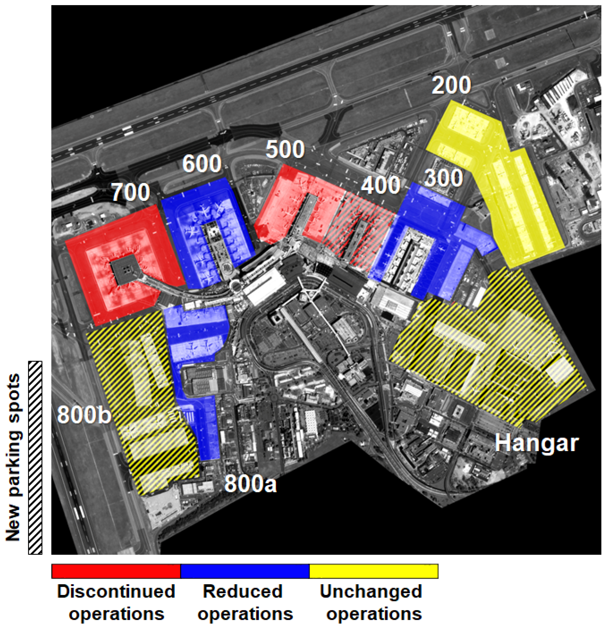
4.3. Airplanes Detection and Situational Awareness

As part of the proposed methodology, we exploit Very-High-Resolution optical images from the Pleiades constellation to detect airplane numbers and their position over the airport area. We perform the detection within the blue box marked in Figure 14, which also shows the airplanes identified over the images. Although the total number of airplanes counted in the blue rectangles is almost the same in both the images, we can obtain useful insights from this result by considering the airplane position and linking it to the one derived from the activity levels. Furthermore, we also notice that in subfigure (b) of Figure 14 there is no aircraft presence on the taxi-ways, which is usually dedicated to maneuvers before and after the flight, while it is present in subfigure (a). Eventually, we also notice a higher concentration of airplanes in the hangar in 2020, with respect to 2019, confirming that most of the fleets were grounded at the time.

The comparison in Figure 14 confirms the need for semantic SA results to describe better the effect of the lockdown and the activity change in the airport. Indeed, we cannot assume any change in the airport area management from the simple airplane localization and count. For this reason, we need to aggregate the results obtained from the Sentinels and Pleiades constellations together. In the following, we show the results obtained by applying the Level-2 processing, as explained in Section 3.2. In the specific, we consider the masks of Figure 2 and described in Section 2.1, to correlate activity levels and airplane count for each selected airport areas.

We report these new results in Figure 15 in the form of bar-plots and scatter-plots. For the 2019 (green bars) and the 2020 (red bars), we first compare the number of airplanes and the average heat-map values within each airport area in Figure 15a and Figure 15b, respectively. Second, we plot the number of airplanes versus the average heat-map values within each given area for 2019 and 2020, in Figure 15c and Figure 15d, respectively.

From the obtained results, we can affirm that aggregated outputs provide unique and insightful clues, that are way more informative with respect to one obtainable from the single satellite product.

By observing together the plots of Figure 15, we propose a non-expert interpretation about the area usage for each of the analyzed areas after the 2020’s lockdown:

• Hangar: has kept its functionality of airplane parking spot, hosting a higher number of airplanes during the lockdown, with respect to the previous year;
• 200: is probably one of the few areas which kept its full functionality as terminal and service area also during the lockdown;
• 300: decreased activity, but same functionality;
• 400: the increased number of airplanes together with the reduction of the average activity suggest that this area has been closed and used as parking area. This area corresponds indeed to Terminal 1, which was closed on the 17 March 2020 [33];
• 500: the strong decrease in average activity and number of airplanes suggests that this terminal area was closed;
• 600: kept its functionality, but probably only one gate was kept open as the red spot is indicating in Figure 13b;
• 700: as for the 500, this area shows a drastic decrease in both average activity and number of airplanes, suggesting that this terminal was closed;
• 800a: decreased activity, but same functionality;
• 800b: similar to area 200, this area probably kept its functionality. Since it showed a large number of airplanes and a low average activity, we can assume that it was also used as parking spot.

Finally, the combination of the results facilitates the generation of high-level semantic maps. As end-product we propose the map depicted in Figure 16. In this map we identify areas usage as

• discontinued operations (red): areas with low average activity and low number of airplanes;
• reduced operations (blue): regions with lower average activity w.r.t. 2019 and same number of airplanes w.r.t 2019;
• unchanged operations (yellow): spots presenting high average activity and high number of airplanes; and
• new parking spots (with stripes): areas with low average activity and high number of grounded airplanes.

This new information can be used to plan for the safe reopening of the airport after the lockdown period, managing the various terminals and gates as efficiently as possible.

5. Conclusions

This work demonstrates the potential of existing Remote Sensing constellations for Situational Awareness applications. Our approach can effectively support the remote sensing analyst’s decision-making process to bridge the gap between data and underlying insights. This methodology can be integrated into existing SA systems, such as the recent RACE—Rapid Action on Coronavirus and EO—platform, which aggregates satellite data from the different Copernicus constellations, to provide up-to-date natural and economic indicators. In the proposed test case, we showed how we exploit the derived activity levels from Sentinel-1 time-series as a crucial variable for monitoring the Rome Fiumicino airport operability. Additionally, we showed the aggregation of these results with the aircraft count and localization for different airport areas to provide high-semantic products about the airport surface utilization. Finally, the proposed methodology sets the groundwork for future applications, which will benefit from the availability of higher spatial and temporal resolution data sets. Indeed, while SA methodologies based on RS data are nowadays only a small percentage of SA applications, in the future, these are foreseen to spread out and serve different natural and economic sectors.

As a future activity, we aim at further extending the proposed methodology by exploiting Sentinel-1 interferometric capability and use the coherence parameter as an additional input feature. The S-1 interferometric coherence can be indeed used for finer change detection and to perform land cover classification as in [52], together with the application of deep learning approaches [53].

Future investigations will also include applying the proposed methodology to other infrastructures, such as commercial harbors, stadiums, and tourist places. Furthermore, we could extend the analysis to other airport areas and other variables, e.g., car parking spots or vehicle activities in the cargo areas. Analogously, we could also investigate correlations with in situ variables, e.g., the number of passengers and cargo flights. Eventually, we aim to automatize the level-2 processing, i.e., determine new areas operability. Indeed, with a broader number of available VHR Pleiades images, it would be possible to correlate the retrieved indexes to areas’ operability automatically.

References

1. Endsley, M. Design and evaluation for situational awareness enhancement. In Proceedings of the Human Factors Society 32nd Annual Meeting, Anaheim, CA, USA, 24–28 October 1988; pp. 97–101. [Google Scholar]
2. Smith, K.; Hancock, P.A. Situation Awareness Is Adaptive, Externally Directed Consciousness. Hum. Factors 1995, 37, 137–148. [Google Scholar] [CrossRef]
3. Adams, M.J.; Tenney, Y.J.; Pew, R.W. Situation Awareness and the Cognitive Management of Complex Systems. Hum. Factors 1995, 37, 85–104. [Google Scholar] [CrossRef]
4. Jensen, R.S. The Boundaries of Aviation Psychology, Human Factors, Aeronautical Decision Making, Situation Awareness, and Crew Resource Management. Int. J. Aviat. Psychol. 1997, 7, 259–267. [Google Scholar] [CrossRef]
5. Li, W.C. The casual factors of aviation accidents related to decision errors in the cockpit by system approach. J. Aeronaut. Astronaut. Aviat. 2011, 43, 147–154. [Google Scholar]
6. D’Arcy, J.; Della Rocco, P.S. Air traffic control specialist decision making and strategic planning—A field survey. In Technical Report DOT/FAA/CT-TN01/05; U.S. Department of Transportation, Federal Aviation Administration: Washington, DC, USA, 2001. [Google Scholar]
7. Kalluri, S.; Gilruth, P.; Bergman, R. The potential of remote sensing data for decision makers at the state, local and tribal level: Experiences from NASA’s Synergy program. Environ. Sci. Policy 2003, 6, 487–500. [Google Scholar] [CrossRef]
8. King, R.L. Putting Information into the Service of Decision Making: The Role of Remote Sensing Analysis. In Proceedings of the IEEE Workshop on Advances in Techniques for Analysis of Remotely Sensed Data, Greenbelt, MD, USA, 27–28 October 2003; pp. 25–29. [Google Scholar]
9. Roemer, H.; Kiefl, R.; Henkel, F.; Cao, W.; Nippold, R.; Kurz, F.; Kippnich, U. Using Airborne Remote Sensing to Increase Situational Awareness in Civil Protection and Humanitarian Relief—The Importance of User Involvement. In Proceedings of the International Archives of the Photogrammetry, Remote Sensing and Spatial Information Sciences, Prague, Czechia, 12–19 July 2016; Volume XLI-B8, pp. 1363–1370. [Google Scholar]
10. Borowitz, M. Strategic Implications of the Proliferation of Space Situational Awareness Technology and Information: Lessons Learned from the Remote Sensing Sector. Space Policy 2018, 47, 18–27. [Google Scholar] [CrossRef]
11. Schroeter, E.; Kiefl, R.; Neidhardt, E.; Gurczik, G.; Dalaff, C.; Lechner, K. Trialing Innovative Technologies in Crisis Management—“Airborne and Terrestrial Situational Awareness” as Support Tool in Flood Response. Appl. Sci. 2020, 10, 3743. [Google Scholar] [CrossRef]
12. Boschetti, L.; Roy, D.P.; Justice, C.O. Using NASA’s World Wind virtual globe for interactive internet visualization of the global MODIS burned area product. Int. J. Remote Sens. 2008, 29, 3067–3072. [Google Scholar] [CrossRef]
13. The Guardian. Coronavirus Will Reshape Our Cities—We Just Don’t Know How Yet. 2020. Available online: https://www.theguardian.com/world/2020/may/22/coronavirus-will-reshape-our-cities-we-just-dont-know-how-yet (accessed on 14 October 2020).
14. PWC. Five Actions Can Help Mitigate Risks to Infrastructure Projects Amid COVID-19. 2020. Available online: https://www.pwc.com/gx/en/industries/capital-projects-infrastructure/publications/infrastructure-covid-19.html (accessed on 14 October 2020).
15. World Bank. COVID-19 and Infrastructure: A Very Tricky Opportunity. 2020. Available online: https://blogs.worldbank.org/ppps/covid-19-and-infrastructure-very-tricky-opportunity (accessed on 14 October 2020).
16. McKinsey & Co. A New Paradigm for Project Planning. 2020. Available online: https://www.mckinsey.com/industries/capital-projects-and-infrastructure/our-insights/a-new-paradigm-for-project-planning (accessed on 14 October 2020).
17. Zhang, Z.; Arshad, A.; Zhang, C.; Hussain, S.; Li, W. Unprecedented Temporary Reduction in Global Air Pollution Associated with COVID-19 Forced Confinement: A Continental and City Scale Analysis. Remote Sens. 2020, 12, 2420. [Google Scholar] [CrossRef]
18. Zhang, K.; de Leeuw, G.; Yang, Z.; Chen, X.; Jiao, J. The Impacts of the COVID-19 Lockdown on Air Quality in the Guanzhong Basin, China. Remote Sens. 2020, 12, 3042. [Google Scholar] [CrossRef]
19. Nichol, J.; Bilal, M.; Ali, M.; Qiu, Z. Air Pollution Scenario over China during COVID-19. Remote Sens. 2020, 12, 2100. [Google Scholar] [CrossRef]
20. Fan, C.; Li, Y.; Guang, J.; Li, Z.; Elnashar, A.; Allam, M.; de Leeuw, G. The Impact of the Control Measures during the COVID-19 Outbreak on Air Pollution in China. Remote Sens. 2020, 12, 1613. [Google Scholar] [CrossRef]
21. Veefkind, J.; Aben, I.; McMullan, K.; Förster, H.; de Vries, J.; Otter, G.; Claas, J.; Eskes, H.; de Haan, J.; Kleipool, Q.; et al. TROPOMI on the ESA Sentinel-5 Precursor: A GMES mission for global observations of the atmospheric composition for climate, air quality and ozone layer applications. Remote Sens. Environ. 2012, 120, 70–83. [Google Scholar] [CrossRef]
22. Justice, C.O.; Vermote, E.; Townshend, J.R.G.; Defries, R.; Roy, D.P.; Hall, D.K.; Salomonson, V.V.; Privette, J.L.; Riggs, G.; Strahler, A.; et al. The Moderate Resolution Imaging Spectroradiometer (MODIS): Land remote sensing for global change research. IEEE Trans. Geosci. Remote Sens. 1998, 36, 1228–1249. [Google Scholar] [CrossRef] [Green Version]
23. Griffin, D.; McLinden, C.; Racine, J.; Moran, M.; Fioletov, V.; Pavlovic, R.; Mashayekhi, R.; Zhao, X.; Eskes, H. Assessing the Impact of Corona-Virus-19 on Nitrogen Dioxide Levels over Southern Ontario, Canada. Remote Sens. 2020, 12, 4112. [Google Scholar] [CrossRef]
24. Vîrghileanu, D.; Săvulescu, I.; Mihai, B.A.; Nistor, C.; Dobre, R. Nitrogen Dioxide (NO2) Pollution Monitoring with Sentinel-5P Satellite Imagery over Europe during the Coronavirus Pandemic Outbreak. Remote Sens. 2020, 12, 3575. [Google Scholar] [CrossRef]
25. Jechow, A.; Hölker, F. Evidence That Reduced Air and Road Traffic Decreased Artificial Night-Time Skyglow during COVID-19 Lockdown in Berlin, Germany. Remote Sens. 2020, 12, 3412. [Google Scholar] [CrossRef]
26. Elvidge, C.; Ghosh, T.; Hsu, F.C.; Zhizhin, M.; Bazilian, M. The Dimming of Lights in China during the COVID-19 Pandemic. Remote Sens. 2020, 12, 2851. [Google Scholar] [CrossRef]
27. Niroumand-Jadidi, M.; Bovolo, F.; Bruzzone, L.; Gege, P. Physics-based Bathymetry and Water Quality Retrieval Using PlanetScope Imagery: Impacts of 2020 COVID-19 Lockdown and 2019 Extreme Flood in the Venice Lagoon. Remote Sens. 2020, 12, 2381. [Google Scholar] [CrossRef]
28. Straka, W., III; Kondragunta, S.; Wei, Z.; Zhang, H.; Miller, S.; Watts, A. Examining the Economic and Environmental Impacts of COVID-19 Using Earth Observation Data. Remote Sens. 2021, 13, 5. [Google Scholar] [CrossRef]
29. Liu, Q.; Sha, D.; Liu, W.; Houser, P.; Zhang, L.; Hou, R.; Lan, H.; Flynn, C.; Lu, M.; Hu, T.; et al. Spatiotemporal Patterns of COVID-19 Impact on Human Activities and Environment in Mainland China Using Nighttime Light and Air Quality Data. Remote Sens. 2020, 12, 1576. [Google Scholar] [CrossRef]
30. Tanveer, H.; Balz, T.; Cigna, F.; Tapete, D. Monitoring 2011–2020 Traffic Patterns in Wuhan (China) with COSMO-SkyMed SAR, Amidst the 7th CISM Military World Games and COVID-19 Outbreak. Remote Sens. 2019, 12, 1636. [Google Scholar] [CrossRef]
31. European Space Agency (ESA). RACE: Rapid Action on Coronavirus and EO. 2020. Available online: https://race.esa.int/ (accessed on 28 December 2020).
32. Sentinel-Hub. COVID-19 Custom Script Contest by Euro Data Cube. 2020. Available online: https://www.sentinel-hub.com/develop/community/contest-covid/ (accessed on 28 December 2020).
33. Aeroporti di Roma (ADR). News 2020.03.17. Downsize Airport Operations. 2020. Available online: http://www.adr.it/de/web/aeroporti-di-roma-en-/viewer?p_p_id=3_WAR_newsportlet&p_p_lifecycle=0&p_p_state=normal&p_p_mode=view&p_p_col_id=column-2&p_p_col_pos=1&p_p_col_count=2&_3_WAR_newsportlet_jspPage=/html/news/details.jsp&_3_WAR_newsportlet_nid=18829902&_3_WAR_newsportlet_redirect=/de/web/aeroporti-di-roma-en-/azn-news (accessed on 14 October 2020).
34. Aeroporti di Roma (ADR). Aggiornamento Tariffario 2017—2021, Consultazioni con L’utenza: Investimenti. 2016. Available online: https://www.adr.it/documents/10157/9522121/2017-21+Investimenti+-+Incontro+Utenti+2016+__+v9+settembre.pdf/211fe00b-2b13-447d-afd9-dc0e49daa908 (accessed on 14 October 2020).
35. Gleyzes, M.A.; Perret, L.; Kubik, P. Pleiades System Architecture and main Performances. Int. Arch. Photogramm. Remote. Sens. Spat. Inf. Sci. 2012, XXXIX-B1, 537–542. [Google Scholar] [CrossRef] [Green Version]
36. Torres, R.; Snoeij, P.; Geudtner, D.; Bibby, D.; Davidson, M.; Attema, E.; Potin, P.; Rommen, B.; Floury, N.; Brown, M.; et al. GMES Sentinel-1 mission. Remote Sens. Environ. 2012, 120, 9–24. [Google Scholar] [CrossRef]
37. Picterra. Picterra—Geospatial Imagery Analysis Made Easy. 2018. Available online: https://picterra.ch (accessed on 14 October 2020).
38. Zha, Y.; Gao, J.; Ni, S. Use of Normalized Difference Built-Up Index in Automatically Mapping Urban Areas from TM Imagery. Int. J. Remote Sens. 2003, 24, 583–594. [Google Scholar] [CrossRef]
39. Drusch, M.; Bello, U.D.; Carlier, S.; Colin, O.; Fernandez, V.; Gascon, F.; Hoersch, B.; Isola, C.; Laberinti, P.; Martimort, P.; et al. Sentinel-2: ESA’s Optical High-Resolution Mission for GMES Operational Services. Remote Sens. Environ. 2012, 120, 25–36. [Google Scholar] [CrossRef]
40. Deledalle, C.A.; Denis, L.; Tupin, F. How to compare noisy patches? Patch similarity beyond Gaussian noise. Int. J. Comput. Vis. 2012, 99, 86–102. [Google Scholar] [CrossRef] [Green Version]
41. Sica, F.; Reale, D.; Poggi, G.; Verdoliva, L.; Fornaro, G. Nonlocal adaptive multilooking in SAR multipass differential interferometry. IEEE J. Sel. Top. Appl. Earth Obs. Remote Sens. 2015, 8, 1727–1742. [Google Scholar] [CrossRef] [Green Version]
42. Cheng, G.; Han, J. A Survey on Object Detection in Optical Remote Sensing Images. ISPRS J. Photogramm. Remote Sens. 2016, 117, 11–28. [Google Scholar] [CrossRef] [Green Version]
43. Zou, X. A Review of Object Detection Techniques. In Proceedings of the 2019 International Conference on Smart Grid and Electrical Automation (ICSGEA), Xiangtan, China, 10–11 August 2019; pp. 251–254. [Google Scholar]
44. Girshick, R.; Donahue, J.; Darrell, T.; Malik, J. Rich Feature Hierarchies for Accurate Object Detection and Semantic Segmentation. In Proceedings of the 2014 IEEE Conference on Computer Vision and Pattern Recognition, Columbus, OH, USA, 24–27 June 2014; pp. 580–587. [Google Scholar]
45. Girshick, R. Fast R-CNN. In Proceedings of the 2015 IEEE International Conference on Computer Vision (ICCV), Boston, MA, USA, 7–12 June 2015; pp. 1440–1448. [Google Scholar]
46. Ren, S.; He, K.; Girshick, R.; Sun, J. Faster R-CNN: Towards Real-Time Object Detection with Region Proposal Networks. IEEE Trans. Pattern Anal. Mach. Intell. 2017, 39, 1137–1149. [Google Scholar] [CrossRef] [Green Version]
47. Redmon, J.; Divvala, S.; Girshick, R.; Farhadi, A. You Only Look Once: Unified, Real-Time Object Detection. In Proceedings of the 2016 IEEE Conference on Computer Vision and Pattern Recognition (CVPR), Las Vegas, NV, USA, 27–30 June 2016; pp. 779–788. [Google Scholar]
48. Redmon, J.; Farhadi, A. YOLO9000: Better, Faster, Stronger. In Proceedings of the 2017 IEEE Conference on Computer Vision and Pattern Recognition (CVPR), Honolulu, HI, USA, 21–26 June 2017; pp. 6517–6525. [Google Scholar]
49. Redmon, J.; Farhadi, A. YOLOv3: An Incremental Improvement. arXiv 2018, arXiv:1804.02767. [Google Scholar]
50. He, K.; Gkioxari, G.; Dollár, P.; Girshick, R. Mask R-CNN. IEEE Trans. Pattern Anal. Mach. Intell. 2020, 42, 386–397. [Google Scholar] [CrossRef] [PubMed]
51. BBC. Coronavirus: What Did China Do about Early Outbreak? 2020. Available online: https://www.bbc.com/news/world-52573137 (accessed on 14 October 2020).
52. Sica, F.; Pulella, A.; Nannini, M.; Pinheiro, M.; Rizzoli, P. Repeat-pass SAR Interferometry for Land Cover Classification: A Methodology using Sentinel-1 Short-Time-Series. Remote Sens. Environ. 2019, 232, 111277. [Google Scholar] [CrossRef]
53. Mazza, A.; Sica, F.; Rizzoli, P.; Scarpa, G. TanDEM-X Forest Mapping Using Convolutional Neural Networks. Remote Sens. 2019, 11, 2980. [Google Scholar] [CrossRef] [Green Version]
Figure 1. Rome–Fiumicino International Airport: (a) Google Earth view of the analyzed area and (b) geocoded masks superimposed to Pleiades image.
Remotesensing 13 00299 g001
Figure 2. Site maps: (a) Apron areas defined in Aeroporti di Roma (ADR) official documents [34]. (b) Geocoded masks comprising the apron and hangar areas and superimposed to Pleiades image.
Remotesensing 13 00299 g002
Figure 3. VHR Pleiades images used for training and validation over the areas of (a,b) Zaventem—Brussels National Airport on 1 April 2019 and 18 March 2020, respectively; (c) Genoa—Christopher Columbus Airport on 30 April 2019; (d) Munich—Franz Josef Strauss International Airport on 4 April 2020; (e,f) south-eastern side of Madrid—Adolfo Suarez Barajas International Airport on 27 April 2019 and 28 March 2020, respectively; (g) Taipei—Songshan International Airport on 25 March 2020. The image crops marked in red in subfigures (b,d) are used for the validation only.
Remotesensing 13 00299 g003
Figure 4. Flowchart of Level-1 processing for multi-sensor variables retrieval.
Remotesensing 13 00299 g004
Figure 5. Flowchart of Level-2 processing for Situational Awareness insights’ generation.
Remotesensing 13 00299 g005
Figure 6. Flowchart of Figure 4 with superimposed three dashed polygons indicating the block diagrams for (Red) artificial surface mapping using S-2 data, (Blue) activity level determination using S-1 time series, and (Green) airplanes detection and localization on Pleiades acquisitions.
Remotesensing 13 00299 g006
Figure 7. Flowchart detail of the blue block in Figure 6: change detection algorithm adopted in the Sentinel-1 processing chain.
Remotesensing 13 00299 g007
Figure 8. Picterra platform graphic Interface screenshot.
Remotesensing 13 00299 g008
Figure 9. Comparison between heat-maps in 2019 and 2020: (a) heat-map of ongoing activity levels January–May 2019 superimposed to the Pleiades image of 31 March 2019, and (b) heat-map of ongoing activity levels January–May 2020 superimposed to the Pleiades image of 4 April 2020.
Remotesensing 13 00299 g009
Figure 10. Detail of 2019 and 2020 heat-maps over an area corresponding to three adjacent Apron areas: (a) heat-map of ongoing activities January–May 2019 superimposed to the Pleiades image of 31 March 2019, and (b) heat-map of ongoing activities January–May 2020 superimposed to the Pleiades image of 4 April 2020.
Remotesensing 13 00299 g010
Figure 11. Percentage activity trend in 2020 with respect to the one in 2019. The dashed red vertical line points out the Italy’s lockdown date, while the dashed yellow and dashed green lines refer to Pleiades acquisition date in 2019 and 2020, respectively.
Remotesensing 13 00299 g011
Figure 12. Comparison of heat-maps before and after Italy’s lockdown date (9 March 2020), both superimposed to the Pleiades image of the 4 April 2020: (a) heat-map of ongoing activities before Italy’s lockdown, and (b) heat-map of ongoing activities after Italy’s lockdown.
Remotesensing 13 00299 g012
Figure 13. Detail of heat-maps before and after Italy’s lockdown date (3 March 2020) over a region corresponding to three adjacent Apron areas: (a) heat-map of ongoing activities before Italy’s lockdown, and (b) heat-map of ongoing activities after Italy’s lockdown. We superimpose both the heat-maps to the Pleiades image of 4 April 2020.
Remotesensing 13 00299 g013
Figure 14. Airplanes localization and count from Pleiades data: (a) detected airplane centers in the Pleiades image of 31 March 2019. The blue rectangle indicates the detection area; (b) detected airplane centers in the Pleiades image of 4 April 2020. The blue rectangle indicates the detection area.
Remotesensing 13 00299 g014
Figure 15. Augmented situational awareness: (a) Average change in 2019 and 2020 for each of the airport areas. (b) Airplane count in 2019 and 2020 for each of the airport areas. (c) Average Heat-map vs. Airplane count for each of the analyzed areas in the period March–May 2019. (d) Average Heat-map vs. Airplane count for each of the analyzed areas after the 2020’s lockdown.
Remotesensing 13 00299 g015
Figure 16. Post-lockdown detected operations for critical airport areas. Areas usage are identified as discontinued operations (red), reduced operations (blue) unchanged operations (yellow), and new parking spots (with stripes).
Remotesensing 13 00299 g016