Sentinel-2 Image Scene Classification: A Comparison between Sen2Cor and a Machine Learning Approach

Abstract

Given the continuous increase in the global population, the food manufacturers are advocated to either intensify the use of cropland or expand the farmland, making land cover and land usage dynamics mapping vital in the area of remote sensing. In this regard, identifying and classifying a high-resolution satellite imagery scene is a prime challenge. Several approaches have been proposed either by using static rule-based thresholds (with limitation of diversity) or neural network (with data-dependent limitations). This paper adopts the inductive approach to learning from surface reflectances. A manually labeled Sentinel-2 dataset was used to build a Machine Learning (ML) model for scene classification, distinguishing six classes (Water, Shadow, Cirrus, Cloud, Snow, and Other). This models was accessed and further compared to the European Space Agency (ESA) Sen2Cor package. The proposed ML model presents a Micro-F1 value of $0.84$, a considerable improvement when compared to the Sen2Cor corresponding performance of $0.59$. Focusing on the problem of optical satellite image scene classification, the main research contributions of this paper are: (a) an extended manually labeled Sentinel-2 database adding surface reflectance values to an existing dataset; (b) an ensemble-based and a Neural-Network-based ML models; (c) an evaluation of model sensitivity, biasness, and diverse ability in classifying multiple classes over different geographic Sentinel-2 imagery, and finally, (d) the benchmarking of the ML approach against the Sen2Cor package.

1. Introduction

In remote sensing, classifying parts of the high-resolution optical satellite images into morphological categories (e.g., land, water, cloud, etc.) is known as scene classification [1]. Recently, the challenge of optical satellite image scene classification has been the focal point of many researchers. Scene classification plays a key role in urban and regional planning [2,3], environmental vulnerability and impact assessment [4,5] and natural disasters and hazard monitoring [6], for example. Further, given the current population growth and industrial expansion needs, assessment of land-use dynamics is certainly required for the well-being of individuals.

Earth observation can be defined as gathering physical, chemical, and biological information of the planet using Earth surveying techniques, which encompasses the collection of data [7]. In such Earth surveying techniques, optical satellites play a major role, and one such satellite is Sentinel-2 [8]. Sentinel-2 is part of the Earth observation mission from the Copernicus Programme, and systematically acquires optical imagery at a high spatial resolution over land and water bodies. Copernicus [9] is the European Union’s Earth observation program coordinated and managed by the European Commission in partnership with ESA. In the succession of five days, for the same viewing angle, multispectral imagery (at 10 m, 20 m, and 60 m resolution) is freely provided by the Sentinel-2 mission covering all of Earth’s land surface.

In prior researches, several methods like look-up tables from big databases, atmospheric corrected images (general pre-processing), sensor-specific thresholds rules [10,11,12] or time-series analysis [13,14,15] were used for automated satellite image classification. Moreover, previous researches focused mainly on classifying individual pixels or objects through image features [16,17] such as color histograms, the gist descriptor [18] and local binary patterns [19] enabling the detection of micro-structures (like points, lines, corners, edges or plain/flat areas). These image features have proved to be effective in image classification to distinguish objects like roads, soil, and water, but can not provide morphological information such as clouds, vegetation, shadows or urban areas [20].

Using different spectral and temporal resolutions satellite imagery, different CNN-based models [1,21,22] were proposed to define cloud masks and land cover change. Further, Baetens et al. [23] compared 32 reference cloud masks using Maccs-Atcor Joint Algorithm (MAJA) [24], Sen2Cor [25] and Function of Mask (FMask) [26] respectively achieving 91%, 90%, and 84% accuracy. Apart from this, while multi spectra/temporal based methods achieve higher performance over cloud and land cover classification, they are complex and need multi spectra/temporal data during learning, which is not always available. Besides, none of the previous studies emphasized the problem of detecting more than one class (Water, Shadow, Cirrus, Cloud, Snow, and Other) using a single ML model. In this study, an inductive approach to learning from different surface reflectance is undertaken, which simplifies the inference stage of learning and improves the generalization ability of models.

Generally, during the learning process of scene classification, the associated information of the scene is considered, resulting in a higher generalization ability of the trained model [27]. Currently, for image scene classification, the majority of open-access datasets are either limited in data diversity, size or the number of classes. For example, the publicly available dataset UC Merced [28] consists of 100 (256 × 256 pixels) images for 21 classes, the Aerial Image Dataset (AID) [29] consists of 10,000 images within 30 aerial scene types, the Brazilian Coffee Scene Dataset [30] is composed of 950 (600 × 600 pixels) aerial scene images uniformly distributed over 50 classes, EuroSAT [31] comprises of 27,000 (64 × 64 pixels) georeferenced and labeled image patches, PatternNet [32] contains 38 classes with 800 images per class and BigEarthNet [33] contains of 590,326 Sentinel-2 image patches acquired between June 2017 and May 2018 over the 10 countries. Given the benefit of Machine Learning in scene classification over sensor-specific-thresholds-based methods, it is significant to compare its performance to Sen2Cor (sensor-specific-thresholds-based method).

This study aims to (a) develop a geographically independent ML model for Sentinel-2 scene classification with high cross-dataset accuracy and (b) benchmark the classification accuracy against the existing well-adopted method for scene classification. The generalization ability of the ML model was assessed against L1C patches acquired over Lisbon (Portugal), Ballyhaunis (Ireland), Sukabumi (Indonesia), and Béja (Tunisia). The notable contributions of this work are summarized as follows:

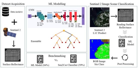
• Focusing on the problem of optical satellite image scene classification, an ensemble and Neural Network based ML models are proposed;
• An extended manually labeled Sentinel-2 database is set up by adding Surface Reflectance values to a previous available dataset;
• The diversity of the formulated dataset and the ML model sensitivity, biasness, and generalization ability are tested over geographically independent L1C images;
• The ML model benchmarking is performed against the existing Sen2Cor package that was developed for calibrating and classifying Sentinel-2 imagery.

2. Sen2Cor

While capturing satellite images, the atmosphere influences the spatial and spectral distribution of the electromagnetic radiation from the Sun before it reaches the Earth’s surface. As a result, the reflected energy recorded by a satellite sensor is affected and attenuated, requiring an atmospheric correction. Atmospheric correction is the process of removing the effects of the atmosphere on the Top-of-Atmosphere (TOA) reflectance values of original satellite images; TOA reflectance is a unitless measurement that provides the ratio between the radiation reflected and the incident solar radiation on a given surface. Bottom-Of-Atmosphere (BOA) reflectance, on the other hand, is defined as the fraction of incoming solar radiation that is reflected from Earth’s surface for a specific incident or viewing case.

Sen2Cor is an algorithm whose pivotal purpose is to correct single-date Sentinel-2 Level-1C products from the effects of the atmosphere and deliver a Level-2A surface reflectance product. Level-2A (L2A) output consists of a Scene Classification (SCL) image with eleven classes together with Quality Indicators for cloud and snow probabilities, Aerosol Optical Thickness (AOT) and Water Vapour (WV) maps and the surface (or BOA) reflectance images at different spatial resolutions (60 m, 20 m, and 10 m).

Table 1. List of Sen2Cor Scene Classification Classes and Corresponding Colors [34].

No.	Class	Color
0	No Data (Missing data on projected tiles) (black)
1	Saturated or defective pixel (red)
2	Dark features / Shadows (very dark gray)
3	Cloud shadows (dark brown)
4	Vegetation (green)
5	Bare soils / deserts (dark yellow)
6	Water (dark and bright) (blue)
7	Cloud low probability (dark gray)
8	Cloud medium probability (gray)
9	Cloud high probability (white)
10	Thin cirrus (very bright blue)
11	Snow or ice (very bright pink)

presents the eleven classes with their corresponding color representation in the SCL image. Each particular classification process [34] is discussed next.

2.1. Cloud and Snow

Figure 1 describes the Sen2Cor Cloud/Snow detection algorithm: it performs six tests and the result of each pixel is a cloud probability (ranging from 0 for high confidence clear sky to 1 for high confidence cloudy sky). After each step, the cloud probability of a potentially cloudy pixel is updated by multiplying the current pixel cloud probability by the result of the test. The snow detection follows the same procedure with five different tests resulting in 0 for high confidence clear (no snow) to 1 for high confidence snowy pixel.

2.2. Vegetation

Two filters, namely the Normalized Difference Vegetation Index ($NDVI$) [35] and a reflectance ratio (R), are used to identify vegetation pixels. The $NDVI$ and R filters are expressed by Equations (1) and (2) ($NIR$ (Near Infra-Red), $RED$ and $GREEN$ refer to the corresponding band values). Thresholds of $T1=0.40$ and $T2=2.50$ are set for $NDVI$ and R, respectively. If the $NDVI$ and R values exceed the corresponding thresholds, the pixel is classified as vegetation in the classification map.

$$NDVI=\frac{NIR-RED}{NIR+RED}$$

(1)

$$R=\frac{NIR}{GREEN}$$

(2)

2.3. Soil and Water

Bare soil pixels are detected when their reflectance ratio R (Equation (2)) falls below a threshold $T=0.55$. If the ratio $R1$ (Equation (3)) exceeds a threshold $T=4.0$ the pixel is classified as bright water.

$$R1=\frac{BLUE}{SWIR}$$

(3)

2.4. Cirrus Cloud

Under daytime viewing conditions, the presence of thin cirrus cloud in the upper troposphere is detected by Sentinel-2 band 10 (B10) reflectance threshold. In the first step, all B10 pixels with a value between $T=0.012$ and $T=0.035$ are considered as thin cirrus; in the second step, after generating a probabilistic cloud mask, if the cloud probability is below or equal to $0.35$, the pixel is classified as a thin cirrus cloud.

2.5. Cloud Shadow

The cloud shadow mask is constructed using (a) a “geometrically probable” cloud shadow derived from the final cloud mask, sun position and cloud height distribution and (b) a “radiometrically probable” cloud shadow derived from a neural network [36].

3. Materials and Methods

This study evaluates the performance of the developed machine learning models in classifying water, shadow, cirrus, cloud, snow, and other scenes over Sentinel-2 imagery. This section focuses on (a) Dataset creation; (b) Classification Algorithms; (c) Feature analysis and, finally, (d) Experimental setup and architecture modeling.

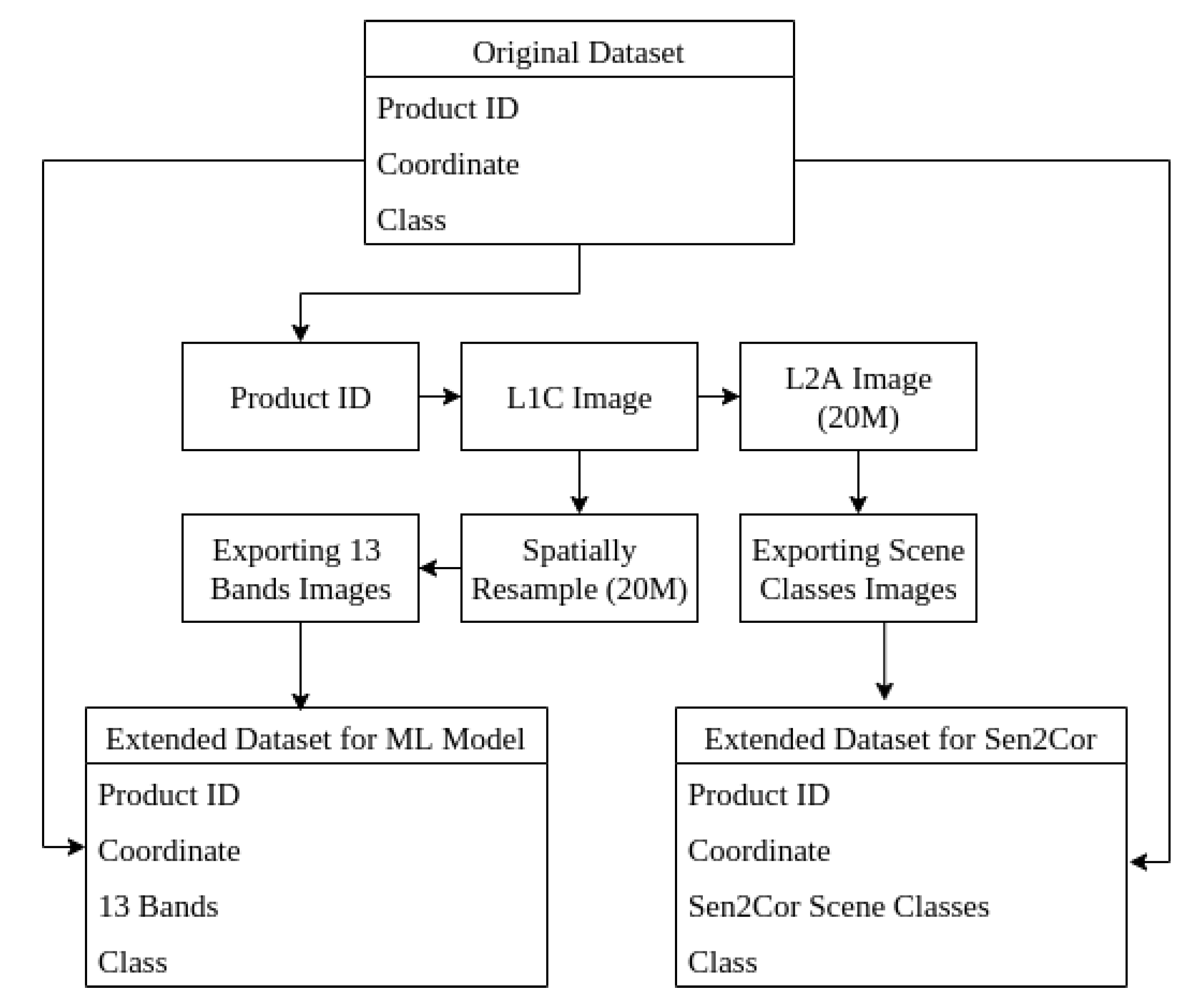
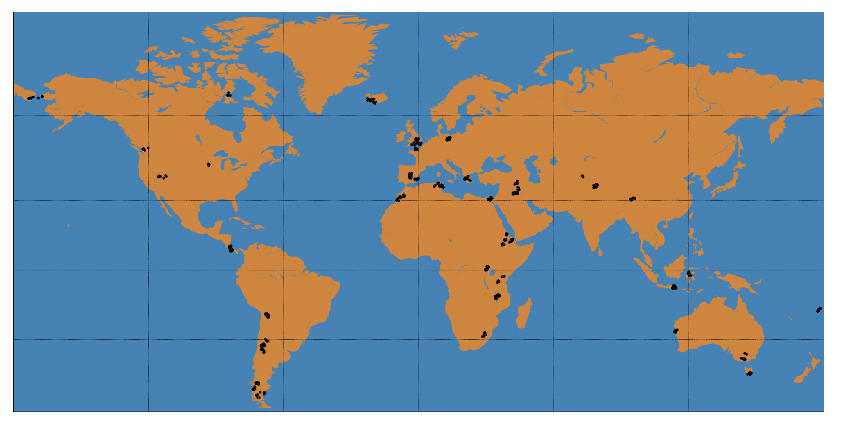
3.1. Dataset Creation

In supervised machine learning, input-label pairs are required by the learning function [37,38]. In this regard, the overall (input-label) dataset creation process is described in Figure 2, which perform the following steps:

• For each product-ID in the original dataset, L1C products were downloaded from CREODIAS [39] platform;
• For each downloaded L1C product, a corresponding L2A product was generated using Sen2Cor v2.5.5. Afterwards, for each L2A product, Scene Classification was retrieved resulting in an extended dataset for Sen2Cor assessment;
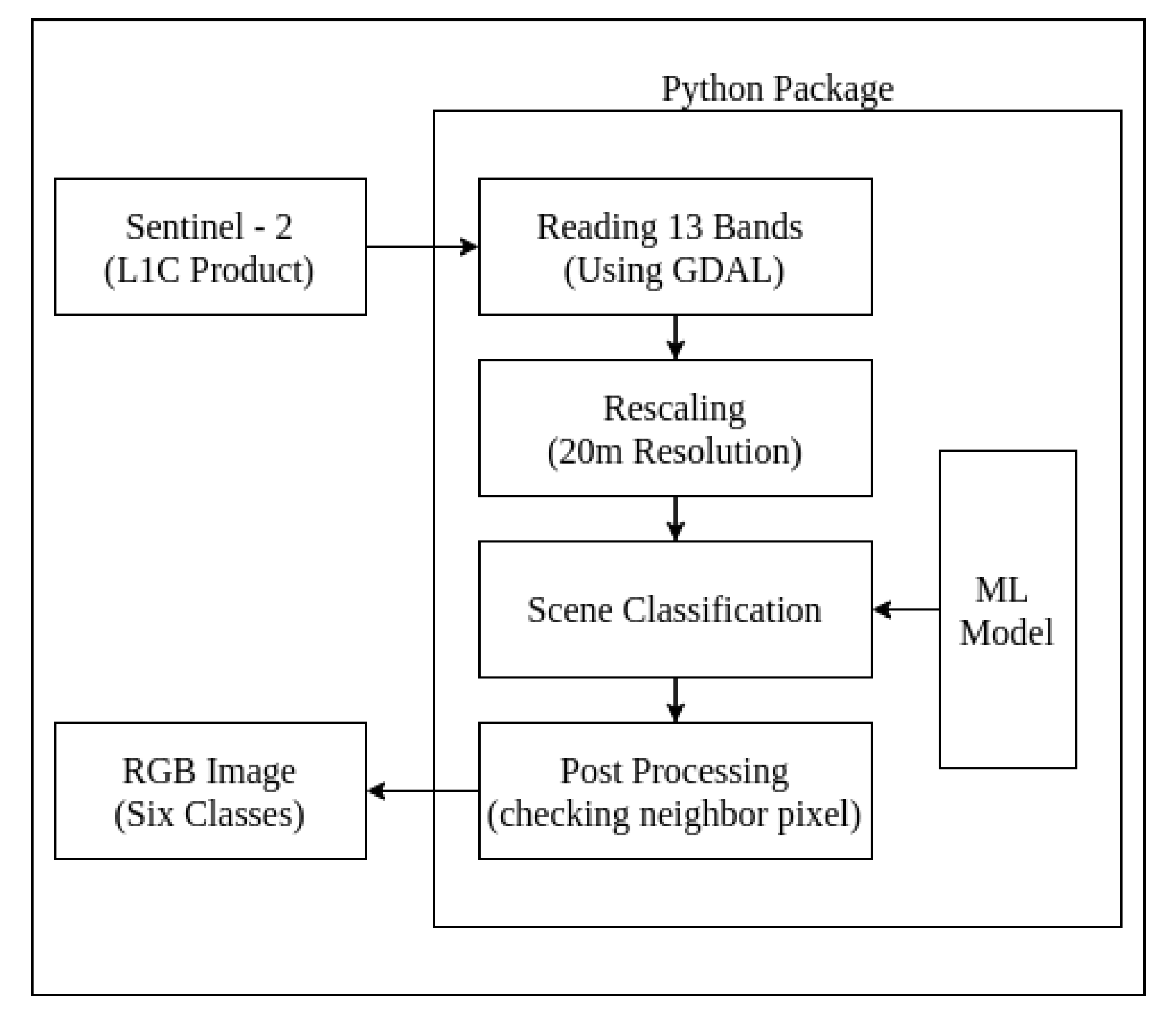
• Downloaded L1C products were re-sampled to 20 m (allowing spatial analysis) and the 13 bands of imagery were retrieved, resulting in an extended dataset for the ML model.

3.1.1. Original Data

Holstein et al. [40] created a database of manually labeled Sentinel-2 spectra using false-color RGB images. The database consists of images acquired over the entire globe (Figure 3) and comprises 6.6 million points (exactly 6,628,478 points) classified into one of the six classes presented in

Table 2. Holstein et al. [40] Dataset: Description of Classes with Coverage and Distribution of Points.

Class	Coverage	Points	Distribution (%)
Cloud	opaque clouds	1,031,819	15.57
Cirrus	cirrus and vapor trails	956,623	14.43
Snow	snow and ice	882,763	13.32
Shadow	clouds, cirrus, mountains, buildings	991,393	14.96
Water	lakes, rivers, seas	1,071,426	16.16
Other	remaining: crops, mountains, urban	1,694,454	25.56
Total	-	6,628,478	100

. It includes a wide range of surface types and geometry from a total of 60 products from the five different continents Europe (22), Africa (14), America (12), Asia (6) and Oceania (6). The data is described by 4 attributes: product_id, latitude, longitude and class.

As mentioned, Holstein et al. [40] used false-color RGB images to classify images. First of all, L1C products (all bands) were spatially resampled to 20 m. Afterwards, RGB bands 1, 3 and 8 were used to classify clouds and shadow, RGB bands 2, 8 and 10 were used to classify cirrus and water, and RGB bands 1, 7 and 10 were used to classify snow and other. Additionally, the authors used a two-step approach to minimize human error: the labeled images were revisited to re-evaluate past decisions.

3.1.2. Extended Data

Knowing L1C product ID and coordinates for individual data points, we added surface reflectance information to each entry to build and assess a Machine Learning classification model and further compare it to the Sen2Cor algorithm.

First of all, using the list of the 60 products from the original data, the relevant L1C products were downloaded using the CREODIAS [39] platform. Then, the L1C products were resampled to 20 m (allowing spatial analysis) and the 13 bands were retrieved for each product.

Extended Dataset for the ML model.

The extended data used to build the ML model is composed of 17 attributes: product_id, latitude, longitude, B01, B02, B03, B04, B05, B06, B07, B08, B8A, B09, B10, B11, B12, class. Here, B refers the band; each band represents the surface reflectance ($\rho$) value at a different wavelengths [41]. Surface reflectance is defined as the fraction of incoming solar radiation that is reflected from Earth’s surface for a specific incident or viewing case. In general, the reflectance values (also known as TOA) range from $0.0$ to $1.0$.

Figure 4 details the class-wise $\rho$ value distribution using the violin plot. Here, we can observe that for each class, the $\rho$ value for each band is different, meaning that each band has its $\rho$ value according to a different type of surface/class. For example, for all classes, B10 $\rho$ value is zero, apart from the Cirrus class; this is because B10 is responsible for the detection of thin cirrus [34].

In Figure 4, we can see that there are points from classes with $\rho$ greater than 1.0; unlike negative $\rho$, objects that have $\rho >1$ are not unnatural. Circumstances that would lead to such observance are: (a) nearby thunderstorm clouds that provide additional illumination from reflected solar radiation; (b) the area receiving solar radiation is directly perpendicular to the sun; and (c) surfaces such as shiny buildings, waves, or ice crystals that act as mirrors or lenses and reflect incoming direct sunlight in a concentrated way rather than diffusely.

Table 3. Extended Dataset: Point Distribution Overview of Band/Class wise Surface Reflectance ($\rho$) Greater than 1.0.

Bands\Class	Other	Water	Shadow	Cirrus	Cloud	Snow
B01	47	229	1076	5013	34,334	259,562
B02	587	313	2694	5589	47,265	285,053
B03	190	289	1232	3742	40,254	256,421
B04	536	429	3855	6897	79,380	300,538
B05	516	447	4300	8099	84,426	305,134
B06	546	477	4609	8597	993,355	299,270
B07	576	559	4653	8858	121,825	290,569
B08	517	424	3942	7880	96,182	277,403
B8A	607	597	4513	8903	133,901	281,007
B09	0	0	0	6	3730	60,674
B100	0	0	0	0	0	0
B11	597	0	1	0	10,112	0
B12	43	0	0	0	671	0
Total	4762 (0.02%)	3764 (0.03%)	30,875 (0.24%)	63,581 (0.51%)	751,415 (5.60%)	2,615,631 (22.79%)

presents the number of points of the dataset per band and class with $\rho >1$. We can observe that the class with a higher proportion of $\rho >1$ values is the Snow one. This can be explained taking into account that snowy surfaces reflect incoming sunlight in a concentrated way rather than diffusely acting as a mirror, producing observed $\rho >1$.

Extended Dataset for Sen2Cor assessment.

The data used for assessing Sen2cor algorithm is composed of 5 attributes: product_id, latitude, longitude, sen2cor_class, class. Since there are eleven classes in Sen2cor scene image (Table 1) and only six classes in original data (Table 2), a class mapping was performed. This mapping is shown in

Table 4. Class Mapping of Extended Dataset for Sen2Cor Assessment.

Mapped Class	Corresponding Sen2Cor Class (Table 1)
Cloud	Cloud high probability
Cirrus	Thin Cirrus
Snow	Snow
Shadow	Shadow, Cloud Shadow
Water	Water
Other	No Data, Defective Pixel, Vegetation, Soil, Cloud low and medium probability

.

3.2. Classification Algorithms

In this study, we evaluated ensemble methods (Random Forest & Extra Tree) and a deep learning based method (Convolutional Neural Network) using the built extended dataset for satellite imagery scene classification. This section introduces shortly the used classification algorithms and provides details about feature analysis and the adopted experimental setup.

During the ML modeling process, the following statistical and CNN-based classifications algorithms were used.

3.2.1. Decision Tree (DT)

Decision tree is an efficient inductive machine learning technique [42,43] where the model is trained by recursively splitting the data [44]. The data splitting consists of a tree structure (root-nodes-branches-leaf), which successively tests features of the dataset at each node and splits the branches with different outcomes. This process continues until a leaf (or terminal node) representing a class is found. Each split is chosen according to an information criterion which is maximized (or minimized) by one of the “splitters”.

However, a decision tree is sensitive to where it splits and how it splits. Generally, the bias-variance trade-off depends on the depth of the tree: a complex decision tree (e.g., deep) has a low bias and a high variance. Also, the tree makes almost no assumptions about the target function but it is highly susceptible to variance in data making decision trees prone to overfit [45].

Decision trees were used in many applications, including identification of land cover change [46], mapping of global forest change [47] and differentiating five palustrine wetland types [48].

3.2.2. Random Forest (RF)

Random Forest (RF) is a tree ensemble algorithm [49], which aims to reduce the decision tree variance (at the small cost of bias). During the random forest learning process, bagging is used to minimize the variance by learning from several trees over various sub-samples of the data [50] (in terms of both observations and predictors used to train them). Bagging is a process where several decisions are averaged [51].

In the random forest learning process [45], m variables are randomly selected from a potential set of p variables, resulting in two groups that separate the data in the best way possible. This process is repeated to the max depth of d, creating a forest of several individual trees. In the end, observation x is classified using all the individual trees, and the final decision is averaged.

3.2.3. Extra Tree (ET)

The main difference between a random forest and extra tree [52] (usually called extreme random forests) lies in the fact that, instead of computing the locally optimal feature/split combination (for the random forest), for each feature under consideration, a random value is selected for the split [53]. This leads to more diversified trees and fewer splitters to evaluate when training.

3.2.4. Convolutional Neural Networks (CNNs)

CNNs are Neural Networks that receive an input, assign importance (learnable weights and biases) to various aspects/objects within the input, and are able to differentiate one input from other. Due to the sparse interactions and weight sharing, Neural Networks (NN) are best suited for processing large-scale imagery [54]. When considering CNNs, the connection between the previous layer and the next layer is referred to as sparse interaction. Whereas, in weight sharing, layer share the same connection weights.

Recently researchers are proposing complex and deeper structures like, for example, AlexNet [55], VGGNet [56], and GoogLeNet [57], having depths of 8, 19, and 22, respectively [58]. In other words, CNN exploits domain knowledge about feature invariances within its structure and they have been successfully applied to various image analysis and recognition tasks [59], making it an effective technique for labeled tabular data classification [60].

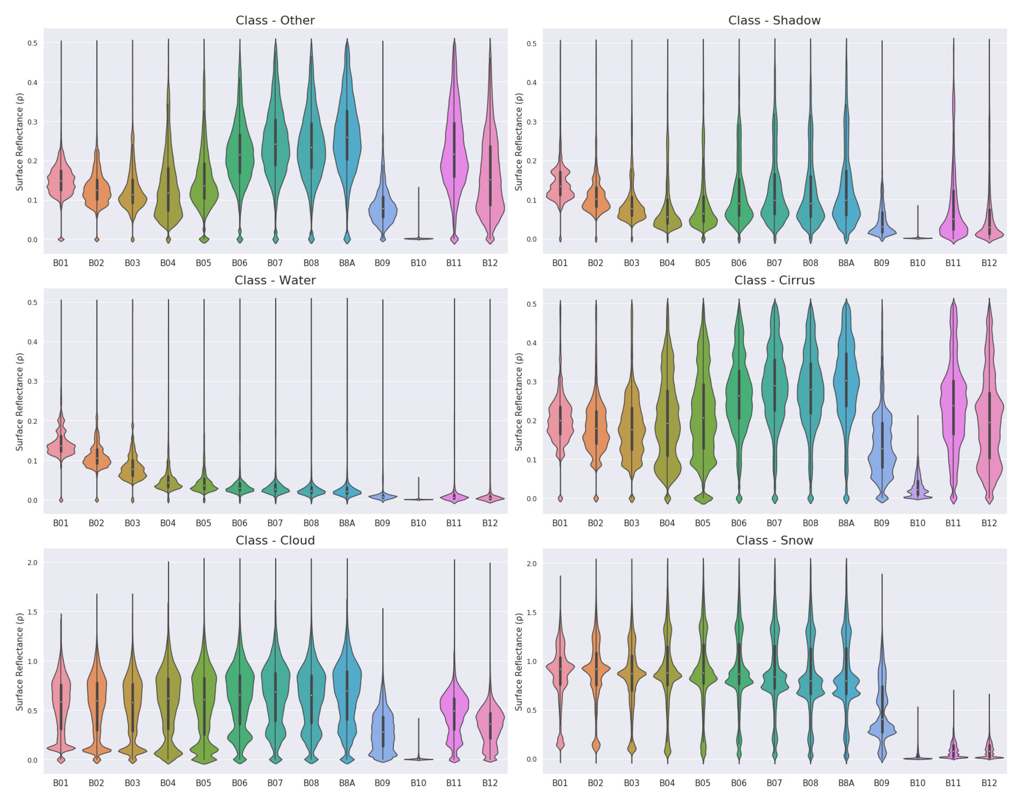
3.3. Feature Analysis

Feature ranking helps to select the most useful features to build a model. The Scikit-Learn library [61] provides an implementation of the most useful statistical algorithms for feature ranking [62], including Chi-Squared (chi2) [63], Mutual Information (mutual info.) [64], ANOVA (anova) [65] and Pearson’s Correlation Coefficient (pearson) [66]. We applied these measures over the full dataset and the ranking is shown in

Table 5. Feature Analysis: Feature Ranking using Statistical Algorithms.

Rank	Chi2	Mutual Info.	Anova	Pearson
1	B11	B11	B11	B11
2	B12	B01	B12	B12
3	B04	B12	B8A	B8A
4	B8A	B02	B07	B07
5	B03	B03	B08	B08
6	B07	B04	B03	B03
7	B05	B06	B06	B06
8	B02	B05	B01	B01
9	B08	B07	B02	B02
10	B06	B8A	B04	B04
11	B01	B08	B05	B05
12	B09	B09	B09	B09
13	B10	B10	B10	B10

.

Sen2Cor uses nine bands (1, 2, 3, 4, 5, 8, 10, 11 and 12) to generate a scene classification map and ten bands (1, 2, 3, 4, 8, 8A, 9, 10, 11 and 12) to produce a L2A product [34]. Comparing this band information with the results shown in Table 5 and the surface reflectance ($\rho$) values distribution (Figure 4), the obtained statistical feature ranking produces contradictory results. For example, statistical feature ranking ranks B10 as the least important band, but the sole purpose of B10 is to identify the presence of the Cirrus class, which is supported by Figure 4. Removing B10 from the training dataset can hinder the model performance when applied on an unseen (satellite) image acquired from anywhere over the globe. This fact leads us to state that although the dataset is a collection over different continents and represent a possible global distribution, ranking bands upon the dataset is not ideal as each band has its own purpose/reflectance. Thus, in our experiments, we have used all the 13 bands to possibly cover all the surface reflectance ($\rho$) value distributions.

3.4. Experimental Setup

To assess the classifiers, 10 products (belonging to all five continents: one each from Asia and Oceania, two each from Africa and America, and four from Europe) out of 60 were randomly selected for the test set. Aiming at including all 5 continents in the test set led to a class distribution somehow different from the full dataset. The test set distribution can be seen in

Table 6. Test set: Class-wise Point Distribution (%).

Class	Points	Distribution (%)
Other	174,369	10.29
Water	117,010	10.92
Shadow	155,715	15.71
Cirrus	175,988	18.40
Cloud	134,315	13.02
Snow	154,751	17.53
Total	912,148	13.76

.

The information about the experimental setup used to build the classifiers is presented in

Table 7. Experimental Settings and System Specifications.

Attribute	Description
Features	13 (value of each band)
Classes	6 (Other, Water, Shadow, Cirrus, Cloud, Snow)
Training set	50 Products (5,716,330 samples)
Test set	10 Products (912,148 samples)
Language and Library	Python and Scikit-learn
System Specification	Intel(R) Xeon(R) Silver 4110 CPU @ 2.10GHz
CNN Early Stopping	monitor = ’val_loss’, mode = ’min’, patience = 2
CNN Model Checkpoint	monitor = ’val_acc’, mode = ’max’

.

Precision, recall and F1 score are performance measures that can be used to evaluate ML models. Precision is defined as the ratio between the number of correct positive and all positive results whereas, in recall all relevant samples (all samples that should have been identified as positive) are considered instead of all positive results [67]; F1 is the harmonic mean of Precision and Recall. These measures are calculated per class (considering one class as positive and all the other classes as negative) using Equations (4).

$$\begin{array}{c}\hfill Precision=\frac{TP}{TP+FP}Recall=\frac{TP}{TP+FN}F1=2🟉\frac{Precision🟉Recall}{Precision+Recall}\end{array}$$

(4)

Here, $TP$, $TN$, $FP$, and $FN$ stand for True Positive, True Negative, False Positive, and False Negative.

When aiming to have an unique performance value, precision, recall and F1 are averaged; this average can be calculated over the per class values (macro-average) or by summing the true positive, false positive and false negative for all classes and calculating the performance measures over these counts (micro-average).

To fine-tune the classification algorithms, a RandomizedSearchCV [68] with 5 folds cross-validation procedure over the train set was used. The assessment was done using the micro-F1 measure.

Table 8. Fine-tune Parameter values for Random Forests (RF) and Extra Trees (ET) Algorithms.

Parameter	RF	ET
criterion	gini	gini
max_depth	20	20
min_samples_split	50	10
min_samples_leaf	1	1
max_features	sqrt	sqrt
n_estimators	242	279
min_samples_split	50	10
bootstrap	True	True

shows the best parameter values for Random Forests (RF) and Extra Trees (ET) algorithms. The found CNN parameter values were $epochs=8$, $batchsize=32$, $filters=24$ and, $kernelsize=4$.

Figure 5 shows the CNN model structure. Using the CNN architecture [69] as a base reference, the used CNN model consists of an input layer, 1D convolutional layers, a dropout layer, a max-pooling layer, followed by one flatten, two dense, and an output layer.

Following is a description of each layer:

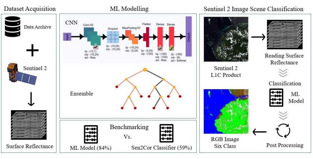
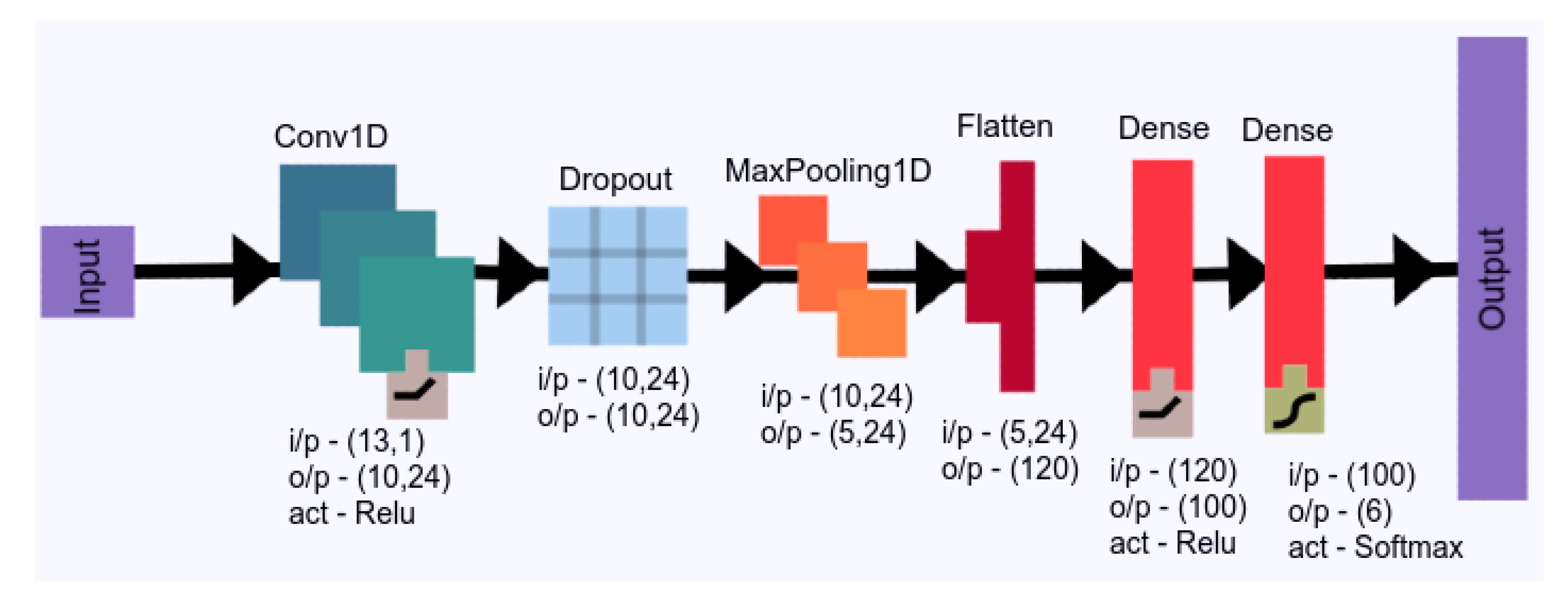
• Input layer: The input representation of this layer is a matrix value of 13 bands;
• Convolutional-1D layer: This layer is used to extract features from input. Here, from the previous layer, multiple activation feature maps are extracted by combining the convolution kernel. In our architecture, we used a convolution kernel size of 4;
• Dropout: A random portion of the outputs for each batch is nullified to avoid strong dependencies between portions of adjacent layers;
• Pooling layer: This layer is responsible for the reduction of dimension and abstraction of the features by combining the feature maps. Thus, the overfitting problem is prevented, and at the same time, computation speed is increased;
• Flatten layer: Here, the (5 × 24) input from the previous layer is taken and transformed into a single vector giving a feature space of width 120;
• Dense layer: In this layer, each neuron receives input from all the neurons in the previous layer, making it a densely connected neural network layer. The layer has a weight matrix W, a bias vector b, and the activation function of the previous layer.
• Softmax activation: It is a normalized exponential function which is used in multinomial logistic regression. By using the softmax activation function, the last output vector of the CNN model is forced to be a part of the sample class (in our case, the output vector is 6).

4. Results

As mentioned in the previous section, the classification models were compared over the test set that comprises 10 products from all five continents.

Table 9. Results over the test set: Random Forest (RF), Extra Trees (ET), Convolutional Neural Network (CNN) and Sen2Cor (SCL). The proposed models ET and CNN achieves a micro-F1 value of $0.84$ compared to the Sen2Cor of $0.59$.

Class	Precision				Recall				Micro-F1				Support
	RF	ET	CNN	SCL	RF	ET	CNN	SCL	RF	ET	CNN	SCL
Other	0.74	0.74	0.74	0.39	0.91	0.96	0.92	0.97	0.82	0.83	0.82	0.56	174,369
Water	0.96	0.93	0.93	0.84	0.86	0.87	0.87	0.83	0.91	0.90	0.90	0.84	117,010
Shadow	0.89	0.91	0.91	0.96	0.77	0.73	0.75	0.54	0.83	0.81	0.83	0.69	155,715
Cirrus	0.78	0.82	0.78	0.91	0.67	0.76	0.75	0.10	0.72	0.79	0.76	0.18	175,988
Cloud	0.77	0.81	0.79	0.62	0.91	0.90	0.90	0.94	0.83	0.86	0.84	0.75	134,315
Snow	0.93	0.94	0.96	0.86	0.88	0.86	0.86	0.31	0.90	0.90	0.91	0.46	154,751
Overall	0.83	0.84	0.84	0.59	0.83	0.84	0.84	0.59	0.83	0.84	0.84	0.59	912,148

shows precision, recall and micro-F1 values for Random Forests (RF), Extra Trees (ET), Convolutional Neural Networks (CNN) along with Sen2Cor Scene Classification (SCL).

Analysing Table 9, the following observations can be made:

• When looking at micro-F1, CNN performs similar to Random Forest and Extra Trees. The difference in micro-F1 is small (almost zero) and we cannot state that CNN outperforms the others. Moreover, one can state that each algorithm performs better than the others on specific classes; for example, ET has higher micro-F1 over classes Cirrus, Cloud, and Other, whereas RF has higher micro-F1 over Water and CNN over Snow.
• Looking at precision and recall for Cirrus and Shadow classes, it is noticeable that Sen2Cor has high precision but low recall. This means that Sen2Cor is returning very few results of Cirrus and Shadow (it has a very high rate of false negatives), although most of its predicted labels are correct (low level of false positive errors).
• Overall, the three Machine Learning algorithms generate models with similar performance with differences that range from 0% to 7% between the “best” and the “worst”. (for example, Cirrus has a “best” micro-F1 of 0.79% with ET and a “worst” micro-F1 of 0.72% with RF.) With regard to the classes, there is a great variation: precision values are above 90% for classes Snow and Shadow and less than 75% for the Other class; for recall, the highest values are obtained for the classes Cloud and Other (values above 80%) and the lowest for the Cirrus and Shadow classes (values between 67% and 77%). Regarding the micro-F1 measure, the only class with values below 80% is the class Cirrus; classes Snow and Water have values above 90%.
• Comparing the performance of ML algorithms with Sen2Cor, especially for the Cirrus and Snow classes, ML approaches are superior. For the same classes, Sen2Cor micro-F1 values are below 50%; these low values are due to the big difference between precision and recall (for Cirrus precision is above 90% while recall is 10%; for Snow precision is above 85% and recall around 30%). Considering the micro-F1 measure, the ML models present an increase of about 25 points (from 59% to 84%) when compared to the Sen2Cor Scene Classification algorithm.

To check if there is a significant difference between Sen2Cor and ML models (i.e., if the difference in micro-F1 is significant or not), the McNemar-Bowker test [70,71] was performed. The McNemar-Bowker’s test is a statistical test used on paired nominal data (with $k\times k$ contingency tables following a dichotomous trait) to determine if there is a difference between two related groups. Here, k is the number of categories/labels, and the McNemar-Bowker B value is calculated using the Equation (5), where, $O_{i,j}$ is the count of the $i^{th}$ row and $j^{th}$ column in crosstab. A crosstab is a table that shows the relationship between $k\times k$ variables.

$$B=\sum _{i=1}^{k-1}\sum _{j=i+1}^k\frac{{(O_{i,j}-O_{j,i})}^2}{(O_{i,j}+O_{j,i})}$$

(5)

The acquired B value follows approximately a chi-square distribution [72], with $df=(k-1)/2$ degrees of freedom. The probability density function is be calculated using Equation (6), where, $\Gamma$ denotes the gamma function, which has closed-form values for integer $(df/2)$.

$$f(B,df)=\frac{B^{df/2-1}{e}^{-B/2}}{2^{df/2}\Gamma (df/2)}$$

(6)

Using Equation (6) for comparing Sen2Cor and ML models, our null hypothesis (the difference between two groups is statistically significant) was proved by obtaining a $(p$-value) less-then 0.05. The same can be visualized in Figure 6 where a value of McNemar-Bowker B = 271,184 and degrees of freedom $df=15$ result in $(p$-value) = 0.0.

To have a better grasp of the differences between the ML model and Sen2Cor, we randomly selected an image (Figure 7a) from the test set with classes Cloud, Shadow, and Other (identified as white, brown, and green respectively) and generated classification images using the ET model (Figure 7b) and Sen2cor (Figure 7c). The original image and the resulting classified images are presented in Figure 7.

After analysing Figure 7a closely, it is possible to say that for each cloud present in the image there is an equivalent shadow. Comparing the generated images of Figure 7b, we can observe that the ML model is classifying cloud and cloud shadow accurately than Sen2Cor; Sen2Cor classification (Figure 7c) is missing the majority of cloud shadows, whereas the ML model captures them all.

We state that a static rule-based approach, like the one used by Sen2Cor that heavily rely on surface reflectance (it uses a sensor-specific threshold based method) tends to miss marginal variation between two surfaces leading to misclassification. To support this claim and to prove the general-ability of the ML model, we classified a specific image (Figure 8) with brighter surface reflectance values (note that this image does not belong to the dataset). Figure 8a shows the RGB image of the coastal area of Lisbon, Portugal; in it, there are 3 visible parts: water, coastal area sand and land surface. Figure 8b,c show the generated classification images using the ET model and Sen2Cor, respectively.

After analysing Figure 8 closely, it is possible to say that the bright coastal area/sand present in the Figure 8a is classified as Cloud by Sen2Cor (represented as a white line); on the other hand, the ML algorithm classified the same bright coastal area/sand as Other which is indeed is the correct classification. Thus, the ML model is able to better capture brighter coastal surface reflectance values when compared to Sen2Cor.

5. Discussion

Our proposed system uses a dynamic and generalized approach of surface reflectance, which does not rely on predefined threshold rules. Thus, we are preserving the pivotal motivation of classifying any unseen Sentinel-2 images acquired from the globe.

Further, ensemble methods can provide useful information like the Gini index to the end-user. The Gini index is a measure of statistical distribution intended to represent different attribute variables influencing the overall accuracy [73]. Using the Gini index, we were able to identify that B11 and B12 have a substantial effect on the overall model accuracy (data not presented). Thus, using our proposed model, the classification performance can be increased by including additional indexes [74], that use Band 11 and Band 12. For example, including Global Vegetation Index (GVI) [75], Normalized Difference Salinity Index (NDSI) [76], and Soil Composition Index (SCI) [77] would help in getting a better performance.

Overall, the random forest and extra tree algorithms produce fast and accurate predictions (with micro-F1 between 0.83 and 0.84). Nonetheless, when using these ensemble methods, the issues of overfitting, and bias/variance tradeoff should not be overlooked.

Since Figure 7b shows shadows of all the clouds, we analyzed the the sensitivity of the ML model. For that we randomly selected (not from dataset) three separate L1C image patches shown in Figure 9a (Ballyhaunis, Ireland), Figure 9b (Sukabumi. Indonesia), and Figure 9c (Béja, Tunisia). Then we applied the ET classifier to check if the classifier was too “pedantic”.

From Figure 9 it can be observed that for each geometric independent region (Ballyhaunis, Sukabumi, and Béja), the ML model is capturing, with high precision, the shadows of the (low, medium, and opaque) clouds, proving the general-ability of the ML model. To this extent, we can say that the ML models are sensitive and can detect even minor shadows (from low and medium probability clouds). Moreover, the detection of shadow does not decrease the workable area as the classifier is generating a mask and the end-user can still use these workable areas given they might belong to the ’shadow’ or ’cloud’ class.

Further, we studied the biasness of the model towards the achieved results. To do so, we selected 59 products for training and 1 for testing. The main reason to split the dataset in this way was to make sure that the knowledge about a region is not essential to classify that region. This reasoning enables to pose the following question: ’will the system be able to classify a new, non seen product with high performance?’ To evaluate this, it would be interesting to pick a complete region as test while the rest of the points compose the training set.

We replicated this procedure for each of the 60 products (i.e., using 1 product for test and the rest 59 products for training). The $F{1}_{avg}$ results are presented in

Table 10. Scene Biasness Test Results: $F{1}_{avg}$ values of ML algorithms and Sen2Cor.

Class	DT	RF	ET	CNN	Sen2Cor	Support
Other	63.29	72.3	74.16	74.43	64.96	1,694,454 (25.56%)
Water	63.81	73.4	76.69	73.88	80.73	1,071,426 (16.16%)
Shadow	53.98	63.96	61.45	64.63	50.57	991,393 (14.96%)
Cirrus	47.58	56.63	42.97	51.58	24.08	956,623 (14.43%)
Cloud	65.25	75.08	75.33	72.67	75.04	1,031,819 (15.57%)
Snow	74.67	84.90	87.00	83.43	61.40	882,763 (13.32%)
$F{1}_{avg}$	67.95	76.43	76.77	77.54	66.40	6,628,478 (100%)

.

Equation (7) calculates the $F{1}_{avg}$ value (over 60 products) for each class where $F{1}_p$ is the $F1$ value of the particular class within the product p. $N_p$ is the number of points of the class within the product p, T is the total number of points of the class for all products, and $p\in (1,60)$ is the number of products.

$$\begin{array}{c}\hfill F{1}_{avg}=\sum _{p=1}^{60}\left(F{1}_p\times N_p\right)÷TwithT=\sum _{p=1}^{60}{N}_p\end{array}$$

(7)

When compared to the Sen2Cor, the ML approach achieved an overall improvement of 11% (77.54% with CNN, 66.40% with Sen2Cor). This study ensures that the achieved results are better due to the learning done by the algorithms, and that the proposed models do not possess biasness towards the test set.

Regarding the neural network architecture, different CNN-based models were proposed to classify cloud mask and land cover change using different spectral and temporal resolutions satellite imagery [1,21,22]. These studies look at different datasets and present different CNN architectures but, to the best of our knowledge, none evaluates the CNN architecture with the dataset used in this work making it impossible to make a comparison of the obtained results.

6. Conclusions

The significant development of remote sensing technology over the past decade has enabled us for intelligent Earth observation, such as scene classification using satellite images. However, the lack of publicly available “large and diverse data sets” of remote sensing images severely limits the development of new approaches especially Machine Learning methods. This paper first presents a comprehensive review of the recent progress in the field of remote sensing image scene classification, including existing data sets and Sen2Cor. Then, by analyzing the limitations of the existing data sets, it introduces a surface reflectance based, freely and publicly available data set and makes available a ready to use Python package(scripts) (refer Appendix A) with a trained ML model. These will enable the scientific community to develop and evaluate new data-driven algorithms to classify Sentinel-2 L1C images into six classes (Water, Shadow, Cirrus, Cloud, Snow, and Other).

Using the micro-F1 measure, we evaluated three ML representative algorithms (Random Forest, Extra Tree and Convolution Neural Network) for the task of scene classification using the proposed data set and reported the results as a useful (baseline) performance for future research. The proposed ML model presents a micro-F1 value of $0.84$, a considerable improvement over Sen2Cor that reached a value of $0.59$.

The results presented in Table 9 support our claim that the developed ML model can be used as a base tool for Sentinel-2 optical image scene classification. Moreover, when evaluating over one complete test set image (Figure 7), it is possible to conclude that while Sen2Cor misses the majority of cloud shadows, the ML model captures them. Additionally, model sensitivity (Figure 9) and biasness (Table 10) tests were performed over different L1C images.

Being composed of several modules, each of them with a high level of complexity, it is certain that our approach can still be improved and an overall higher performance is achievable. As future work, we intend not only to continue improving the individual modules, but also extend this work to:

• Add more training scenes with the help of image augmentation (also known as elastic transformation) [78] using existing training data.
• Incorporate radar information and correlate the results and its impact over Water, Shadow, Cirrus, Cloud, and Snow detection.
• Study different CNN architectures.

References

1. Mohajerani, S.; Krammer, T.A.; Saeedi, P. Cloud detection algorithm for remote sensing images using fully convolutional neural networks. arXiv 2018, arXiv:1810.05782. [Google Scholar]
2. Hashem, N.; Balakrishnan, P. Change analysis of land use/land cover and modelling urban growth in Greater Doha, Qatar. Ann. GIS 2015, 21, 233–247. [Google Scholar] [CrossRef]
3. Rahman, A.; Kumar, S.; Fazal, S.; Siddiqui, M.A. Assessment of land use/land cover change in the North-West District of Delhi using remote sensing and GIS techniques. J. Indian Soc. Remote Sens. 2012, 40, 689–697. [Google Scholar] [CrossRef]
4. Liou, Y.A.; Nguyen, A.K.; Li, M.H. Assessing spatiotemporal eco-environmental vulnerability by Landsat data. Ecol. Indic. 2017, 80, 52–65. [Google Scholar] [CrossRef] [Green Version]
5. Nguyen, K.A.; Liou, Y.A. Mapping global eco-environment vulnerability due to human and nature disturbances. MethodsX 2019, 6, 862–875. [Google Scholar] [CrossRef] [PubMed]
6. Dao, P.D.; Liou, Y.A. Object-based flood mapping and affected rice field estimation with Landsat 8 OLI and MODIS data. Remote Sens. 2015, 7, 5077–5097. [Google Scholar] [CrossRef] [Green Version]
7. San, B.T. An evaluation of SVM using polygon-based random sampling in landslide susceptibility mapping: The Candir catchment area (Western Antalya, Turkey). Int. J. Appl. Earth Obs. Geoinf. 2014, 26, 399–412. [Google Scholar] [CrossRef]
8. Sentinel-2 Mission. Available online: https://sentinel.esa.int/web/sentinel/missions/sentinel-2 (accessed on 4 February 2020).
9. European Copernicus Programme. Available online: https://www.copernicus.eu/en (accessed on 22 June 2020).
10. Frantz, D.; Haß, E.; Uhl, A.; Stoffels, J.; Hill, J. Improvement of the Fmask algorithm for Sentinel-2 images: Separating clouds from bright surfaces based on parallax effects. Remote Sens. Environ. 2018, 215, 471–481. [Google Scholar] [CrossRef]
11. Main-Knorn, M.; Louis, J.; Hagolle, O.; Müller-Wilm, U.; Alonso, K. The Sen2Cor and MAJA cloud masks and classification products. In Proceedings of the 2nd Sentinel-2 Validation Team Meeting, ESA-ESRIN, Frascati, Rome, Italy, 29–31 January 2018; pp. 29–31. [Google Scholar]
12. Zhu, Z.; Woodcock, C.E. Object-based cloud and cloud shadow detection in Landsat imagery. Remote Sens. Environ. 2012, 118, 83–94. [Google Scholar] [CrossRef]
13. Zhu, Z.; Woodcock, C.E. Automated cloud, cloud shadow, and snow detection in multitemporal Landsat data: An algorithm designed specifically for monitoring land cover change. Remote Sens. Environ. 2014, 152, 217–234. [Google Scholar] [CrossRef]
14. Hagolle, O.; Huc, M.; Pascual, D.V.; Dedieu, G. A multi-temporal method for cloud detection, applied to FORMOSAT-2, VENμS, LANDSAT and SENTINEL-2 images. Remote Sens. Environ. 2010, 114, 1747–1755. [Google Scholar] [CrossRef] [Green Version]
15. Petrucci, B.; Huc, M.; Feuvrier, T.; Ruffel, C.; Hagolle, O.; Lonjou, V.; Desjardins, C. MACCS: Multi-Mission Atmospheric Correction and Cloud Screening tool for high-frequency revisit data processing. In Image and Signal Processing for Remote Sensing XXI; International Society for Optics and Photonics: Bellingham, WA, USA, 2015; Volume 9643, p. 964307. [Google Scholar]
16. Moustakidis, S.; Mallinis, G.; Koutsias, N.; Theocharis, J.B.; Petridis, V. SVM-based fuzzy decision trees for classification of high spatial resolution remote sensing images. IEEE Trans. Geosci. Remote Sens. 2011, 50, 149–169. [Google Scholar] [CrossRef]
17. Munoz-Mari, J.; Tuia, D.; Camps-Valls, G. Semisupervised classification of remote sensing images with active queries. IEEE Trans. Geosci. Remote Sens. 2012, 50, 3751–3763. [Google Scholar] [CrossRef]
18. Oliva, A.; Torralba, A. Modeling the shape of the scene: A holistic representation of the spatial envelope. Int. J. Comput. Vis. 2001, 42, 145–175. [Google Scholar] [CrossRef]
19. Ojala, T.; Pietikainen, M.; Maenpaa, T. Multiresolution gray-scale and rotation invariant texture classification with local binary patterns. IEEE Trans. Pattern Anal. Mach. Intell. 2002, 24, 971–987. [Google Scholar] [CrossRef]
20. Hu, F.; Xia, G.S.; Hu, J.; Zhang, L. Transferring deep convolutional neural networks for the scene classification of high-resolution remote sensing imagery. Remote Sens. 2015, 7, 14680–14707. [Google Scholar] [CrossRef] [Green Version]
21. Li, Z.; Shen, H.; Cheng, Q.; Liu, Y.; You, S.; He, Z. Deep learning based cloud detection for medium and high resolution remote sensing images of different sensors. ISPRS J. Photogramm. Remote Sens. 2019, 150, 197–212. [Google Scholar] [CrossRef] [Green Version]
22. Zhang, C.; Sargent, I.; Pan, X.; Li, H.; Gardiner, A.; Hare, J.; Atkinson, P.M. Joint Deep Learning for land cover and land use classification. Remote Sens. Environ. 2019, 221, 173–187. [Google Scholar] [CrossRef] [Green Version]
23. Baetens, L.; Desjardins, C.; Hagolle, O. Validation of Copernicus Sentinel-2 Cloud Masks Obtained from MAJA, Sen2Cor, and FMask Processors Using Reference Cloud Masks Generated with a Supervised Active Learning Procedure. Remote Sens. 2019, 11, 433. [Google Scholar] [CrossRef] [Green Version]
24. Hagolle, O.; Huc, M.; Desjardins, C.; Auer, S.; Richter, R. Maja Algorithm Theoretical Basis Document. 2017. Available online: https://zenodo.org/record/1209633#.XpdnZvnQ-Cg (accessed on 4 August 2020).
25. Louis, J.; Debaecker, V.; Pflug, B.; Main-Knorn, M.; Bieniarz, J.; Mueller-Wilm, U.; Cadau, E.; Gascon, F. Sentinel-2 Sen2Cor: L2A processor for users. In Proceedings of the Living Planet Symposium 2016, Spacebooks Online, Prague, Czech Republic, 9–13 May 2016; pp. 1–8. [Google Scholar]
26. Qiu, S.; Zhu, Z.; He, B. Fmask 4.0: Improved cloud and cloud shadow detection in Landsats 4–8 and Sentinel-2 imagery. Remote Sens. Environ. 2019, 231, 111205. [Google Scholar] [CrossRef]
27. Zou, Q.; Ni, L.; Zhang, T.; Wang, Q. Deep learning based feature selection for remote sensing scene classification. IEEE Geosci. Remote Sens. Lett. 2015, 12, 2321–2325. [Google Scholar] [CrossRef]
28. Yang, Y.; Newsam, S. Bag-of-visual-words and spatial extensions for land-use classification. In Proceedings of the 18th SIGSPATIAL International Conference on Advances in Geographic Information Systems, San Jose, CA, USA, 2–5 November 2010; pp. 270–279. [Google Scholar]
29. Xia, G.S.; Hu, J.; Hu, F.; Shi, B.; Bai, X.; Zhong, Y.; Zhang, L.; Lu, X. AID: A benchmark data set for performance evaluation of aerial scene classification. IEEE Trans. Geosci. Remote Sens. 2017, 55, 3965–3981. [Google Scholar] [CrossRef] [Green Version]
30. Penatti, O.A.; Nogueira, K.; Dos Santos, J.A. Do deep features generalize from everyday objects to remote sensing and aerial scenes domains? In Proceedings of the IEEE Conference on Computer Vision and Pattern Recognition Workshops, Boston, MA, USA, 7–12 June 2015; pp. 44–51. [Google Scholar]
31. Helber, P.; Bischke, B.; Dengel, A.; Borth, D. Eurosat: A novel dataset and deep learning benchmark for land use and land cover classification. IEEE J. Sel. Top. Appl. Earth Obs. Remote Sens. 2019, 12, 2217–2226. [Google Scholar] [CrossRef] [Green Version]
32. Zhou, W.; Newsam, S.; Li, C.; Shao, Z. PatternNet: A benchmark dataset for performance evaluation of remote sensing image retrieval. ISPRS J. Photogramm. Remote Sens. 2018, 145, 197–209. [Google Scholar] [CrossRef] [Green Version]
33. Sumbul, G.; Charfuelan, M.; Demir, B.; Markl, V. Bigearthnet: A large-scale benchmark archive for remote sensing image understanding. In Proceedings of the IGARSS 2019—2019 IEEE International Geoscience and Remote Sensing Symposium, Yokohama, Japan, 28 July–2 August 2019; pp. 5901–5904. [Google Scholar]
34. Sentinel-2 MSI—Level 2A Products Algorithm Theoretical Basis Document. Available online: https://earth.esa.int/c/document_library/get_file?folderId=349490&name=DLFE-4518.pdf (accessed on 4 February 2020).
35. Rouse, J.; Haas, R.; Schell, J.; Deering, D. Monitoring vegetation systems in the Great Plains with ERTS. NASA Spec. Publ. 1974, 351, 309. [Google Scholar]
36. Kohonen, T. Self-organized formation of topologically correct feature maps. Biol. Cybern. 1982, 43, 59–69. [Google Scholar] [CrossRef]
37. Russell, S.J.; Norvig, P. Artificial Intelligence—A Modern Approach, 3rd ed.; Prentice Hall Press: Upper Saddle River, NJ, USA, 2010; ISBN 0136042597. [Google Scholar] [CrossRef]
38. Mohri, M.; Rostamizadeh, A.; Talwalkar, A. Foundations of Machine Learning. Adaptive Computation and Machine Learning; MIT Press: Cambridge, MA, USA, 2012; Volume 31, p. 32. [Google Scholar]
39. Creodias Platfrom. Available online: https://creodias.eu/ (accessed on 4 August 2020).
40. Hollstein, A.; Segl, K.; Guanter, L.; Brell, M.; Enesco, M. Ready-to-use methods for the detection of clouds, cirrus, snow, shadow, water and clear sky pixels in Sentinel-2 MSI images. Remote Sens. 2016, 8, 666. [Google Scholar] [CrossRef] [Green Version]
41. ESA, S.O. Resolution and Swath. Available online: https://sentinel.esa.int/web/sentinel/missions/sentinel-2/instrument-payload/resolution-and-swath (accessed on 4 August 2020).
42. Quinlan, J.R. Learning decision tree classifiers. ACM Comput. Surv. (CSUR) 1996, 28, 71–72. [Google Scholar] [CrossRef]
43. Kuhn, M.; Johnson, K. Classification trees and rule-based models. In Applied Predictive Modeling; Springer: Berlin/Heidelberg, Germany, 2013; pp. 369–413. [Google Scholar]
44. Decision Tree. Available online: https://scikit-learn.org/stable/modules/generated/sklearn.tree.DecisionTreeClassifier.html (accessed on 22 June 2020).
45. Hastie, T.; Tibshirani, R.; Friedman, J. The Elements of Statistical Learning: Data Mining, Inference, and Prediction; Springer Science & Business Media: Berlin/Heidelberg, Germany, 2009. [Google Scholar]
46. Al-Obeidat, F.; Al-Taani, A.T.; Belacel, N.; Feltrin, L.; Banerjee, N. A fuzzy decision tree for processing satellite images and landsat data. Procedia Comput. Sci. 2015, 52, 1192–1197. [Google Scholar] [CrossRef] [Green Version]
47. Hansen, M.C.; Potapov, P.V.; Moore, R.; Hancher, M.; Turubanova, S.A.; Tyukavina, A.; Thau, D.; Stehman, S.; Goetz, S.J.; Loveland, T.R.; et al. High-resolution global maps of 21st-century forest cover change. Science 2013, 342, 850–853. [Google Scholar] [CrossRef] [Green Version]
48. Wright, C.; Gallant, A. Improved wetland remote sensing in Yellowstone National Park using classification trees to combine TM imagery and ancillary environmental data. Remote Sens. Environ. 2007, 107, 582–605. [Google Scholar] [CrossRef]
49. Ensemble Methods. Available online: https://scikit-learn.org/stable/modules/ensemble.html (accessed on 22 June 2020).
50. Random Forest. Available online: https://scikit-learn.org/stable/modules/generated/sklearn.ensemble.RandomForestClassifier (accessed on 22 June 2020).
51. Elith, J.; Leathwick, J.R.; Hastie, T. A working guide to boosted regression trees. J. Anim. Ecol. 2008, 77, 802–813. [Google Scholar] [CrossRef] [PubMed]
52. Extra Tress. Available online: https://scikit-learn.org/stable/modules/generated/sklearn.ensemble.ExtraTreesClassifier.html (accessed on 22 June 2020).
53. Geurts, P.; Ernst, D.; Wehenkel, L. Extremely randomized trees. Mach. Learn. 2006, 63, 3–42. [Google Scholar] [CrossRef] [Green Version]
54. Liu, Y.; Zhong, Y.; Fei, F.; Zhu, Q.; Qin, Q. Scene classification based on a deep random-scale stretched convolutional neural network. Remote Sens. 2018, 10, 444. [Google Scholar] [CrossRef] [Green Version]
55. Krizhevsky, A.; Sutskever, I.; Hinton, G.E. Imagenet classification with deep convolutional neural networks. In Proceedings of the Advances in Neural Information Processing Systems, Lake Tahoe, NV, USA, 3–6 December 2012; pp. 1097–1105. [Google Scholar]
56. Simonyan, K.; Zisserman, A. Very deep convolutional networks for large-scale image recognition. arXiv 2014, arXiv:1409.1556. [Google Scholar]
57. Szegedy, C.; Liu, W.; Jia, Y.; Sermanet, P.; Reed, S.; Anguelov, D.; Erhan, D.; Vanhoucke, V.; Rabinovich, A. Going deeper with convolutions. In Proceedings of the IEEE Conference on Computer Vision and Pattern Recognition, Boston, MA, USA, 7–12 June 2015; pp. 1–9. [Google Scholar]
58. Lin, M.; Chen, Q.; Yan, S. Network in network. arXiv 2013, arXiv:1312.4400. [Google Scholar]
59. Abdel-Hamid, O.; Deng, L.; Yu, D. Exploring Convolutional Neural Network Structures and Optimization Techniques for Speech recognition. In Proceedings of the Interspeech 2013, Lyon, France, 25–29 August 2013; Volume 11, pp. 73–75. [Google Scholar]
60. How to Develop 1D Convolutional Neural Network Models for Human Activity Recognition. Available online: https://machinelearningmastery.com/cnn-models-for-human-activity-recognition-time-series-classification/ (accessed on 3 June 2020).
61. Kramer, O. Scikit-learn. In Machine Learning for Evolution Strategies; Springer: Berlin/Heidelberg, Germany, 2016; pp. 45–53. [Google Scholar]
62. Feature Selection. Available online: https://scikit-learn.org/stable/modules/classes.html (accessed on 4 February 2020).
63. Feature Selection chi2. Available online: https://scikit-learn.org/stable/modules/generated/sklearn.feature_selection.chi2.html (accessed on 4 February 2020).
64. Feature Selection mutual_info_classif. Available online: https://scikit-learn.org/stable/modules/generated/sklearn.feature_selection.mutual_info_classif.html (accessed on 4 February 2020).
65. Feature Selection f_classif. Available online: https://scikit-learn.org/stable/modules/generated/sklearn.feature_selection.f_classif.html (accessed on 4 February 2020).
66. Feature Selection f_regression. Available online: https://scikit-learn.org/stable/modules/generated/sklearn.feature_selection.f_regression.html (accessed on 4 February 2020).
67. F1 Score. Available online: https://en.wikipedia.org/wiki/F1_score (accessed on 3 June 2020).
68. RandomizedSearchCV. Available online: https://scikit-learn.org/stable/modules/generated/sklearn.model_selection.RandomizedSearchCV.html (accessed on 22 June 2020).
69. LeCun, Y.; Boser, B.; Denker, J.S.; Henderson, D.; Howard, R.E.; Hubbard, W.; Jackel, L.D. Backpropagation applied to handwritten zip code recognition. Neural Comput. 1989, 1, 541–551. [Google Scholar] [CrossRef]
70. McNemar, Q. Note on the sampling error of the difference between correlated proportions or percentages. Psychometrika 1947, 12, 153–157. [Google Scholar] [CrossRef]
71. Bowker, A.H. A test for symmetry in contingency tables. J. Am. Stat. Assoc. 1948, 43, 572–574. [Google Scholar] [CrossRef]
72. Lancaster, H.O.; Seneta, E. Chi-square distribution. In Encyclopedia of Biostatistics, 2nd ed.; American Cancer Society: New York, NY, USA, 2005; ISBN 9780470011812. [Google Scholar] [CrossRef]
73. Belgiu, M.; Drăguţ, L. Random forest in remote sensing: A review of applications and future directions. ISPRS J. Photogramm. Remote Sens. 2016, 114, 24–31. [Google Scholar] [CrossRef]
74. Henrich, V.; Götze, E.; Jung, A.; Sandow, C.; Thürkow, D.; Gläßer, C. Development of an online indices database: Motivation, concept and implementation. In Proceedings of the 6th EARSeL Imaging Spectroscopy SIG Workshop Innovative Tool for Scientific and Commercial Environment Applications, Tel Aviv, Israel, 16–18 March 2009; pp. 16–18. [Google Scholar]
75. Crist, E.P.; Cicone, R.C. A Physically-Based Transformation of Thematic Mapper Data-The TM Tasseled Cap. IEEE Trans. Geosci. Remote Sens. 1984, 22, 256–263. [Google Scholar] [CrossRef]
76. Richardson, A.D.; Duigan, S.P.; Berlyn, G.P. An evaluation of noninvasive methods to estimate foliar chlorophyll content. New Phytol. 2002, 153, 185–194. [Google Scholar] [CrossRef] [Green Version]
77. Alkhaier, F. Soil Salinity Detection Using Satellite Remote Sensing. 2003. Available online: https://webapps.itc.utwente.nl/librarywww/papers_2003/msc/wrem/khaier.pdf (accessed on 16 January 2021).
78. Gabrani, M.; Tretiak, O.J. Elastic transformations. In Proceedings of the Conference Record of the Thirtieth Asilomar Conference on Signals, Systems and Computers, Pacific Grove, CA, USA, 3–6 November 1996; Volume 1, pp. 501–505. [Google Scholar]
79. Raiyani, K. Ready to Use Machine Learning Approach towards Sentinel-2 Image Scene Classification. 2020. Available online: https://github.com/kraiyani/Sentinel-2-Image-Scene-Classification-A-Comparison-between-Sen2Cor-and-a-Machine-Learning-Approach (accessed on 14 January 2021).
80. GDAL/OGR contributors. GDAL/OGR Geospatial Data Abstraction Software Library; Open Source Geospatial Foundation: Chicago, IL, USA, 2020. [Google Scholar]
Figure 1. Sen2cor Cloud and Snow Mask Algorithm.
Remotesensing 13 00300 g001
Figure 2. Generation of the Extended Database for Machine Learning (ML) and Sen2Cor Assessment.
Remotesensing 13 00300 g002
Figure 3. Geographical Overview of Selected Scenes.
Remotesensing 13 00300 g003
Figure 4. Extended Dataset: Class-wise Surface Reflectance ( ρ ) Value Distribution over 13 Bands.
Remotesensing 13 00300 g004
Figure 5. Proposed Convolutional Neural Network (CNN) Architecture.
Remotesensing 13 00300 g005
Figure 6. Chi-square Distribution Plot Proving Null Hypothesis.
Remotesensing 13 00300 g006
Figure 7. Scene Classification (Lautoka Area of Fiji between (17°42′58″ E, 177°35′46″ S) and (18°03′24″ E, 177°54′01″ S) coordinates): (a) RGB Image, (b) ET classifier, and (c) Sen2Cor. Color Labels: Cloud (White), Shadow (Brown), Other (Green).
Remotesensing 13 00300 g007
Figure 8. A Coastal Area Image (Lisbon, Portugal, between (38 29 28 N, 8 55 W) and (38 26 11 N, 8 49 18 W)) with brighter surface reflectance. Color Labels: Water (Blue), Cloud (White), Other (Green).
Remotesensing 13 00300 g008
Figure 9. Three scene classification comparison between L1C RGB patches and ML classified images: (a) Ballyhaunis, Ireland, (b) Sukabumi. Indonesia, and (c) Béja, Tunisia. Color Labels: Shadow (Brown), Cloud (White), Other (Green).
Remotesensing 13 00300 g009