Abstract
Red tide causes significant damage to marine resources such as aquaculture and fisheries in coastal regions. Such red tide events occur globally, across latitudes and ocean ecoregions. Satellite observations can be an effective tool for tracking and investigating red tides and have great potential for informing strategies to minimize their impacts on coastal fisheries. However, previous satellite-based red tide detection algorithms have been mostly conducted over short time scales and within relatively small areas, and have shown significant differences from actual field data, highlighting a need for new, more accurate algorithms to be developed. In this study, we present the newly developed normalized red tide index (NRTI). The NRTI uses Geostationary Ocean Color Imager (GOCI) data to detect red tides by observing in situ spectral characteristics of red tides and sea water using spectroradiometer in the coastal region of Korean Peninsula during severe red tide events. The bimodality of peaks in spectral reflectance with respect to wavelengths has become the basis for developing NRTI, by multiplying the heights of both spectral peaks. Based on the high correlation between the NRTI and the red tide density, we propose an estimation formulation to calculate the red tide density using GOCI data. The formulation and methodology of NRTI and density estimation in this study is anticipated to be applicable to other ocean color satellite data and other regions around the world, thereby increasing capacity to quantify and track red tides at large spatial scales and in real time.
1. Introduction
Red tides can have severe negative ecological, economic, and human health impacts [1,2,3,4,5], and their frequency is increasing globally [6,7,8,9,10]. Red tides are the most common type of harmful algal bloom (HAB), caused by proliferation of phytoplankton (mostly dinoflagellates and some diatoms) showing red or brown color [11,12,13,14]. Red tides produce toxic or harmful effects on marine animals and may lead to human illness or even death in extreme cases (e.g., Alexandrium tamarense) [15,16]. Although some red tide species are non-toxic (e.g., Prorocentrum micans) [16], massive volumes of red tide block the sunlight through the water column and cause hypoxia during the decomposition of dead cells [17,18]. These impacts have caused serious damage to marine ecosystems, fisheries, and mariculture. Therefore, effective monitoring methods need to be developed for red tide detection in the coastal regions as well as in the offshore regions.
Due to the extreme impacts of red tides on local fisheries, many previous studies have been aimed at monitoring the spatial distribution of red tides and forecasting or creating an early warning system for red tide outbreaks [19,20]. Various studies have investigated potential linkages between red tides and multiple variables. For example, eutrophication of sea water with many nutrients can be one of the causes of a red tide outbreak [21]. The nutrients are supplied to sea water in the offshore regions through riverine freshwater discharge from land and the upwelling process of nutrient-rich deep water [22]. Strengthened stratification of the sea water column inhibits vertical mixing by entraining nutrients in the euphotic zone, which affects the onset, intensity, and duration of red tide events [8,23]. In addition, changes in physical variables such as sea surface winds, tidal currents and mixing, and sea water temperatures are related to the bloom of red tide as environmental factors [8]. These relationships are still poorly understood and should be further studied.
It is essential to expand our ability to collect data on the onset, duration, spatial extent and intensity of red tides. A broadly applicable red tide detection strategy has not yet been developed, due to the extremely high spatiotemporal variability in environmental factors, in the distribution and intensity of events, and their large spatial extent [8,24]. Another difficulty in red tide monitoring is related to the current inefficient in situ sampling of red tides, which requires intensive time and effort, often leading to these studies being restricted to relatively small areas or short time periods [20,25]. Accordingly, it is necessary to develop more efficient and cost-effective methods that can be combined with field observations.
Satellite monitoring can serve as an alternative or complementary tool to monitor red tide across large geographic scales [26]. With this technique, broader areas can be observed simultaneously and at relatively high frequencies ranging from an hour to a few days. Several studies have attempted to derive adaptive algorithms for red tide detection using near-polar orbiting satellites [5,27]. However, satellite remote sensing of red tides has been previously limited to using alternative parameters such as chlorophyll-a concentration, fluorescence line height (FLH), and sea surface temperature (SST) as proxies for characterizing the spatial distribution of red tides or a specific event [28,29,30,31]. Therefore, the development of more targeted and sensitive red tide detection algorithms, broadly applicable to different satellite images, is needed.
Unprecedented red tide events occurred in the coastal areas of the Korean Peninsula (Figure 1) in summer 2013. Due to these red tides, high-density aquaculture was extensively damaged in these coastal regions (Figure 2a). Compared to previous red tide events, the events of 2013 are considered to be among the most severe, resulting in extensive damage (about 28 million fish died) and an extremely high impact on local economy related to fisheries [32]. A histogram of the intensity of red tide events shows the extremely high and unprecedented red tide density in 2013 (Figure 2b). The red tide phenomena of 2013 initiated about a month earlier than the previous typical events and lasted for 52 days along the southern and eastern coasts of Korea with 34,800 cells mL−1 maximum cell density (Cochlodinium polykrikoides) (NIFS, https://www.nifs.go.kr/redtideInfo).
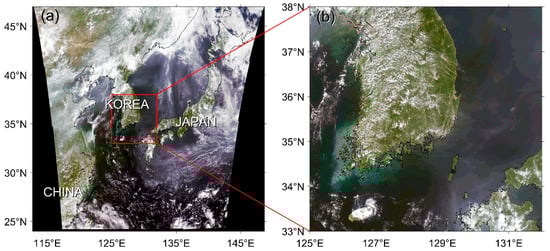
Figure 1.
(a) Geostationary Ocean Color Imager (GOCI) red–green–blue (RGB) image of the research area on 13 August 2013, (b) enlarged image of red box in (a).
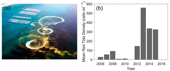
Figure 2.
(a) Red tide prevention work creating turbulence and spreading yellow soil on red tide on the southern coast of Korea (National Institute of Fisheries Science, NIFS); (b) annual mean red tide density from 2006 to 2016 (source: NIFS red tide report).
Most of the satellite remote sensing methods of red tide species have used near-polar orbiting satellites such as SeaWiFS, MODIS, and Landsat [5,27]. In the seas around the Korean Peninsula, the geostationary satellite Geostationary Ocean Color Imager (GOCI) has beneficially provided hourly observations and high spatial resolution of about 500 m over 10 years since 2010 [33,34]. A common challenge is posed by variation in local conditions. The seas surrounding the Korean Peninsula (Figure 1b) comprise three different coastal regions: clear waters along the eastern coast with relatively deep water depths, high turbidity and strong tidal currents along the western coast, and the southern coast with many islands and complicated coastlines as well as cold coastal waters and fronts confronted with northeastward-flowing Tsushima Warm Current [35,36]. Due to such diverse environments, it has been difficult to detect red tides with high accuracy and a standardized reproducible detection method for red tides is urgently needed.
This study aims to improve capacity in monitoring red tide events using GOCI in seas around the Korean Peninsula, and, in future applications, other regions worldwide. Specifically, our goals are to (1) evaluate the previous red tide detection methods applied to GOCI in Korean waters; (2) develop a new red tide index for GOCI data based on in situ spectral characteristics of the red tide and sea water; (3) compare the performance of existing and new methods; (4) validate the new red tide index with in situ measurements of cell densities, and (5) suggest a formulation to derive red tide cell density through the relation between density and the red tide index.
2. Data
2.1. Satellite Data
GOCI, onboard the Communication, Ocean and Meteorological Satellite (COMS), has observed the seas around the Korean Peninsula (24.75°N–47.25°N, 113.40°E–146.60°E) including the seas adjacent to China, Japan, Taiwan, and Russia with 500 m × 500 m spatial resolution and a high temporal sampling capability of 8 times per day from 9:00 a.m. to 4:00 p.m. (KST, Korean Standard Time) since June 2010 (Figure 1a). It has six visible (412, 443, 490, 555, 660, and 680 nm) and two near-infrared (NIR) channels (745 and 865 nm) with a bandwidth of 20 nm. For this study, 1440 images of level 2 atmospherically corrected [37] remote sensing reflectance (Rrs) (Version 2.0) from the Korea Ocean Satellite Center (KOSC) were utilized from 2012 to 2015. Unprecedented severe red tide events appeared in the southern and eastern coasts along the Korean Peninsula and offshore regions in the East Sea in 2013. Among hourly GOCI images on 13 August 2013, we selected an image with less cloudy conditions at a time of 04 UTC (local time, 1PM).
2.2. Spectroradiometer Measurements
In order to collect and understand spectral characteristics of red tides as a function of wavelength, we conducted cruise campaigns to collect in situ spectral measurements-water leaving radiance (LwT(λ)), sky radiance (Lsky(λ)), and irradiance (Ed(λ))-to calculate Rrs(λ) and match its values with satellite observed reflectances (Lsat(λ)) [38,39,40], along the southern coast of the Korean Peninsula during the red tide period from 2013 to 2015 on 8 August 2013 and 13 August 2015 (Figure 3). To develop the algorithm for red tide detection, it is indispensable to collect a wide spectrum of red tide characteristics. At the same time, it is also important to obtain spectral measurements from reference conditions, such as normal sea waters with chlorophyll-a concentration, suspended particulate matter (SPM), CDOM within normal ranges. The algorithm for red tide detection can be constructed by identifying peculiar characteristics, distinct from the usual sea water spectrum. Therefore, we collected the spectral reflectance of both turbid and clear waters when red tide did not appear during a period between 2013 to 2015.
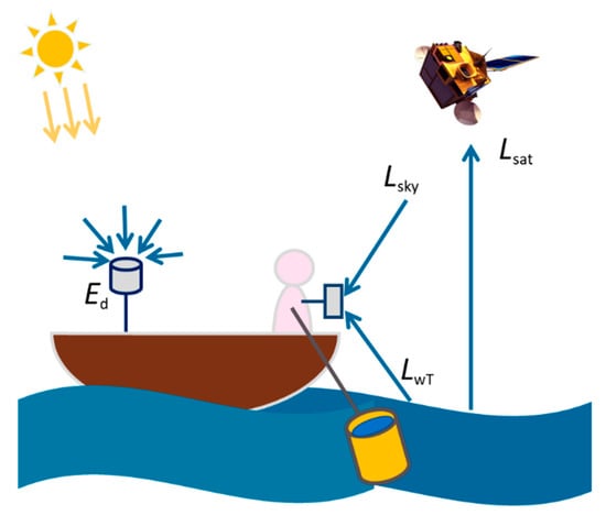
Figure 3.
Schematic diagram of on-board measurement procedures for water leaving radiance (LwT), sky radiance (Lsky), irradiance (Ed), and satellite-observed radiance (Lsat).
Spectral characteristics of seawater can strongly reflect its physical and biological state [41]. Figure 4 shows the bin-averaged distribution of Rrs against wavelengths, estimated from in situ spectral measurements for the red tides in 2013 and 2015, turbid waters, and clear sea waters. The bars represent the mean errors of Rrs values in each bin of wavelength. For example, clear water (blue lines in Figure 4) shows a decreasing Rrs at relatively shorter wavelengths of less than 600 nm and a relatively flat shape at higher wavelengths. Seawater with red tide clearly shows a different spectral shape, which reveals bimodal peaks at 560 and 680 nm (red and magenta lines in Figure 4). By contrast, spectral values corresponding to turbid water (green lines in Figure 4) show high values of about 0.008 sr−1 near 500–550 nm. All of these measurements were combined to derive a robust algorithm of red tide detection for GOCI data.
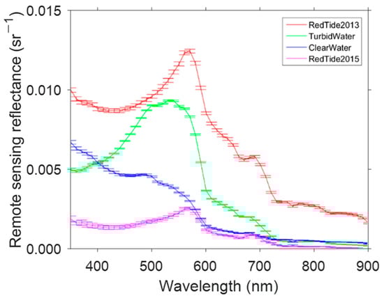
Figure 4.
In situ spectral remote sensing reflectances (Rrs) as a function of wavelength at the southern coast of the Korean Peninsula, where red and magenta-colored Rrs represent red tide water in 2013 and 2015, respectively, and green and blue lines represent the Rrs of turbid water and clear water, respectively. The upper and lower limits of the bars stand for the range of mean errors of Rrs with 1 standard errors at each wavelength.
2.3. In Situ Water Sampling and Analysis of Red Tide Species
To identify the red tide species and estimate the red tide density in the study area, we collected water samples in the southern coastal region of the Korean Peninsula on 8 August 2013 and 11 August 2014 during red tide events. We also sampled the sea water on 27 October 2013 during normal conditions after the disappearance of the red tides. To filter out the impact of chlorophyll-a concentration and SPM, we also estimated the two concentrations to be applied to derive the red tide density during the cruise periods [42,43]. Sample analysis showed that the main species of the red tides, comprising over 5 percent, are Skeletonema costatum, Cochlodinium polykrikoides, Pseudonitzschia species, and Thalassiosira species in the coastal region [5].
2.4. In Situ Red Tide Observation
To quantify the spatial distribution and density of the red tide species, we used reports from the National Institute of Fisheries Science (NIFS) about red tide events in Korea. The reports have been produced on a daily basis since 2006 (http://www.nifs.go.kr/redtideInfo) and contain information about the locations of red tide appearance acquired through ship cruises, aircraft, and observations on land as well as a range of red tide density by analyzing the sample sea water with vast red tide abundance [44]. Figure 5 shows an example of the digitalized map of the daily red tide report from NIFS. Red circular or elliptic patterns indicate the locations where red tide was observed during the ship cruise surveys.
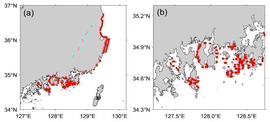
Figure 5.
(a) Red tide report map and (b) enlarged southern coastal area of (a) on 13 August 2013 (source: National Institute of Fisheries Science), where the red-colored areas indicate the places where red tide events were observed.
3. Methods
To compare the previously developed methods and the method from this study, we selected five different red-tide detection algorithms such as Band Ratio Index (BRI), MODIS Red tide Index (MRI), Red tide Index (RI), and alternative index using Fluorescence Line Height (FLH) [30,31,45,46,47,48,49]. The performance of these algorithms is investigated by applying them to GOCI data, and then comparing with the newly developed algorithm from this study, called the Normalized Red Tide Index (NRTI).
3.1. Previous Methods of Red Tide Detection
Among previous red tide indices, we chose 4 representative indices to test if the algorithms are applicable to GOCI data. Since most of the following methods have been developed for different near-polar orbiting satellites such as SeaWiFS and MODIS, we selected GOCI band data with wavelengths closest to the band of each satellite for the calculation of the following red tide index.
3.1.1. Band Ratio Index (BRI)
The Band Ratio Index (BRI) uses three visible channels of SeaWiFS designed for red tide in the Northwestern Pacific Ocean including seas around the Korean Peninsula [46]. The BRI is a ratio composed of the three bands as follows:
where (λ) is water leaving radiance and is coefficient. The BRI value is close to 1, which means a stronger red tide occurred. In the beginning stages of red tide monitoring using GOCI data, the KOSC tried to distribute the red tide data by modifying the coefficient and channels for GOCI as a level-3 parameter in the GOCI data processing system. Due to lack of 510 in GOCI, 510 was replaced with and the coefficient is assigned to 0.375 [50].
3.1.2. Fluorescence Line Height (FLH)
Fluorescence Line Height (FLH, mW cm−2 µm−1 sr−1) is the height of the spectral peak of normalized water leaving radiance ( over near infrared, which can be expressed by three channels of 667, 678, and 748 nm [45,47]:
As one of the ocean color products from NASA, the FLH has been used for estimating HAB distribution in several different seas and species. The FLH method was utilized for surveying Karenia brevis in the Gulf of Mexico and multiple species in Monterey Bay using MODIS [31,45]. However, GOCI has different near infrared channels from MODIS. Therefore, we replaced the 667, 678, 748 values with 660, 680, 745, respectively, for comparisons with the algorithm from the present study.
3.1.3. MODIS Red Tide Index (MRI)
Using two visible channels of MODIS, the MODIS Red tide Index (MRI) was suggested as a procedure to discern red tide areas occurring along the coast of Korea [48]. The MRI is defined as a ratio of the difference between and to their sum:
A positive MRI index indicates that red tides have occurred. To apply the MRI to GOCI data, we employed and instead of the and of MODIS. Then, two additional steps were implemented by specifying the thresholds of SST and turbid areas. As the first limit of SST variations, the pixels of sea water with SSTs outside the range of 22–26 °C were discarded. Additionally, turbid regions were excluded from the red tide detection by employing the threshold of (>0.15). Using the formulation of (3), the MRI was estimated to compare the spatial distribution of the detected red tide using GOCI data with that of other methods.
3.1.4. Red Tide Index (RI)
Using three visible channels ( of GOCI, Red tide index (RI) was suggested in the East China Sea where the red tide species of Prorocentrum donghaiense are abundant [30]. The RI has the following formulation:
A negative RI value indicates that the status of sea water is normal and without red tide. When RI is greater than 2.2 (4.0) at a certain region, sea water of the region was considered to contain red tide. RI amounting to over 4.0 implies that red tide with an extremely high density exists. The result of the derived RI was also compared with that of other methods.
3.2. Development of a New Normalized Red Tide Intensity Index (NRTI)
A novel Red tide intensity index was calculated based on in situ spectral measurements. In situ spectral measurements indicated peculiar spectral shapes of the red tide with bimodal peaks at 550 and 680 nm, marked in red and magenta lines in Figure 4, as compared with those of normal sea water. Such peaks are induced by the strengthened absorption of solar insolation by red tide and change in fluorescence [1,49,51]. This implies a relation between red tide density and the heights of the peaks. As red tide density increases, so does the kurtosis of each peak. Considering the available channels of GOCI, the Rrs of the red tide can be characterized by selecting the two distinct peaks at 555 nm and 680 nm in spectral reflectance as shown in Figure 6. Based on the spectral characteristics of red tides, we designed a new Red Tide Intensity (RTI) index for GOCI data. The basic index was composed of the multiplication of the two peak heights from the linear lines between the reflectances of two adjacent bands at the center of the main bands (555 and 680 nm) (Figure 6):
where P555 (P680) represents the first (second) peak height. Considering that ranges are different by atmospheric correction scheme and satellite sensors, we contrived additional step as a kind of normalization:
where NRTI refers to normalized RTI.
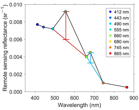
Figure 6.
Spectral distribution of remote sensing reflectance with bimodal peaks at GOCI spectral bands from 412 to 865 nm, where red and blue lines show how to calculate the bimodal peak heights in the red tide index algorithm.
Before applying the NRTI to GOCI, speckles in the GOCI images were first removed by using data on SPM [34] and then calculated chlorophyll-a concentration [52,53] using a 3-band ocean color algorithm (called OC3 algorithm) (Figure 7). Pixels with negative values of were regarded as failures of atmospheric correction and replaced with NaN values. At each step of the peak height calculation, of three consecutive channels were used as shown in (5) and (6). Pixels with negative values of P555 and P680 were regarded as red tide free. To adjust and mitigate the heights of both peaks, the peak height is designed to be normalized by dividing with of the shortest wavelength among the three channels in each peak. In clear water, the values of P555 and P680 can be potentially extremely high by being divided by too small of a denominator. To avoid this situation, we assumed small values of and as 0.01 and 0.001, only if the values are smaller than 0.01(Th1) and 0.001(Th2), respectively (Figure 7).
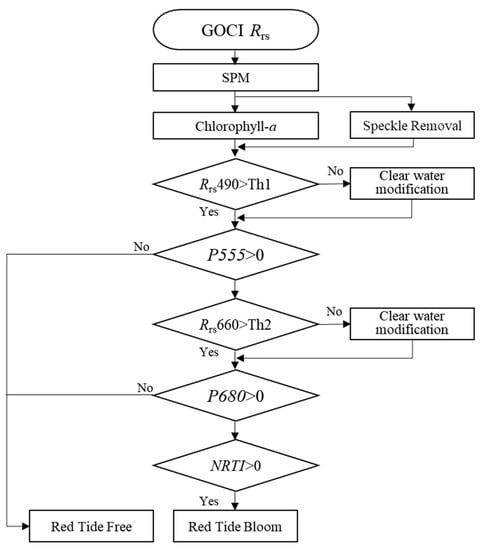
Figure 7.
Flow chart of red tide detection procedures including preprocessing of data (, remote sensing reflectance) quality control, calculating each peak (P555 and P680), and determining the existence of a red tide bloom (Th1 and Th2 are thresholds).
4. Results
4.1. Inter-Comparison of Previous Methods
Prior to the comparison of a presently developed method with other methods, four representative methods of red tide detection were investigated to determine if they accurately captured the spatial distribution and intensity of the red tides.
4.1.1. Band Ratio Index (BRI)
The estimated values of BRI using GOCI data ranged from −1 to 1 in the seas around the Korean Peninsula (Figure 8a). The spatial distribution of modified BRI values shows the lowest indices of less than −0.2 in the southwestern coastal region. In contrast, the eastern coastal, as well as offshore region (36°N–37N°), indicate a relatively high BRI of greater than 0.5, with extremely high BRI (>0.9) as an indicator of the occurrence of distinctive red tides. The most and least abundant red tide event occurring areas are matched with in situ observation (Figure 5a); however, there are some areas showing discrepancies. One of the most distinctive discrepancies is found in most of the southwestern offshore regions in the East Sea where the BRI values are below zero. This method failed to detect the red tide events that occurred in the southwestern region off of the Korean Peninsula. As shown in Figure 5a, however, an extremely high red tide concentration occurred along the southeastern coast of the Korean Peninsula. Another noticeable feature is the relatively high BRI values, over 0.3, in the nearshore regions along the eastern coastline. In contrast to this result, red tides were not reported in the northern part of the study area. In light of these results, the BRI is not suitable for monitoring the red tide using GOCI data.
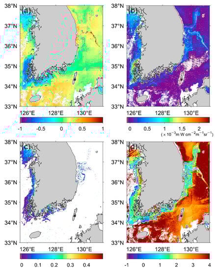
Figure 8.
Spatial distribution of the red tide index as a result of applying previous methods of (a) BRI, (b) FLH (mW cm−2 µm−1 sr−1), (c) MRI, and (d) RI to a GOCI image (04 UTC, 13 August 2013).
4.1.2. Fluorescence Line Height (FLH)
The spatial distribution of the FLH values ranged from 0 to 2.5 × 10⁻³ mW cm−2 µm−1 sr−1 as shown in Figure 8b. Most of the coastal regions presented relatively high values (>0.8 × 10⁻³ mW cm−2 µm−1 sr−1) than those of offshore regions. Differently from BRI, low FLH offshore makes broad red tide patterns more recognizable. The FLH method shows the strengthening of the red tide in the coastal region. However, the highest FLH values are along the southwestern coast of Korea in the Yellow Sea, where the red tide event was not reported during summer 2013. This region is known for highly turbid water with abundant SPM due to strong tidal currents and dominant vertical mixing at shallow water depths. This result shows a reverse tendency, compared to the BRI index in the southwestern coastal area. Considering the tendency, FLH is needed to be used in the turbid water before being utilized for red tide monitoring in Korean water.
4.1.3. MODIS Red Tide Index (MRI)
Most MRI values are close to zero in the offshore region except for the western coast of the Yellow Sea and the southwestern coasts of the Korean Peninsula (Figure 8c). MRIs of less than 0.2 in the western side coincide with highly turbid waters. This suggests a need to remove the effect of the SPM in the quality control process. However, without the highly turbid areas, the MRI shows negative values in the most of red tide event observed areas. When we applied the turbid water removal threshold of (>0.15) directly to GOCI [48], most regions were eliminated (Figure 8c shows MRI before applying the threshold). It could be due to the instrumental characteristics of each of the satellite sensors, so we decided not to apply turbid water removal process to MRI calculation to investigate its overall spatial pattern. Relatively high values (>0.2) in the East Sea are not detected along the coast, but rather in the offshore regions (36°N–37°N). In contrast to these MRI values, the southwestern coast does not show any signs of red tide. The MRI shows even negative values in the southern part of the east coast, inconsistent with the observed red tide density on that day. Such differences probably originate from different satellite sensors and spectral bands. Thus, the MRI index is not likely to be applicable to the GOCI data directly as a representative formulation for red tide monitoring in Korean waters.
4.1.4. Red Tide Index (RI)
The application of RI to Korean waters shows clear differences between nearshore (<2) and offshore (>2) regions. Figure 8d shows the estimated RI developed for the East China Sea using GOCI images according to the algorithm of [30]. However, the overall distribution of the RI exhibits reverse trends opposite to the known features. Results show that most of the inner nearshore regions have no relation to the red tide event. Only a few areas of the coastal regions have RI values greater than 3, corresponding to the red tide appearance, in the coastal regions near 36°N in the East Sea and in the southern coastal region around 127°E. Most of the coastal area ranged from 0 to 2 (blue-green), indicating that RI is also not suitable for the detection of red tides in this region. Application of these existing red tide detection algorithms reveals persistent inconsistencies for GOCI images, indicating that other methods should be developed for the red tide monitoring as well as for the quantification of red tide intensity using the GOCI data.
4.2. Estimation of Normalized Red Tide Index
Based on in situ measurements by NIFS, the red tide was reported to appear in coastal regions along the central portion of the southeastern coast and the eastern coast up to 37°N, with a maximum cell density ranging from 1020 to 20,000 cells mL−1 on August 13, 2020 (Figure 9a). Since the in situ observations had been conducted only in the coastal regions, the red tide map should be carefully interpreted in that it did not carry the information on the existence of the red tides in the offshore region far from the coastline. At 36°N of the eastern coast, red tide density amounted to the highest value of about 20,000 cells mL−1 as denoted in red in Figure 9a. The second highest value was found near Geoje Island in the southern coast (34.8°N, 128.7°E, orange color in Figure 9a) with 17,280 cells mL−1.
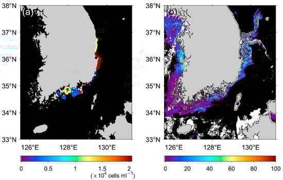
Figure 9.
(a) Digitized red tide report map with highest density (cells mL−1) and (b) NRTI map on 13 August 2013.
The NRTI method was applied to detect red tide using GOCI level-2 Rrs data (GDPS v2.0) on 13 August 2013. Most of the offshore regions were not associated with the occurrence of red tide. The black colored region indicates NaN values in Figure 9b. When focusing on the sites with in situ measurements (Figure 9a), with the visual exaggeration of the observed red tide at the in situ stations in terms of spatial coverage, the highest value of red tide density was detected along the eastern coast (36°N–37°N). The NRTI map revealed concordance with the in situ measurements, i.e., by showing the highest value along the eastern coast (36°N–37°N), the lowest value in the southwestern coast, and a very low index free of red tide in the offshore region (Figure 9b–c). In contrast with limitations of the previous methods in describing the spatial distributions of the red tide event, the present index seems to adequately capture its spatial distribution, as well as the intensity. Detailed relations between the NRTI and red tide density are depicted in the following section.
4.3. Retrieval of Red Tide Density
NRTI values tend to increase with red tide intensity, which suggests a high possibility to derive red tide cell density or red tide concentration from satellite-observed NRTI. Therefore, we first investigated the relationship between red tide concentration and the red tide index. As shown in Figure 10, there is a significant positive relationship between red tide density (RTD) and the NRTI values (p-value < 10−10 with 95% confidence interval). The relationship can be expressed by the following linear function:
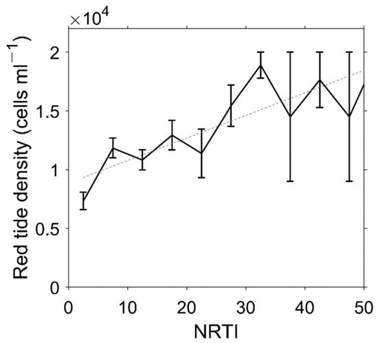
Figure 10.
Variations of in situ red tide density as a function of NRTI at the in situ red tide occurring region (04 UTC, 13 August 2013). Solid line represents the mean and standard error of red tide density within each NRTI bin. Dashed line indicates linear regression between NRTI and red tide density Equation (9).
The Root Mean Square (RMS) error and bias between the regressed values and the in situ red tide density are estimated at 2060 and −0.6913 cells mL−1 with R2 value of 0.7569, respectively. The probability of detection (POD) values of the red tide detection amounted to 0.7068. The zero NRTI values indicate that the sea water would contain no red tide species. Accordingly, the linear regression formulation reflects absorption of red tide species with the deviation from the normal spectrum as compared with the spectra at adjacent bands.
During the red tide events, chlorophyll-a concentration values from satellite data are generally greater than those of normal sea water. Figure 11a presents the spatial distribution of the GOCI chlorophyll-a concentration using a three-band ocean color algorithm (called OC3 algorithm). Most of the coastal regions along the Korean Peninsula showed higher chlorophyll-a values over 0.2 log10 mg m−3 than those of offshore regions. Most of the previous methods (FLH, MRI, RI) produced relatively high red tides, especially in the southwestern coastal region and at 04 UTC on 13 August 2013 (Figure 8). However, this is not coincident with in situ field observations. According to the in situ measurements by NIFS, there were no red tides at the southern part of the western coast and the southern coast (34°N–35°N, 125.5°E–127.0°E) at that time. Since NIFS started monitoring red tides, red tides have been rarely reported in this region with strong tidal currents and turbulence [36].
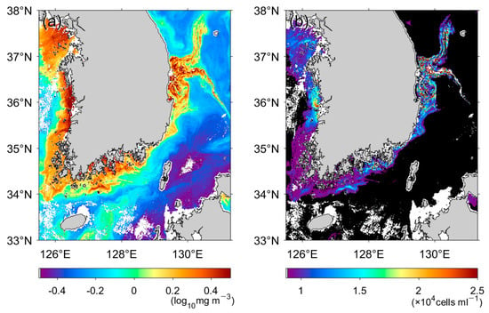
Figure 11.
(a) Chlorophyll-a concentration (log10 mgm−3, OC3 algorithm), (b) estimated red tide density using NRTI (04 UTC, 13 August 2013).
Since the western coast has high SPM concentration induced by strong tidal mixing and current over shallow bathymetry, it was very difficult to detect red tide in turbid waters. On the other hand, the red tide index as well as red tide density (Figure 11b), retrieved by the new NRTI method, reproduce the red tide concentration satisfactorily along the southern and eastern coasts up to 37°N. In particular, extremely high red tide concentrations at a range from 15,000 to 25,000 cells mL−1 were well captured by NRTI in the East Sea, showing two branches stretching to the offshore region. The highest concentration of in situ observed red tide density was about 20,000 cells mL−1 and appeared at 36°N along the eastern coast near the coastlines. This was remarkably coincident with the actual observations. Therefore, it is expected that the present method of this study will be able to detect red tide with much better performance than other conventional methods. Furthermore, the study is notable in that it suggests a method to calculate the density of red tide that has never been tried before.
4.4. Retrieval Formulation of Red Tide Density
In the previous section, this study illustrated a relationship between NRTI and the red tide density from 2012 to 2015. Figure 12 shows the red tide density with respect to the estimated NRTI. Although mean error bars tend to increase as NRTI increases, overall distribution reveals a linear relationship of the red tide density to the NRTI as follows (p-value < 10−43 within 95% confidence interval)
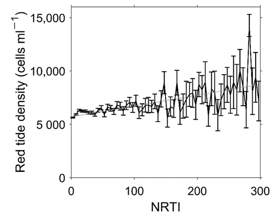
Figure 12.
Variations of in situ red tide density (cells mL−1) as a function of NRTI at the matchup locations between satellite data and in situ measurements of red tide from 2012 to 2015, where the dashed line represents the least-squared linear fit between the NRTI and the red tide density, and the bars of each bin represent the mean errors expressed as the upper and lower limits of the 1 standard error of the in situ red tide density.
The RMS error and bias between the regressed values and the in situ red tide density are estimated to 1118 and 0.1421 cells mL−1 with R2 value of about 0.3882, respectively. The POD values of the observation amounted to 0.7637. It is noted that the calculated NRTI can represent the red tide density. This implies that we can estimate the red tide concentration, similar to the chlorophyll-a concentration formulation if the red tide index is calculated from the equation we suggested in this study.
5. Discussion
The newly developed red tide index (NRTI) shows high correlation with in situ red tide observation in spatial distribution as well as its density in various conditions of local seas around the Korean Peninsula, which enables us to provide detailed spatial structure of the red tide abundance despite the offshore location, which is logistically time consuming and costly to monitor. In the case of the lack of in situ measurements, the NRTI can fill the spatial data gap with high accuracy.
Utilizing previous algorithms developed for other satellites or different waters to GOCI and Korean waters has several potential shortcomings. Due to different spectral characteristics of satellite sensors, the coefficients of the present formulation of red tide density in this study are not expected to be directly used for other sensor data. In case of chlorophyll-a concentration, many of the algorithms have diverse formulations and different coefficients such as the ocean color algorithm (OCx). In addition, atmospheric correction procedure can produce change in reflectance at each band. In case of GOCI, reflectance values by Versions 1.3 and 2.0 of the atmospheric correction schemes show a significantly different range of reflectances. V1.3 produced much higher values than V2.0 according to our investigations, which induced the different heights of the spectral peaks. To avoid such differences, this study considered the effect of atmospheric correction difference in the normalization procedure. The present results suggest a possibility that the formulation of the NRTI method can be utilized as one of the representative red tide detection methods for other ocean color satellites as well.
Although spectral bimodal peaks are typical characteristics of red tide species, considering that different species have different cell volume or pigment amount, the red tide cell density algorithm should be further retrieved by species or cell size. However, in the seas in this study, C. polykrikoides has been one of the most dominant species of the red tide blooms over a long period in the seas around Korea [32,44,54]. Dominance by this species likely underlies the strong positive relationship we found between NRTI and cell density. Repeated dominance of this species in Korean waters suggests this index can effectively describe other red tide events in Korean waters.
The southwestern coast of the Korean Peninsula, characterized by high turbidity and SPM, is one of the most difficult regions for the estimation of red tides as shown in Figure 1b. In estimation of chlorophyll-a concentration and red tide density, the SPM can be an obstacle since high SPM increases reflectance of sea water. To remove the effect of high SPM, we normalized peak heights with the reflectance with the shortest wavelength during the NRTI calculation procedure. The present result in Figure 11b reveals its high potential to the application of the strong tidal mixing zone in the Yellow Sea as well as the southern coastal regions off the Korean Peninsula, and similarly turbid waters in other regions. Most of the previous methods have failed to discriminate the red tide under highly turbid conditions. However, this formulation produced very low values of less than 10,000 cells mL−1 in spite of the high SPM in the strong tidal mixing zone. This implies that the present method can enhance the capability of red tide detection by overcoming the shortcomings of the existing methods.
One of the important specific questions raised is whether the high red tide density, with relatively high concentration exceeding 2.2 × 10⁴ cells mL−1 in the middle of western coast around 36°N and 126°E in the Yellow Sea, is a realistic estimate. This region has relatively small tidal currents compared to the region off the southwestern corner of the Korean Peninsula, but it still has a medium range of SPM in shallow bathymetry. The report of NIFS on the red tide distribution confirmed the occurrence of red tides in the region as shown in Figure 11b. The comparison of the present NRTI method showed a good correlation with a positive relationship to in situ red tide density in terms of spatial distribution in the coastal region of the Yellow Sea. According to the NIFS reports published in 2013, the red tide species called C. polykrikoides was observed along the western coast. This report supports the reasonable feasibility of the estimated NRTI and red tide density in Figure 11b. To validate the red tide density along the western coast quantitatively, more continuously collected in situ measurements will be needed. Most of the in situ observations are concentrated along the southern and eastern coasts as a priority due to previous large-scale damage to fishing farms by red tides. Previous NIFS reports have already mentioned the sporadic appearance of the red tides at the western coast of Korea in other years. More sampling works along the western coast are needed to improve our understanding of the red tide features.
6. Conclusions
During severe red tide events, spectral characteristics of the red tide were investigated through in situ spectroradiometer observations in the seas around the Korean Peninsula. Inter-comparisons of previous representative methods for red tide detection reveal limitations for GOCI data in the study area. Methods such as BRI, FLH, MRI, and RI show discrepancies with in situ red tide observation data in spatial distribution. Moreover, the previous index has not been used for the estimation of red tide concentration. A new method of red tide detection is suggested by developing a red tide index that uses geostationary ocean color satellite data and in situ observations. The newly developed NRTI index is based on bimodal peaks in spectral characteristics at wavelengths from visible to NIR. The results applied to GOCI data show good performance in red tide detection in normal oceanic conditions as well as in highly turbid conditions over shallow bathymetry. Importantly, this study identified a strong relationship with red tide cell density by regressing the GOCI-based red tide index data to in situ red tide density. The estimated density showed good agreement with the observed density, with a linear relation and relatively small RMS and bias errors.
The NRTI has the potential to be broadly applicable to detecting red tide events and estimating red tide density from diverse satellite data. An open question is whether the present formulation can be applied to other seas and other satellites. However, we anticipate that the fundamental concepts of the NRTI could be adapted and extensively utilized for near-real time monitoring of red tide events. In addition to the NRTI, the red tide density formulation can be applied to other coastal regions in other local seas and the global ocean.
The seas around the Korean Peninsula have been highly utilized for aquaculture and fisheries, but they frequently suffer from severe red tide events. Although the NIFS has monitored red tide outbreaks, most of the in situ monitoring and surveillance has been highly focused on nearshore regions due to high costs and effort. Once the reflectance values of each satellite observation are obtained, it is possible that the present method can be easily and reliably applied for real-time monitoring of red tides and estimation of red tide cell density. In light of this, we anticipate that this red-tide monitoring method could enable efficient management of fishery resources and mitigation of economic disasters in many other coastal regions around the world.
Author Contributions
Conceptualization, K.-A.P.; data curation, M.-S.L.; methodology, M.-S.L. and K.-A.P.; writing–original draft preparation, M.-S.L.; writing–review and editing; K.-A.P. and F.M. All authors have read and agreed to the published version of the manuscript.
Funding
This research was a part of the project titled “Long-term change of structure and function in marine ecosystems of Korea” (1525009695) and “Deep Water Circulation and Material Cycling in the East Sea” (1525010256) funded by the Ministry of Oceans and Fisheries, Korea. This research was also supported by National Science Foundation (#1736830) and the Gilbert Morgan Smith Memorial Fund.
Informed Consent Statement
Not applicable
Data Availability Statement
All data used in this study are available from NIFS (red tide report data, http://www.nifs.go.kr/redtideInfo) or KOSC (GOCI satellite data, http://kosc.kiost.ac.kr/).
Acknowledgments
We thank the National Institute of Fisheries Science for the red tide monitoring report. We thank the Korea Ocean Satellite Center for the GOCI satellite data. We thank Geoview and S.E.O.U.L. for help with field data collections. We also thank J. Lee and C. Butner for helpful comments on the manuscript.
Conflicts of Interest
The authors declare no conflict of interest.
References
- Kahru, M.; Mitchell, B.G. Spectral reflectance and absorption of a massive red tide off southern California. J. Geophys. Res. Ocean. 1998, 103, 21601–21609. [Google Scholar] [CrossRef]
- Walsh, J.J.; Jolliff, J.; Darrow, B.; Lenes, J.; Milroy, S.; Remsen, A.; Dieterle, D.; Carder, K.L.; Chen, F.; Vargo, G.A. Red tides in the Gulf of Mexico: Where, when, and why? J. Geophys. Res. Ocean. 2006, 111, 1–46. [Google Scholar] [CrossRef] [PubMed]
- He, R.; McGillicuddy, D.J., Jr.; Keafer, B.A.; Anderson, D.M. Historic 2005 toxic bloom of Alexandrium fundyense in the western Gulf of Maine: 2. Coupled biophysical numerical modeling. J. Geophys. Res. Ocean. 2008, 113, 1–12. [Google Scholar]
- Jessup, D.A.; Miller, M.A.; Ryan, J.P.; Nevins, H.M.; Kerkering, H.A.; Mekebri, A.; Crane, D.B.; Johnson, T.A.; Kudela, R.M. Mass stranding of marine birds caused by a surfactant-producing red tide. PLoS ONE 2009, 4, e4550. [Google Scholar] [CrossRef] [PubMed]
- Lee, M.-S.; Park, K.-A.; Chae, J.; Park, J.-E.; Lee, J.-S.; Lee, J.-H. Red tide detection using deep learning and high-spatial resolution optical satellite imagery. Int. J. Remote Sens. 2020, 41, 5838–5860. [Google Scholar] [CrossRef]
- Anderson, D.M.; Cembella, A.D.; Hallegraeff, G.M. Progress in understanding harmful algal blooms: Paradigm shifts and new technologies for research, monitoring, and management. Annu. Rev. Mar. Sci. 2012, 4, 143–176. [Google Scholar] [CrossRef]
- Brunson, J.K.; McKinnie, S.M.; Chekan, J.R.; McCrow, J.P.; Miles, Z.D.; Bertrand, E.M.; Bielinski, V.A.; Luhavaya, H.; Oborník, M.; Smith, G.J. Biosynthesis of the neurotoxin domoic acid in a bloom-forming diatom. Science 2018, 361, 1356–1358. [Google Scholar] [CrossRef]
- Wells, M.L.; Trainer, V.L.; Smayda, T.J.; Karlson, B.S.; Trick, C.G.; Kudela, R.M.; Ishikawa, A.; Bernard, S.; Wulff, A.; Anderson, D.M. Harmful algal blooms and climate change: Learning from the past and present to forecast the future. Harmful Algae 2015, 49, 68–93. [Google Scholar] [CrossRef]
- McKibben, S.M.; Peterson, W.; Wood, A.M.; Trainer, V.L.; Hunter, M.; White, A.E. Climatic regulation of the neurotoxin domoic acid. Proc. Natl. Acad. Sci. USA 2017, 114, 239–244. [Google Scholar] [CrossRef]
- Gobler, C.J.; Doherty, O.M.; Hattenrath-Lehmann, T.K.; Griffith, A.W.; Kang, Y.; Litaker, R.W. Ocean warming since 1982 has expanded the niche of toxic algal blooms in the North Atlantic and North Pacific oceans. Proc. Natl. Acad. Sci. USA 2017, 114, 4975–4980. [Google Scholar] [CrossRef]
- Schantz, E.J. Poisonous red tide organisms. Environ. Lett. 1975, 9, 225–237. [Google Scholar] [CrossRef] [PubMed]
- Anderson, D.M. Toxic algal blooms and red tides: A global perspective. In Red Tides: Biology, Environmental Science and Toxicology; Elsevier: New York, NY, USA, 1989; pp. 11–16. [Google Scholar]
- Hallegraeff, G.M. A review of harmful algal blooms and their apparent global increase. Phycologia 1993, 32, 79–99. [Google Scholar] [CrossRef]
- Lu, S.; Hodgkiss, I. Harmful Algal Bloom Causative Collected from Hong Kong Waters, in Asian Pacific Phycology in the 21st Century: Prospects and Challenges; Springer: Berlin, Germany, 2004; pp. 231–238. [Google Scholar]
- MacIntyre, J.G.; Cullen, J.J.; Cembella, A.D. Vertical migration, nutrition and toxicity in the dinoflagellate Alexandrium tamarense. Mar. Ecol. Prog. Ser. 1997, 148, 201–216. [Google Scholar] [CrossRef]
- Anderson, D.M.; White, A.W.; Baden, D.G. Toxic Dinoflagellates; Elsevier: New York, NY, USA, 1985. [Google Scholar]
- Anderson, D.M.; Glibert, P.M.; Burkholder, J.M. Harmful algal blooms and eutrophication: Nutrient sources, composition, and consequences. Estuaries 2002, 25, 704–726. [Google Scholar] [CrossRef]
- Gravinese, P.M.; Munley, M.K.; Kahmann, G.; Cole, C.; Lovko, V.; Blum, P.; Pierce, R. The effects of prolonged exposure to hypoxia and Florida red tide (Karenia brevis) on the survival and activity of stone crabs. Harmful Algae 2020, 98, 101897. [Google Scholar] [CrossRef]
- Stumpf, R.P.; Tomlinson, M.C.; Calkins, J.A.; Kirkpatrick, B.; Fisher, K.; Nierenberg, K.; Currier, R.; Wynne, T.T. Skill assessment for an operational algal bloom forecast system. J. Mar. Syst. 2009, 76, 151–161. [Google Scholar] [CrossRef]
- McGillicuddy, D., Jr. Models of harmful algal blooms: Conceptual, empirical, and numerical approaches. J. Mar. Syst. 2010, 83, 105. [Google Scholar] [CrossRef]
- Heisler, J.; Glibert, P.M.; Burkholder, J.M.; Anderson, D.M.; Cochlan, W.; Dennison, W.C.; Dortch, Q.; Gobler, C.J.; Heil, C.A.; Humphries, E. Eutrophication and harmful algal blooms: A scientific consensus. Harmful Algae 2008, 8, 3–13. [Google Scholar] [CrossRef]
- Anderson, D.M.; Burkholder, J.M.; Cochlan, W.P.; Glibert, P.M.; Gobler, C.J.; Heil, C.A.; Kudela, R.M.; Parsons, M.L.; Rensel, J.J.; Townsend, D.W. Harmful algal blooms and eutrophication: Examining linkages from selected coastal regions of the United States. Harmful Algae 2008, 8, 39–53. [Google Scholar] [CrossRef]
- Weisberg, R.H.; Liu, Y.; Lembke, C.; Hu, C.; Hubbard, K.; Garrett, M. The coastal ocean circulation influence on the 2018 West Florida Shelf K. brevis red tide bloom. J. Geophys. Res. Ocean. 2019, 124, 2501–2512. [Google Scholar] [CrossRef]
- Granéli, E.; Turner, J.T. Ecology of Harmful Algae; Springer: Berlin, Germany, 2006; Volume 189. [Google Scholar]
- Anderson, D. HABs in a changing world: A perspective on harmful algal blooms, their impacts, and research and management in a dynamic era of climactic and environmental change. In Harmful algae 2012: Proceedings of the 15th International Conference on Harmful Algae: October 29–November 2, 2012, CECO, Changwon, Gyeongnam, Korea/editors, Hak Gyoon Kim, Beatriz Reguera, Gustaaf M. Hallegraeff, Chang. Kyu Lee, M.; NIH Public Access: Bethesda, MD, USA, 2014. [Google Scholar]
- Carder, K.; Steward, R. A remote-sensing reflectance model of a red-tide dinoflagellate off west Florida 1. Limnol. Oceanogr. 1985, 30, 286–298. [Google Scholar] [CrossRef]
- Stumpf, R.; Culver, M.; Tester, P.; Tomlinson, M.; Kirkpatrick, G.; Pederson, B.; Truby, E.; Ransibrahmanakul, V.; Soracco, M. Monitoring Karenia brevis blooms in the Gulf of Mexico using satellite ocean color imagery and other data. Harmful Algae 2003, 2, 147–160. [Google Scholar] [CrossRef]
- Choi, J.-K.; Min, J.-E.; Noh, J.H.; Han, T.-H.; Yoon, S.; Park, Y.J.; Moon, J.-E.; Ahn, J.-H.; Ahn, S.M.; Park, J.-H. Harmful algal bloom (HAB) in the East Sea identified by the Geostationary Ocean Color Imager (GOCI). Harmful Algae 2014, 39, 295–302. [Google Scholar] [CrossRef]
- Frolov, S.; Kudela, R.M.; Bellingham, J.G. Monitoring of harmful algal blooms in the era of diminishing resources: A case study of the US West Coast. Harmful Algae 2013, 21, 1–12. [Google Scholar] [CrossRef]
- Lou, X.; Hu, C. Diurnal changes of a harmful algal bloom in the East China Sea: Observations from GOCI. Remote Sens. Environ. 2014, 140, 562–572. [Google Scholar] [CrossRef]
- Ryan, J.P.; Davis, C.O.; Tufillaro, N.B.; Kudela, R.M.; Gao, B.-C. Application of the hyperspectral imager for the coastal ocean to phytoplankton ecology studies in Monterey Bay, CA, USA. Remote Sens. 2014, 6, 1007–1025. [Google Scholar] [CrossRef]
- National Institute of Fisheries Science. Monitoring, Management and Mitigation of Red Tide; Annual report of NIFS on red tide of Korea; National Institute of Fisheries Science: Busan, Korea, 2019. [Google Scholar]
- Ryu, J.-H.; Han, H.-J.; Cho, S.; Park, Y.-J.; Ahn, Y.-H. Overview of geostationary ocean color imager (GOCI) and GOCI data processing system (GDPS). Ocean Sci. J. 2012, 47, 223–233. [Google Scholar] [CrossRef]
- Lee, M.-S.; Park, K.-A.; Moon, J.-E.; Kim, W.; Park, Y.-J. Spatial and temporal characteristics and removal methodology of suspended particulate matter speckles from Geostationary Ocean Color Imager data. Int. J. Remote Sens. 2019, 40, 3808–3834. [Google Scholar] [CrossRef]
- Moriyasu, S. The tsushima current. In Kuroshio: Its Physical Aspects; University of Tokyo Press: Tokyo, Japan, 1972; pp. 353–369. [Google Scholar]
- Park, K.-A.; Lee, M.-S.; Park, J.-E.; Ullman, D.; Cornillon, P.C.; Park, Y.-J. Surface currents from hourly variations of suspended particulate matter from Geostationary Ocean Color Imager data. Int. J. Remote Sens. 2018, 39, 1929–1949. [Google Scholar] [CrossRef]
- Ahn, J.-H.; Park, Y.-J.; Kim, W.; Lee, B. Simple aerosol correction technique based on the spectral relationships of the aerosol multiple-scattering reflectances for atmospheric correction over the oceans. Opt. Express 2016, 24, 29659–29669. [Google Scholar] [CrossRef]
- Ahn, Y.-H. Optical Properties of Biogenous and Mineral Particles Present in the Ocean. Application: Inversion of Reflectance. Ph.D. Thesis, Paris-VI University, Paris, France, 1990. [Google Scholar]
- Austin, R.W. The remote sensing of spectral radiance from below the ocean surface. In Opt. Asp. Oceanogr. Jerlov and Nielson (eds.); Academic Press: New York, NY, USA, 1974; pp. 317–344. [Google Scholar]
- Mobley, C.D. Estimation of the remote-sensing reflectance from above-surface measurements. Appl. Opt. 1999, 38, 7442–7455. [Google Scholar] [CrossRef] [PubMed]
- Robinson, I.S. Measuring the Oceans from Space: The Principles and Methods of Satellite Oceanography; Springer Praxis Publishing: Chichester, UK, 2004; pp. 178–184. [Google Scholar]
- Holm-Hansen, O.; Lorenzen, C.J.; Holmes, R.W.; Strickland, J.D. Fluorometric determination of chlorophyll. Ices J. Mar. Sci. 1965, 30, 3–15. [Google Scholar] [CrossRef]
- Lorenzen, C.J. Determination of chlorophyll and pheo-pigments: Spectrophotometric equations 1. Limnol. Oceanogr. 1967, 12, 343–346. [Google Scholar] [CrossRef]
- Lee, C.-K.; Park, T.-G.; Park, Y.-T.; Lim, W.-A. Monitoring and trends in harmful algal blooms and red tides in Korean coastal waters, with emphasis on Cochlodinium polykrikoides. Harmful Algae 2013, 30, S3–S14. [Google Scholar] [CrossRef]
- Abbott, M.R.; Letelier, R.M. Algorithm Theoretical Basis Document Chlorophyll Fluorescence (MODIS Product Number 20). NASA. Available online: https://modis.gsfc.nasa.gov/data/atbd/atbd_mod22.pdf (accessed on 1 September 2016).
- Ahn, Y.-H.; Shanmugam, P. Detecting the red tide algal blooms from satellite ocean color observations in optically complex Northeast-Asia Coastal waters. Remote Sens. Environ. 2006, 103, 419–437. [Google Scholar] [CrossRef]
- Behrenfeld, M.J.; Westberry, T.K.; Boss, E.S.; O’Malley, R.T.; Siegel, D.A.; Wiggert, J.D.; Franz, B.; McLain, C.; Feldman, G.; Doney, S.C. Satellite-detected fluorescence reveals global physiology of ocean phytoplankton. Biogeosciences 2009, 6, 779. [Google Scholar] [CrossRef]
- Kim, Y.; Byun, Y.; Kim, Y.; Eo, Y. Detection of Cochlodinium polykrikoides red tide based on two-stage filtering using MODIS data. Desalination 2009, 249, 1171–1179. [Google Scholar] [CrossRef]
- Cannizzaro, J.P.; Carder, K.L.; Chen, F.R.; Heil, C.A.; Vargo, G.A. A novel technique for detection of the toxic dinoflagellate, Karenia brevis, in the Gulf of Mexico from remotely sensed ocean color data. Cont. Shelf Res. 2008, 28, 137–158. [Google Scholar] [CrossRef]
- Park, Y.; Ahn, Y.; Han, H.; Yang, H.; Moon, J.; Ahn, J.; Lee, B.; Min, J.; Lee, S.; Kim, K. GOCI Level 2 Ocean Color Products (GDPS 1.3) Brief Algorithm Description; Korea Ocean Satellite Center (KOSC): Ansan, Korea, 2014; pp. 24–40. [Google Scholar]
- Kim, Y.; Yoo, S.; Son, Y.B. Optical discrimination of harmful Cochlodinium polykrikoides blooms in Korean coastal waters. Opt. Express 2016, 24, A1471–A1488. [Google Scholar] [CrossRef]
- O’Reilly, J.E.; Maritorena, S.; Mitchell, B.G.; Siegel, D.A.; Carder, K.L.; Garver, S.A.; Kahru, M.; McClain, C. Ocean color chlorophyll algorithms for SeaWiFS. J. Geophys. Res. Ocean. 1998, 103, 24937–24953. [Google Scholar] [CrossRef]
- Kim, W.; Moon, J.-E.; Park, Y.-J.; Ishizaka, J. Evaluation of chlorophyll retrievals from Geostationary Ocean color imager (GOCI) for the north-east Asian region. Remote Sens. Environ. 2016, 184, 482–495. [Google Scholar] [CrossRef]
- Kudela, R.M.; Gobler, C.J. Harmful dinoflagellate blooms caused by Cochlodinium sp.: Global expansion and ecological strategies facilitating bloom formation. Harmful Algae 2012, 14, 71–86. [Google Scholar] [CrossRef]


Publisher’s Note: MDPI stays neutral with regard to jurisdictional claims in published maps and institutional affiliations. |
© 2021 by the authors. Licensee MDPI, Basel, Switzerland. This article is an open access article distributed under the terms and conditions of the Creative Commons Attribution (CC BY) license (http://creativecommons.org/licenses/by/4.0/).