Abstract
The present study aims to discriminate four semi-arid grassland habitats in a Mediterranean Natura 2000 site, Southern Italy, involving 6210/E1.263, 62A0/E1.55, 6220/E1.434 and X/E1.61-E1.C2-E1.C4 (according to Annex I of the European Habitat Directive/EUropean Nature Information System (EUNIS) taxonomies). For this purpose, an intra-annual time-series of 30 Sentinel-2 images, embedding phenology information, were investigated for 2018. The methodology adopted was based on a two-stage workflow employing a Support Vector Machine classifier. In the first stage only four Sentinel-2 multi-season images were analyzed, to provide an updated land cover map from where the grassland layer was extracted. The layer obtained was then used for masking the input features to the second stage. The latter stage discriminated the four grassland habitats by analyzing several input features configurations. These included multiple spectral indices selected from the time-series and the Digital Terrain Model. The results obtained from the different input configurations selected were compared to evaluate if the phenology information from time-series could improve grassland habitats discrimination. The highest F1 values (95.25% and 80.27%) were achieved for 6210/E1.263 and 6220/E1.434, respectively, whereas the results remained stable (97,33%) for 62A0/E1.55 and quite low (75,97%) for X/E1.61-E1.C2-E1.C4. However, since for all the four habitats analyzed no single configuration resulted effective, a Majority Vote algorithm was applied to achieve a reduction in classification uncertainty.
1. Introduction
Natural and semi-natural grassland ecosystems represent one of the largest landscape units in the terrestrial system and, as such, they are essential contributors to global biodiversity [1]. Evidence has been reported that the biodiversity of grasslands can be linked with productivity [2,3]. Semi-natural grasslands of the Western Palearctic region are considered among the most species-rich habitats in the world [4]. However, in the last few decades, widespread proof has been reported about the impoverishment of grassland biodiversity and related ecosystem services. This has been mainly due to land use change, agricultural intensification, land abandonment and urbanization [5,6,7]. In addition, the change of climate occurring to the globe can threaten grassland behavior [8]. Hence there is a need for earth observation monitoring to support both ecological and economic decision making.
The Habitat Directive [9] and the Birds Directive [10] represent the legal tool to respond to the United Nations (UN) Convention on Biological Biodiversity [11] within the European Union (EU). To address biodiversity conservation, the main policy strategy posed by the Natura 2000 network includes an ecological system of protected sites for long-term conservation of threatened or rare natural habitats, species of flora and fauna [12]. Regulations on the Natura 2000 network require habitat mapping to be carried out every six-years. There cannot be a defined protocol for more than 27,000 sites. Multiple approach solutions are requested [1]. Such solutions may depend both on the ecosystem investigated (e.g., dry grassland, wetland, boreal forest, peat bog) and on the spatial scale considered (e.g., continental, local, at species level) [13].
In the Mediterranean area, the mapping of different grassland habitats still remains a challenge due to: (a) the small spatial extent of such habitats; (b) the high spatial, structural and temporal diversity of the vegetation composition; (c) their spectral similarity [14,15,16,17,18,19]. In addition, Mediterranean grasslands are characterized by both the dominance of short-lived grasses and the emergence of geophytes in short temporal range resulting in a pronounced seasonality of emerging phenology.
The grassland habitats are usually mapped by expert botanists through in-field inspections, thus little literature exists on their automatic recognition by remote sensed data. To the best of our knowledge, our study may represent the first effort to map Mediterranean grassland habitats in Southern Italy, using satellite data. To this purpose, the present study will compare the use of intra-annual Sentinel-2 time-series of spectral indices and four multi-seasonal image bands to discriminate four grassland habitats in the “Murgia Alta” protected site. The four target types of habitats are mainly defined and characterized by their plant communities and attributed to two phytosociological alliances (type_1 and type_2), one phytosociological class (type_3) and unclassified communities dominated by certain ruderal plant species (type_4). In particular, we investigate the following habitat types: type_1—Semi-natural and natural dry grasslands and scrubland facies on calcareous substrates (Festuco-Brometalia); type_2—Eastern sub-mediterranean dry grasslands (Scorzoneratalia villosae); type_3—Pseudo-steppe with grasses and annuals of the Thero-Brachypodietea and type_4—Mediterranean subnitrophilous grass communities, thistle fields and giant fennel (Ferula) stands. The EU codes for these habitats are provided, in Table 1 (Section 2), according to both the Annex I to the European Habitat Directive and the EUropean Nature Information System (EUNIS) taxonomies.

Table 1.
Annex I and specific EUNIS codes for grassland habitat types in “Murgia Alta” site. Biomass Peak (BP) period is reported.
Actually, Remote Sensed (RS) data have already been applied successfully in biodiversity monitoring [20,21,22,23]. However, to the best of our knowledge, few authors have published about the automatic mapping of grassland habitats.
Specifically, High or Very High spatial Resolutions (VHR) satellite data have been used to approach the issues mentioned in (a) and (b) even though VHR data include only bands of the VISible (VIS)/Near Infra-Red (NIR) spectral range [19,24]. Corbane et al. (2013) [25] have used two RapidEye (5 m) images for mapping seven habitats including three habitats of European interest in a French Mediterranean region. The first of the three habitats coincides with our type_1 habitat. By using the Sparse Partial Least Square Discriminant Analysis (SPLSDA), the same authors reported an Overall Accuracy (OA) value equal to 71% and User’s Accuracy (UA) values equal to 91.97%, 88.38% and 65.98% for the habitats considered.
Buck et al. (2015) [13] have also analyzed three multi-temporal RapidEye images for mapping three Natura 2000 grassland habitats, including type_1 habitat, an “intensive grasslands” class and two additional crop classes in Germany. They have compared the results from a Maximum Likelihood (ML) classifier with the ones from a Support Vector Machine (SVM). The ML classifier was trained by using only spectral features, thus obtaining a UA value equal to 78.8% for type_1 habitat. The SVM classifier adopted, instead, ecological expert knowledge integrating multi-spectral information with additional features, such as linear structures, slope orientations, soil moisture. The UA, thus, obtained for type_1 resulted always lower than 53%, independent of the specific combination of input features used.
Zlinszky et al. (2014) [26] have used LIght Detection And Ranging (LIDAR) data from two different aerial campaigns for mapping grassland habitats in Hungary, including type_1 habitat and lowland hay meadows by adopting the Random Forest classifier. For type_1 habitat, they obtained an OA equal to 75% and UA and PA values equal to 66.4% and 78.6%, respectively.
To address issue (c), i.e., grassland habitats’ spectral similarity, airborne hyperspectral images have been used for the mapping of plants species [1], flower types [27] and species richness [28,29,30]. Marcinkowska-Ochtyra et al. (2019) [31] have analyzed three multi-temporal hyperspectral images combined with Digital Terrain Model (DTM) information for mapping three grassland habitats, including type_1 habitat, in Poland. By applying a Random Forest classifier, the best results were obtained when hyperspectral data were integrated with five topographic indices (bottom flatness, ridge top flatness, topographic position, wetness index, modified catchment area) from an available DTM. They have obtained the F1-measure of 84.5% for type_1. However due to the high costs of airborne hyperspectral data their availability has remained limited.
For mapping grassland habitats, another useful approach has used the acquisition of intra-annual time-series of satellite data acquired at high temporal, spatial and spectral resolutions. Such data can take advantage of the high temporal frequency of acquisition to detect phenological differences in vegetation classes useful for their discrimination.
Generally, rather than using the entire available set of spectral bands, spectral indices have been extracted from the time-series. For example, Wen et al. (2010) [32] have analyzed the single spectral index Enhanced Vegetation Index (EVI) from a MODerate-resolution Imaging Spectroradiometer (MODIS) time-series for mapping six grassland types in China. They have obtained an OA value equal to 68% by using an ISODATA procedure to identify homogenous regions followed by a decision tree classifier. Schuster et al. (2015) [1] have used three different vegetation indices from a one-year time-series obtained by considering 21 RapidEye images acquired over three years (2009–2011) for discriminating seven grassland habitats in Germany. The results obtained from the optical time-series, with single or multiple indices, were compared with those from a TerraSAR-X time-series. The authors applied the SVM classifier reporting the highest OA value (91.7%) when three indices were considered: Normalized Difference Vegetation Index (NDVI), NDVI-RE-R (where the NIR band is substituted by the Red-Edge band in the NDVI formula) and NDVI-NIR-RE (where the red band is replaced by the Red-Edge band in the NDVI formula) [1]. Marginal differ-ences were reported with the results (91%) obtained from TerraSAR-X data, with slight differences in specific habitat accuracy values.
For grasslands mapping, recent studies have investigated Sentinel-2 time-series by the EU Copernicus and European Space Agency (ESA) programs [33,34]. These data are characterized by both high spatial resolution (10 m for bands 2, 3, 4 and 8; 20 m for bands 5, 6, 7, 8a, B11 and B12; 60 m for bands 1, 9 and 10) and high revisiting time (less than 5 days in tandem acquisition). Fauvel et al. (2020) [35] have combined time-series of NDVI index from Sentinel-2 with polarization data from Sentinel-1 SAR time-series for mapping grassland plant diversity in France. Rapinel et al. (2019) [36], instead, have compared the results obtained from the spectral bands of an intra-annual Sentinel-2 time-series (12 images) with the ones from single-date and single-band datasets. These data were used to map seven floodplain grassland plant communities. In order to reduce the original feature dimensionality (120 bands), the authors adopted a recursive feature elimination (RFE) algorithm for retaining the most discriminating bands (26) as input to the classifier. The SVM finding, thus, obtained (78%) was better than both the ones from a single date Sentinel-2 image (67%) and from a single band of the same image (70%). Both Fauvel et al. (2020) and Rapinel et al. (2019) have analyzed only pixels of the Sentinel-2 time-series belonging to the grasslands layer. This layer has been obtained from ancillary data used for the masking of Sentinel-2 images. However, the ancillary data (e.g., the agricultural Land Parcel Information System) generally are neither regularly updated nor have been made available at the same scale of the satellite data used for habitat mapping.
In this study, the spectral indices will be selected to ensure the coverage of the full spectral range offered by Sentinel-2 data, as proposed by Große-Stoltenberg et al. (2016) [37] for mapping the four selected habitat classes. By investigating the detection of invasive species from field-spectra, these authors have suggested the selection of an appropriate set of spectral indices able to cover the full spectral range of the sensor used. In so doing, they obtained results comparable with those from the whole set of spectral bands but were able to reduce the features number.
The approach proposed in our study will be based on a two-stage procedure for habitat mapping. A supervised data-driven SVM classifier will be used in both the first and second stage [38,39,40]. The SVM classifier will be preferred to deep learning algorithms since the latter require relatively large datasets to work well, and an adequate infrastructure to be trained in reasonable time. With respect to Random Forest (RF), Grabska et al. (2020) [41] have argued that RF may struggle with as well as less-common classes and corresponding imbalanced training data [42], while SVM may perform better in this case.
The first stage of the system will provide an updated Land Cover (LC) map obtained from four multi-season Sentinel-2 images. The output, thus, obtained will be then used for the masking of an intra-annual Sentinel-2 time-series. Only the pixels of the time-series belonging to the grasslands class will be used as input to the second classification stage. As a result, the grassland layer will be extracted at the same date and spatial resolution of the final habitat map.
The second stage will be used to discriminate the four grassland habitats. Several classification configurations will be investigated within this stage by changing the input features, including also the available Digital Terrain Model (DTM). The results obtained from the different input configurations will be compared to evaluate if the phenology information from time-series can improve grassland habitats discrimination.
A Majority Vote algorithm will be applied to combine the results from all the configurations and reduce classification uncertainty.
The findings reported could encourage regular automatic mapping of grassland habitats for conservation and restoration purposes.
2. Materials and Methods
2.1. Study Area and Grassland Habitats Characterization
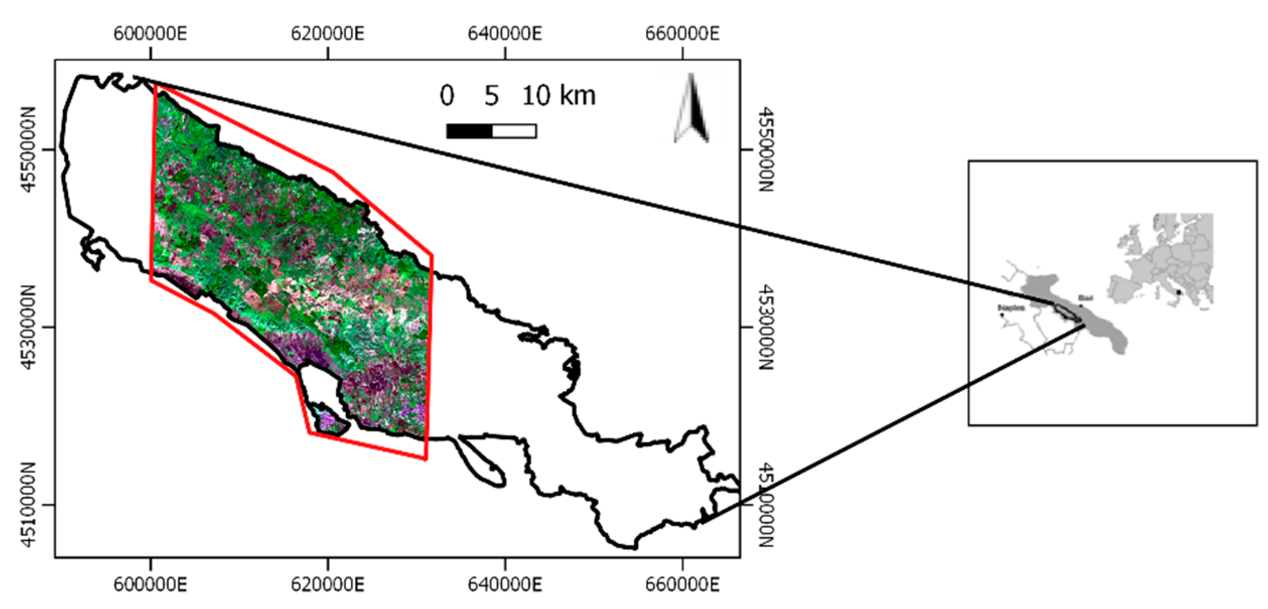
Our study area is located in the Mediterranean basin within the Apulia region, Southern Italy. The area covers nearly 800 km2 within the Natura 2000 “Murgia Alta” protected area (IT9120007) (Figure 1). This is a Site of Community Importance (SCI) and in addition a Special Protection Area (SPA) which has included a National Park since 2004.

Figure 1.
Sentinel-2 image, 10m resolution, acquired on 27 October 2018. The “Murgia Alta” protected area, the National Park and the study area in black, blue and red boundaries, respectively.
The altitude of the area is from 285 to 680 m above the sea level and its climate is mesomediterranean oceanic subcontinental pluviseasonal with dry to sub-humid ombrotype [43]. The site is characterized by a typical Mediterranean agro-pastoral landscape with millennial land-use history mainly occupied by semi-natural rocky dry grasslands, traditionally used as extensive pastures, while forest vegetation consists only of residual patches of downy oak (Quercus pubescens s.l.) woodlands and Aleppo pine (Pinus halepensis) plantations [44]. In “Murgia Alta” the same semi-natural grassland ecosystem hosts numerous regionally endemic and generally rare species, but also many with trans-Adriatic distribution [43]. This area is considered of crucial importance for the conservation of wildlife and priority species [10].
During the last three decades, this unique ecosystem has been exposed to tremendous impacts and accelerated processes of habitat degradation, fragmentation and biotic contamination (i.e., woody encroachment), both within and next to its borders. As a result of the combined pressures, ecosystems are threatened or even in danger of destruction [45]. The pressures related to degradation range from:
- the Common Agricultural Policy (CAP) which has driven the transformation of grassland pastures into agricultural (cereal crops intensification) areas by stone (rock) graining (clearance) that has induced soil erosion and sediment deposition in the aquifer system;
- the illegal waste and toxic mud dumping on transformed areas has caused heavy metal contamination of soils and aquifers;
- the increasing of traditional legal and illegal mining activities, wind farms infrastructures and arson [46,47];
- the below long-term average rainfall as a result of climate change;
- the spreading of invasive species [44,45,48].
According to the list of habitats reported in Annex I of the European Habitat Directive [9] and in EUNIS habitat taxonomies [49], the four grassland habitat types considered in “Murgia Alta” are listed in Table 1.The target habitats’ detailed description is provided in the text reported hereafter. In the text, the nomenclature of species and sintaxa follow Bartolucci et al. (2018) [50] and Biondi and Blasi (2015) [51], respectively.
2.2. Data Availability
2.2.1. Ground Truth Data
A set of reference polygons related to 9 LC classes was analyzed in the first stage of the workflow. The polygons were collected through, both, in-field campaigns and through visual interpretation of available orthophotos (2016–2018). For each class (i.e., stratum), a “stratified” sampling was adopted to ensure a minimum number of polygons–samples [53].
For ground data collection, an open source mobile application (App) was used during our in-field campaigns. This mobile App was developed within the framework of the Horizon 2020 ECOPOTENTIAL Project (www.ecopotential-project.eu). This App can gather ground truth according to Food and Agriculture Organization-Land Cover Classification System 2 (FAO-LCCS2) land cover class taxonomy [54,55,56]. By integrating additional ancillary data (e.g., lithology, soil aspects, soil surfaces), the FAO-LCCS2 taxonomy can provide a framework which may be useful to translate any LC class into different habitats [56,57,58,59,60,61,62].
For the second stage of the workflow, georeferenced surveys of the vegetation were carried out using the phytosociological method of the Sigmatista School in Zurich–Montpellier [63,64]. This method uses a floristic–statistical method based on the survey of the complete floristic composition for the plant community investigated. This approach is recognized at EU level [65,66] since it allows a precise diagnosis for many habitats of the Directive and in particular for grassland habitats. For our work, the sampling was first stratified, i.e., the relevés were carried out randomly in areas previously identified on the basis of their physiognomic and structural homogeneity. Then, all the surveys were subjected to a multivariate numerical classification by using the coverage values transformed according to the scale proposed by van der Maarel, 1979 [67]. Following this hierarchical classification, the average linkage method (UPGMA) [68] was used on the basis of the dissimilarity matrix. The latter was calculated with the reciprocal of the similarity ratio function for coverage data [64]. The clusters, thus, obtained were then attributed to the different phytosociological syntaxa on the basis of the characteristic species combination. The different plant community types, thus identified and defined, were consequently attributed to the habitats of both the EU Directive on the basis of the “Interpretation Manual of European Union habitats” [68] and the “Manuale Italiano di Interpretazione degli Habitats” [51,66,69]. Thereafter, a polygon related to a homogenous area around each relevés was identified by a visual interpretation of the available orthophoto (2018). Due to the high time-consuming process involved in the recognition and collection of the ground data, the number of reference polygons resulted to be rather small.
The data reported on Table 1 are related to four different habitat grasslands classes which correspond to the same LC class of semi-natural grasslands. In addition, a habitat map obtained by in-field campaigns and visual interpretation of a 2018 orthophoto has been recently released (2020) for the whole region by Apulia authorities.
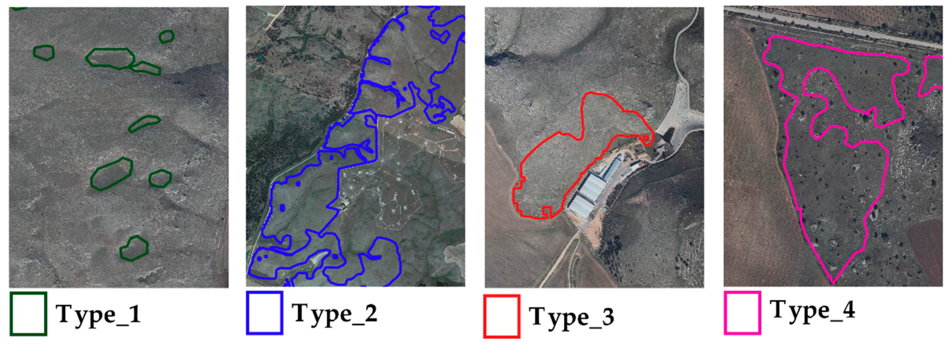
Figure 2 shows some close-ups of ground truth polygons overlaid on an orthophoto (2m spatial resolution), for the different habitat classes investigated.
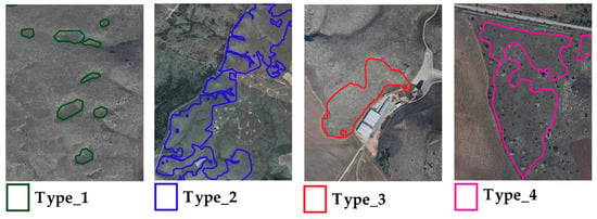
Figure 2.
Ground truth polygons overlaid on an orthophoto (2018) for different habitat classes investigated.
2.2.2. Satellite Data
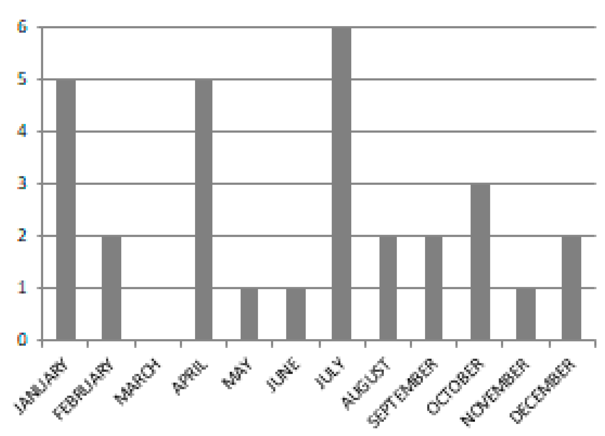
For the whole year 2018, an intra-annual time-series of Sentinel-2A/2B images was freely downloaded from the United States Geological Survey (USGS) EarthExplorer portal [70]. Only the images with less than 10% cloud cover on the full tile were investigated while the ones which showed further residual clouds in the study area were discarded. As a result, 30 clouds free images were collected, thus, no clouds/clouds shadows masking was needed. Figure 3 shows the distribution, per month, of the 30 images examined. Only in March were there no clouds free images. The dates of each image are reported in Table A1 of Appendix A.
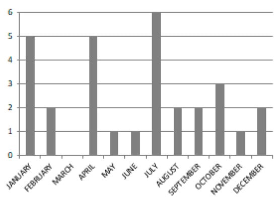
Figure 3.
Bar graph of the number of Sentinel-2 images per month.
The entire study area was covered by the tile 33TXF from the two orbits R036 and R079. Since not all images selected were available as L2A products, level-1C products were downloaded. Hence, the images in the time series to be analyzed were already geometrically orthorectified, co-registered and in at Top Of Atmosphere (TOA) reflectance. For each image, the Level-2A surface reflectance product was generated, from level-1C, by using the standalone version of the Sen2Cor processor, as suggested in [71] for atmospheric correction.
Sentinel-2 images include four spectral bands at 10 m spatial resolution in blue (B2: 458 nm–523 nm), green (B3: 543 nm–578 nm), red (B4: 650 nm–680 nm) and NIR (B8: 785 nm–899 nm) spectra. They also contain six bands at 20 m spatial resolution in red-edge (B5: 698 nm–713 nm; B6: 733 nm–748 nm; B7: 773 nm–793 nm), NIR (narrow) (B8A: 855 nm–875 nm) and Short Wave Infra-Red (SWIR) (B11: 1565 nm–1655 nm; B12: 2100 nm–2280 nm) spectra. Thus, in our work 10 spectral bands, per each image, were investigated. The three atmospheric bands (B1, B9 and B10) at 60m spatial resolution were excluded from the analysis.
To better discriminate habitats type_1 and type_4, a DTM with 8 m spatial resolution was downloaded from the Apulia Region portal [72]. The elevation information was, thus, obtained from this source.
2.2.3. Satellite Data Pre-Processing
A chain for the time-series pre-processing was implemented in the RStudio open source environment. For each image, the workflow consisted of the following steps:
- cropping according to the area of interest;
- spectral index extraction at the native spatial bands resolution;
- bilinear resampling to 10 m, when necessary. Indeed, 10 m was the final resolution adopted in our work. Different resampling approaches were tested. The bilinear one resulted the right compromise between minimization of artifacts and distortions introduced in the image as well as in the computational complexity.
Each of the spectral indices were stacked as a data-cube of intra-annual time-series in a raster file format. Table 2 shows the spectral vegetation indices analyzed singularly or in combination.

Table 2.
List of spectral indices analyzed. R stands for the Reflectance signal. The Sentinel-2 bands are reported in brackets.
The choice of these indices is based on the need to analyze the whole spectral range, from VIS to NIR, of the Sentinel-2 data. With reference to the spectral response of a vegetation pattern, we tried to take into account the information associated with the presence of a high reflectance peak in the NIR and other lower peaks in the green and SWIR. In so doing, Green Normalized Difference Vegetation Index (GNDVI) was selected to analyze the reflectance vegetation peak in the VIS spectrum region. This index is related to the photosynthetic activity and determines water and nitrogen plant uptake into the crop canopy [73,74]. As is well known, Modified Soil Adjusted Vegetation Index (MSAVI) is related to the highest peak of the vegetation reflectance in the NIR spectrum. Such an index can maximize the reduction in soil effects on the vegetation signature [74,75]. Thus, MSAVI was preferred to the widely used NDVI [48,51]. By considering Normalized Burn Ratio (NBR), the SWIR spectral information was also included. This index is correlated to water, carbon and nitrogen content as well as to vegetation health [76,77,78,79].
Further indices related to the red-edge portion of the Sentinel-2 spectrum were also introduced. The Normalized Difference Red-Edge (NDRE) [80] and Red-Edge Position (REP) [81] time-series spectral indices were extracted. All these indices were used as input to the second stage both singularly and in combinations. Only those indices providing a significant contribution to the habitat discrimination were used in combination. The results of different input configurations discussed in the present paper are reported in Table 3.

Table 3.
Different input configurations discussed in the paper.
2.3. Two-Stage Algorithm for Habitat Mapping
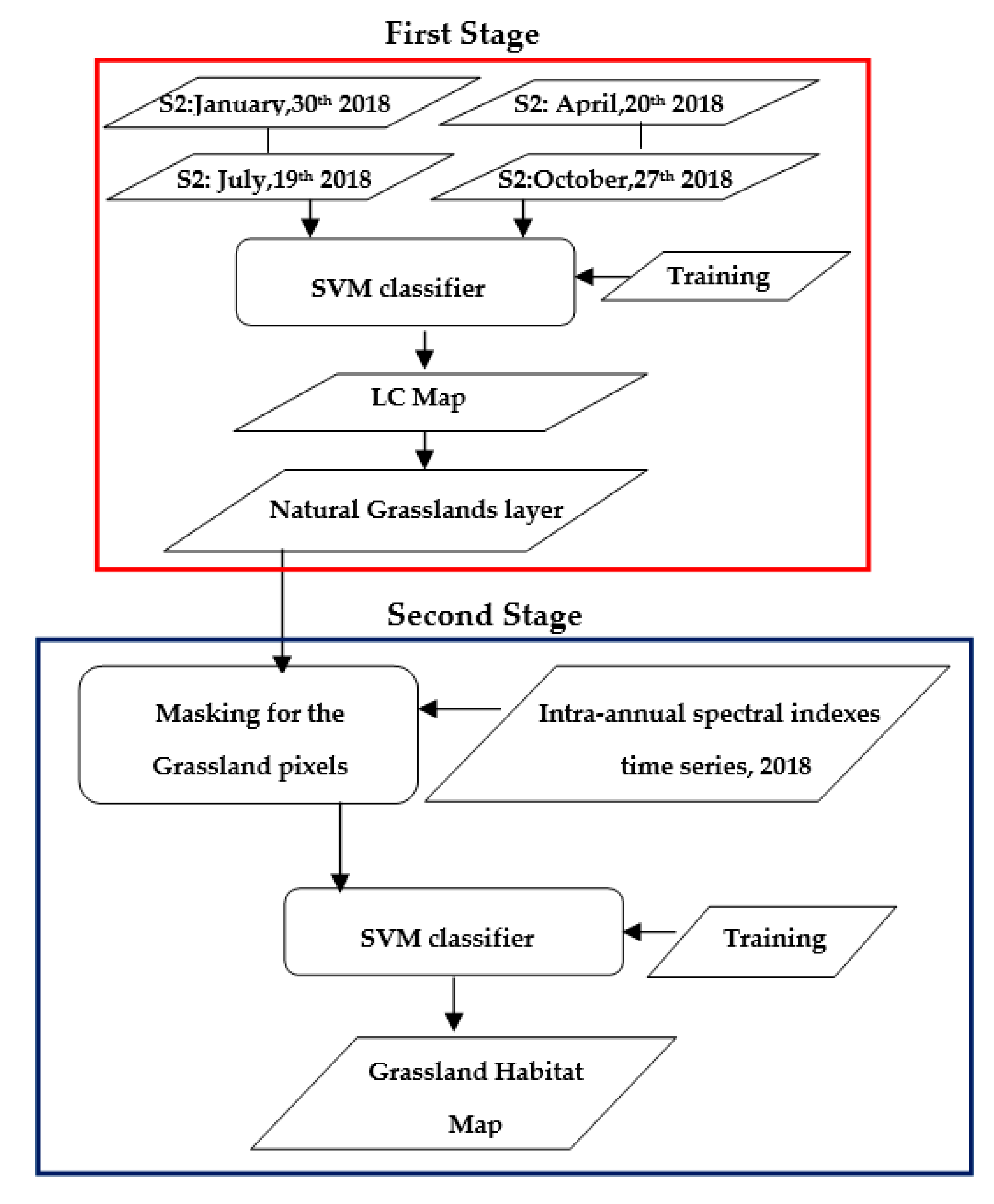
To discriminate the four grassland habitats listed in Table 1, a two-stage classification approach was developed. Figure 4 shows the two-stage algorithm workflow designed for the grassland habitats mapping. The first stage was intended to extract the grassland layer used as a pre-filter for the input features to the second stage. Two different classifiers were fed as input with a multi-season Sentinel-2 dataset. One classifier was trained for a binary (grasslands/no grasslands) classification problem and the other one for a multi-class problem. The two grassland maps obtained were compared.
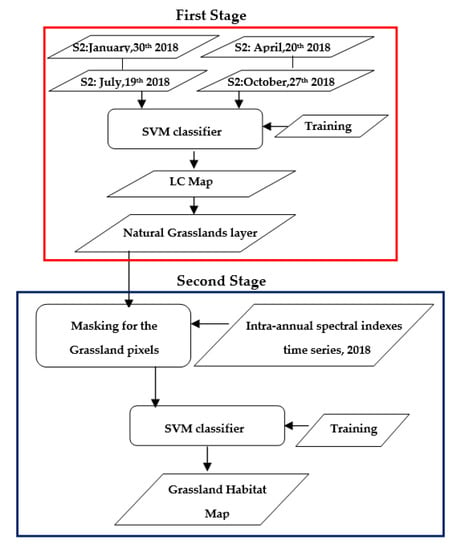
Figure 4.
Two-stage algorithm workflow for grassland habitats mapping.
The second stage focuses on the discrimination of grassland habitats. These habitats were searched within the grassland pixels recognized in the first stage LC map. For the two stages, the SVM classifier, implemented in ENVI 4.8, was used [82].
SVM is a non-linear supervised classifier aimed at finding the optimal separating hyperplane that can divide the input dataset into the predefined number of classes [83,84]. SVM classifiers are particularly well-suited when small training data sets are available with no underlying assumptions of statistical distribution [84,85,86]. Thus, SVM was adopted for our study due to the small number of training samples available. Following the recommendations reported in [87], in our study a radial basis function was selected as kernel type while the penalty parameter chosen was taken as 100. The gamma in kernel function was chosen as the inverse of the band numbers used in the data input [88,89]. Such choices were in agreement with previous research conducted by Othman and Gloaguen [90] and Yang [89].
2.3.1. First Stage
The first stage was based on a multi-class, data-driven, pixel-based, classification whose aim was to detect the grassland layer on the scene. The SVM classifier was trained with ground references from 9 LC classes, including natural grassland, labeled according to FAO-LCCS2 taxonomy [57,58,59,60,61,62]. For training the SVM classifier and subsequent validation of the output map, the available reference polygons were divided into training and validation datasets randomly per each LC class. As a result, 70% of each LC class sample was used for training and 30% for the validation, corresponding to 157,245 and 65,548 pixels, respectively. The reference polygons were distributed in the scene according to the real presence of each class on the ground. A percentage of almost 50% for natural grassland reference polygons was considered, both in the training and validation sets, since this was the dominant LC in the scene. The cultivated herbaceous vegetation was represented by almost 23% of reference polygons since this was the second major class in the scene. The remaining area was covered by both natural needle-leaved evergreen and no-herbaceous cultivated classes.
First, the classifier was fed with the input features from the stack of four multi-season images (10 bands for each image: 40 layers). Then, from the LC map obtained, the natural grassland layer was extracted to be used for the masking of the second stage input features. The pixels of the grassland layer were coded as “Natural Terrestrial Vegetation/Herbaceous”, according to LCCS2 taxonomy [62].
2.3.2. Second Stage
The second stage was employed for detecting the four different grassland habitat classes through a further data-driven, pixel-based SVM classification. Only the pixels belonging to the grassland layer found in the first stage were analyzed. For each class, the available habitat reference pixels were randomly divided into 75% and 25% to train and validate the classifier, respectively. In Table 3, the first column describes the set of input configurations adopted in the second stage. For each configuration, the second and third columns of the same table report the acronyms and the specific input features used, respectively. The output of the “4_scenes” configuration, which combines the pre-peak, peak, and post-peak of biomass with dry-season values, was compared with the ones obtained from different spectral index time-series. The latter allowed the evaluation of their inherent phenology information to improve habitat discrimination.
Since MSAVI can represent the contribution of the highest peak of the reflectance vegetation in the NIR spectrum region, the intra-annual time series of such an index was used in the first classification. For comparison purposes, GNDVI and NBR single-spectral index configurations were also analyzed. However, the findings obtained singularly are not reported in this paper since they always resulted lower than the ones from MSAVI. Nevertheless, the latter indices were successively stacked with MSAVI and used as input features to the classifier in order to enlarge the spectral coverage understudy (third and fourth configurations in Table 3). An additional configuration, which included the three spectral indices (GNDVI, MSAVI and NBR) and the DTM available, was analyzed. The fifth configuration clearly involved a computational cost related to 90 spectral layers (from the three indices) plus the DTM data used. To further reduce computational costs, the input features of the first configuration, “4_scenes”, were combined with those of only one single spectral index, i.e., MSAVI. The choice allowed the combination of the phenology (from a single-spectral index time-series) with four multi-seasonal information. The seventh configuration included the DTM layer for possible improvements related to quota information. All the analyses were carried out in a QGIS open source environment using R open source language.
2.4. Accuracy Asssessment
The protocol described in [91,92] and implemented in [93] was adopted for the classification accuracy assessment. This protocol uses the information obtained from the traditional Confusion Matrix [94] to estimate the corrected mapped area for each class and to construct confidence intervals reflecting the uncertainty of the estimates obtained.
In this framework, the sample error matrix is reported in terms of: (a) the unbiased stratified estimator of the proportion of area (pij) in each cell i,j of the matrix; (b) OA, UA and Producer’s Accuracy (PA), with standard errors estimates [91]. In addition, the F1- measure was computed as the harmonic mean of producer and user accuracies [95,96,97,98].
According to [91,92], when map categories are reported as rows (i) and the reference categories are shown as columns (j), Atot represents the total mapped area of the scene, Amapped,i is the mapped area (hectares, ha) of category i in the map and Wi = Amapped,i/Atot is the proportion of the mapped area as category i, pij is then:
where nij corresponds to sample count. The unbiased stratified estimator of the area of category j can be obtained as:
where Acorrected,j can be viewed as an “error-adjusted” estimator of area because it includes the area of omission error of category j and leaves out the area of commission error.
pij = Wi nij/ni,
Acorrected,j = Atot p.j = Atot∙∑iWi nij/ni,
The estimated standard error of the estimated proportion of area is:
S(p.j) = √(∑i = 1..qWi2((nij/ni∙)(1 − (nij/ni∙))/(ni∙ − 1)),
Finally, the standard error of the stratified area estimate can be expressed as:
and an approximate 95% confidence interval for Acorrected,j is:
S(Acorrected,j) = Atot S(p.j),
Acorrected,j ± 2S(Acorrected,j),
For each class, the measure of stratified area estimator (Acorrected) is based on the assumption that the reference validation data used for the computation of the confusion matrix can represent a proportion of the whole area [91,92].
3. Results
The investigation has been carried out to evaluate the effectiveness of an intra-annual Sentinel-2 time-series of spectral indices to improve the mapping of four Mediterranean grassland habitats in the “Murgia Alta” site. The findings, obtained from each of the configurations reported in Table 3, are presented separately below.
3.1. First Stage: Grassland Layer Extraction
In order to provide the grassland layer from the multi-seasonal input images, both a binary (grassland/no grassland) and a multi-class classification were carried out. The findings are shown in Table 4.

Table 4.
Overall Accuracy (OA)%, User’s Accuracy (UA)%, Producer’s Accuracy (PA)% values and coverage (km2) of the grassland layer obtained through binary and multi-class classification approach.
The multi-class SVM UA value was higher than the one obtained from the binary classifier: 98.29% and 96.11%, respectively. The mapping from the binary SVM classifier provided a grassland layer extension greater than the one obtained from the multi-class: 233 km2 and 223 km2, respectively. From visual interpretation of the orthophoto available, some overestimation areas appeared as misclassifications of grassland instead of crops in Figure 5.

Figure 5.
(a) Orthophoto close up on a cultivated area. Circles highlight the grassland patches. Overlaid on the orthophoto: (b) the grassland layer (yellow) from: multi-class Land Cover (LC); (c) same layer from the binary LC map.
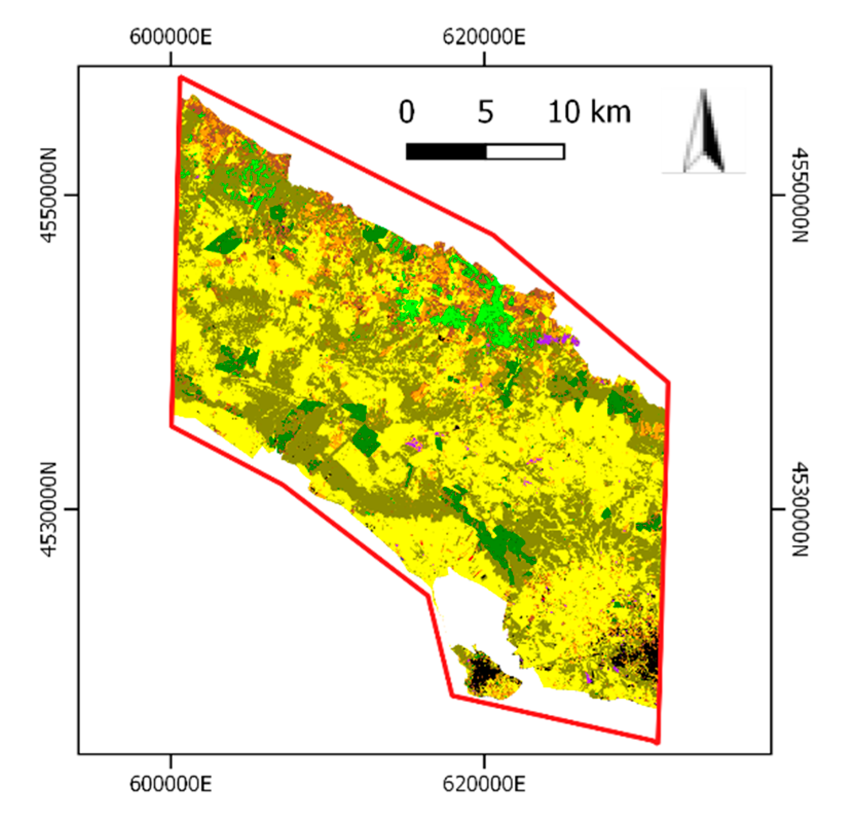
The multi-class LC map (Figure 6) was thus used to extract the grassland layer to be fed as input to the second stage.
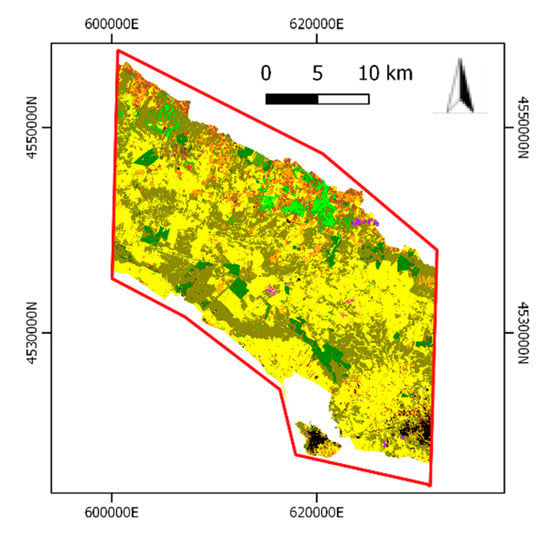
Figure 6.
First stage multi-class LC map.
Table 5 shows the nine LC classes mapped and their legend according to the FAO-LCCS2 taxonomy along with the percentage values of UA and PA. Such values can be considered quite high. Instead, misclassifications of small “Artificial Surfaces/BuiltUp” objects (i.e., sheds for depositing agriculture tools and narrow not asphalted roads) with barren land patches produced a lower UA value (61.51%).

Table 5.
LC classes legend according to FAO-LCCS2 taxonomy considered in the first stage of the workflow. UA(%) and PA(%) values are reported for each class.
The specific UA and PA values of the grassland class (Figure 7a) resulted to 98.29% ± 0.04% and 99.65% ± 0.03%, respectively.

Figure 7.
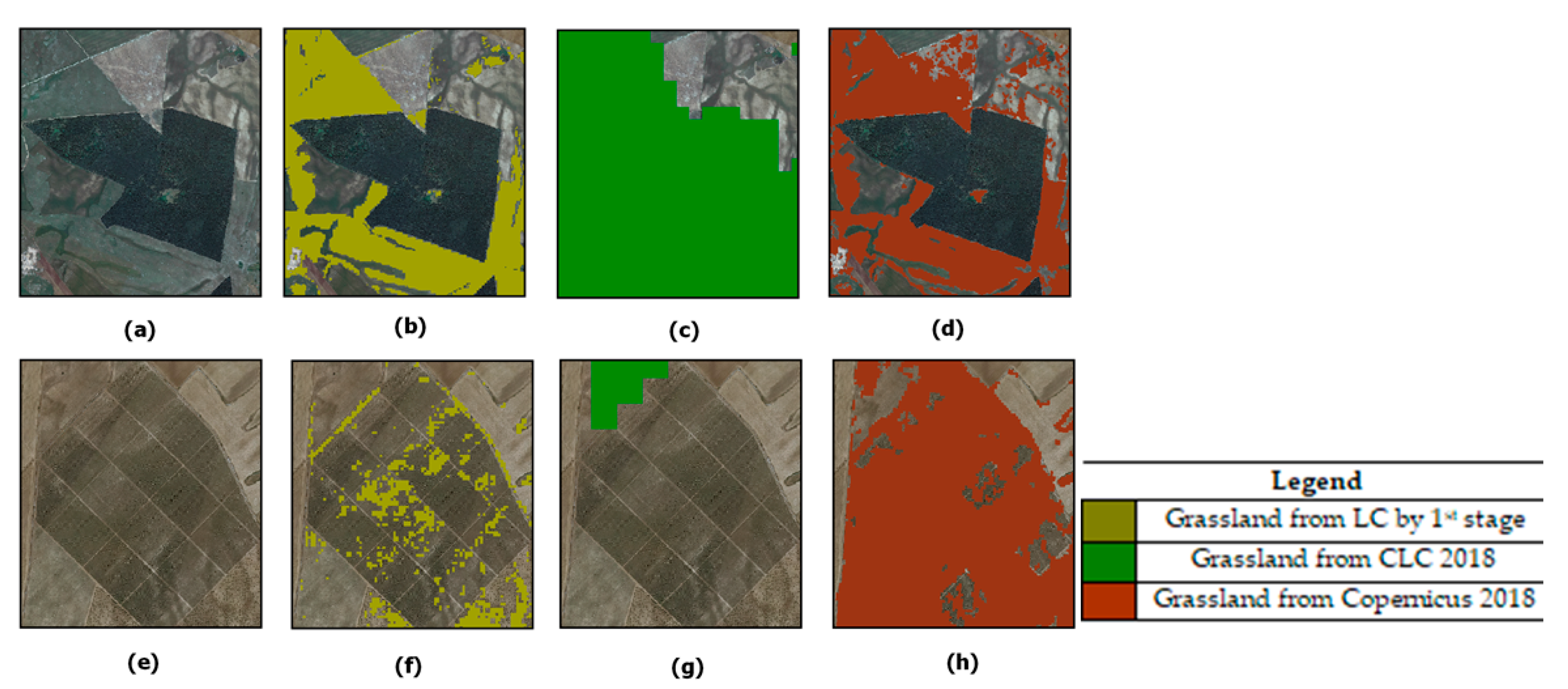
Natural grasslands layer from: (a) LC by first stage; (b) Corine Land Cover (CLC) 2018; (c) Copernicus 2018.
For comparison purpose, the grassland layer obtained from the Corine Land Cover (CLC, 100 m) map and the Copernicus High Resolution (10 m) grassland layer, both dated 2018, were analyzed and are shown in Figure 7b,c, respectively. As is well known, CLC is based on a different taxonomy (than the one used in our map, i.e., FAO-LCCS2). Thus, both 231 “Pastures” and 321 “Natural Grasslands” classes were combined to represent the CLC grassland layer. This combination resulted in a CLC layer covering 210 km2. Instead, the grassland layer from Copernicus 2018 covers an area of 250 km2. The latter product features the same resolution (10 m) as our map. The results obtained evidenced a slight overestimation by Copernicus with respect to our product (223 km2).
The accuracy of both CLC and Copernicus grassland layers was evaluated by using the same grassland validation set. The results are reported in Table 6.

Table 6.
OA%, UA%, PA% and coverage (km2) for grassland layers obtained by the first stage classifier, Corine Land Cover (CLC) and Copernicus.
Finally, the natural grassland layer, from the first stage, was used for the masking of the second stage input features.
3.2. Second Stage: Habitat Discrimination
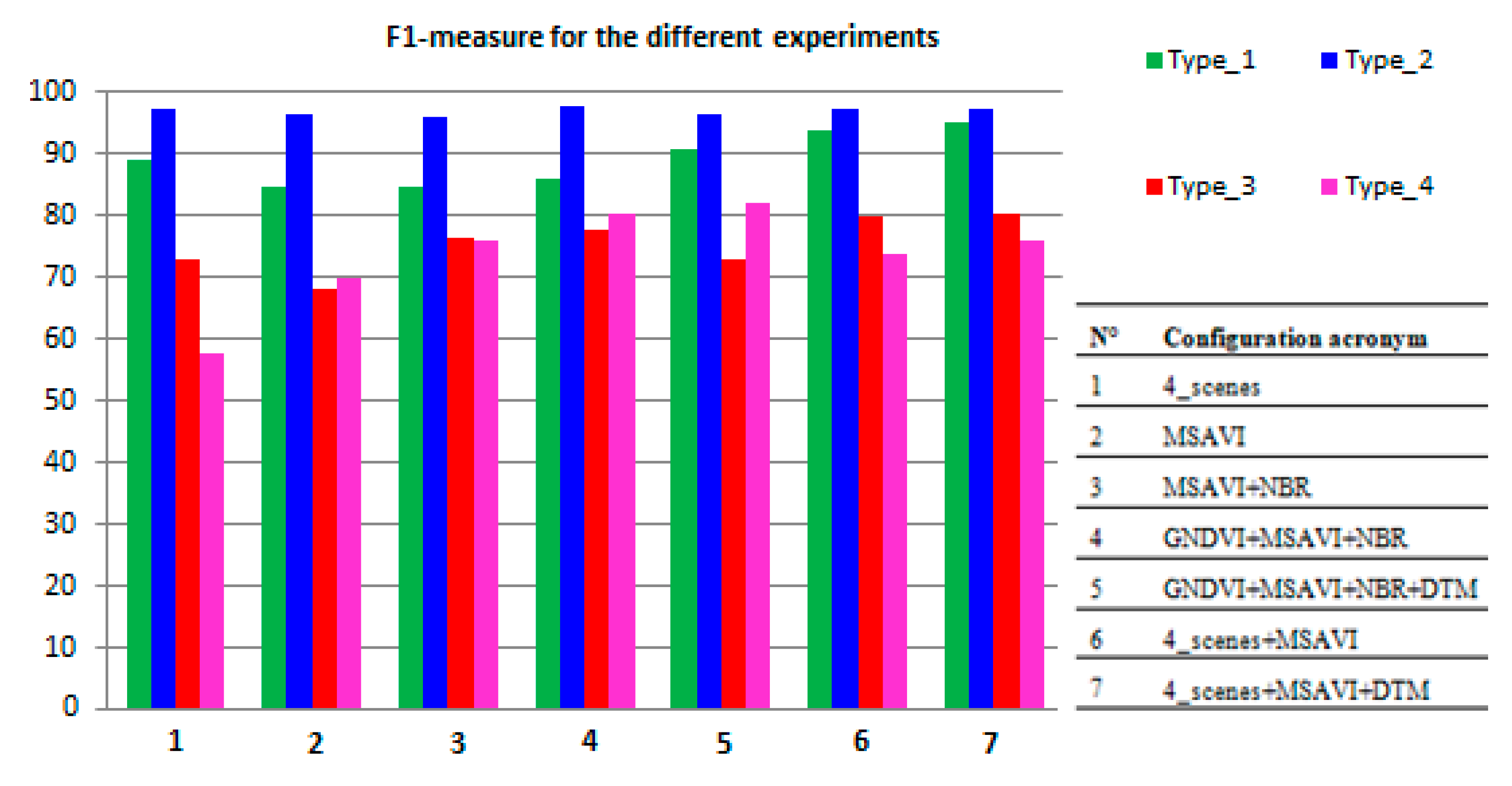
The findings obtained in terms of OA, UA, PA, F1-measure, Amapped and Acorrected are reported in Table 7 according to the different input configurations listed in Table 3. Instead, Figure 8 compares the different F1-values obtained in the form of a histogram.

Table 7.
Second stage configurations and results as UA, PA and F1 percentage values. For Areamapped vs. Areacorrected over/under-estimation in brackets.
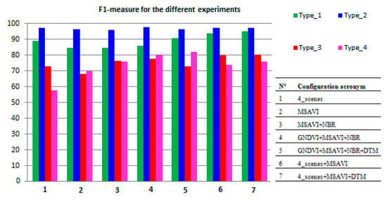
Figure 8.
Bar graph of F1-measure (%), for each habitat class, vs. different configurations.
As evidenced in Table 7, the F1-measure values obtained for type_1 and type_2 habitats resulted quite high (89.17% and 97.29%, respectively) for the “4_scenes” configuration. Instead, the F1 value for type_4 habitat resulted rather low (57.81%) due to a PA of 41.23%±0.01%. This habitat was misclassified as type_2. For the latter habitat, the Areamapped was overestimated of +646.4 ha with respect to the estimated corrected one (18875.77 ha ± 63.94 ha). Thus, discriminating type_4 would have required improvements. In fact, both PA (57.49% ± 3.76%) and F1-values (72.82%) were found to be rather low for habitat type_3. The area of this habitat resulted in an underestimation of 210.76 ha with respect to the estimated corrected value (500.66 ± 24.39). This underestimation appears to be due to misclassifications of both type_1 and type_2, thus also requiring improvements.
The configurations based on single-spectral index intra-annual time-series, i.e., “GNDVI”, “MSAVI”, “NBR”, “NDRE” and “REP” were then considered for the required improvements. These time-series provide the contribution of phenology information.
For each habitat class, better PA and UA values were obtained from “MSAVI” configuration with respect to the other ones (i.e., “GNDVI”, “NBR”, “NDRE”, “REP”). Hence, only the findings from “MSAVI” are reported in Table 7. When compared to “4_scenes”, the MSAVI intra-annual time-series provided an improvement of the F1-measure from 57.81% to 69.90% for type_4 habitat. Instead, the F1-measure resulted slightly reduced for two classes, i.e., from 89.11% to 84.60% for type_1 and from 72.82% to 68.34% for type_3. For type_2, the F1-measure remained quite stable (about 97%). This trend remained stable throughout the experiments carried out.
Pairs of spectral indices time-series were then combined to enlarge the spectrum portion analyzed. The MSAVI time-series with either GNDVI or NBR performed better than the one from single-spectral index configurations for habitats type_3 and type_4. With respect to the reference “4_scenes” results, the “MSAVI+NBR” configuration (Table 7) provided an increase in F1-measure for type_3, from 72.82% to 76.55%, and for type_4, from 57.81% to 75.88% (Table 7). This configuration performed better than “MSAVI+GNDVI”. The addition of NDRE or REP spectral indices yielded no improvement in accuracy of habitat classification, thus they were not exploited in combination with other indices.
The time-series of the three-spectral indices, “GNDVI+MSAVI+NBR”, covering the whole spectral region, were subsequently analyzed. With respect to the previous two-spectral indices configurations, slight improvements in the F1-measure were achieved for all the habitat classes. Whereas, compared to the “4_scenes” results, a significant increase in the F1-measure was achieved for habitat type_3, from 72.82% to 77.95%, and for habitat type_4, from 57.81% to 80.31%. A slight decrease was obtained, instead, for habitat type_1, from 89.11% to 86.09%.
By adding the elevation information from the DTM layer to the three “GNDVI+MSAVI+NBR” indices, some increase was achieved for habitats type_1 and type_4. With respect to the “4_scenes” configuration, a slight improvement of F1-measure was obtained for type_1 from 89.11% to 90.84%, whereas a more significant was achieved, from 57.81% to 82.21% for type_4.
Thereafter, the integration of “4_scenes” with “MSAVI” input features was tested to evaluate the advantage of combining dense temporal information, from an intra-annual single-index time-series, with the spectral bands of the four multi-season images. By reducing the input dimensionality from 90 (30 images per each of the three indices) to 70 (10 bands per each of the four images, plus 30 MSAVI values), the computation complexity decreased. With respect to the “4_scenes” configuration, the F1-measure improved from 89.11% to 93.73%, from 72.82% to 79.97% and from 57.81% to 73.95%, respectively, for three habitats, i.e., type_1, type_3 and type_4. Whereas, the F1 value remained stable for class type_2.
Finally, the DTM layer was added to the previous configuration (“4_scenes + MSAVI”). The OA value obtained remained almost the same (95.45% ± 0.30%), whereas the F1-measure was the highest among the whole set of configurations for type_1 and type_3, as reported in Table 7. Compared to the “4_scenes” results, the F1 values improved from 89.11% to 95.25%, from 72.82% to 80.27% and from 57.81% to 75.97%, respectively, for type_1, type_3 and type_4. However, the F1 value remained stable for class type_2 (Table 7).
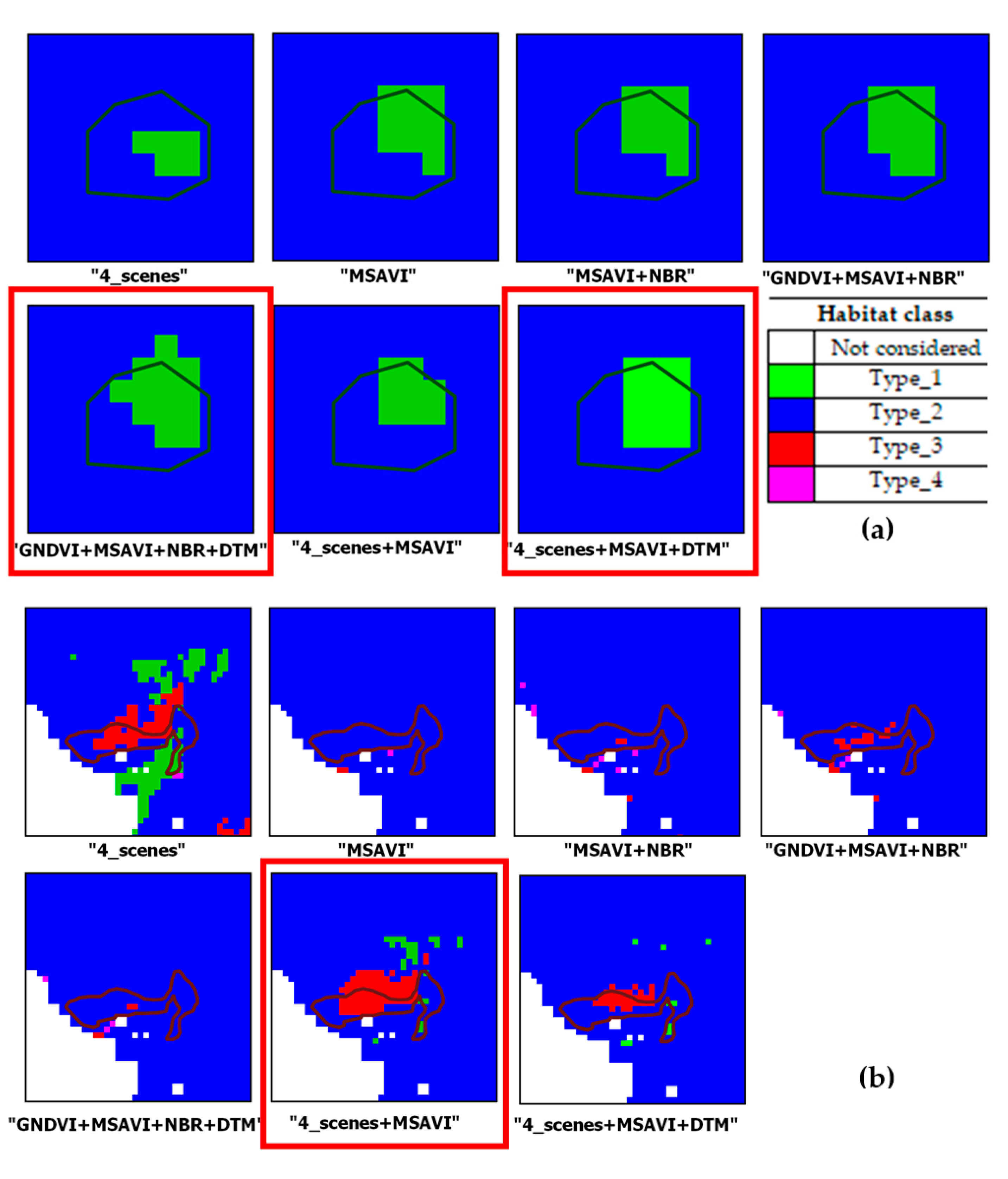
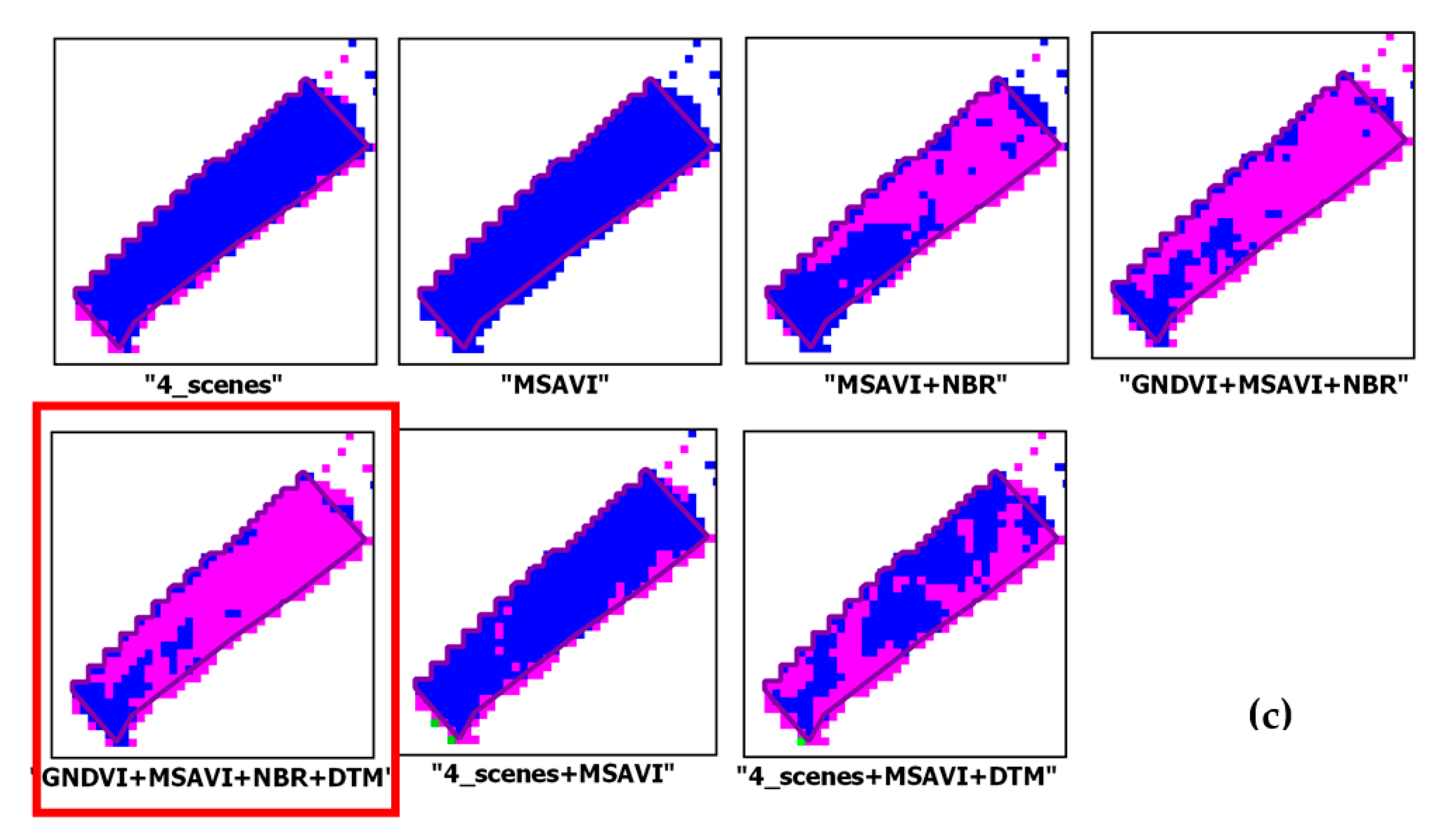
Figure 9 shows some close-ups of the output maps obtained from the seven configurations analyzed for habitats type_1, type_3 and type_4.
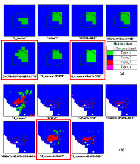

Figure 9.
Close-ups from output maps from the input configurations analyzed. Each habitat reference polygon overlaid on the maps. A red frame highlights the best result. Patches for habitat class: (a) Type_1; (b) Type_3; (c) Type_4.
Figure 9 shows examples of output grassland habitats varying with the input features of the classifier. For habitat type_1, the addition of the DTM to both “GNDVI+MSAVI+NBR” and “4_scenes + MSAVI” improved the recognition of the patch (Figure 9a). For habitat type_3, the best result appeared the one from “4_scenes + MSAVI” (Figure 9b). For habitat type_4 (Figure 9c) the best discrimination occurred with “GNDVI+MSAVI+NBR+DTM”.
In order to provide quantitative evaluations of the whole scene classification, the corrected stratified area estimator (per each class) and its standard error within 95% confidence interval values are also reported in Table 7. The values found allowed quantification of habitat over/under-estimations over the whole area mapped. Several problems of over/underestimation are evidenced in this Table. For type_1 habitat, the Areamapped was overestimated with respect to the Areacorrected in all the configurations (“plus” sign in brackets, Table 7). The Areamapped reported the lowest value (1418.27 ha) when “MSAVI” configuration was analyzed, while the highest value (2481.36 ha) was obtained from “4_scenes + MSAVI”configuration.
Habitat type_2 is the dominant class in the scene and thus the most represented in the training samples. For this habitat, the highest Areamapped and overestimation values (19,808.83 ha and + 608.10 ha) were obtained from the “MSAVI”, whereas the lowest values (18,092.50 ha and + 467.83) were achieved from the “GNDVI + MSAVI + NBR + DTM” configuration.
Habitats type_3 and type_4 were underestimated in all the configurations (“minus” sign in brackets, Table 7). These habitats were misclassified not only with the dominant class type_2 but also with the type_1. For type_3 the highest Areamapped value (429.30 ha) was obtained from “MSAVI+NBR” while the lowest (289.90 ha) value was achieved from “4_scenes”. For type_4 the highest (1751.57 ha) and the lowest (449.57 ha) Areamapped values resulted from “GNDVI + MSAVI + NBR + DTM” and “4_scenes” configurations, respectively. For all the configurations explored, the findings reported required an improvement to reduce the over/underestimations described. For this purpose, a combination of the classifiers outputs was carried out through a majority vote (MV) technique [99].
Combination of Different Configurations
For each pixel, the MV algorithm can read the label obtained from the seven configurations and then may assign the pixel analyzed to the most frequent class found. In the present study, we chose as the most frequent class the label assigned by at least four classifiers out of seven. The OA obtained was 95.72% ± 0.29%. The criteria of the most frequent class were unsatisfactory for only 0.9% of the pixels classified. To each pixel an uncertainty value was assigned. This value was defined as the number of classifiers in disagreement with the final MV output class.
Table 8 reports the OA obtained by the validation pixels which can satisfy each uncertainty value. As can be noted, to a decrease in the uncertainty corresponds an increase in the OA value. As a result, the overestimation of habitat type_1 was reduced. For each class, Table 9 compares the habitat coverage obtained by MV with the one from the best single configuration found, i.e., “4_scenes + MSAVI + DTM”.

Table 8.
Majority vote results with uncertainty and OA values.

Table 9.
Habitat coverage obtained from majority vote (MV) compared with “4_scenes+MSAVI+DTM” configuration.
Figure 10 and Figure 11 report some close-ups which evidence the reduction in habitat type_1 overestimation through the MV. Specifically, Figure 10 shows the reduction in type_1 pixels performed by the MV. As can be noted, the MV confirms type_1 patches classified by more than four classifiers but cleans up the remaining type_1 pixels in favor of habitat type_2. The MV impact is also evident in Figure 11. In this figure, pixels misclassified as type_4 by the “4_scenes+MSAVI+DTM” configuration were mostly correctly assigned as type_2 (Figure 11b). The related uncertainty values are shown in Figure 11c.
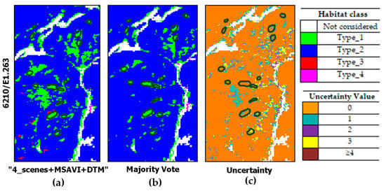
Figure 10.
Close-ups from classified maps obtained by: (a) the best classifier configuration (“4_scenes + MSAVI + DTM”); (b) the MV. Uncertainty map in (c) with dark polygons evidencing reference habitat type_1 patches on the ground.
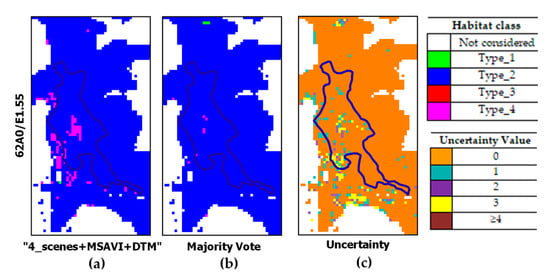
Figure 11.
Close-ups from classified maps obtained by: (a) the best classifier configuration (“4_scenes + MSAVI + DTM”); (b) the MV; (c) uncertainty map with blue polygons evidencing reference habitat type_2 patches on the ground.
Figure 12 reports an example of a habitat type_4 patch. For this patch, the classifier, “4_scenes+MSAVI+DTM” provides a better habitat classification than MV. The latter classifier increased the pixels belonging to type_2 habitat.
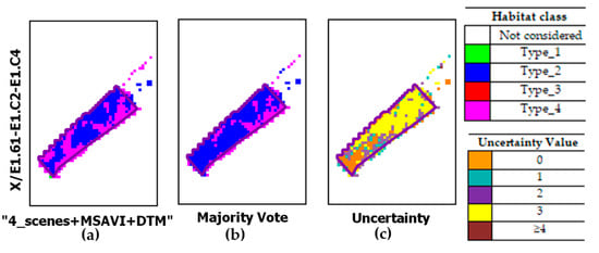
Figure 12.
Close-ups from classified maps obtained by: (a) the classifier configuration (“4_scenes + MSAVI + DTM”); (b) the MV; (c) uncertainty map. Dark polygons show the reference type_4 habitat patch on the ground.
The MV behavior found in the last case evidenced the failure to solve misclassifications associated to a specific class, as also evidenced in [100,101]. In our study, the failure concerning habitat type_4 may be due to several issues: first, a non-adequate reference training collection; second, the semantic habitat description adopted for habitat discrimination. Thus, these issues may have influenced the performance of all classifiers.
4. Discussion
The present work aimed at mapping four semi-natural dry grassland habitats in the “Murgia Alta” Natura 2000 site (i.e., 6210/E1.263, 62A0/E1.55, 6220/E1.434 and X/E1.61-E1.C2-E1.C4 as described in Table 1) by means of Sentinel-2 data intra-annual time-series. A time-series of only 30 clouds-free images was used over a total number of 132 images regularly acquired in 2018 by Sentinel-2.
In previous papers, the grassland layer was obtained by ancillary data which were not always either updated or available at the same spatial scale [13,32,35,36]. Thus, in such studies, the grassland layer accuracies reported could have affected the quality of the habitat mapping. In this paper, instead, the first stage of the classification system was employed to provide a grassland layer and a habitat map obtained at the same date.
In the first stage of the proposed system, a binary (grassland/non-grassland) and a multi-class approach were first tested and compared for the extraction of the grassland layer. The findings revealed slight differences between the two approaches with higher accuracy and lower misclassifications obtained by the multi-class classifier. Specifically, the multi-class classification produced a grassland layer with high OA, UA and PA of 98.94%, 98.31% and 99.60%, respectively. This layer was extracted from the same images used for habitat mapping in the second stage.
The grassland layer can also be extracted from a CLC map. An additional opportunity is offered by the recent availability of the Copernicus grassland service. However, these grassland products are not yearly updated. The CLC inventory was initiated in 1985 (reference year 1990). Updates have been produced in 2000, 2006, 2012, and 2018. Available Copernicus grassland layers are dated 2015 and 2018.
To evaluate the available grassland services, the layer obtained from our first stage was thus compared with the grassland layer extracted by the existing CLC map and the high resolution Copernicus grassland one (10 m), both available for 2018. The quantitative comparison results (Table 6) have evidenced that the best grasslands OA was achieved by the SVM (98.94 ± 0.08) classifier of our first stage system with four multi-season images as input. A qualitative analysis of specific areas in the three outputs compared can evidence some important misclassifications found in both the CLC and the Copernicus layers. For example, Figure 13a shows a woodland patch surrounded by grasslands in an orthophoto. Figure 13b–d show the grasslands pixels as obtained by the three products compared: our first stage output, the CLC and the Copernicus grasslands layers, respectively. As can be observed, both our first stage classifier (Figure 13b) and the Copernicus service (Figure 13d) do correctly identify the grasslands pixels, whereas the CLC (Figure 13c) overestimated such pixels also covering the woodland area.
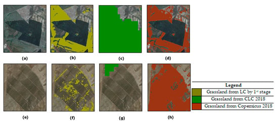
Figure 13.
(a) Close-up of a wood patch from an orthophoto; (b) grasslands pixels from our first stage overlaid to the orthophoto; (c) CLC grasslands pixels; (d) Copernicus grasslands pixels; (e) a crop area in the orthophoto; (f) grasslands pixels from our first stage overlaid to the orthophoto; (g) CLC grasslands pixels; (h) Copernicus grasslands pixels (in red).
An additional example is provided in Figure 13e–h. Specifically, Figure 13e shows an agricultural area in the orthophoto. As can be noted in Figure 13f, our first stage classifier misclassified only a few (natural) grasslands pixels (label A12/A2 in Table 5) in the cultivated area. Figure 13g shows correctly, that the CLC did not detect any grassland pixels in the same area. This is due to the inclusion of land use information in CLC map as well as to its lower resolution with respect to our product (10 m). Figure 13h, instead, evidences a misclassification of grasslands in the Copernicus layer (20 m). Such a result is due to the fact that the Copernicus service can provide only LC information.
For the first-stage output of the system, the findings have confirmed both the usefulness of high resolution (10 m) data and the multi-class analysis adopted, with respect to the binary approach. Thus, the proposed first-stage setting has adequately extracted the grassland layer to be used in the second stage for habitat mapping. In addition, this layer can be updated whenever a new habitat map is required, at the same spatial and temporal image resolution.
For the second stage of the system, the introduction of times-series of spectral indices improved habitat discrimination. The results obtained were better than the ones by analyzing only the four multi-season data sets (first configuration, Table 7) including the biomass pre-peak (30 January), peak (20 April), post-peak (27 October) and the dry season (19 July) for grasslands. The hypothesis justifying these findings can be the fact that plant communities composing the habitats under study may not contemporarily reach these phases, as also reported by Rapinel et al. (2019). For example, the therophytic communities, including type_3 and part of type_4, are composed by different species with different times of biomass peak. Some of them can reach the peak in April, others toward the end of May (Table 1).
By adding the MSAVI time series to the “4_scenes” configuration, we intensified phenology information. The choice to add MSAVI time series was due to the better results achieved with respect to GNDVI and NBR, evaluated singularly (Section 3.2). In addition, MSAVI can represent the contribution of the reflectance vegetation highest peak in the NIR spectrum region.
Following the suggestion by Groβe-Stoltenbeg et al. [37], a three-indice time series (i.e., GNDVI+MSAVI+NBR) covering the whole Sentinel-2 spectral range from VIS to NIR, was analyzed. The results achieved were quite comparable in terms of F1 measurements with the ones obtained from our “4_scenes+MSAVI” configuration. The OA value reported from these two configurations (93.97% and 95.29%, respectively) were better than the one (91%) obtained by Schuster et al. (2015) [1]. These authors extracted three spectral indices (NDVI, NDVI-RE-R, NDVI-NIR-RE) from a one-year Rapid-Eye time-series obtained spanning over three vegetation periods from April 2009 to September 2011 to achieve a rather dense and relatively homogenous intra-annual time series. However, the spectral indices chosen by these authors and the satellite data used were different from ours.
As evidenced by Favel et al. (2019), DTM can yield management information useful for the discrimination of habitats characterized by similar phenology and spectral features. In particular, in our study area, lower quotas are more accessible for pastures. Thus, they are subjected to sheep grazing. Such living stock feeding can advantage or inhibit the presence of plant species, which characterize specific habitats. Thus, when DTM information was added to configurations selected a further improvement was achieved for OA values and in particular for F1 findings (Table 7). Specifically, F1 values for classes type_1 and type_3 obtained from “4_scenes + MSAVI + DTM” (70 input layers) were 95.25% and 80.27%, respectively. These values were better than the ones resulting from “GNDVI + MSAVI + NBR + DTM” (90 input layers), i.e., 90.84% and 73.02%, respectively. These results may be due to the well-known over-fitting phenomena which occurs when the dimension of input configuration is rather high with respect to the small size of the available training set [101].
With respect to habitat type_1, our results are in agreement with the ones obtained by Marcinkowska-Ochtyra (2019) through the integration of DTM with hyperspectral data. In terms of UA and PA, our findings (86.09% and 96.15%), are better than the ones reported by Zlinszky et al. (2014) (66.4% and 78.6%), obtained by using Lidar data from two different campaigns.
For each input pixel, the “4_scenes + MSAVI + DTM” configuration involved 71 values, i.e., 10 bands for each of the four images analyzed, plus 30 MSAVI values from the time series and the specific pixel elevation value. Instead, the “GNDVI+MSAVI+NBR+DTM”, involved 91 values, i.e., three index values per 30 images and elevation. Thus, the former configuration resulted in a reduction in computational costs. This reduction did not require the application of a pre-processing phase for feature extraction as done by Rapinel et al. (2019). These authors analyzed the phenology information embedded in the whole set of spectral bands of a Sentinel-2 time-series (12 images) instead of spectral indices. By reducing the input bands from 120 to 26, they mapped seven grassland plant communities, thus reporting an OA of 78%. This result is lower than the one obtained from both our “GNDVI + MSAVI + NBR + DTM” and “4_scenes + MSAVI + DTM” configurations (Table 7).
Thus, phenology information from Sentinel-2 time series can better discriminate grassland habitats with different times of increase and decrease speed of photosynthesis, start/end of growing season, duration of photosynthetic activity [102,103]. Such metrics, which are generally collected through in-field campaigns, appear embedded in the time series indices.
This finding suggests that neither four multi-season images nor phenology information extracted from a single spectral index alone may be sufficient to discriminate the grassland habitats under study. Instead, the combined use of phenology and spectral bands of four multi-season images (last configuration) can guarantee the achievement of rather high F1-measures values for most of the habitat classes considered (Table 7). The highest F1-measures accuracies could be obtained for type_1 and type_3 (95.25% and 80.27%, respectively) whereas the accuracy for type_2, that was already very high with the first “4_scenes” configuration (F1-measure equal to 97.29%), remained stable in all the experiments. For type_4 habitat the F1-measure was the lowest (75,97%) of the configurations analyzed. This might be due to the fact that species reach Biomass Peak in the first half of April, occasionally in late March. However, no cloud free images were available in March (Table A1, Appendix A) to extract MSAVI spectral index values in that month. Moreover, only two images were available from the first half of April (8 and 13 April). Actually, a rather denser intra-annual spectral index time-series would have helped in discriminating this habitat from the others in the Biomass Peak period. To this aim, gap filling techniques of clouded images should be applied in future work [78,104].
The application of the MV reduced the misclassifications of type_1. Thus, a slight improvement of the OA (up to 2%) with respect to the OA of each specific configuration was obtained by combining the outputs of all the configurations. These findings, together with the difficulty of identifying the optimal classifier for all four of the habitats, make the MV approach attractive for mapping. Equally evidenced by Foody et al., (2007) [105], although not yielding the most accurate classification, the MV can provide useful information on classification uncertainties. These values can be used for post-classification fieldwork aimed to collect additional training/validation reference samples and reduce in-field costs in future campaigns.
Figure 14 shows a close-up of a woodland area where an attempt at reforestation must have failed. Overlaid on the orthophoto, the following maps are shown: Figure 14a, the regional map evidencing type_2 pixels located only in the surrounding woodland area; Figure 14b, the “GNDVI + MSAVI + NBR + DTM” map showing both type_2 and type_4 habitat pixels within the woody patch; Figure 14c, “4_scenes + MSAVI + DTM” map reporting, within the woody patch, type_2 pixels, but showing less type_4 pixels than in Figure 14b; Figure 14d, the MV map based on the convergence of ≥4 classifiers; such a map appears similar to the one in Figure 14c; Figure 14e, the uncertainty map of the area evidencing higher values for pixels assigned to type_4 habitat.
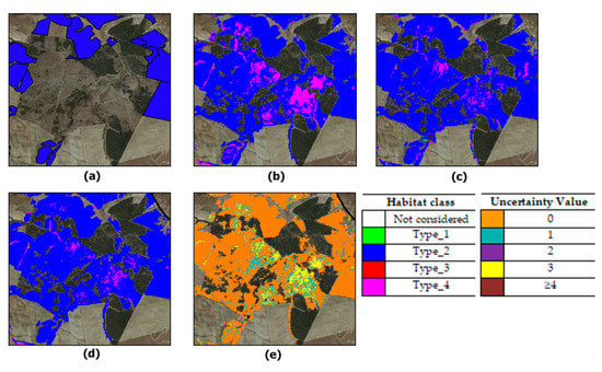
Figure 14.
The 2018 orthophoto close ups: (a) habitat map available, from Apulia Regional portal (2020); (b–d) output maps from “GNDVI + MSAVI + NBR + DTM”, “4_scenes + MSAVI + DTM” and Majority Vote, respectively; (e) uncertainty map.
Besides the quantitative results reported above, the qualitative comparison carried out in Figure 14 evidences that the automatic two-stage mapping proposed in our study can recognize the presence of type_2 and type_4 in the area analyzed. In this area, in-field campaigns had not been carried out by the local expert involved in the regional mapping. In fact, to reduce in-field campaigns costs, the expert ecologists generally use visual interpretation of available orthophotos. However, such orthophotos generally cover only single season information. Thus, the approach proposed in our work can provide updated habitat maps and related uncertainty values on a large scale. In turn, these values may represent a valuable support for specific in-field investigations.
5. Conclusions
The aim of the present study was to investigate the improvements that can be obtained by exploiting phenology information extracted from intra-annual indices time-series of Sentinel-2 data for mapping grassland habitats in “Murgia Alta”. Based on multi-seasonal information from four Sentinel-2 images, the first classification stage provided an updated grassland layer. At the local scale, this layer showed less misclassified pixels than the ones from CLC and Copernicus services. In the second stage, the combination of four multi-seasonal spectral band images with both the phenology embedded in the MSAVI spectral index time-series and DTM, provided more reliable habitats discrimination. Nevertheless, the Majority Vote ensemble of the different second-stage input configurations used offered uncertainty measures useful for addressing in-field campaigns for validation purposes. In a future study, to improve the discrimination of the habitats, gap filling techniques will be implemented for obtaining more dense time-series.
The habitat mapping of a Natura 2000 sites must be updated every 6 years, according to the European Habitat Directive. For large areas, this task may be achieved by developing cost/time-efficient automatic tools such as the ones proposed in the present study. The two-stage classification system proposed, which is based on the use of machine learning algorithms, could contribute to speeding up the design of both urgent conservation policies and sustainable regeneration actions of natural ecosystems. This would address both the drastic biodiversity loss and the ongoing climatic changes.
The availability of habitat maps updated both at high temporal and spatial resolutions is very important for decision making at local levels. Therefore, updated habitats maps could be useful variables for monitoring the achievement of Sustainable Development Goal 15 (SDG 15) aimed towards halting biodiversity loss (https://sdgs.un.org/goals/goal15).
Author Contributions
Conceptualization, P.B., C.T., M.A.; methodology, C.T., M.A., P.B.; software, C.T., S.V.; validation, C.T., L.F., V.T.; formal analysis, P.B., C.T., M.A.; investigation, C.T., M.A.; resources, C.T., L.F., M.A., S.V., V.T.; data curation, C.T., L.F., M.A., S.V., V.T.; writing—original draft preparation, C.T.; writing—review and editing, C.T., M.A., L.F., V.T., C.B, P.B.; visualization, C.T.; supervision, P.B., C.T., L.F., C.B., V.T., M.A.; project administration, P.B.; funding acquisition, P.B. All authors have read and agreed to the published version of the manuscript.
Funding
This research was funded by the H2020 E-SHAPE project—EuroGEO Showcases: Applications Powered by Europe (www.e-shape.eu), Grant Agreement: 820852 and by the COHECO project—Sistema Integrato di Monitoraggio, Allerta e Prevenzione dello stato di COnservazione di Habitat ed ECOsistemi in aree interne e costiere protette e da proteggere (www.coheco.it) in the framework of the POR Puglia FESR-FSE 2014–2020.
Institutional Review Board Statement
Not applicable.
Informed Consent Statement
Not applicable.
Data Availability Statement
Data sharing not yet available.
Acknowledgments
The authors are grateful to “Murgia Alta” National Park Authority for the remarkable ecological support and to Maria Tarantino for the patient reviewing of the English version of the paper.
Conflicts of Interest
The authors declare no conflict of interest. The funders had no role in the design of the study; in the collection, analyses, or interpretation of data; in the writing of the manuscript, or in the decision to publish the results.
Appendix A

Table A1.
Date of acquisition for the 30 images in the time-series. The symbol ° indicates those dates used in the first stage. Double lines point out each month.
Table A1.
Date of acquisition for the 30 images in the time-series. The symbol ° indicates those dates used in the first stage. Double lines point out each month.
| Acquisition Date | Sensor |
|---|---|
| 2018-01-03 | S2A |
| 2018-01-05 | S2B |
| 2018-01-18 | S2B |
| 2018-01-25 | S2B |
| 2018-01-30° | S2A |
| 2018-02-12 | S2A |
| 2018-02-14 | S2B |
| No cloud free images in March | |
| 2018-04-08 | S2B |
| 2018-04-13 | S2A |
| 2018-04-20° | S2A |
| 2018-04-23 | S2A |
| 2018-04-30 | S2A |
| 2018-05-25 | S2B |
| 2018-06-12 | S2A |
| 2018-07-02 | S2A |
| 2018-07-09 | S2A |
| 2018-07-12 | S2A |
| 2018-07-14 | S2B |
| 2018-07-19° | S2A |
| 2018-07-22 | S2A |
| 2018-08-01 | S2A |
| 2018-08-28 | S2A |
| 2018-09-12 | S2B |
| 2018-09-22 | S2B |
| 2018-10-20 | S2A |
| 2018-10-25 | S2B |
| 2018-10-27° | S2A |
| 2018-11-09 | S2A |
| 2018-12-04 | S2B |
| 2018-12-09 | S2A |
References
- Schuster, C.; Schmidt, T.; Conrad, C.; Kleinschmit, B.; Forster, M. Grassland habitat mapping by intra-annual time-series analysis-Comparison of RapidEye and TerraSAR-X satellite data. Int. J. Appl. Earth Obs. GeoInf. 2015, 34, 25–34. [Google Scholar] [CrossRef]
- Hector, A.; Schmid, B.; Beierkuhnlein, C.; Caldeira, M.C.; Diemer, M.; Dimitrakopoulos, P.G.; Finn, J.A.; Freitas, H.; Giller, P.S.; Good, J.; et al. Plant diversity and productivity of European grasslands. Science 1999, 286, 1123–1127. [Google Scholar] [CrossRef] [PubMed]
- Fraser, L.H.; Pither, J.; Jentsch, A.; Sternberg, M.; Zobel, M.; Askarizadeh, D.; Bartha, S.; Beierkuhnlein, C.; Bennett, J.; Bittel, A.; et al. Worldwide evidence of a unimodal relationship between productivity and plant species richness. Science 2015, 349, 302–305. [Google Scholar] [CrossRef] [PubMed]
- Dengler, J.; Janišová, M.; Török, P.; Wellstein, C. Biodiversity of Palaearctic grasslands: A synthesis. Agric. Ecosyst. Environ. 2014, 182, 1–14. [Google Scholar] [CrossRef]
- O’Mara, F. The role of grasslands in food security and climate change. Ann. Bot. 2012, 110, 1263–1270. [Google Scholar] [CrossRef] [PubMed]
- Habel, J.C.; Dengler, J.; Janišová, M.; Török, P.; Wellstein, C.; Wiezik, M. European grassland ecosystems: Threatened hotspots of biodiversity. Biodivers. Conserv. 2013, 22, 2131–2138. [Google Scholar] [CrossRef]
- Newbold, T.; Hudson, L.N.; Arnell, A.P.; Contu, S.; De Palma, A.; Ferrier, S.; Hill, S.L.L.; Hoskins, A.J.; Lysenko, I.; Phillips, H.R.P.; et al. Has land use pushed terrestrial biodiversity beyond the planetary boundary? A global assessment. Science 2016, 353, 288–291. [Google Scholar] [CrossRef]
- Wellstein, C.; Poschlod, P.; Gohlke, A.; Chelli, S.; Campetella, G.; Rosbakh, S.; Canullo, R.; Kreyling, J.; Jentsch, A.; Beierkuhnlein, C. Effects of extreme drought on specific leaf area of grassland species: A meta-analysis of experimental studies in temperate and sub-Mediterranean systems. Glob. Chang. Biol. 2017, 23, 2473–2481. [Google Scholar] [CrossRef]
- Council Directive 92/43/EEC. Available online: https://eur-lex.europa.eu/legal-content/EN/TXT/?uri=celex%3A31992L0043 (accessed on 1 July 2013).
- Council Directive 2009/147/EEC. Available online: https://eur-lex.europa.eu/legal-content/EN/TXT/?uri=CELEX%3A32009L0147 (accessed on 26 June 2019).
- CBD. Available online: https://www.cbd.int/convention/articles/?a=cbd-01 (accessed on 11 February 2006).
- Natura 2000, EU. Available online: https://ec.europa.eu/environment/nature/natura2000/index_en.htm (accessed on 11 November 2008).
- Buck, O.; Garcia Millàn, V.E.; Klink, A.; Pakzad, K. Using information layers for mapping grassland habitat distribution at local to regional scales. Int. J. Appl. Earth Obs. Geoinf. 2015, 37, 83–89. [Google Scholar] [CrossRef]
- Mehner, H.; Cutler, M.; Fairbairn, D.; Thompson, G. Remote sensing of upland vegetation: The potential of high spatial resolution satellite sensors. Glob. Ecol. Biogeogr. 2004, 13, 359–369. [Google Scholar] [CrossRef]
- Hill, M.J.; Ticehurst, C.J.; Lee, J.; Fellow, L.; Grunes, M.R.; Donald, G.E.; Henry, D. Integration of optical and radar classifications for mapping pasture type in Western Australia. IEEE Trans. Geosci. Remote Sens. 2005, 43, 1665–1681. [Google Scholar] [CrossRef]
- Schmidtlein, S.; Zimmermann, P.; Schüpferling, R.; Weiß, C. Mapping the floristic continuum: Ordination space position estimated from imaging spectroscopy. J. Veg. Sci. 2007, 18, 131–140. [Google Scholar] [CrossRef]
- Schuster, C.; Ali, I.; Lohmann, P.; Frick, A.; Förster, M.; Kleinschmit, B. Towards detecting swath events in TerraSAR-X time-series to establish Natura 2000 grassland habitat swath management as monitoring parameter. Remote Sens. 2011, 3, 1308–1322. [Google Scholar] [CrossRef]
- Wright, C.K.; Wimberly, M.C. Recent land use change in the Western Corn Belt threatens grasslands and wetlands. Proc. Natl. Acad. Sci. USA 2013. [Google Scholar] [CrossRef] [PubMed]
- Feilhauer, H.; Thonfeld, F.; Faude, U.; He, K.S.; Rocchini, D.; Schmidtlein, S. Assessing floristic composition with multispectral sensors—A comparison based on monotemporal and multiseasonal field spectra. Int. J. Appl. Earth Observ. Geoinf. 2013, 21, 218–229. [Google Scholar] [CrossRef]
- Nagendra, H.; Lucas, R.M.; Honrado, J.P.; Jongman, R.; Tarantino, C.; Adamo, P.; Mairota, P. Remote sensing for conservation monitoring: Assessing protected areas, habitat extent, habitat condition, species diversity and threats. Ecol. Indic. 2013, 33, 45–59. [Google Scholar] [CrossRef]
- Turner, W.; Spector, S.; Gardiner, N.; Fladeland, M.; Sterling, E.; Steininger, M. Remote sensing for biodiversity science and conservation. Trends Ecol. Evol. 2003, 18, 306–314. [Google Scholar] [CrossRef]
- Strand, H.; Höft, R.; Strittholt, J.; Horning, N.; Miles, L.; Fosnight, E.; Turner, W. Sourcebook on Remote Sensing and Biodiversity Indicators; Technical Series; Secretariat of the Convention on Biological Diversity: Montreal, QC, Canada, 2007. [Google Scholar]
- Wang, K.; Franklin, S.E.; Guo, X.; Cattet, M. Remote sensing of ecology, bio-diversity and conservation: A review from the perspective of remote sensing specialists. Sensors 2010, 10, 9647–9667. [Google Scholar] [CrossRef]
- Franke, J.; Keuck, V.; Siegert, F. Assessment of grassland use intensity by remote sensing to support conservation schemes. J. Nat. Conserv. 2012, 20, 125–134. [Google Scholar] [CrossRef]
- Corbane, C.; Alleaume, S.; Deshayes, M. Mapping natural habitats using remote sensing and sparse partial least square discriminant analysis. Int. J. Remote Sens. 2013, 34, 7625–7647. [Google Scholar] [CrossRef]
- Zlinszky, A.; Schroiff, A.; Kania, A.; Deák, B.; Mücke, W.; Vári, A.; Székely, B.; Pfeifer, N. Categorizing Grassland Vegetation with Full-Waveform Airborne Laser Scanning: A Feasibility Study for Detecting Natura 2000 Habitat Types. Remote Sens. 2014, 6, 8056–8087. [Google Scholar] [CrossRef]
- Landmann, T.; Piiroinen, R.; Makori, D.M.; Abdel-Rahman, E.M.; Makau, S.; Pellikka, P.; Raina, S.K. Application of hyperspectral remote sensing for flower mapping in African savannas. Remote Sens. Environ. 2015, 166, 50–60. [Google Scholar] [CrossRef]
- Möckel, T.; Dalmayne, J.; Schmid, B.C.; Prentice, H.C.; Hall, K. Airborne hyperspectral data predict fine-scale plant species diversity in grazed dry grasslands. Remote Sens. 2016, 8, 133. [Google Scholar] [CrossRef]
- Gholizadeh, H.; Gamon, J.A.; Townsend, P.A.; Zygielbaum, A.I.; Helzer, C.J.; Hmimina, G.Y.; Yu, R.; Moore, R.M.; Schweiger, A.K.; Cavender-Bares, J. Detecting prairie biodiversity with airborne remote sensing. Remote Sens. Environ. 2019, 221, 38–49. [Google Scholar] [CrossRef]
- Oldeland, J.; Wesuls, D.; Rocchini, D.; Schmidt, M.; Jürgens, N. Does using species abundance data improve estimates of species diversity from remotely sensed spectral heterogeneity? Ecol. Indic. 2010, 10, 390–396. [Google Scholar] [CrossRef]
- Marcinkowska-Ochtyra, A.; Gryguc, K.; Ochtyra, A.; Kopeć, D.; Jarocinska, A.; Sławik, L. Multitemporal Hyperspectral Data Fusion with Topographic Indices—Improving Classification of Natura 2000 Grassland Habitats. Remote Sens. 2019, 11, 2264. [Google Scholar] [CrossRef]
- Wen, Q.; Zhang, Z.; Liu, S.; Wang, X.; Wang, C. Classification of grassland types by MODIS time-series images in Tibet, China. IEEE J. Sel. Top. Appl. Earth Obs. Rem. Sens. 2010, 3, 3. [Google Scholar] [CrossRef]
- Copernicus ESA Program. Available online: https://www.esa.int/Applications/Observing_the_Earth/Copernicus (accessed on 22 June 2018).
- Drusch, M.; Bello, U.D.; Carlier, S.; Colin, O.; Fernandez, V.; Gascon, F.; Hoersch, B.; Isola, C.; Laberinti, P.; Martimort, P.; et al. Sentinel-2: ESA’s optical high-resolution mission for GMES operational services. Remote Sens. Environ. 2012, 120, 25–36. [Google Scholar] [CrossRef]
- Fauvel, M.; Lopes, M.; Dubo, T.; Rivers-Moore, J.; Frison, P.; Gross, N.; Ouin, A. Prediction of plant diversity in grasslands using Sentinel-1 and -2 satellite image time-series. Remote Sens. Environ. 2020, 237, 111536. [Google Scholar] [CrossRef]
- Rapinel, S.; Mony, C.; Lecoq, L.; Clément, B.; Thomas, A.; Hubert-Moy, L. Evaluation of Sentinel-2 time-series for mapping floodplain grassland plant communities. Remote Sens. Environ. 2019, 223, 115–129. [Google Scholar] [CrossRef]
- Groβe-Stoltenbeg, A.; Hellmann, C.; Werner, C.; Oldeland, J.; Thiele, J. Evaluation of continuous VNIR-SWIR pectra versus narrowband hyperspectral indices to discriminate the invasive Acacia longifolia within a Mediterranean dune ecosystem. Remote Sens. 2016, 8, 334. [Google Scholar] [CrossRef]
- Vapnik, V.N. The Nature of Statistical Learning Theory; Springer: New York, NY, USA, 1995. [Google Scholar]
- Vapnik, V.N. Statistical Learning Theory; Wiley: New York, NY, USA, 1998. [Google Scholar]
- Rabe, A.; van der Linden, S.; Hostert, P. Simplifying Support Vector Machines for classification of hyperspectral imagery and selection of relevant features. In Proceedings of the 2nd Workshop of Hyperspectral Image and Signal Processing: Evolution in Remote Sensing (WHISPERS), Reykjavik, Iceland, 14–16 June 2010. [Google Scholar] [CrossRef]
- Grabska, E.; Frantz, D.; Ostapowicz, K. Evaluation of machine learning algorithms for forest stand species mapping using Sentinel-2 imagery and environmental data in the Polish Carpathians. Remote Sens. Environ. 2020, 251, 112103. [Google Scholar] [CrossRef]
- Maxwell, A.E.; Warner, T.A.; Fang, F. Implementation of machine-learning classification in remote sensing: An applied review. Int. J. Remote Sens. 2018, 39, 2784–2817. [Google Scholar] [CrossRef]
- Forte, L.; Perrino, E.V.; Terzi, M. Le praterie a Stipa austroitalica Martinovsky ssp. austroitalica dell’Alta Murgia (Puglia) e della Murgia Materana (Basilicata). Fitosociologia 2005, 42, 83–103. [Google Scholar]
- Mairota, P.; Leronni, V.; Xi, W.; Mladenoff, D.; Nagendra, H. Using spatial simulations of habitat modification for adaptive management of protected areas: Mediterranean grassland modification by woody plant encroachment. Environ. Conserv. 2013, 41, 144–146. [Google Scholar] [CrossRef]
- Mairota, P.; Cafarelli, B.; Labadessa, R.; Lovergine, F.; Tarantino, C.; Lucas, R.M.; Nagendra, H.; Didham, R.K. Very high resolution Earth observation features for monitoring plant and animal community structure across multiple spatial scales in protected areas. Int. J. Appl. Earth Obs. Geoinf. 2015, 37, 100–105. [Google Scholar] [CrossRef]
- Sutter, G.C.; Brigham, R.M. Avifaunal and habitat changes resulting from conversion of native prairie tocrested wheat grass: Patterns at songbird community and species levels. Can. J. Zool. 1998, 76, 869–875. [Google Scholar] [CrossRef]
- Brotons, L.; Pons, P.; Herrando, S. Colonization of dynamic Mediterranean landscapes: Where do birds come from after fire? J. Biogeogr. 2005, 32, 789–798. [Google Scholar] [CrossRef]
- Tarantino, C.; Casella, F.; Adamo, M.; Lucas, R.; Beierkuhnlein, C.; Blonda, P. Ailanthus altissima mapping from multi-temporal very high resolution satellite images. ISPRS J. Photogram. Remote Sens. 2019, 147, 90–103. [Google Scholar] [CrossRef]
- Davies, C.E.; Moss, D. EUNIS Habitat Classification. In Final Report to the European Topic Centre of Nature Protection and Biodiversity; European Environment Agency: Swindon, UK, 2002. [Google Scholar]
- Bartolucci, F.; Peruzzi, L.; Galasso, G.; Albano, A.; Alessandrini, A.; Ardenghi, N.M.G.; Astuti, G.; Bacchetta, G.; Ballelli, S.; Banfi, E.; et al. An updated checklist of the vascular flora native to Italy. Plant Biosyst. 2018, 152, 179–303. [Google Scholar] [CrossRef]
- Biondi, E.; Blasi, C. Prodromo della Vegetazione Italiana 2015. Ministero dell’Ambiente e della Tutela del Territorio e del Mare. Available online: http://www.prodromo-vegetazione-italia.org/ (accessed on 1 March 2015).
- Perrino, E.V.; Brunetti, G.; Farrag, K. Plant Communities in Multi-Metal Contaminated Soils: A Case Study in the National Park of Alta Murgia (Apulia Region—Southern Italy). Int. J. Phytoremediat. 2014, 16, 871–888. [Google Scholar] [CrossRef]
- Congalton, R.G.; Gu, J.; Yadav, K.; Thenkabail, P.; Ozdogan, M. Global Land Cover Mapping: A Review and Uncertainty Analysis. Remote Sens. 2014, 6, 12070–12093. [Google Scholar] [CrossRef]
- Di Gregorio, A.; Jansen, L.J.M. Land Cover Classification System (LCCS): Classification Concepts and User Manual; Food and Agriculture Organization of the United Nations: Rome, Italy, 2005. [Google Scholar]
- Lucas, R.; Tomaselli, V.; Mitchell, A. Deliverable 4.2 (EO Biophysical Parameters, Land Use and Habitats Extraction Modules) of the Horizon2020 Project “ECOPOTENTIAL: Improving Future Ecosystem Benefits through Earth Observations” (G.A. 641762). Available online: http://www.ECOPOTENTIAL-project.eu (accessed on 5 March 2020).
- Masò, J.; Domingo-Marimon, C.; Lucas, R. Deliverable 10.3 of the Horizon2020 Project “ECOPOTENTIAL: Improving Future Ecosystem Benefits through Earth Observations” (G.A. 641762). Implementation of Apps. Research Report. 2018. Available online: http://www.ECOPOTENTIAL-project.eu (accessed on 5 March 2020).
- Tomaselli, V.; Dimopoulos, P.; Marangi, C.; Kallimanis, A.S.; Adamo, M.; Tarantino, C.; Panitsa, M.; Terzi, M.; Veronico, G.; Lovergine, F.; et al. Translating land cover/land use classifications to habitat taxonomies for landscape monitoring: A Mediterranean assessment. Landsc. Ecol. 2013, 28, 905–930. [Google Scholar] [CrossRef]
- Adamo, M.; Tarantino, C.; Tomaselli, V.; Kosmidou, V.; Petrou, Z.; Manakos, I.; Lucas, R.M.; Mücher, C.A.; Veronico, G.; Marangi, C.; et al. Expert knowledge for translating land cover/use maps to general habitat categories (GHC). Landsc. Ecol. 2014, 29, 1045–1067. [Google Scholar] [CrossRef]
- Lucas, R.M.; Blonda, P.; Bunting, P.F.; Jones, G.; Inglada, J.; Arias, M.; Kosmidou, V.; Petrou, Z.; Manakos, I.; Adamo, M.; et al. The Earth observation data for habitat monitoring (EODHaM) system. Int. J. Appl. Earth Obs. Geoinf. 2015, 37, 17–28. [Google Scholar] [CrossRef]
- Adamo, M.; Tarantino, C.; Tomaselli, V.; Veronico, G.; Nagendra, H.; Blonda, P. Habitat mapping of coastal wetlands using expert knowledge and Earth observation data. J. Appl. Ecol. 2016, 53, 1521–1532. [Google Scholar] [CrossRef]
- Gavish, Y.; O’Connel, J.; Marsh, C.J.; Tarantino, C.; Blonda, P.; Tomaselli, V.; Kunin, W.E. Comparing the performance of flat and hierarchical Habitat/Land-Cover classification models in a NATURA 2000 site. ISPRS J. Photogram. Remote Sens. 2018, 136, 1–12. [Google Scholar] [CrossRef]
- Adamo, M.; Tomaselli, V.; Tarantino, C.; Vicario, S.; Veronico, G.; Lucas, R.; Blonda, P. Knowledge-based classification of grassland ecosystem based on multi-temporal WorldView-2 data and FAO-LCCS taxonomy. Remote Sens. 2020, 12, 1447. [Google Scholar] [CrossRef]
- Braun-Blanquet, J. Pflanzensoziologie: Grundzüge der Vegetationskunde; Plant Sociology Basics of Vegetation Science; Springer: Berlin/Heidelberg, Germany, 1964; pp. 287–399. [Google Scholar]
- Westhoff, V.; van der Maarel, E. The Braun-Blanquet Approach. In Classification of Plant Communities; Whittaker, R.H., Ed.; Junk: The Hague, The Netherlands, 1978; pp. 287–399. [Google Scholar]
- EU. Habitats Manual, Interpretation Manual of European Union habitats: 1–144. 2013. Available online: http://ec.europa.eu/environment/nature/legislation/habitatsdirective/docs/Int_Manual_EU28.pdf (accessed on 1 April 2013).
- Biondi, E.; Blasi, C.; Burrascano, S.; Casavecchia, S.; Copiz, R.; Del Vico, E.; Galdenzi, D.; Gigante, D.; Lasen, C.; Spampinato, G.; et al. Manuale Italiano di Interpretazione Degli Habitat della Direttiva 92/43/CEE. MATTM-DPN, SBI. 2010. Available online: http://vnr.unipg.it/habitat/index.jsp (accessed on 1 December 2007).
- Van der Maarel, E. Transformation of cover-abundance values in phytosociology and its effects on community similarity. Vegetation 1979, 39, 97–114. [Google Scholar]
- Sokal, R.R.; Michener, C.D. A Statistical Method for Evaluating Systematic Relationships. Univ. Kansas Sci. Bull. 1958, 38, 1409–1438. [Google Scholar]
- Biondi, E.; Burrascano, S.; Casavecchia, S.; Copiz, R.; Del Vico, E.; Galdenzi, D.; Gigante, D.; Lasen, C.; Spampinato, G.; Venanzoni, R.; et al. Diagnosis and syntaxonomic interpretation of Annex I Habitats (Dir. 92/43/ EEC) in Italy at the alliance level. Plant Sociol. 2012, 49, 5–37. [Google Scholar]
- USGS Portal. Available online: https://earthexplorer.usgs.gov/ (accessed on 9 May 2018).
- ESA Technical Guide. Available online: https://sentinel.esa.int/web/sentinel/technical-guides/sentinel-2-msi/level-2a-processing (accessed on 26 March 2018).
- Puglia Region Portal. Available online: www.sit.puglia.it (accessed on 1 February 2014).
- Gitelson, A.; Kaufman, Y.; Merzlyak, M.N. Use of green channel in remote sensing of global vegetation from EOS-MODIS. Remote Sens. Environ. 1996, 58, 289–298. [Google Scholar] [CrossRef]
- Barati, S.; Rayegani, B.; Saati, M.; Sharifi, A.; Nasri, M. Comparison the accuracies of different spectral indices for estimation of vegetation cover fraction in sparse vegetated areas. Egypt. J. Remote Sens. Space Sci. 2011, 14, 49–56. [Google Scholar] [CrossRef]
- Qi, J.; Chehbouni, A.; Huete, A.R.; Kerr, Y.H. Modified Soil Adjusted Vegetation Index (MSAVI). Remote Sens. Environ. 1994, 48, 119–126. [Google Scholar] [CrossRef]
- Lopez-Garcia, M.; Caselles, V. Mapping burns and natural reforestation using Thematic Mapper data. Geocarto Int. 1991, 6, 31–37. [Google Scholar] [CrossRef]
- Lutes, D.C.; Keane, R.E.; Caratti, J.F.; Key, C.H.; Benson, N.C.; Sutherland, S.; Gangi, L.J. General Technical Report RMRS-GTR-164-CD; FIREMON: Fire Effects Monitoring and Inventory System, Ed.; Department of Agriculture, Forest Service, Rocky Mountains Research Station: Fort Collins, CO, USA, 2006. [CrossRef]
- Vicario, S.; Adamo, M.; Alcaraz-Segura, D.; Tarantino, C. Bayesian Harmonic Modelling of Sparse and Irregular Satellite Remote Sensing Time-series of Vegetation Indexes: A Story of Clouds and Fires. Remote Sens. 2020, 12, 83. [Google Scholar] [CrossRef]
- Asner, G.P.; David, B. Lobell. A Biogeophysical Approach for Automated SWIR Unmixing of Soils and Vegetation. Remote Sens. Environ. 2000, 74.1, 99–112. [Google Scholar] [CrossRef]
- Zhang, K.; Ge, X.; Shen, P.; Li, W.; Liu, X.; Cao, Q.; Zhu, Y.; Cao, W.; Tian, Y. Predicting Rice Grain Yield Based on Dynamic Changes in Vegetation Indexes during Early to Mid-Growth Stages. Remote Sens. 2019, 11, 387. [Google Scholar] [CrossRef]
- Main, R.; Cho, M.A.; Mathieu, R.; O’Kennedy, M.M.; Ramoelo, A.; Koch, S. An investigation into robust spectral indices for leaf chlorophyll estimation. ISPRS J. Photogramm. Remote Sens. 2011, 66, 751–761. [Google Scholar] [CrossRef]
- Harris Geospatial Solutions. Available online: www.harris.com/solution/envi (accessed on 5 March 2015).
- Huang, C.; Davis, L.S.; Townshend, J.R.G. An assessment of support vector machines for land cover classification. Int. J. Remote Sens. 2002, 23, 725–749. [Google Scholar] [CrossRef]
- Mountrakis, G.; Im, J.; Ogole, C. Support vector machines in remote sensing: A review. ISPRS J. Photogramm. Remote Sens. 2011, 66, 247–259. [Google Scholar] [CrossRef]
- Foody, G.M.; Mathur, A. A relative evaluation of multiclass image classification by support vector machines. IEEE Trans. Geosci. Remote Sens. 2004, 6, 1335–1343. [Google Scholar] [CrossRef]
- Waske, B.; Van der Linden, S. Classifying multilevel imagery from SAR and optical sensors by decision fusion. IEEE Trans. Geosci. Remote Sens. 2008, 46, 1457–1466. [Google Scholar] [CrossRef]
- Othman, A.A.; Al-Maamar, A.F.; Al-Manmi, D.A.; Liesenberg, V.; Hasan, S.E.; Obaid, A.K.; Al-Quraishi, A.M. GIS-based modeling for selection of Dam sites in the Kurdistan region, Iraq. Int. J. Geo-Inf. 2020, 9, 244. [Google Scholar] [CrossRef]
- Othman, A.A.; Gloaguen, R. Improving lithological mapping by SVM classification of spectral and morphological features: The discovery of a new chromite body in the Mawat ophiolite complex (Kurdistan, NE Iraq). Remote Sens. 2014, 6, 6867–6896. [Google Scholar] [CrossRef]
- Yang, X. Parameterizing support vector machines for land cover classification. Photogramm. Eng. Remote Sens. 2011, 77, 27–38. [Google Scholar] [CrossRef]
- Othman, A.; Al-Saady, Y.; Al-Khafaji, A.; Gloaguen, R. Environmental change detection in the central part of Iraq using remote sensing data and GIS. Arab. J. Geosci. 2014, 7, 1017–1028. [Google Scholar] [CrossRef]
- Olofsson, P.; Foody, G.M.; Stehman, S.V.; Woodcock, C.E. Making better use of accuracy data in land change studies: Estimating accuracy and area and quantifying uncertainty using stratified estimation. Remote Sens. Environ. 2013, 129, 122–131. [Google Scholar] [CrossRef]
- Olofsson, P.; Foody, G.M.; Herold, M.; Stehman, S.V.; Woodcock, C.E.; Wulder, M.A. Good practices for estimating area and assessing accuracy of land change. Remote Sens. Environ. 2014, 148, 42–57. [Google Scholar] [CrossRef]
- Tarantino, C.; Adamo, M.; Lucas, R.; Blonda, P. Detection of changes in semi-natural grasslands by cross correlation analysis with WorldView-2 images and new Landsat 8 data. Remote Sens. Environ. 2016, 175, 65–72. [Google Scholar] [CrossRef]
- Congalton, R.G.; Kass, G. Assessing the Accuracy of Remotely Sensed Data: Principle and Practices, 2nd ed.; Taylor & Francis Group: Abingdon, UK, 2009; ISBN 9781420055122. [Google Scholar]
- Sasaki, Y. The Truth of the F-Measure; 2007. Available online: https://www.toyota-ti.ac.jp/Lab/Denshi/COIN/people/yutaka.sasaki/F-measure-YS-26Oct07.pdf (accessed on 26 October 2007).
- Halder, A.; Ghosh, A.; Ghosh, S. Aggregation pheromone density based pattern classification. Fundam. Inform. 2009, 92, 345–362. [Google Scholar]
- Schuster, C.; Förster, M.; Kleinschmit, B. Testing the red edge channel for improving land-use classifications based on high-resolution multi-spectral satellite data. Int. J. Remote Sens. 2012, 33, 5583–5599. [Google Scholar] [CrossRef]
- Baumann, M.; Ozdogan, M.; Kuemmerle, T.; Wendland, K.J.; Esipova, E.; Radeloff, V.C. Using the Landsat record to detect forest-cover changes during and after the collapse of the Soviet Union in the temperate zone of European Russia. Remote Sens. Environ. 2012, 124, 174–184. [Google Scholar] [CrossRef]
- Tulyakov, S.; Jaeger, S.; Govindaraju, V.; Doermann, D. Review of classifier combination methods. Mach. Learn. Doc. Anal. Recognit. 2008, 90, 361–386. [Google Scholar]
- Xiaoshuang, M.; Huanfeng, S.; Jie, Y.; Liangpei, Z.; Pingxiang, L. Polarimetric-Spatial Classification of SAR Images Based on the Fusion of Multiple Classifiers. IEEE J. Sel. Top. Appl. Earth Obs. Remote Sens. 2014, 7, 961–971. [Google Scholar] [CrossRef]
- Xue, Y. An overview of Overfitting and its solutions. J. Phys. Conf. Ser. 2019. [Google Scholar] [CrossRef]
- Clerici, N.; Weissteiner, C.J.; Halabuk, A.; Hazeu, G.; Roerink, G.; Mücher, S. Phenology Related Measures and Indicators at Varying Spatial Scales; Alterra Report; 2012; p. 2259. ISSN 1566-7197. Available online: https://edepot.wur.nl/199907 (accessed on 1 January 2012).
- Jönsson, P.; Cai, Z.; Melaas, E.; Friedl, M.A.; Eklundh, L. A Method for Robust Estimation of Vegetation Seasonality from Landsat and Sentinel-2 Time Series Data. Remote Sens. 2018, 10, 635. [Google Scholar] [CrossRef]
- Griffiths, P.; Nendel, C.; Hostert, P. Intra-annual reflectance composites from Sentinel-2 and Landsat for national-scale crop and land cover mapping. Remote Sens. Environ. 2019, 220, 135–151. [Google Scholar] [CrossRef]
- Foody, G.M.; Boyd, D.S.; Sanchez-Hernandez, C. Mapping a specific class with an ensemble of classifiers. Int. J. Remote Sens. 2007, 28, 1733–1746. [Google Scholar] [CrossRef]
Publisher’s Note: MDPI stays neutral with regard to jurisdictional claims in published maps and institutional affiliations. |
© 2021 by the authors. Licensee MDPI, Basel, Switzerland. This article is an open access article distributed under the terms and conditions of the Creative Commons Attribution (CC BY) license (http://creativecommons.org/licenses/by/4.0/).

