Abstract
Given the high financial and institutional cost of collecting and processing accurate topography data, many large-scale flood hazard assessments continue to rely instead on freely-available global Digital Elevation Models, despite the significant vertical biases known to affect them. To predict (and thereby reduce) these biases, we apply a fully-convolutional neural network (FCN), a form of artificial neural network originally developed for image segmentation which is capable of learning from multi-variate spatial patterns at different scales. We assess its potential by training such a model on a wide variety of remote-sensed input data (primarily multi-spectral imagery), using high-resolution, LiDAR-derived Digital Terrain Models published by the New Zealand government as the reference topography data. In parallel, two more widely used machine learning models are also trained, in order to provide benchmarks against which the novel FCN may be assessed. We find that the FCN outperforms the other models (reducing root mean square error in the testing dataset by 71%), likely due to its ability to learn from spatial patterns at multiple scales, rather than only a pixel-by-pixel basis. Significantly for flood hazard modelling applications, corrections were found to be especially effective along rivers and their floodplains. However, our results also suggest that models are likely to be biased towards the land cover and relief conditions most prevalent in their training data, with further work required to assess the importance of limiting training data inputs to those most representative of the intended application area(s).
1. Introduction
The most recent Global Assessment Report on Disaster Risk Reduction [1] highlights that low- and middle-income countries continue to be disproportionately impacted by natural hazards, in terms of both fatalities and economic losses relative to GDP. While there are many complex and inter-connected reasons for this [2], the research presented here addresses one in particular–data scarcity. Understanding the spatial and temporal variation in the intensity of a given hazard, as well as the potential impacts on communities and economic assets exposed to it, requires access to high-resolution and reliable data. Disaster risk assessments in lower-income countries often face significant constraints in this regard, given the high financial costs and long-term institutional capacity necessary for collecting, processing and storing high-quality datasets describing the relevant hazards [1].
We focus on flood hazards in particular, which accounted for almost a quarter of all disaster-related economic losses over the past decade [3] and continue to pose a significant threat to life, particularly in low- and middle-income countries [1]. Looking ahead, these negative impacts are likely to worsen due to rising sea levels and the increasing hydro-meteorological variability associated with climate change [4], as well as increasing exposure related to fast-growing cities in low-income countries, most of which are located along the coast or a major river [2].
For any quantitative assessment of likely flood hazards (and related phenomena, such as tsunami inundation and the effects of sea level rise), one of the most critical data requirements is a reliable digital elevation model (DEM) [4,5,6,7]. This is essentially a grid of topography data, in which the value of each grid cell (or pixel) describes a height above a specified datum [8]. While these were historically developed based on ground surveys or by digitising hardcopy topography maps, they are now almost exclusively generated using remote-sensing techniques, including photogrammetry, Interferometric Synthetic Aperture Radar (InSAR) and Light Detection and Ranging (LiDAR) [8].
Of these techniques, airborne LiDAR is widely recognised as providing the highest quality topography data, due to its higher horizontal resolution, lower vertical errors (generally < 1 m), and ability to differentiate between vegetation, buildings and the actual ground surface [8,9]. However, while open-access LiDAR coverage is growing, it is still very limited—recently estimated as covering 0.005% of the Earth’s land area [8]—and found almost exclusively in high-income countries, due to the high costs associated with collecting and processing it [4].
Where LiDAR data are unavailable and prohibitively expensive to collect, flood hazard assessments often rely instead on one of the free, global (or near-global) DEM products available, despite their known limitations [10,11,12]. Of these, the DEM developed by the Shuttle Radar Topography Mission (SRTM) [13] is generally considered the most suitable for flood modelling applications [9,14], although its derivation from spaceborne Interferometric Synthetic Aperture Radar (InSAR) data implies a number of issues [14], discussed further below. Another widely-used free DEM is the ASTER DEM (derived from stereo-pair images) [15], for which an updated version has recently been released [16], apparently correcting at least some of the errors for which previous versions have been criticised [9]. More recently developed options, such as the AW3D30 [17] product, have received less attention in the literature so far [14] and will be considered here.
Regardless of the specific DEM used, there are a number of known issues affecting these free global products, with the most important being vertical offset errors, random noise, and vegetation/building biases [18]. Using SRTM to illustrate the issue of vertical offset errors, it is noteworthy that the mission specifications for LE90 (the linear errors at the 90% confidence interval) were for 20 m, which provides an indication of expected accuracy [13]. Furthermore, it is important to note that this vertical error has been shown to have a positive bias [19], which is particularly significant for inundation modelling along the coast, with one recent study suggesting it has resulted in systematic underestimates of population exposure by up to 60% [20].
The second major limitation of free global DEMs with respect to flood hazard applications is that they are digital surface models (DSMs) rather than digital terrain models (DTMs), a distinction illustrated in Figure 1. In the case of InSAR-derived DEMs, this is because the radar signal registers buildings in built-up areas and penetrates vegetation to varying degrees (dependent on the wavelength used and vegetation density), recording an elevation in between the actual ground surface and the top of the canopy [21].

Figure 1.
Distinction between a digital terrain model (DTM, solid line) and a digital surface model (DSM, dashed line).
The third known issue affecting the accuracy and utility of free global DEMs (particularly those based on InSAR data, such as SRTM) is the random “speckle” noise known to be present [22]. Significant efforts have been made to find ways to remove this speckle noise without over-smoothing the data and removing/softening sharp topographic features, which are often significant for applications in flood hazard modelling [23,24].
Importantly, the errors and biases listed above impact not only the DEM itself but also propagate on into a wide variety of potential derivatives and applications, especially those involving the analysis of multiple neighbouring DEM grid cells, such as inundation mapping, delineated catchment areas, slope, drainage channels, and landslide assessments [8,24]. There is clear evidence that this has negatively impacted the reliability of flood risk assessments which used this kind of DEM, particularly in terms of inundation extents and flood wave propagation rates [6].
A wide variety of approaches have so far been taken to correct for these errors, broadly grouped into either manual or systematic editing [8]. The former involves directly editing a DEM based on supplementary data or expert judgement, such as using surveyed embankment levels to define the value of underlying DEM grid cells. The latter approach uses filters or explicit algorithms (sometimes involving additional datasets) to target known errors across the whole DEM, such as the application of spatial filters to remove “speckle” noise [22,24], algorithms to correct for vegetation biases [5,25,26,27], and topographical manipulations to make DEMs better suited to hydrological applications (filling local depressions and “burning” known flow-paths into the grid) [28].
The research presented here is motivated by the observation that current machine learning techniques are well positioned to contribute further improvements, based on their ability to uncover complex and non-linear relationships between a large number of variables [5] and to handle the increasingly large volumes of remote sensing data available, as spatial and temporal resolutions gradually increase [29]. In general, machine learning involves employing algorithms to achieve a specific outcome (usually regression or classification) without being explicitly told how to do so and instead drawing inferences from perceived patterns in the available data [30].
A number of recent publications have explored the increasingly widespread application of machine learning techniques within the field of natural hazard and disaster risk assessment [2,30,31]. These reviews suggest that it has been particularly useful for generating or gap-filling input datasets for the disaster risk modelling process (i.e., hazards, exposure, vulnerability and impacts), as well as for the prioritisation of resources during disaster response and recovery [30].
Of direct relevance to the research presented here, two studies have already demonstrated the potential that machine learning has with regards to improving freely-available DEMs [5,21], in both cases employing a class of algorithm known as artificial neural networks (ANN). In 2016, Wendi et al. [21] fed SRTM topography data and Landsat-8 multi-spectral imagery (11 bands) into a relatively simple ANN consisting of a single hidden layer (with 10 neurons), in order to predict differences between the SRTM elevations and a high-accuracy reference topography dataset. Kulp and Strauss [5] developed this approach further in 2018 by employing a deeper neural network (with three hidden layers, consisting of 10, 20 and 10 neurons, respectively) and providing a wider range of inputs (including vegetation indices, population density maps, and the elevations of each grid cell’s neighbours), achieving RMSE reductions ranging between 41–55% (for two different test sites).
The research presented here not only continues this trend (by using larger neural networks learning from a wider range of inputs) but also trials a new type of neural network–fully-convolutional networks. While, to our knowledge, these have not yet been applied to the problem of correcting DEMs, they appear to be especially well-suited to geospatial applications such as this, where spatial context is important [32,33,34,35].
To evaluate the potential value of this new approach with reference to other, more widely-used methods, we compare the performance of three algorithms: random forests, densely-connected neural networks, and fully-convolutional neural networks. Random forests are an ensemble approach, comprising numerous decision trees developed using random bootstrap samples of the available training data, and have proven effective at modelling non-linear relationships in numerous contexts while also minimising variance.
Densely-connected neural networks (DCNs; also known as multi-layer perceptrons) are the most common form of artificial neural network, consisting of a sequence of layers of neurons, with all neurons in each layer being connected to all neurons in the layers before and after it. Like random forests, they operate primarily at the grid cell level, in that each cell is considered largely independently from those surrounding it (with the exception of neighbourhood derivatives such as slope, which do provide aggregated information about each cell’s neighbourhood). For geospatial applications, this is likely to be a significant limitation.
Originally developed for image segmentation, fully-convolutional neural networks (FCNs) seek to address this limitation by learning from intact images (rather than individual pixels), thus benefitting from information about spatial context. We use a modified version of a specific architecture called a U-net [36], which combines information at different spatial scales in order to learn from both local detail and the wider context [37].
While the literature clearly demonstrates the potential value of applying machine learning techniques to big data within disaster risk applications, it is also obvious that it is not a panacea appropriate for every challenge but can introduce its own set of inherent biases and ethical implications. Of particular relevance here is the authority that big data (and its machine learning derivatives) may command in many settings, on the basis of their perceived objectivity and neutrality. As Jasanoff ([38], p. 12) argues, this obscures the particular “observational stand-points and associated political choices that accompany any compilation of authoritative information”. As an illustrative example, the raw data used to develop the SRTM product (funded by government agencies in the USA) were collected during the northern hemisphere winter, when vegetation bias was likely to be as low as possible there. With this in mind, it is important to consider the possible biases/limitations of any given dataset or derivative, in part to counter its potential misuse, which may be an especially concerning possibility in low-income countries (where ethical guidelines and civil liberties may not be clearly defined) [2].
In summary, we investigate here the use of three different machine learning algorithms to correct for vertical biases in free, globally-available remotely-sensed DEMs, in order to improve their utility for flood hazard assessment. Maximising the widespread applicability of any methods developed is a guiding principle throughout, particularly in terms of using only freely-available datasets with global (or near-global) spatial coverage, free software (ideally open-source), and processing workflows which do not require expensive computational resources.
2. Data
In order to train a machine learning model to predict the vertical bias in a free, global DEM, the most important data requirement is for high-accuracy topography data, to provide a reference from which the model can learn. As noted previously, such data are not widely available, so the selection of study sites is based primarily on where suitable reference topography data can be found.
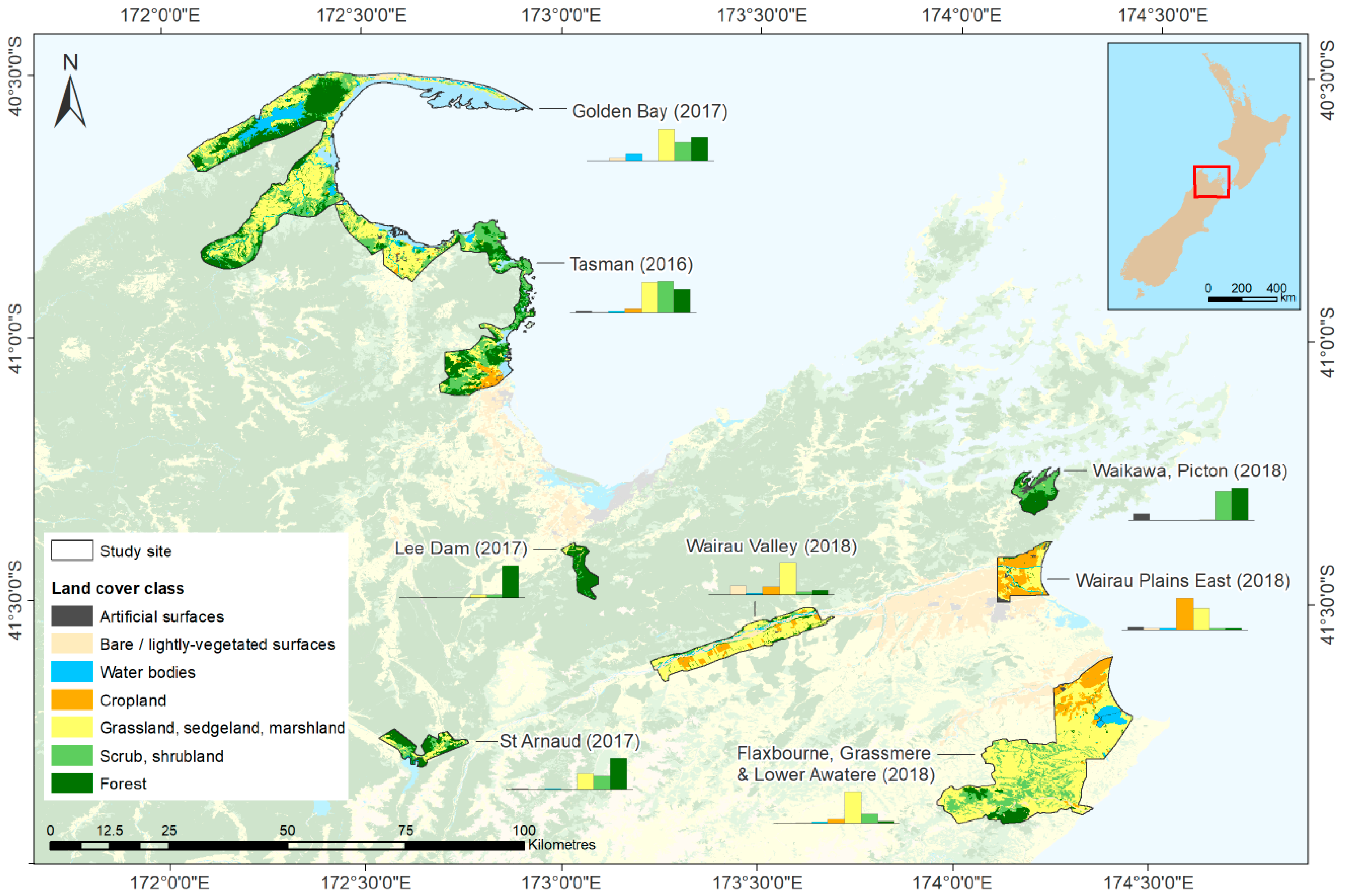
Since 2016, the New Zealand government mapping agency, Land Information New Zealand (LINZ), has published online a growing collection of 1 m resolution DTMs derived from airborne LiDAR topography surveys, providing ideal reference data for our purposes. Of the available surveys, three of the most recent were selected, comprising a total surveyed area of approximately 1560 km2 spread across eight survey sites in the Marlborough and Tasman regions (in the north of New Zealand’s South Island). These survey sites are mapped in Figure 2, with reference to their underlying land cover classes.

Figure 2.
The eight LiDAR surveys used as study sites (South Island, New Zealand), with reference to underlying land cover classes (based on the Land Cover Database v5.0 published by Manaaki Whenua/Landcare Research in 2020).
A wide variety of datasets covering these study sites was collected and processed for input to the machine learning models, comprising topography data from three different global products, supplemented by free, globally-available datasets of potential relevance to the vertical biases targeted here (primarily describing vegetation and built-up areas). While not all were eventually used (for reasons noted in Section 3.2), they are each presented briefly in the following sections, with Table S1 (Supplementary Materials) listing which were found to be useful model inputs.
The SRTM product was selected as the base DEM to be corrected (for reasons outlined in Section 2.1.3), so all other spatial inputs (including the reference topography data) were resampled so as to match the SRTM grid resolution and alignment over the study sites. All spatial processing was run using Geospatial Data Abstraction Library (GDAL) command-line utilities (version 3.0.2), applying median resampling for higher-resolution continuous data (reference topography data), cubic splines for all other continuous data (e.g., multi-spectral imagery), and nearest-neighbour resampling for categorical data (e.g., land cover classes).
Given that the raw data collection periods for the various topography datasets are so far apart in time (with raw data for SRTM collected during 11–22 February 2000, while the LiDAR surveys were flown at various times between December 2016 and September 2018), we have filtered input data to reflect conditions at the time of each survey (where possible).
2.1. Topography Data
Regardless of the machine learning algorithm used, the model must be provided with both the DEM to be corrected (input topography) and a higher-quality DEM that provides the target for that corrective process (reference topography). As noted above, we used LiDAR-derived DTMs published by LINZ as the reference data. A range of free, global DEM products was considered for the input data, with SRTM eventually selected as the primary input.
2.1.1. Reference Topography Data
All high-resolution DTMs published by LINZ were reviewed to find the most suitable surveys for this study, with the main criteria being a high LiDAR point density (considered more likely to penetrate vegetation and record the true ground elevation), a satisfactory vertical accuracy verification (noting that these were not available for all surveys), highly heterogeneous landscapes (especially in terms of elevations and land cover classes), and flood susceptibility (assessed based on hazard maps published by the National Institute of Water and Atmospheric Research [39]).
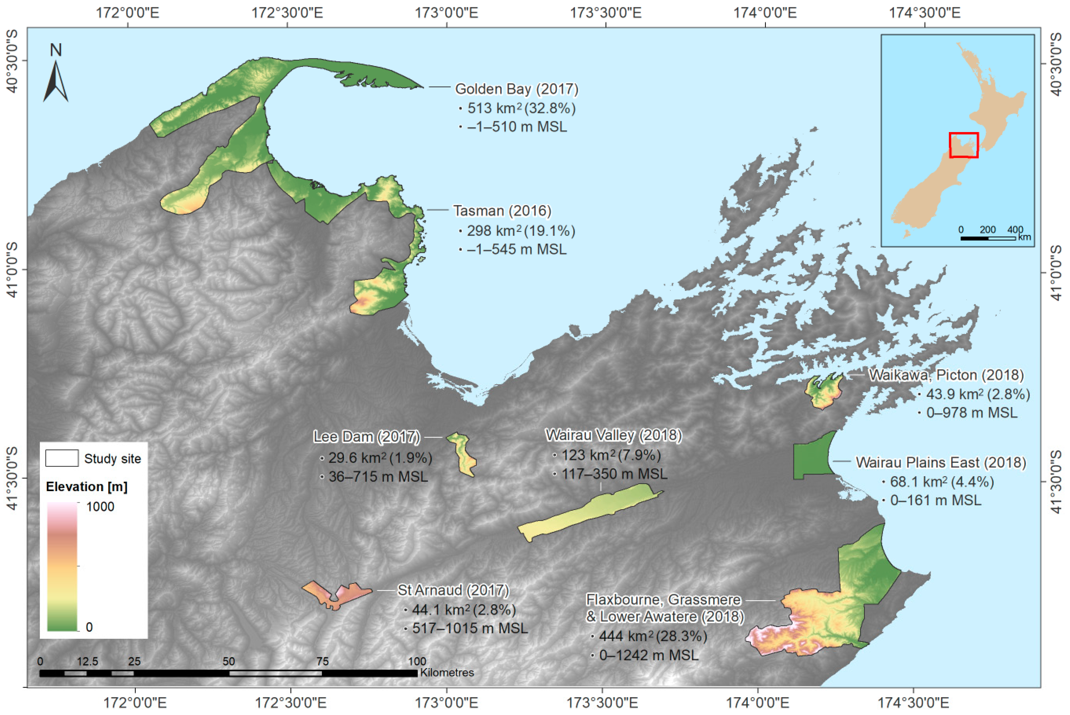
Based on these criteria, the DTMs derived from three of the most recent LiDAR surveys (2016–2018) were sourced from the LINZ Data Service (https://data.linz.govt.nz; CC-BY-4.0 license), and processed for inclusion in the modelling. These comprise eight different sites, for which the point density specification ranged between 2–3 points/m2, and independent verifications of vertical accuracy reported differences of 0.026–0.073 m for each site (in terms of root mean square error), based on 2130 field survey test points [40,41,42,43]. As shown in Figure 3, the eight sites available include coastal and inland areas, covering elevations ranging from 0 to 1242 metres above mean sea level.
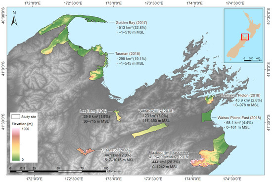
Figure 3.
The eight LiDAR-derived DTMs used as reference topography data.
It is noted that the topography data published by LINZ are provided with reference to the NZVD2016 vertical datum (based on the NZ Geoid 2016 model). In order to be consistent with the other topography datasets, these were transformed to the Earth Gravitational Model 1996 (EGM96) during the resampling step.
2.1.2. Input Topography Data
As summarised in Table 1, the three freely-available, global DEMs considered in this study all have a horizontal resolution of 1 arc-second (approximately 23 m at these latitudes) and differ primarily in terms of their data collection period and the method used to develop them.

Table 1.
Summary of the free, global Digital Elevation Models (DEMs) considered in this study.
For each DEM, a range of derivatives was also prepared, comprising slope, aspect, roughness, Topographic Position Index (the difference between a given grid cell and the mean of its surrounding cells) [44], and Terrain Ruggedness Index (the mean difference between a given grid cell and its surrounding cells) [44], as a way of incorporating some information about each cell’s neighbourhood.
2.1.3. Selection of Base DEM
While all of the free DEMs listed above were used for the modelling, it was necessary to select one as the “base” DEM, with all other datasets resampled to match its resolution and grid alignment, in order to develop spatially-consistent inputs for the machine learning models. To assess which DEM was most suitable for this, the reference topography data were resampled to match each of the three DEMs and then used to calculate the distribution of errors for each.
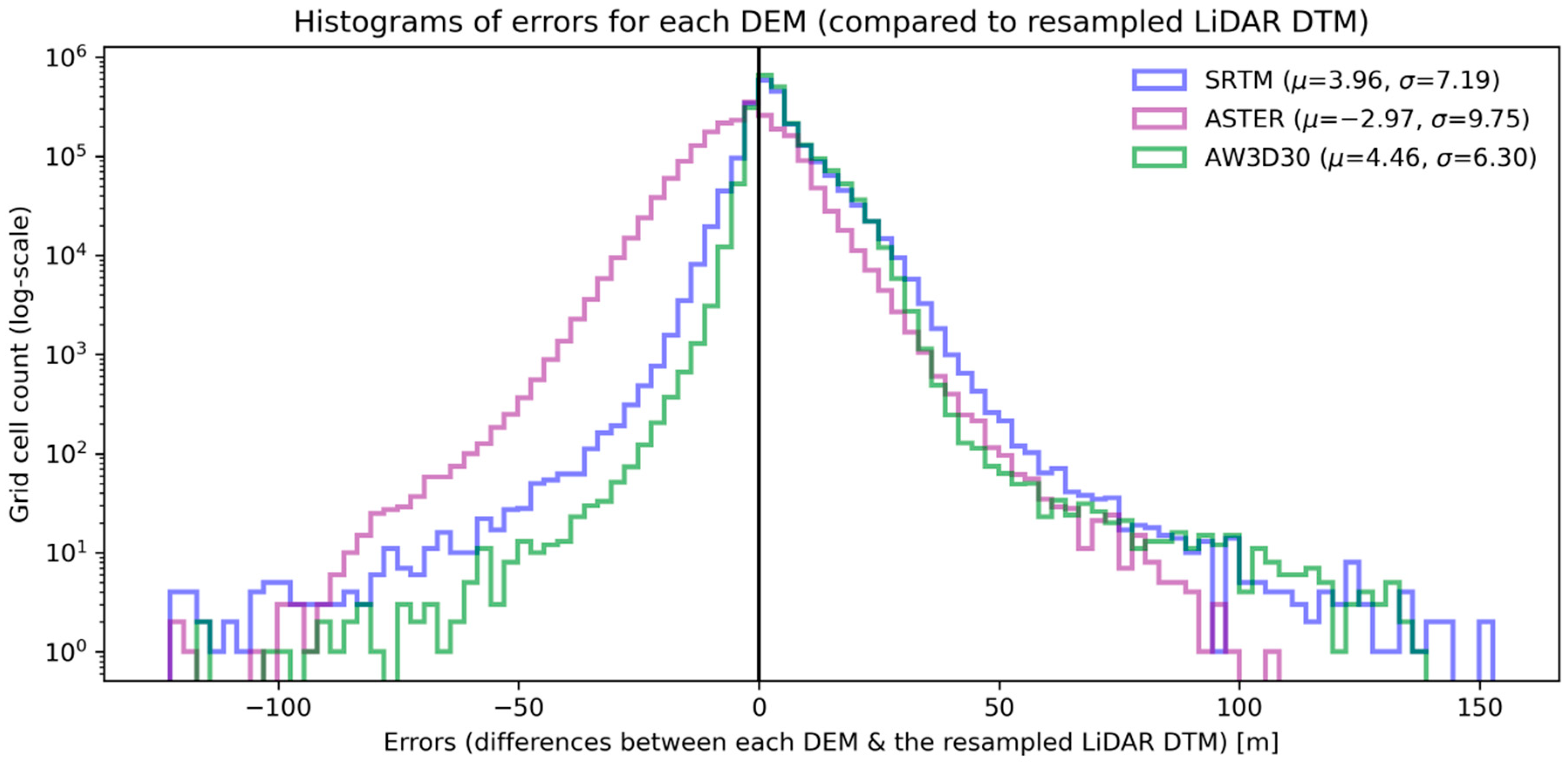
As shown by the histograms presented in Figure 4, the ASTER DEM had the widest distribution of errors across these areas, while the SRTM and AW3D30 DEMs were comparable (SRTM showing a smaller mean error but a wider spread of error values than AW3D30). We decided to use SRTM as the base DEM, primarily due to the relatively narrow temporal period during which its raw data were collected, which allows for the targeting of input data (especially multi-spectral imagery) to describe conditions on the ground at that particular point in time.
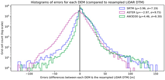
Figure 4.
Distribution of errors for each DEM (based on the resampled reference topography data), with means and standard deviations noted in the figure legend.
2.2. Multi-Spectral Imagery
Multi-spectral imagery from three different sources were processed in order to describe the prevailing land cover conditions in the study sites at the time of both the SRTM data capture (using Landsat 7 imagery) and each LiDAR survey (using Landsat 8 and Sentinel-2 imagery). This is visualised in Figure 5, showing the availability of multi-spectral imagery from each mission at the time of each topography data capture.

Figure 5.
Multi-spectral images were selected to represent conditions at the time of the SRTM data collection (using Landsat 7) and the LiDAR surveys (using Landsat 8 and Sentinel-2).
The three multi-spectral imagery sources considered in this study are briefly summarised in Table 2, generally showing a trend of increases (over time) in both the number of spectral bands available and the spatial (horizontal) resolution of each satellite’s imagery.

Table 2.
Summary of the multi-spectral imagery sources used in this study.
For each set of multi-spectral imagery, cloud-free composites were developed for each band by collecting a stack of overlapping images covering each study site (from multiple overpass dates), masking out any pixels judged to be problematic (on the basis of the quality assessment raster provided with each input image, usually relating to clouds or cloud shadows), and extracting the medians of the valid pixels available. For the two Landsat collections, an input window of four months (centred on the relevant topography data acquisition period) was selected, as this ensured sufficient cloud-free pixels for a clear image while still representing conditions on the ground during each period of interest. However, significant artefacts were found in the Sentinel-2 composites regardless of the input window used (a known issue relating to the scene classification mask currently used [45]), so Sentinel-2 products were excluded from the subsequent modelling.
In addition to these sets of cloud-free composite images (for each band of the Landsat collections), 11 spectral index products were also derived, comprising the Normalised Difference Vegetation Index (NDVI), Enhanced Vegetation Index (EVI), Advanced Vegetation Index (AVI), Soil Adjusted Vegetation Index (SAVI), Modified Soil Adjusted Vegetation Index (MSAVI), Bare Soil Index (BSI), Shadow Index (SI), Normalised Difference Moisture Index (NDMI), Modified Normalised Difference Water Index (MNDWI) [46], Automated Water Extraction Index (AWEI) [47] and Normalised Difference Built-up Index (NDBI) [48]. It was anticipated that the vegetation and built-up indices would help to predict the two largest expected causes of bias (vegetation and buildings), while the water indices may help with further refinements (for example, a grid cell found to be wet very often is likely to be at least slightly lower than its drier neighbours).
2.3. Night-Time Light
Night-time light imagery covering the two primary periods of interest was also included, based on its identified value as a proxy for economic and/or urban development [49,50,51], which may be relevant to building biases. Conditions at the time of the SRTM data capture are represented using imagery from the Defense Meteorological Satellite Program’s Operational Linescan System (DMSP/OLS), while those representing the general period of the LiDAR surveys are based on imagery from the Suomi National Polar-orbiting Partnership’s Visible Infrared Imaging Radiometer Suite (Suomi NPP/VIIRS).
2.4. OpenStreetMap Derivatives
The potential value of digitised features derived from the OpenStreetMap project was explored, although it was later found that they did not contribute significantly, at least in the study areas considered here. Building footprints and primary road networks were downloaded using the OSMnx Python package (version 0.11.1) [52], and rasterised for input to the modelling workflow.
Given the significant impact that bridges often have when using free DEMs for hydrological applications [53,54], we attempted to explicitly identify these by extracting lines wherever major roads were found to intersect river banks, and then rasterising these features based on the same grid resolution and alignment used for the other inputs.
2.5. Other Global Data Products
Three other potentially-relevant datasets were identified which satisfied the requirements of being both freely available and also having global (or near-global) coverage: a forest canopy height map (30 arc-second resolution, approximately 695 m at these latitudes) [55], a vegetation density map (1 arc-second resolution, approximately 23 m) [56], and a map of surface water occurrence percentage (1 arc-second resolution, approximately 23 m) [57]. All three products are based on data collected in (or shortly prior to) the year 2000, meaning they are more relevant to conditions at the time of the SRTM data collection (rather than the more recent LiDAR surveys).
3. Method
The datasets discussed above were processed (in particular, resampling each to match the geographic projection, horizontal resolution and grid alignment of the SRTM DEM) and then divided into training, validation and testing sets. A preliminary random forest model was used to filter out unhelpful features using Sequential Forward Floating Selection (SFFS), reducing the initial set of 66 features to a more manageable 23, which reduced both model variance and training times.
Three different types of machine learning model were then trained, including some hyperparameter tuning for each (adjusting those model parameters which aren’t learnt during training but must be manually defined when the model is initialised). It is likely that further improvements are possible with extended hyperparameter tuning efforts. Importantly, the same training/validation/testing datasets were used throughout (in each case including only the 23 selected features), to ensure comparability between the three sets of results.
All data processing, model development and result visualisation was coded using the Python programming language (version 3.7), with particularly important packages noted in the sections below and all code fragments shared in the online repository listed under Supplementary Materials. The maps presented in Figure 2, Figure 3, Figure 6 and Figure 9 were prepared using ArcGIS 10.4.1 (ESRI, Redlands, CA, USA).
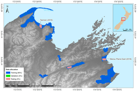
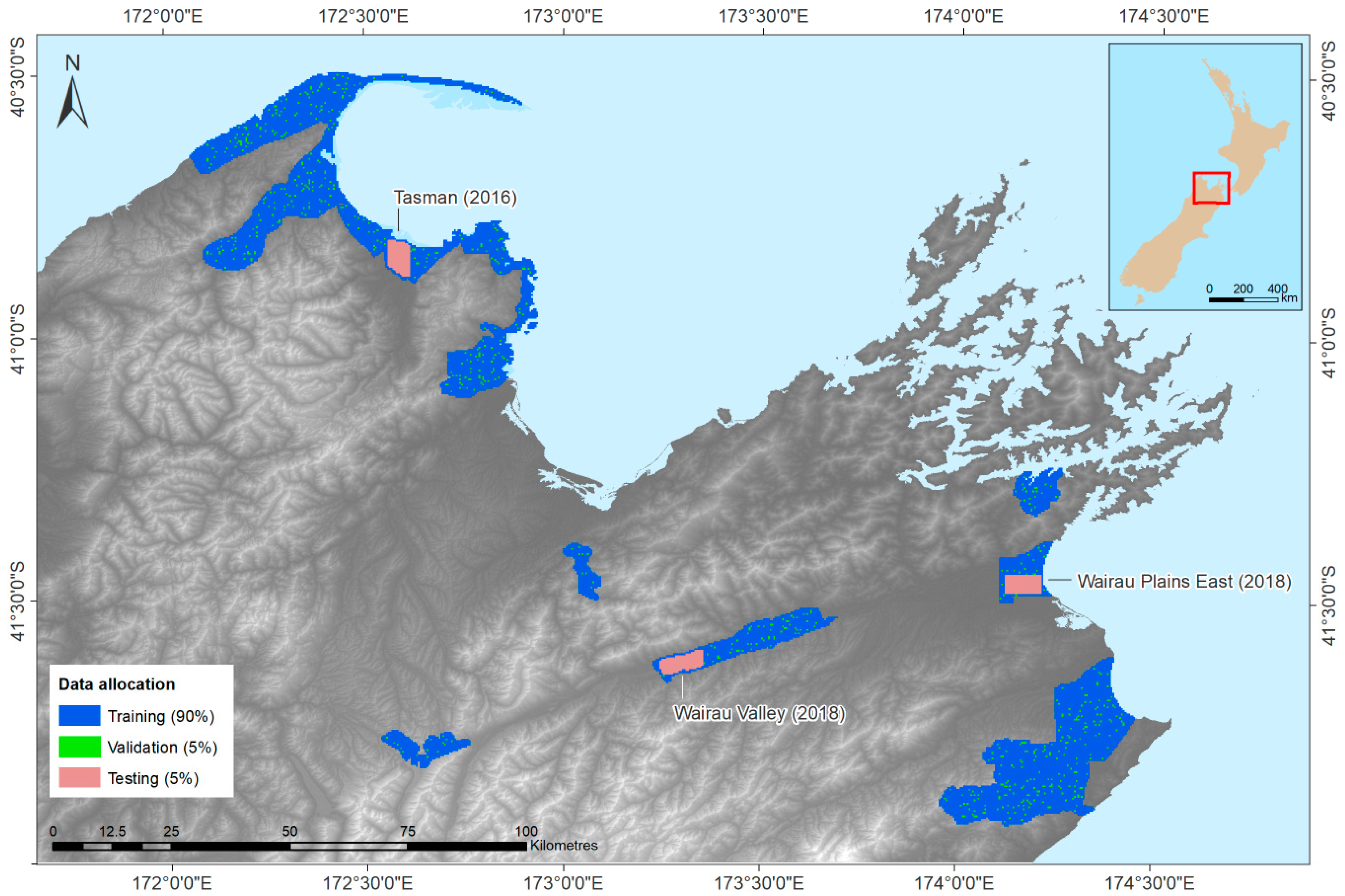
Figure 6.
Image patches derived based on LiDAR-derived DTM coverage and their allocation for training (90%), validation (5%) and testing (5%) purposes.
3.1. Allocation of Available Data to Training, Validation and Testing Sets
Regardless of the machine learning algorithm used, it is important to set aside some of the available data before training, in order to test how well each trained model performs on data that it hasn’t yet encountered (in other words, whether the model generalises well by learning genuine relationships, rather than simply memorising the training data provided to it). It is also useful to set aside a validation (or development) dataset, which is used when tuning the hyperparameters (model parameters which aren’t learnt during training but must be manually defined).
As shown in Figure 6, we split up the available data by first allocating three floodplain areas for testing purposes (red patches, 5%), since this is the primary application intended, while the remaining survey zones were pooled and then randomly divided into training (blue, 90%) and validation (green, 5%) “patches” (grids of neighbouring pixels). The use of these patches reflects the input requirements of the FCN model (since it learns from intact images, rather than individual pixels). In order to ensure comparability, the same data allocation was used for the RF and DCN models, with each set of patches flattened to vectors before being fed into those models.
3.2. Feature Selection Using Sequential Forward Floating Selection (SFFS)
Considering all datasets processed and the additional derivatives prepared, a total of 66 features/variables were available for input to the machine learning models. At least some of these are likely to be irrelevant (i.e., having no relation to the vertical biases we are trying to predict) and will result in “over-fitting” if retained (where the model fits to random noise in the training data, limiting its ability to generalise to new data). In addition, having many input features slows down the training process, which is particularly significant during the iterative process of hyperparameter tuning.
To filter out unhelpful features, the mlxtend Python package (version 0.17.2) was used to run a Sequential Forward Floating Selection (SFFS), using small random forest models (10 trees) and a random sample of the training dataset (10%) in order to make the search tractable. In an iterative process considering an increasing number of allowed features, a sequence of random forest models were trained, each searching for the optimal feature subset given the prescribed size (using a greedy search algorithm that can both add and drop features, based on a cross-validation score). As shown in Figure S1 (Supplementary Material), only marginal improvements were found beyond a feature subset size of 23 (out of 66), at the cost of increasing training times and model variance. For each type of machine learning model considered here, these same 23 features were used for all subsequent modelling, enabling direct comparisons between each model type. A full list of all 66 features considered is provided in Table S1 (Supplementary Materials), indicating the 23 features selected.
3.3. Hyperparameter Tuning Using Sequential Model-Based Optimisation (SMBO)
In addition to those machine learning model parameters which are adjusted during the training process, there are other parameters–known as “hyperparameters”–which are not learnt during training and must instead by defined beforehand by the modeller. Finding the optimal configuration for these hyperparameters can be a difficult and time-consuming task, becoming exponentially more so as the number of hyperparameters and/or their parameter spaces increase.
For the models trialled here, hyperparameters were tuned using the sequential model-based optimisation (SMBO) approach implemented in the optuna Python package (version 1.3.0) [58]. This is a Bayesian optimisation technique which uses information from past trials to decide which hyperparameter values to try next, making it more efficient than the more common grid or randomised search approaches. For each trial in this sequential process, a new model was initialised with a different set of hyperparameter values, fitted to the training data and then evaluated in terms of its performance on the validation data (as presented in Section 3.5).
3.4. Machine Learning Algorithms Tested
Three machine learning algorithms were tested: a random forest (a well-established and widely-used approach to non-linear regression, intended as a baseline against which the other approaches will be assessed), a densely-connected neural network (similar to those used in the most recent research efforts on this problem [5,21]), and a fully-convolutional neural network (an innovative approach not yet applied to this task, which is capable of analysing intact images and learning from spatial context at various scales).
The following sections provide a brief overview of the three models developed (including their performance on the validation dataset, as part of the hyperparameter tuning process), with a more detailed summary of model architecture and hyperparameters available in Section S2 of the Supplementary Materials. In Section 4, each of the final trained models is assessed based on its performance on the test dataset, which was kept aside during training (i.e., completely unseen data), as an indication of how well each can generalise to new data.
3.4.1. Random Forests (RF)
Random forest regression is an ensemble approach, in which multiple classifying decision trees are trained using bootstrap samples of the available training data (of the same size as the available dataset but resampled with replacement for each tree) and final predictions are simply the average of predictions made by each decision tree within the forest.
Models were built using the scikit-learn Python package (version 0.22), with hyperparameters tuned so as to minimise the validation error while avoiding over-fitting. A relatively small model (consisting of 250 trees) was found to perform best, with the maximum number of features considered for each individual tree limited to 11 (slightly more than the default recommendation for random forest regression, which is a third of all available features [59]).
3.4.2. Densely-Connected Neural Networks (DCN)
The second machine learning algorithm tested here is of the same type used in the two most recent studies exploring this issue [5,21]–a densely-connected neural network, sometimes referred to as a multi-layer perceptron. This type of model consists of an input layer (with 23 neurons in this case, corresponding to pixel values from each of the selected input features), an output layer (one neuron, the prediction of the correction required for that particular pixel), and a variable number of hidden layers in between, with each neuron connected to every neuron in the two layers immediately preceding and succeeding it (as suggested by the name).
As shown in Figure 7, three hidden layers were selected for this model, respectively containing 3074, 4089 and 1222 neurons (the optimal values found during hyperparameter tuning). Each of the hidden layers uses batch normalisation (normalising the values of each layer’s neurons before activation) and dropout (randomly switching off a certain proportion of a layer’s neurons) to combat overfitting and speed up learning [60]. All neural network models (including the convolutional networks described in Section 3.4.3) were developed using the tensorflow Python package (version 2.1.0) and run using a NVIDIA GeForce GTX 1080 GPU.

Figure 7.
Architecture of the densely-connected neural network used in this study.
3.4.3. Fully-Convolutional Neural Networks (FCN)
Convolutional neural networks are a distinct subset of neural network developed specifically for image processing and computer vision tasks, designed to learn from spatial patterns in the input imagery (regardless of where in the image those patterns appear), at a variety of different scales [61,62,63]. In other words, they learn not only from the input features available for a given pixel or grid cell, but also from those of its neighbours, accounting for potential spatial relationships in that neighbourhood. This has made them very successful in image classification and segmentation tasks [36,37], including some applications involving satellite imagery [64,65,66]. However, to the best of our knowledge they have not yet been applied to the task of topography bias correction. The main contribution of the research presented here is therefore to explore their potential and benchmark their performance against two other, more commonly used machine learning approaches.
We base our convolutional network on the U-net model architecture developed by Ronneberger et al. [36] for image segmentation, which uses approximately symmetric contracting (down-sampling) and expanding (up-sampling) convolutional stages, with results at each spatial scale combined so as to learn patterns at a variety of scales. The network architecture used here is presented in Figure 8, involving one fewer contraction/expansion step than in the original U-net model, based on the assumption that the present task does not require quite as much spatial context as the original segmentation application (given the coarse horizontal resolution of our input data).
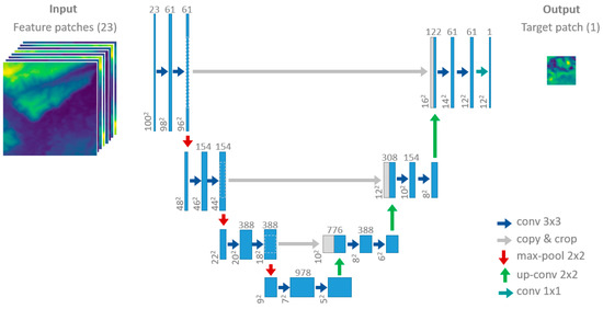
Figure 8.
The FCN architecture used here, a simplification of the U-net model developed by Ronneberger et al. [36], showing how the model is able to learn at different spatial scales.
Importantly, while most convolutional neural networks include a densely-connected layer right at the end (usually for classification purposes), the U-net model does not involve any densely-connected layers at all (hence the “fully-convolutional” label). This allows the network to handle different input image sizes and to generate intact images (rather than single values or labels). As was the case for the DCN model, both batch normalisation and dropout are used for regularisation (reducing over-fitting) and to speed up learning [60], with Gaussian dropout found to be slightly more effective for the FCN [67].
Given that FCNs learn from intact images rather than individual pixels, their input requirements are quite different to those of the RF and DCN models. We addressed this by generating contiguous “patches” of target data (the elevation corrections required) consisting of 12 × 12 grid cells, as well as sets of corresponding feature patches (for all 23 selected features) with a larger spatial extent (100 × 100 grid cells), to ensure that all grid cells in each target patch could learn from an equally large neighbourhood (even those along the edges of a target patch). Figure 9 presents an example of such a target patch and its corresponding feature patch from the Wairau Valley survey zone.
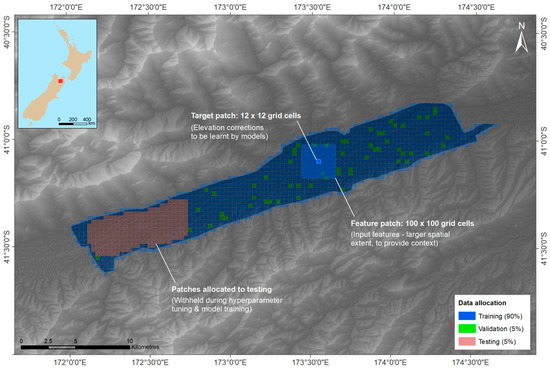
Figure 9.
An example of a target patch (12 × 12 cells) and its corresponding feature patch (100 × 100 cells) in the Wairau Valley survey zone, illustrating the spatial context provided to the FCN.
Although the FCN’s capacity to learn from intact images is likely to be an advantage in terms of the spatial patterns it can learn, all input image patches must be complete (i.e., no missing pixels). This means that a significant number of pixels along the boundaries of each LiDAR survey zone (those not part of a complete patch) are not used by the FCN model. We explored the use of data augmentation to supplement the training data that remained [33,63], applying horizontal and vertical flips as well as 90° rotations to each feature and target patch in the training data (but not to the validation or testing datasets). An example of the flips explored for a particular feature patch is presented in Figure 10, showing how it might allow the model to learn from different orientations of the spatial patterns present in the available data. However, no improvements were found (even if we excluded input features explicitly related to direction, such as topographical aspect) and data augmentation was eventually not used at all.

Figure 10.
An example of the flip data augmentation approaches explored to expand the available training data, involving horizontal and/or vertical flips.
3.5. Evaluating Model Architecture and Hyperparameter Values Using the Validation Dataset
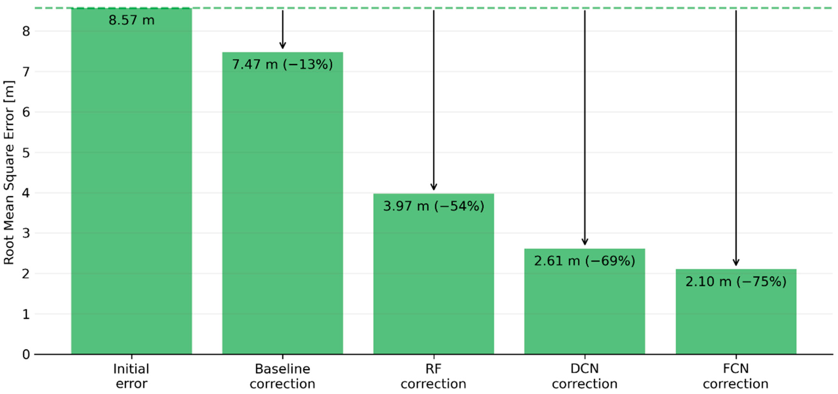
Throughout the hyperparameter tuning process described in Section 3.3, a wide variety of model architectures and hyperparameter values was explored, with each new model configuration trained on the same set of training data (90% of all data available) and then evaluated in terms of how well it predicted the validation dataset (5%). Targeting validation (rather than training) performance helps to avoid overly complex models which would go beyond the genuine relationships present and fit to random noise in the training data. As shown in Figure 11, the initial root mean square error (RMSE) present in the validation dataset (8.57 m) was reduced somewhat (13%) by what we’ve termed the baseline correction (simply subtracting the mean vertical bias observed in the training data from each SRTM grid cell), while all of the machine learning models explored achieved significantly higher improvements (ranging between 54–76%). As might be expected, the FCN’s capacity to learn patterns at the neighbourhood as well as the pixel scale seemed to enable it to outperform the other models.

Figure 11.
Root mean square error for the validation dataset, showing the initial error and the impact of corrections based on a simple vertical shift and the three machine learning models tested here.
4. Results
For a more rigorous assessment of how well each topography correction model has generalised (i.e., how well it performs on data not used at all during the training process), the following sections present results from the three test datasets (similarly sized areas within the Wairau Plains East, Wairau Valley and Tasman LiDAR survey zones). These were allocated as test zones (during the process outlined in Section 3.1) as they each contain a significant river channel and extensive flood-prone areas [39], making them particularly interesting from a flood hazard perspective.
A variety of different metrics are used for this assessment, illustrating each model’s overall performance (in terms of impact on root mean square error and the distribution of residual errors, when compared with the LiDAR-derived DTM) as well as for more targeted flood applications (looking at derived cross-sections across rivers and their floodplains).
4.1. Overall Performance
To reiterate, each of the three models trialled here was fitted to the training dataset (learning model parameters such as weights), with the validation dataset used in an iterative process to fine-tune the model hyperparameters (those parameters not learned during training but pre-selected by the user). As a final assessment, each trained model was then used to make predictions for the test dataset (as yet unseen by any of the models), for an indication of how well each is able to generalise to new locations.
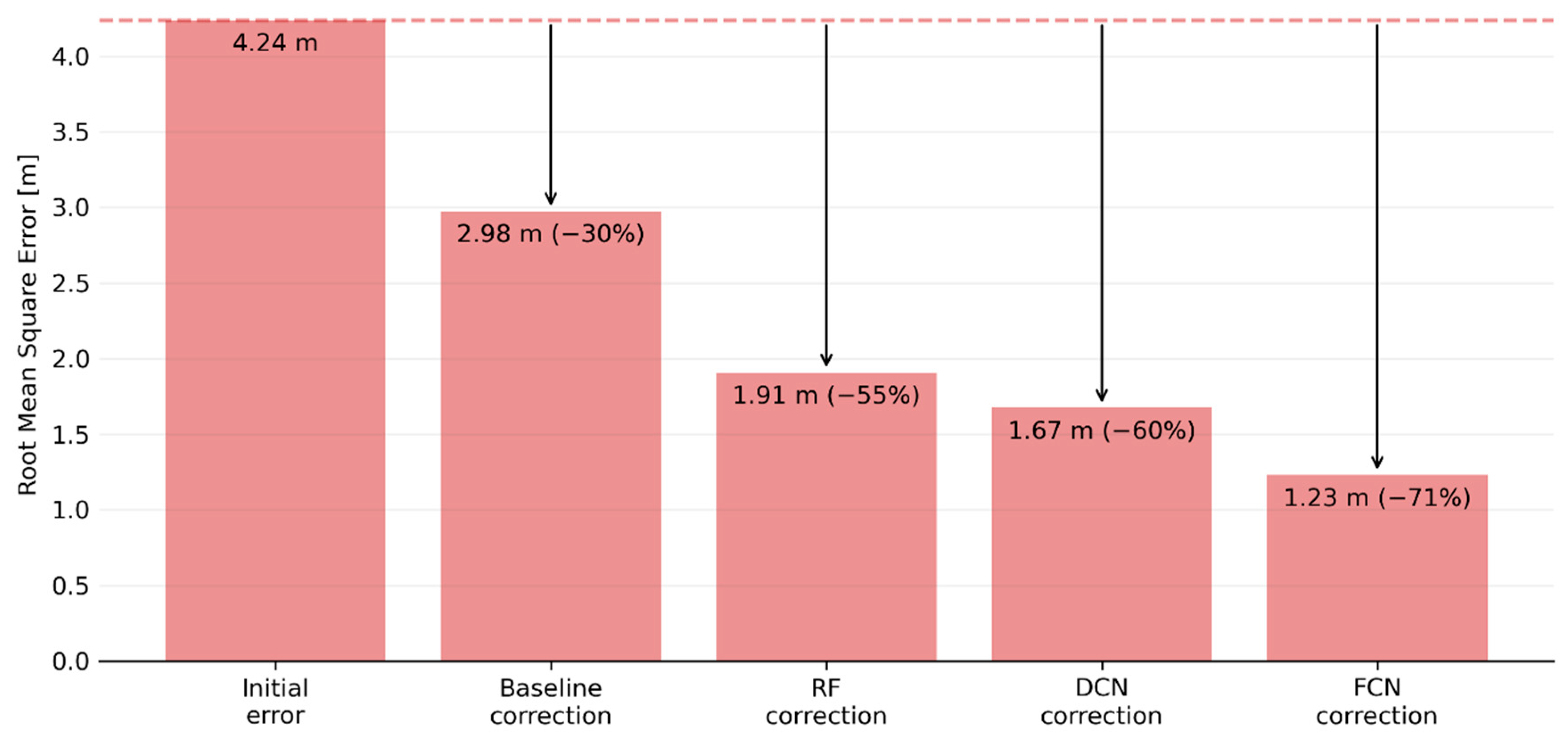
Figure 12 summarises these results in terms of root mean square error (RMSE), showing the initial RMSE present in the pooled testing dataset (4.24 m), and the extent to which this was reduced using a baseline correction (simply shifting all elevations by the mean vertical bias observed in the training data) or the predictions generated by each model. A similar pattern to the validation results is seen here, with the FCN (which reduced RMSE by 71%) outperforming the DCN (60%) and RF (55%). Importantly, performance on the test data is fairly similar (in terms of RMSE reduction) to the validation results, which suggests that the models have not over-fitted and are generalising reasonably well.
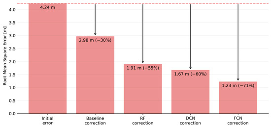
Figure 12.
Root mean square error for the test dataset, showing the initial error and the impact of corrections based on a simple vertical shift and the three machine learning models tested here.
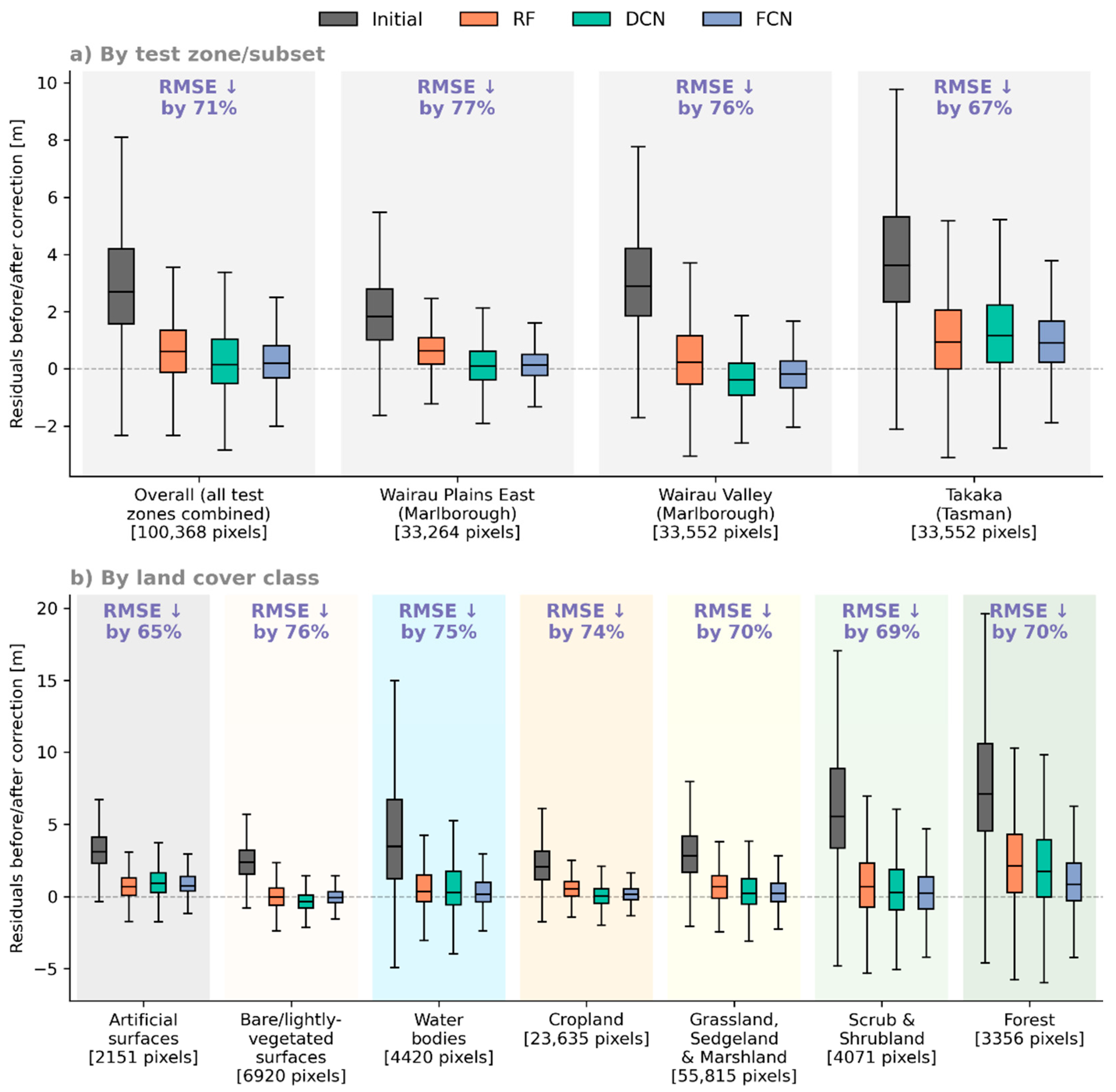
Figure 13 uses boxplots to visualise the distribution of residuals before and after applying the corrections predicted by each model, filtering these according to (a) test zone and (b) land cover class (based on the same Land Cover Database introduced earlier, resampled to match the SRTM grid). For each of these filtered subsets, the label at the top shows which model achieved the highest reduction in RMSE (indicated by text colour) and the percentage reduction achieved. As shown, we found that the FCN consistently achieved the best results (in terms of both the highest RMSE reduction and the narrowest distribution of residuals), across all of the test zones and land cover classes considered here.
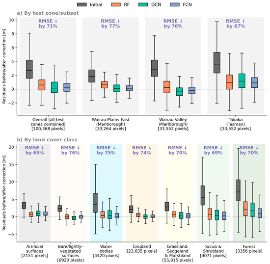
Figure 13.
Boxplots showing test residuals before and after corrections, filtering the pooled test data according to (a) test zone and (b) land cover class, with the label above each set of boxplots indicating (by colour) the best-performing model and the RMSE reduction it achieved.
Looking at the residuals by underlying land cover class, the largest initial errors were found in areas covered by forest, scrub or shrubland, and water bodies (likely due to the presence of relatively thick vegetation often found along riverbanks). Of all classes, the least effective corrections are seen for artificial surfaces (built-up areas, roads, etc.), which likely reflects the relatively low prevalence of this class in the training (1.1%) and validation (1.0%) data, as well as the difficulty in estimating the height of a building based primarily on the surface reflectance characteristics of its roof.
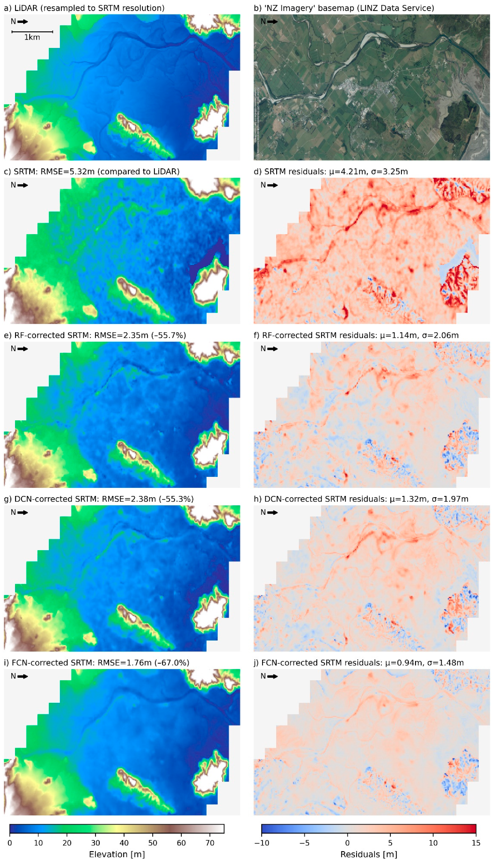
The maps presented in Figure 14, Figure 15 and Figure 16 provide a spatial overview of the DEM corrections achieved in each of the three test zones, in terms of predicted topography and associated residuals (judged against the resampled LiDAR data). Each map also shows the resampled LiDAR survey data (a), satellite imagery (b) and the original SRTM data, as visual references in evaluating the corrections made. With regards to potential flood modelling applications, it is especially interesting to see the extent to which river branches (significantly obscured by vegetation in the original SRTM) have been resolved in each zone. The FCN proved particularly effective at removing vegetation-related features that would otherwise block flow across the floodplains, such as the diagonal lines visible in the south-east of the Wairau Valley zone (wind-break planting between fields). More generally, the corrections made by the FCN have also filtered out much of the random “speckle” noise present in the original SRTM data.
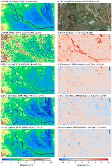
Figure 14.
Maps of the Wairau Plains East test zone, showing (a) resampled LiDAR DTM, (b) reference satellite imagery, (c) original SRTM topography, (d) SRTM residuals, and corrected topography and residuals based on predictions using the RF (e,f), DCN (g,h) and FCN (i,j) models.
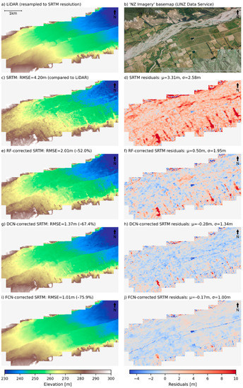
Figure 15.
Maps of the Wairau Valley test zone, showing (a) resampled LiDAR DTM, (b) reference satellite imagery, (c) original SRTM topography, (d) SRTM residuals, and corrected topography and residuals based on predictions using the RF (e,f), DCN (g,h) and FCN (i,j) models.
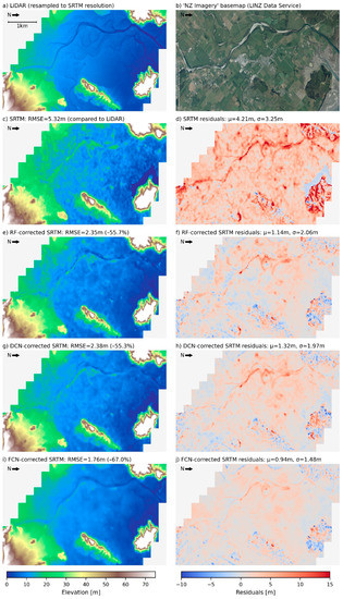
Figure 16.
Maps of the Takaka test zone, showing (a) resampled LiDAR DTM, (b) reference satellite imagery, (c) original SRTM topography, (d) SRTM residuals, and corrected topography and residuals based on predictions using the RF (e,f), DCN (g,h) and FCN (i,j) models.
4.2. Performance on Flood-Related Objectives
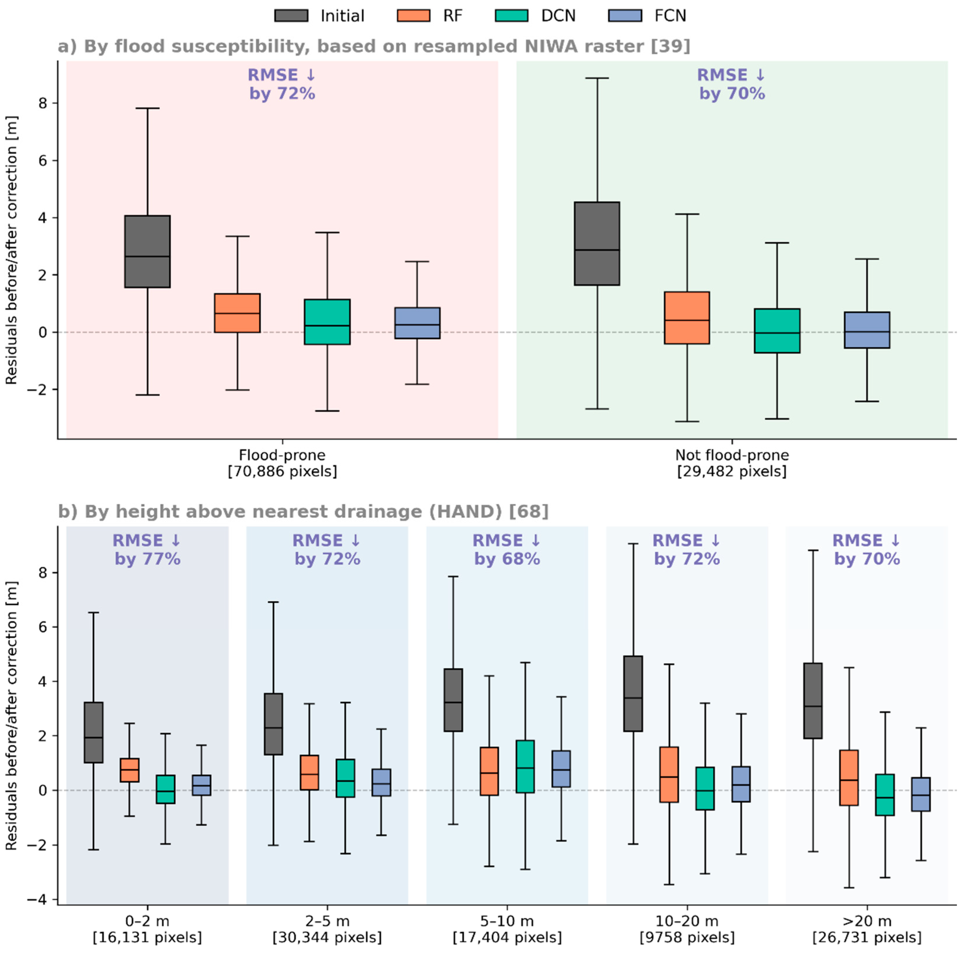
While flood hazard modelling using the various corrected DEMs is beyond the scope of this study, we made an initial assessment of performance on flood-related objectives by looking at test residuals according to flood susceptibility zone [39] and by deriving a map of Height Above Nearest Drainage (HAND) values [68]. As shown in Figure 17, performance across these different flood-related classifications did not vary greatly, with the possible exception of the lowest HAND range (grid cells for which the resampled LiDAR topography was within a 2 m vertical distance of the nearest drainage cell), where FCN corrections achieved a reduction in RMSE of 77% (compared to 71% more broadly).
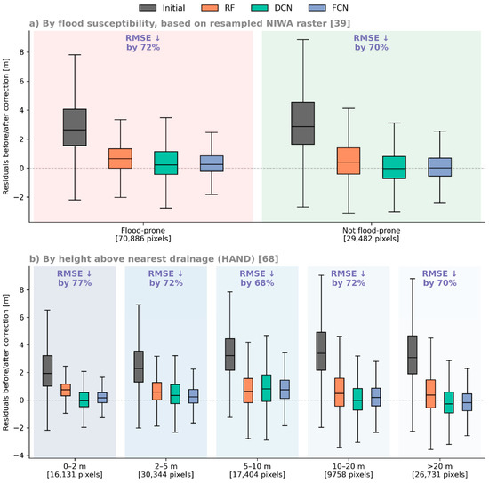
Figure 17.
Boxplots showing test residuals before and after corrections, filtering the pooled test data according to (a) flood susceptibility zone [39] and (b) HAND class [68], with the label above each set of boxplots indicating (by colour) the best-performing model and the RMSE reduction achieved.
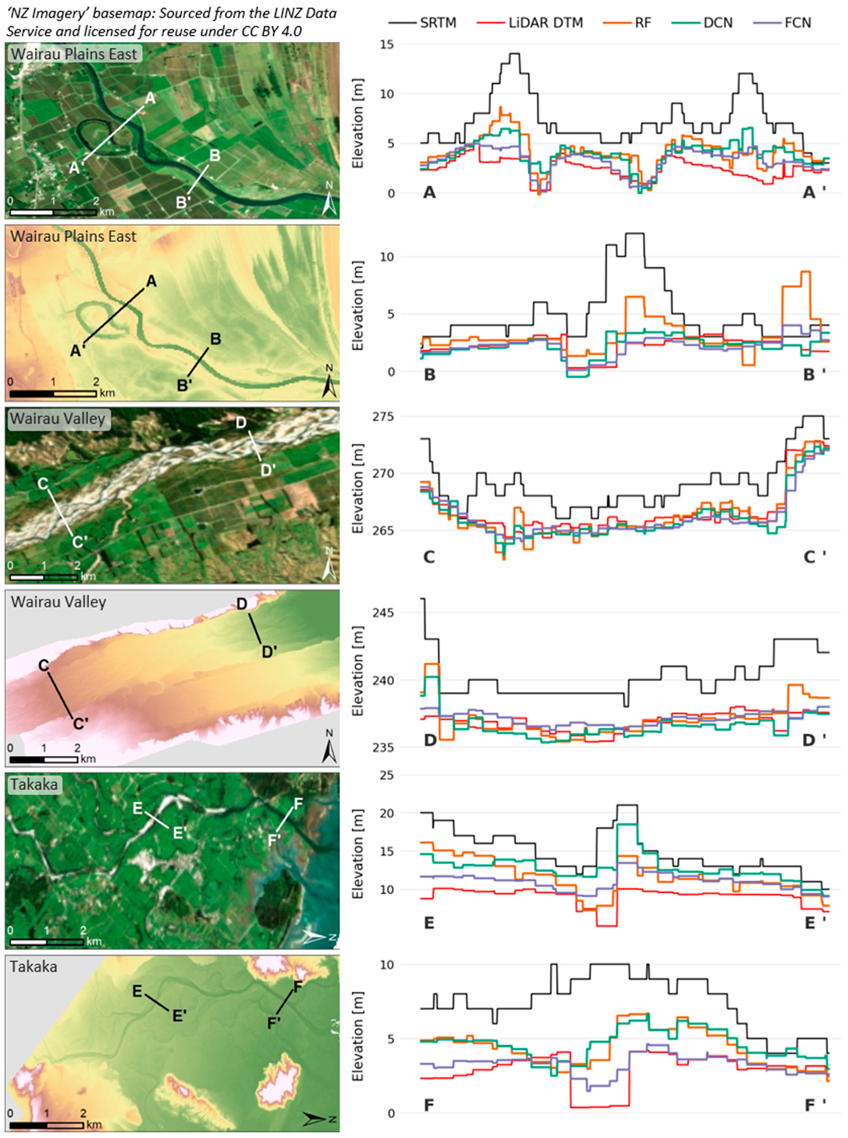
As an additional assessment of each model’s potential for flood modelling applications, two cross-sections were extracted along the main river branch and floodplain in each test zone, as shown in Figure 18. For each cross-section, the original SRTM elevations (black line) are compared to the reference LiDAR DTM (red line), as well as the three corrected datasets. The profiles extracted suggest that all models are reducing at least some of the vegetation bias, with particularly effective improvements achieved for elevations in or adjacent to the river. As for elevations within river beds, at least some of the cross-sections (particularly A to C) show the FCN-corrected profile (purple line) matching very closely with the minimum river elevation indicated by the LiDAR profile (red line), suggesting that this corrected topography may allow improved performance for hydrological applications such as the automated delineation of stream networks.
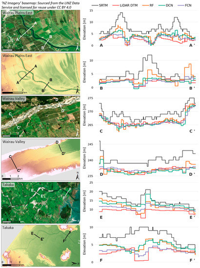
Figure 18.
A comparison of elevations for two river cross-sections taken in each test zone, showing the original SRTM, the resampled LiDAR DTM and the three corrected SRTM datasets.
5. Discussion
The results presented here suggest that machine learning techniques, in concert with a wide variety of remote-sensed datasets, are able to predict at least some of the vertical biases known to affect freely-available, global DEMs. Given the number of large-scale flood hazard assessments which continue to rely on these free topography data, being able to predict (and therefore correct) these biases would be a useful step towards more accurate flood hazard and risk modelling.
Of the three machine learning techniques tested here, performance was found to improve with increasing model complexity, with the simplest model (RF) reducing test RMSE by 55%, the more complex DCN outperforming that (60%), and the most complex model (FCN) going even further (71%). This is likely due to its ability to learn from spatial patterns at multiple scales, which represents a significant advantage over the other models, which learn on a pixel-by-pixel basis including only very rudimentary information about their spatial context (such as slope values).
Importantly, fairly similar results were observed for the validation error correction rates (e.g., 75% for the FCN), which suggests that all models have learnt from genuine relationships/patterns within the data that allow them to generalise reasonably well to new locations. In the following sections, potential issues relating to class imbalances (between training, validation and test datasets) are explored and the test results are discussed within the wider context of other published work in the field.
5.1. Discrepancy between Model Performance on Validation and Test Datasets
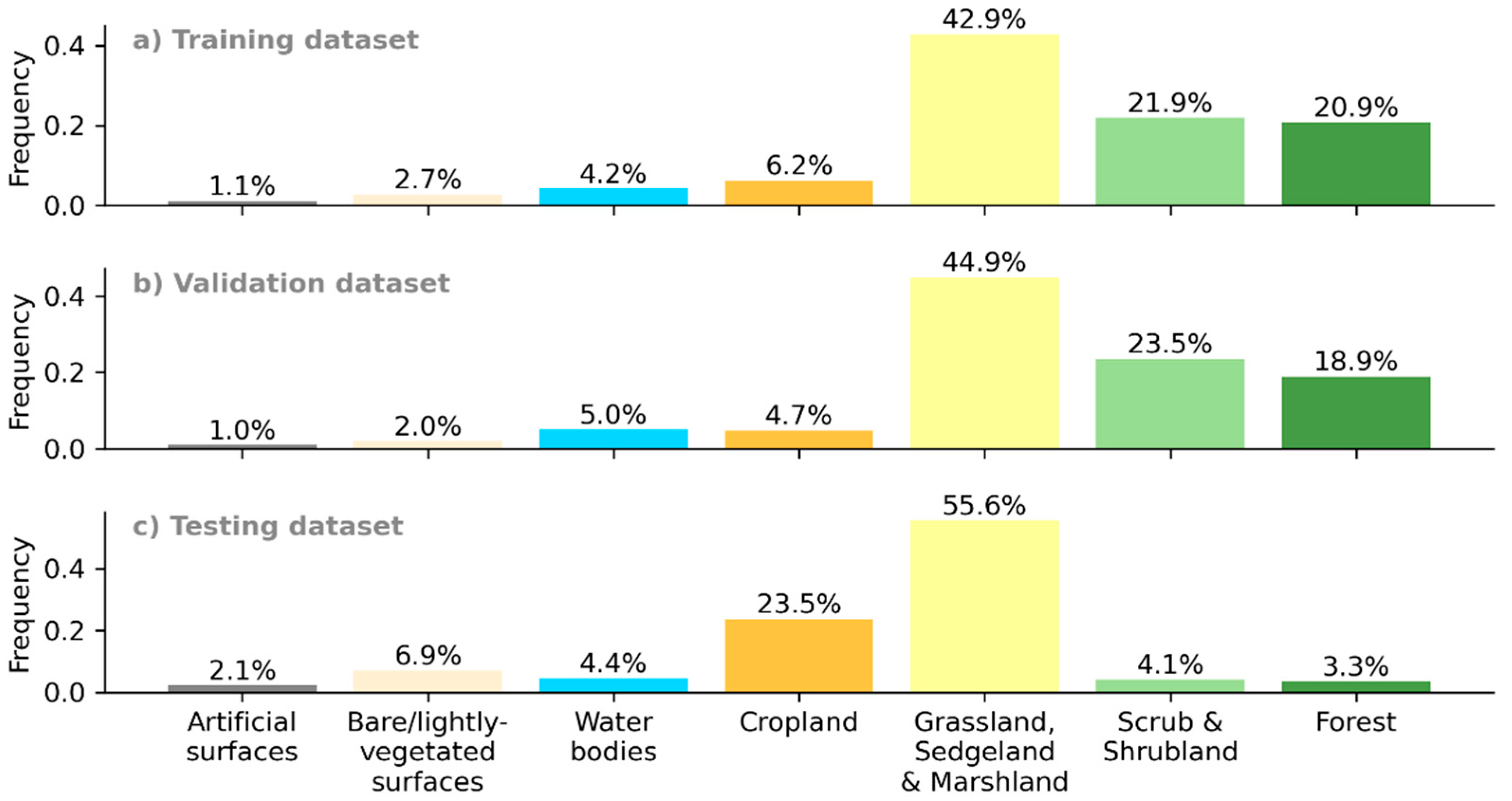
To explore possible reasons for the small discrepancies observed (between validation and test correction rates), we compared the distributions of land cover classes and topography across each of the zones (training, validation and testing). Figure 19 makes this comparison for underlying land cover classes, showing that the training and validation zones are very similar (as expected, given that they are random subsets of the same pooled survey zones), while the testing zones have some notable differences. The training and validation zones include relatively high proportions of scrub, shrubland and forest, meaning that all models will be biased towards learning how to predict errors in these types of areas (since these are some of the most common examples from which they extract patterns). By contrast, the testing zones have a lot more cropland and include a relatively high proportion of artificial and bare surfaces, neither of which were as common in the training or validation zones.
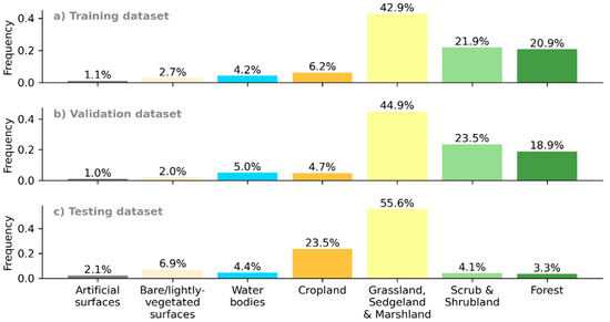
Figure 19.
Relative frequencies of each land cover class, in the (a) training, (b) validation, and (c) testing zones, with notable differences observed between the training/validation and test zones.
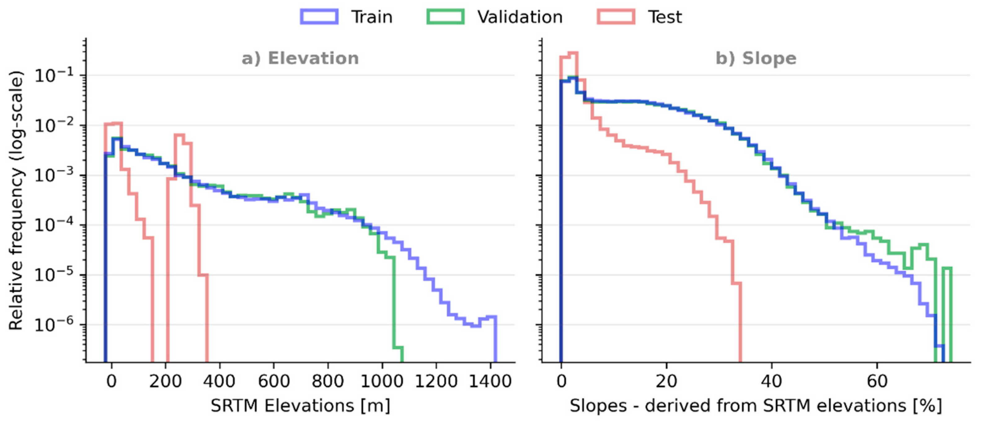
A similar pattern is observed for the distribution of SRTM elevations and derived slope values (Figure 20), with the training and validation datasets found to have much wider distributions than that of the testing data (which tend to be low-lying and relatively flat, reflecting the flood-prone areas selected as testing sites).
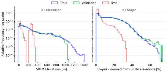
Figure 20.
Relative frequencies (log-scale) of (a) SRTM elevations and (b) derived slope values, in the training, validation, and testing datasets, showing notably different distributions for the testing data.
This raises important questions about the potential significance of class imbalances between the datasets used to develop the models and those covering their intended application area(s). Given the specific application targeted here (flood-prone areas), would model performance improve if the models were trained using only data from other flood-prone areas (noting that this would be a much smaller dataset, with models therefore more susceptible to over-fitting)? Or does exposure to a wider set of conditions (making full use of all available data, which are often limited), allow the models to learn additional patterns which help them generalise to new flood-prone areas?
Future work extending the research presented here might address these questions in two ways. One would be to develop a parallel set of models which are trained only on the subset of available training data judged to be in flood-prone areas, to assess the likely trade-off between closer dataset alignment (effectively forcing models to focus on patterns found in flood-prone areas) and the corresponding reduction in the training dataset size (which would increase the risk of over-fitting and potentially require the use of less complex model architectures).
Another approach to exploring this issue would be to set aside even more data for testing purposes, by sampling randomly from all available patches (just as was done for the validation dataset), as a complement to the manually-selected contiguous flood-prone areas evaluated here. While such a random sample wouldn’t support analysis in terms of mapping continuous coverage or extracting river cross-sections, it would enable an assessment of the impact of class imbalances, by comparing model performance on the randomly-sampled testing data (presumably similar in their distribution to the training/validation data) and the manually-selected flood-prone areas.
These results would help clarify just how important it is to use representative data to train and validate the models (e.g., only data from other flood-prone areas), balanced against the associated reduction in the training data available and the increased risk of over-fitting.
5.2. Comparison of Test Results Obtained Here with Other Published Work
This section sites our results within the wider context of previous research efforts in this field, as an indicative assessment of the potential value of the novel FCN model presented here. However, we note that it is difficult to make direct comparisons with those other published results, given very different study locations, reference topography sources, intended applications, and study design (especially in terms of filters applied to the input training and/or testing data).
In 2016, the DCN neural network developed by Wendi et al. [21] was found to reduce RMSE by 52% (from 14.2 to 6.7 m) when tested in a new location (with similar land cover to the training and validation datasets but a higher proportion of built-up areas and water bodies). By comparison, the FCN model developed here reduced test RMSE by 71%, suggesting a notable improvement.
More recently, the deeper DCN used by Kulp and Strauss [5] to correct SRTM elevations in coastal zones (defined as areas with SRTM elevations between 1–20 m) achieved RMSE reductions of 41% and 55% (for two different testing zones, both much larger than those considered here). When our test dataset is filtered to only consider SRTM elevations within that same range, the corrections made by the FCN resulted in a 67–77% reduction in RMSE (for the two relevant test zones). It is worth noting that their model specifically targeted low-lying coastal zones (i.e., trained only on data from those areas), whereas all models trained in the current study learnt from a much wider variety of input data (including elevations above 1200 m) and so should be more widely applicable.
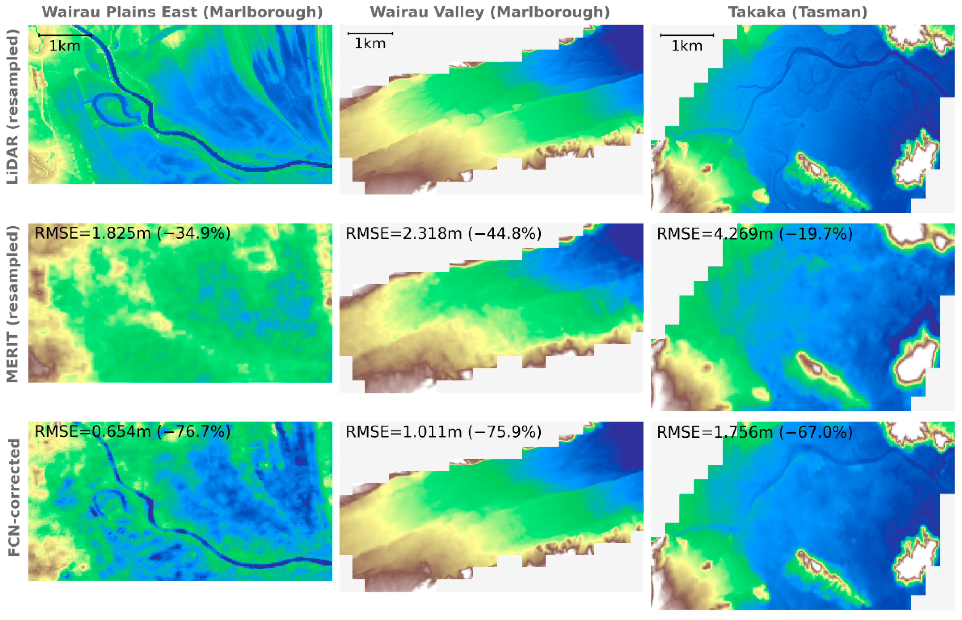
A more direct comparison is possible for the MERIT DEM developed by Yamazaki et al. [27], which involved the use of multiple filtering techniques to remove absolute bias, vegetation bias, speckle noise and stripe noise to produce an improved global DEM. The MERIT DEM has a horizontal resolution of 3 arc-seconds, so it was first resampled to match the resolution (1 arc-second) and alignment of the datasets used here, before calculating its vertical error in the testing zones (in terms of RMSE, with reference to the LiDAR-derived DTM). For these particular zones, while the MERIT DEM does represent an improvement over the original SRTM (reducing RMSE by 29%), all of the models explored here were able to achieve significantly higher improvements (ranging from 55% for the RF model to 71% for the FCN model).
Figure 21 compares the resampled LiDAR DTM with the resampled MERIT DEM and the FCN-corrected SRTM, across all three test zones, with labels showing the associated RMSE (judged against the resampled LiDAR DTM) and how this compares with that of the raw SRTM data (as a percentage reduction). At least in these particular locations, the FCN corrections are found to match the LiDAR DTM much more closely than the MERIT DEM, especially in terms of resolving river channels by stripping away the thick vegetation bias that frequently obscures them.

Figure 21.
A comparison of topography data across the three test sites, showing the reference LiDAR DTM (first row), the resampled MERIT DEM [27] (second row), and the FCN-corrected SRTM (third row), with labels indicating the RMSE and improvement over raw SRTM for each.
6. Conclusions
The research presented here suggests that machine learning models have real potential for correcting the vegetation and building biases known to affect free global DEMs such as SRTM. Given the number of large-scale flood hazard assessments which continue to rely on these free DEMs, being able to apply meaningful corrections could have significant downstream value for the flood maps produced, risk metrics calculated, and adaptation/mitigation recommendations made.
We investigated three different machine learning models, a relatively simple model (random forest), a densely-connected neural network (as has been used to address this task in the most recent research efforts) and a fully-convolutional neural network (a type of neural network developed specifically for image processing tasks). Given the spatial nature of the task at hand, it is perhaps no surprise that this latter model was found to perform best (on both the validation and test data), most likely as a result of its capacity to learn from spatial patterns at a variety of different scales. Over three test sites (i.e., data unseen during previous steps), the predicted corrections reduced the overall RMSE by 71% and were found to be especially effective at resolving river channels (which were often obscured in the original SRTM by thick vegetation along the banks).
Our results also suggest that models are likely to be biased towards the particular relationships/patterns most prevalent in the training data provided to them, raising questions about the importance of training models on input data which are as representative as possible of the intended application area(s). To inform the effective future application of the methods presented here, further work is required to assess just how important this is, balanced against the reduction in training dataset size which such pre-filtering would result in.
In terms of future developments of the research shared here, gradual increases in the spatial resolution of remote-sensed imagery suggest that a natural next step would be to increase the horizontal resolution of the input DEM at the same time as predicting its vertical biases (similar to the use of panchromatic satellite imagery to “pansharpen” other, coarser spectral band imagery [64]). If successful, such increases in horizontal resolution–coupled with effective vertical bias reduction–could allow for significant improvements in large-scale flood hazard mapping and assessment.
Supplementary Materials
The following are available online at https://www.mdpi.com/2072-4292/13/2/275/s1: Figure S1: Results of the sequential forward floating selection (SFFS) process used to select the most important input features (23) from all available (26); Table S1: All input features considered (66), indicating those selected for use in the modelling (23); Table S2: Summary of the RF hyperparameter values used; Table S3: Summary of the DCN hyperparameter values used; Table S4: Summary of the FCN hyperparameter values used; Section S1: Feature selection; Section S2: Model implementation. All of the Python code used to process data, build and train models, and visualise results is available online at https://github.com/mdmeadows/DSM-to-DTM.
Author Contributions
Conceptualisation, M.M. and M.W.; methodology, M.M. and M.W.; software, M.M.; validation, M.M. and M.W.; formal analysis, M.M.; investigation, M.M.; resources, M.W.; data curation, M.M.; writing—original draft preparation, M.M.; writing—review and editing, M.W.; visualisation, M.M.; supervision, M.W.; project administration, M.W. All authors have read and agreed to the published version of the manuscript.
Funding
This research received no external funding.
Institutional Review Board Statement
Not applicable.
Informed Consent Statement
Not applicable.
Data Availability Statement
The data presented in this study are openly available from a range of different data portals and online repositories, with access links provided in Section S1 (Supplementary Materials).
Acknowledgments
Thank you to the staff in Location Information at LINZ for their assistance in vertical datum transformations between the NZVD2016 and EGM96 geoid models, to Ryan Paulik (NIWA) for sharing the flood hazard maps that informed our study site selection, to Anthony Milton for advice regarding convolutional neural networks, to Aning Kuswinarni for the sketch illustrating the difference between a DTM and a DSM, and to three anonymous peer reviewers for their helpful feedback. M. Meadows completed this research as part of the requirements for a Master of Disaster Risk and Resilience at the University of Canterbury, New Zealand. The support of Thomas Wilson and John Southward at the University of Canterbury, including the provision of computing resources, is gratefully acknowledged.
Conflicts of Interest
The authors declare no conflict of interest.
References
- UNDRR. Global Assessment Report on Disaster Risk Reduction; United Nations Office for Disaster Risk Reduction (UNDRR): Geneva, Switzerland, 2019. [Google Scholar]
- Data-Pop Alliance. Big Data for Climate Change and Disaster Resilience: Realising the Benefits for Developing Countries. Data-Pop Alliance of the Harvard Humanitarian Initiative (HHI), MIT Media Lab, and Overseas Development Institute (ODI): 2015. Available online: https://datapopalliance.org/item/dfid-big-data-for-resilience-synthesis-report/ (accessed on 1 December 2020).
- CRED. Economic Losses, Poverty & Disasters: 1998–2017; Centre for Research on the Epidemiology of Disasters (CRED): Brussels, Belgium, 2018. [Google Scholar]
- Simpson, A.L.; Balog, S.; Moller, D.K.; Strauss, B.H.; Saito, K. An urgent case for higher resolution digital elevation models in the world’s poorest and most vulnerable countries. Front. Earth Sci. 2015, 3, 50. [Google Scholar] [CrossRef]
- Kulp, S.A.; Strauss, B.H. CoastalDEM: A global coastal digital elevation model improved from SRTM using a neural network. Remote Sens. Environ. 2018, 206, 231–239. [Google Scholar] [CrossRef]
- O’Loughlin, F.E.; Paiva, R.C.D.; Durand, M.; Alsdorf, D.E.; Bates, P.D. A multi-sensor approach towards a global vegetation corrected SRTM DEM product. Remote Sens. Environ. 2016, 182, 49–59. [Google Scholar] [CrossRef]
- Jena, P.P.; Panigrahi, B.; Chatterjee, C. Assessment of Cartosat-1 DEM for Modeling Floods in Data Scarce Regions. Water Resour. Manag. 2016, 30, 1293–1309. [Google Scholar] [CrossRef]
- Hawker, L.; Bates, P.; Neal, J.; Rougier, J. Perspectives on Digital Elevation Model (DEM) Simulation for Flood Modeling in the Absence of a High-Accuracy Open Access Global DEM. Front. Earth Sci. 2018, 6, 233. [Google Scholar] [CrossRef]
- Sanders, B.F. Evaluation of on-line DEMs for flood inundation modeling. Adv. Water Resour. 2007, 30, 1831–1843. [Google Scholar] [CrossRef]
- Wilson, M.D.; Bates, P.; Alsdorf, D.; Forsberg, B.; Horritt, M.; Melack, J.; Frappart, F.; Famiglietti, J. Modeling large-scale inundation of Amazonian seasonally flooded wetlands. Geophys. Res. Lett. 2007, 34, 4–9. [Google Scholar] [CrossRef]
- Yan, K.; Di Baldassarre, G.; Solomatine, D.P. Exploring the potential of SRTM topographic data for flood inundation modelling under uncertainty. J. Hydroinform. 2013, 15, 849–861. [Google Scholar] [CrossRef]
- Domeneghetti, A. On the use of SRTM and altimetry data for flood modeling in data-sparse regions. Water Resour. Res. 2016, 52, 2901–2918. [Google Scholar] [CrossRef]
- Farr, T.G.; Rosen, P.; Caro, E.; Crippen, R.; Duren, R.; Hensley, S.; Kobrick, M.; Paller, M.; Rodriguez, E.; Roth, L.; et al. The Shuttle Radar Topography Mission. Rev. Geophys. 2007, 45, 33. [Google Scholar] [CrossRef]
- Boulton, S.J.; Stokes, M. Which DEM is best for analyzing fluvial landscape development in mountainous terrains? Geomorphology 2018, 310, 168–187. [Google Scholar] [CrossRef]
- Tachikawa, T.; Kaku, M.; Iwasaki, A.; Gesch, D.; Oimoen, M.; Zhang, Z.; Danielson, J.; Krieger, T.; Curtis, B.; Haase, J.; et al. ASTER Global Digital Elevation Model Version 2—Summary of Validation Results; National Aeronautics and Space Administration (NASA): Pasadena, CA, USA, 2011.
- NASA NASA and METI Release ASTER Global DEM Version 3. Available online: https://lpdaac.usgs.gov/news/nasa-and-meti-release-aster-global-dem-version-3/ (accessed on 9 August 2019).
- Takaku, J.; Tadono, T.; Tsutsui, K.; Ichikawa, M. Validation of “AW3D” Global DSM Generated from ALOS PRISM. ISPRS Ann. Photogramm. Remote Sens. Spat. Inf. Sci. 2016, 3, 25–31. [Google Scholar] [CrossRef]
- Yamazaki, D.; Baugh, C.A.; Bates, P.D.; Kanae, S.; Alsdorf, D.E.; Oki, T. Adjustment of a spaceborne DEM for use in floodplain hydrodynamic modeling. J. Hydrol. 2012, 436–437, 81–91. [Google Scholar] [CrossRef]
- Becek, K. Assessing global digital elevation models using the runway method: The advanced spaceborne thermal emission and reflection radiometer versus the shuttle radar topography mission case. IEEE Trans. Geosci. Remote Sens. 2014, 52, 4823–4831. [Google Scholar] [CrossRef]
- Kulp, S.; Strauss, B.H. Global DEM Errors Underpredict Coastal Vulnerability to Sea Level Rise and Flooding. Front. Earth Sci. 2016, 4, 36. [Google Scholar] [CrossRef]
- Wendi, D.; Liong, S.-Y.; Sun, Y.; Doan, C.D. An innovative approach to improve SRTM DEM using multispectral imagery and artificial neural network. J. Adv. Model. Earth Syst. 2016, 8, 691–702. [Google Scholar] [CrossRef]
- Maire, C.; Datcu, M.; Audenino, P. SAR DEM filtering by mean of Bayesian and multi-scale, nonstationary methods. In Proceedings of the IGARSS 2003—2003 IEEE International Geoscience and Remote Sensing Symposium, Toulouse, France, 21–25 July 2003; Volume 6, pp. 3916–3918. [Google Scholar]
- Falorni, G.; Teles, V.; Vivoni, E.R.; Bras, R.L.; Amaratunga, K.S. Analysis and characterization of the vertical accuracy of digital elevation models from the Shuttle Radar Topography Mission. J. Geophys. Res. Earth Surf. 2005, 110, 1–20. [Google Scholar] [CrossRef]
- Stevenson, J.A.; Sun, X.; Mitchell, N.C. Despeckling SRTM and other topographic data with a denoising algorithm. Geomorphology 2010, 114, 238–252. [Google Scholar] [CrossRef]
- Ettritch, G.; Hardy, A.; Bojang, L.; Cross, D.; Bunting, P.; Brewer, P. Enhancing digital elevation models for hydraulic modelling using flood frequency detection. Remote Sens. Environ. 2018, 217, 506–522. [Google Scholar] [CrossRef]
- Zhao, X.; Su, Y.; Hu, T.; Chen, L.; Gao, S.; Wang, R.; Jin, S.; Guo, Q. A global corrected SRTM DEM product for vegetated areas. Remote Sens. Lett. 2018, 9, 393–402. [Google Scholar] [CrossRef]
- Yamazaki, D.; Ikeshima, D.; Tawatari, R.; Yamaguchi, T.; O’Loughlin, F.; Neal, J.C.; Sampson, C.C.; Kanae, S.; Bates, P.D. A high-accuracy map of global terrain elevations. Geophys. Res. Lett. 2017, 44, 5844–5853. [Google Scholar] [CrossRef]
- Saunders, W. Preparation of DEMs for use in environmental modeling analysis. In Proceedings of the ESRI User Conference, San Diego, CA, USA, 24–30 July 1999. [Google Scholar]
- Lary, D.J.; Zewdie, G.K.; Liu, X.; Wu, D.; Levetin, E.; Allee, R.J.; Malakar, N.; Walker, A.; Mussa, H.; Mannino, A.; et al. Machine Learning Applications for Earth Observation. In Earth Observation Open Science and Innovation; Mathieu, P., Aubrecht, C., Eds.; ISSI Scientific Report Series 15; International Space Science Institute (ISSI): Bern, Switzerland, 2018; ISBN 9783319656328. [Google Scholar]
- GFDRR. Machine Learning for Disaster Risk Management; Global Facility for Disaster Risk Reduction and Recovery (GFDRR): Washington, DC, USA, 2018. [Google Scholar]
- Yu, M.; Yang, C.; Li, Y. Big Data in Natural Disaster Management: A Review. Geosciences 2018, 8, 165. [Google Scholar] [CrossRef]
- Pyo, J.C.; Duan, H.; Baek, S.; Kim, M.S.; Jeon, T.; Kwon, Y.S.; Lee, H.; Cho, K.H. A convolutional neural network regression for quantifying cyanobacteria using hyperspectral imagery. Remote Sens. Environ. 2019, 233, 111350. [Google Scholar] [CrossRef]
- Parente, L.; Taquary, E.; Silva, A.P.; Souza, C.; Ferreira, L. Next generation mapping: Combining deep learning, cloud computing, and big remote sensing data. Remote Sens. 2019, 11, 2881. [Google Scholar] [CrossRef]
- Xie, B.; Zhang, H.K.; Xue, J. Deep convolutional neural network for mapping smallholder agriculture using high spatial resolution satellite image. Sensors 2019, 19, 2398. [Google Scholar] [CrossRef] [PubMed]
- Flood, N.; Watson, F.; Collett, L. Using a U-net convolutional neural network to map woody vegetation extent from high resolution satellite imagery across Queensland, Australia. Int. J. Appl. Earth Obs. Geoinf. 2019, 82, 101897. [Google Scholar] [CrossRef]
- Ronneberger, O.; Fischer, P.; Brox, T. U-net: Convolutional networks for biomedical image segmentation. Lect. Notes Comput. Sci. 2015, 9351, 234–241. [Google Scholar]
- Long, J.; Shelhamer, E.; Darrell, T. Fully Convolutional Networks for Semantic Segmentation. IEEE Trans. Pattern Anal. Mach. Intell. 2017, 39, 640–651. [Google Scholar]
- Jasanoff, S. Virtual, visible, and actionable: Data assemblages and the sightlines of justice. Big Data Soc. 2017, 4. [Google Scholar] [CrossRef]
- NIWA. New Zealand Fluvial and Pluvial Flood Exposure; National Institute of Water and Atmospheric Research (NIWA): Wellington, New Zealand, 2019. [Google Scholar]
- AAM NZ. Tasman District Council, Tasman DC LiDAR 2016-17, Volume 11327B01NOK; AAM NZ Limited: Napier, New Zealand, 2017. [Google Scholar]
- AAM NZ. Tasman District Council, Tasman DC LiDAR 2017-18, Volume PRJ30975NOB01; AAM NZ Limited: Napier, New Zealand, 2018. [Google Scholar]
- AAM NZ. Marlborough District Council, Marlborough DC LiDAR 2018, Volume PRJ31392NOM02; AAM NZ Limited: Napier, New Zealand, 2018. [Google Scholar]
- AAM NZ. Marlborough District Council, Marlborough DC LiDAR 2018, Volume PRJ31392NOM03; AAM NZ Limited: Napier, New Zealand, 2018. [Google Scholar]
- Wilson, M.F.; O’Connell, B.; Brown, C.; Guinan, J.C.; Grehan, A.J. Multiscale terrain analysis of multibeam bathymetry data for habitat mapping on the continental slope. Mar. Geod. 2007, 30, 3–35. [Google Scholar]
- ESA. S2 MPC, Level 2A Data Quality Report, Ref. S2-PDGS-MPC-L2ADQR; European Space Agency (ESA): Paris, France, 2020. [Google Scholar]
- Xu, H. Modification of normalised difference water index (NDWI) to enhance open water features in remotely sensed imagery. Int. J. Remote Sens. 2006, 27, 3025–3033. [Google Scholar] [CrossRef]
- Feyisa, G.L.; Meilby, H.; Fensholt, R.; Proud, S.R. Automated Water Extraction Index: A new technique for surface water mapping using Landsat imagery. Remote Sens. Environ. 2014, 140, 23–35. [Google Scholar] [CrossRef]
- Zha, Y.; Gao, J.; Ni, S. Use of normalized difference built-up index in automatically mapping urban areas from TM imagery. Int. J. Remote Sens. 2003, 24, 583–594. [Google Scholar] [CrossRef]
- Doll, C.N.H.; Muller, J.P.; Morley, J.G. Mapping regional economic activity from night-time light satellite imagery. Ecol. Econ. 2006, 57, 75–92. [Google Scholar] [CrossRef]
- Levin, N.; Duke, Y. High spatial resolution night-time light images for demographic and socio-economic studies. Remote Sens. Environ. 2012, 119, 1–10. [Google Scholar] [CrossRef]
- Mellander, C.; Lobo, J.; Stolarick, K.; Matheson, Z. Night-Time Light Data: A Good Proxy Measure for Economic Activity? PLoS ONE 2015, 10, e0139779. [Google Scholar] [CrossRef] [PubMed]
- Boeing, G. OSMnx: New methods for acquiring, constructing, analyzing, and visualizing complex street networks. Comput. Environ. Urban Syst. 2017, 65, 126–139. [Google Scholar] [CrossRef]
- Poppenga, S.K.; Worstell, B.B. Hydrologic Connectivity: Quantitative Assessments of Hydrologic-Enforced Drainage Structures in an Elevation Model. J. Coast. Res. 2016, 76, 90–106. [Google Scholar] [CrossRef]
- Lidberg, W.; Nilsson, M.; Lundmark, T.; Ågren, A.M. Evaluating preprocessing methods of digital elevation models for hydrological modelling. Hydrol. Process. 2017, 31, 4660–4668. [Google Scholar] [CrossRef]
- Simard, M.; Pinto, N.; Fisher, J.B.; Baccini, A. Mapping forest canopy height globally with spaceborne lidar. J. Geophys. Res. Biogeosci. 2011, 116, 1–12. [Google Scholar] [CrossRef]
- Hansen, M.C.; Potapov, P.V.; Moore, R.; Hancher, M.; Turubanova, S.A.; Tyukavina, A.; Thau, D.; Stehman, S.V.; Goetz, S.J.; Loveland, T.R.; et al. High-Resolution Global Maps of 21st-Century Forest Cover Change. Science 2013, 342, 850–854. [Google Scholar] [CrossRef] [PubMed]
- Pekel, J.F.; Cottam, A.; Gorelick, N.; Belward, A.S. High-resolution mapping of global surface water and its long-term changes. Nature 2016, 540, 418–422. [Google Scholar] [CrossRef]
- Akiba, T.; Sano, S.; Yanase, T.; Ohta, T.; Koyama, M. Optuna: A Next-Generation Hyperparameter Optimization Framework. In Proceedings of the ACM SIGKDD International Conference on Knowledge Discovery and Data Mining, Anchorage, AK, USA, 4–8 August 2019; pp. 2623–2631. [Google Scholar]
- Hastie, T.; Tibshirani, R.; Friedman, J. The Elements of Statistical Learning: Data Mining, Inference, and Prediction, 2nd ed.; Springer: Berlin/Heidelberg, Germany, 2017; ISBN 978-0-387-84857-0. [Google Scholar]
- Goodfellow, I.; Bengio, Y.; Courville, A. Deep Learning; MIT Press: Cambridge, MA, USA, 2016. [Google Scholar]
- Fukushima, K. Neocognitron: A hierarchical neural network capable of visual pattern recognition. Neural Netw. 1988, 1, 119–130. [Google Scholar] [CrossRef]
- LeCun, Y.; Boser, B.; Denker, J.S.; Henderson, D.; Howard, R.E.; Hubbard, W.; Jackel, L.D. Backpropagation applied to Handwritten Zip Code Recognition. Neural Comput. 1989, 1, 541–551. [Google Scholar] [CrossRef]
- Krizhevsky, A.; Sutskever, I.; Hinton, G.E. ImageNet Classification with Deep Convolutional Neural Networks. In Proceedings of the 25th International Conference on Neural Information Processing Systems, Tahoe NV, USA, 3–6 December 2012; Curran Associates Inc.: Red Hook, NY, USA, 2012; Volume 1, pp. 1097–1105. [Google Scholar]
- Yao, W.; Zeng, Z.; Lian, C.; Tang, H. Pixel-wise regression using U-Net and its application on pansharpening. Neurocomputing 2018, 312, 364–371. [Google Scholar] [CrossRef]
- Ma, L.; Liu, Y.; Zhang, X.; Ye, Y.; Yin, G.; Johnson, B.A. Deep learning in remote sensing applications: A meta-analysis and review. ISPRS J. Photogramm. Remote Sens. 2019, 152, 166–177. [Google Scholar] [CrossRef]
- Wieland, M.; Martinis, S. A modular processing chain for automated flood monitoring from multi-spectral satellite data. Remote Sens. 2019, 11, 2330. [Google Scholar] [CrossRef]
- Srivastava, N.; Hinton, G.; Krizhevsky, A.; Sutskever, I.; Salakhutdinov, R. Dropout: A Simple Way to Prevent Neural Networks from Overfitting. J. Mach. Learn. Res. 2014, 15, 1929–1958. [Google Scholar]
- Nobre, A.D.; Cuartas, L.A.; Hodnett, M.; Rennó, C.D.; Rodrigues, G.; Silveira, A.; Waterloo, M.; Saleska, S. Height Above the Nearest Drainage—A hydrologically relevant new terrain model. J. Hydrol. 2011, 404, 13–29. [Google Scholar] [CrossRef]
Publisher’s Note: MDPI stays neutral with regard to jurisdictional claims in published maps and institutional affiliations. |
© 2021 by the authors. Licensee MDPI, Basel, Switzerland. This article is an open access article distributed under the terms and conditions of the Creative Commons Attribution (CC BY) license (http://creativecommons.org/licenses/by/4.0/).


