Vegetation Abundance and Health Mapping Over Southwestern Antarctica Based on WorldView-2 Data and a Modified Spectral Mixture Analysis

Abstract

In polar regions, vegetation is especially sensitive to climate dynamics and thus can be used as an indicator of the global and regional environmental change. However, in Antarctica, there is very little information on vegetation distribution and growth status. To fill this gap, we evaluated the ability of both linear and nonlinear spectral mixture analysis (SMA) models, including a group of newly developed modified Nascimento’s models for Antarctic vegetated areas (MNM-AVs), in estimating the abundance of major Antarctic vegetation types, i.e., mosses and lichens. The study was conducted using WorldView-2 satellite data and field measurements over the Fildes Peninsula and its surroundings, which are representative vegetated areas in Antarctica. In MNM-AVs, we introduced secondary scattering components for vegetation and its background to account for the sparsity of vegetation cover and reassigned their coefficients. The new models achieved improved performances, among which MNM-AV3 achieved the lowest error for mosses (lichens) abundance estimation with RMSE = 0.202 (0.213). Compared with MNM-AVs, the linear model performed particularly poor for lichens (RMSE = 0.322), which is in contrast to the case of mosses (RMSE = 0.212), demonstrating that spectral signals of lichens are more prone to mix with their backgrounds. Abundance maps of mosses and lichens, as well as a map of moss health status for the entire study area, were then obtained based on MNM-AV3 with around 80% overall accuracy. Moss areas account for 0.7695 km² in Fildes and 0.3259 km² in Ardley Island; unhealthy mosses amounted to 40% (49%) of the area in the summer of 2018 (2019), indicating considerable environmental stress.

1. Introduction

The Antarctic ecosystem is particularly unique and fragile. Vascular plants are very rare, while mosses and lichens dominate and are distributed in small patches [1,2,3,4,5]. The Intergovernmental Panel on Climate Change (IPCC) 5th Assessment Report pointed out that dramatic changes in the climate system have been observed since the 1950s [6], and that they have severely affected the terrestrial biosphere in polar regions [7,8,9,10]. Climate change increased temperatures and water supplies in the ice-free areas of Antarctica, and vegetation has been responding quickly to adapt to these changes [11]. Due to the inconsistent warming over the Antarctic continent [12,13], vegetation has presented complex and heterogeneous responses, and the patterns have deeply concerned scientists [8,14,15]. Detailed information is needed, including the abundance, distribution, and health dynamics of typical vegetation types, to understand the rule of change and response mechanisms of Antarctic vegetation.

Vegetation mapping in Antarctica has been mainly based on field surveys [3,4,16,17,18,19]. However, field surveys are extremely time-consuming, greatly limiting information acquisition over large areas. Moreover, any human activity can cause permanent damage to slowly growing polar vegetation. Advances in remote sensing provide the opportunity to periodically and continuously observe Antarctic vegetation. Fretwell et al. [20] and Casanovas et al. [21,22] studied the distribution of Antarctic vegetation using the Normalized Difference Vegetation Index (NDVI) and the matched filtering (MF) approach derived from Landsat images, but the research were unable to identify a pattern between the NDVI values and the vegetation types. Sotille et al. [23] assessed the ability of the NDVI from unmanned aerial vehicle (UAV), Sentinel-2, and Landsat 8 to identify vegetated areas in the ice-free environment of Hope Bay, Antarctic Peninsula, and showed that the NDVI values provided by different sensors were not identical for the same vegetation class. More problematically, because polar vegetation clusters are usually very small [24], a pixel with a decameter spatial resolution usually includes a mix of plants, rocks, soil, and snow backgrounds, leading to poor classification results. Very high resolution (VHR) images such as IKONOS and QuickBird have been employed in the past to overcome this limitation [25,26]; however, because these images have only four bands, they cannot adequately discriminate between lichens and rocks. WorldView-2 (WV-2) imagery has eight bands that can capture most of the spectral characteristics of typical Antarctic vegetation, providing new mapping opportunities. Power [27] used WV-2 coupled with in situ surveying, imaging, and sampling to systematically estimate microbial mat biomass based on NDVI in Taylor Valley, Antarctica. UAV with hyperspectral sensor and higher spatial resolution was used to measure the reflectance spectroscopic characteristics of mats in McMurdo Dry Valleys to determine whether mats’ presence, types, and activities could be mapped at a spatial scale sufficient to characterize their interannual changes [28]. Relevant studies obtained vegetation distribution maps based on supervised classification methods including support vector machines [29], neural net classifiers [30], and spectral index ratios [31]. However, large training and verification datasets are difficult to collect in this region due to the harsh environmental conditions, severely limiting classification accuracy.

The aforementioned classification methods are referred to as “hard classifiers”, and assume that most pixels are pure [32]. In contrast, the “soft classifier” considers that most pixels are mixed and calculates the percentage of all the classes (i.e., abundance) for each pixel based on their spectral signatures [33,34]. This type of classifier does not require large training sets because it only needs to characterize the spectral signatures of potential categories, largely benefitting studies of Antarctic vegetation. These methods are usually referred as spectral mixture analysis (SMA) models. Shin et al. [3] generated the first vegetation abundance map over the Barton Peninsula of King George Island, Antarctica, using a linear SMA method based on QuickBird and KOMPSAT-2 images. Morison et al. [35] used spectroscopic methods and SMA to detect crustose lichen species and found that the relative reflection levels in different wavelengths can effectively discriminate lichens, particularly in the case of lichen–rock unmixing. Zhang et al. [36] estimated the abundance of five kinds of lichens using the spectral mixture analysis (SMA) method. Verified against field observations, Theau et al. [34] showed that SMA can characterize variations in lichens abundance and provides additional information compared with hard classifiers. To determine the most important spectral ranges for Antarctica vegetation discrimination, Calviño-Cancela et al. [37] adopted the linear discriminant analysis (LDA) method. This method was also applied in a similar environment of North Alaska based on field spectroscopy and multispectral satellite data to map dominant vegetation distributions [38]. Compared with Antarctica, Arctic regions possess more complicated vegetation types, and four tundra communities at Ivotuk, Alaska were discriminated based on their spectral information [39]. However, because plants in Antarctica are short and sparse (thus mixed with background such as rocks and soils), ignoring the scattering between vegetation and background endmembers limited the accuracy of these studies.

In addition to the distribution of Antarctic vegetation, variations in mosses growth and health status are also good indicators of climate change. Bartak et al. [40] used Global Positioning System instruments to measure moss-dominated vegetation areas located on James Ross Island, providing datasets for a long-term study of the biodiversity in Antarctica. Robinson et al. [41] used digital image analysis to estimate the percentage cover of mosses based on the leaf color, and monitored health and biodiversity in well-developed mosses communities in East Antarctica over 13 years (2000–2013). Changes in the relative abundance of mosses and their relationships with environmental parameters were analyzed. King et al. [42] proposed semi-automatic object-based image analysis (OBIA) to classify digital photographs with different moss health status using a set of rules based on information in red, green, and blue channels, as well as their hue-saturation-intensities (HSI), which have informed a conceptual framework for the changing condition of Antarctic mosses. Malenovskyet al. [43] explored the possibility of using near-distance imaging spectroscopy in the moss-bed health assessment, i.e., water-deficient (stressed) and well-watered (unstressed), and mentioned that the method could provide quantitative maps for Antarctic moss-bed health once applied to remotely-sensed hyperspectral images. These studies focused on digital photographs and UAV data, while few studies have addressed such monitoring based on satellite images. The probably most close study was conducted by Turner et al. [44], which developed several noninvasive spectroscopy-based methods to map the health state of moss beds near an Australian Antarctic station (Casey). The study identified an optimal UAV sensor capable of mapping a relatively large moss bed with the accuracy similar to that of the hyperspectral system, which provided a reference for similar studies using satellite images.

To facilitate the dynamic monitoring of Antarctic vegetation, this study evaluated the ability of VHR satellite images for vegetation abundance estimating and mosses health monitoring. We firstly explored the performance of both linear and nonlinear SMA models on mosses and lichens abundance mapping based on the WV-2 imagery. Results of linear and nonlinear models were compared against ground truth samples collected in the field survey over a typical vegetated area in Antarctica. A group of modified Nascimento’s models (MNM-AVs) were then proposed especially for Antarctic vegetated areas to modify the nonlinear coefficients by considering secondary scattering components between vegetation and backgrounds and improving the estimation accuracy. Finally, the best MNM-AV model was applied to generate abundance maps of mosses and lichens, as well as the moss heath status of the entire study area, based on WorldView-2 images. The model performance and the variation of moss heath status in two consecutive years were analyzed.

2. Study Area and Datasets

2.1. Study Area

Our study area (Figure 1) includes the Fildes Peninsula, Ardley Island and a part of the Nelson Peninsula (62°08′ S-62°14′S,58°40′S-59°02′S). The area is located southwest of King George Island, which is the closest island to the north end of the Antarctic Peninsula (AP) and has rich vegetation diversity [45,46,47]. Fildes Peninsula has 28.8 km² of ice-free area and Ardley has 1.2 km² [48]. The Great Wall Station of China is located on the Fildes Peninsula, and facilitated the collection of sufficient field measurements to support the study.

The region is within the sub-Antarctic maritime climate zone, where the weather is cold and windy, characterized by a mean annual temperature of –2 °C and wind speed of 7–8 m/s [39,49]. The land surface is covered by snow most of the year. The precipitation is abundant and evenly distributed throughout different seasons, with annual precipitation around 350–500 mm [39,50]. The topography of this area is characterized by two high structural volcanic platforms (Meseta Sul, 167 m, and Meseta Norte, 155 m), and in the other parts, the altitudes are mainly below 50 m [51]. The biota in this area is uniquely adapted to its special climate. The ecosystem is dominated by cryptogams, including mosses (mainly Sanionia sp., Andreaea sp., and Warnstorfia) and lichens (mainly Usnea Antarcti, Usnea aurantiacoatra, and Himantormia sp.), while vascular plants are very rare (only Deschampsia antarctic) [4,37,39,48,52]. The vegetation abundance is higher in existing or past animal (Pygoscelis adeliae penguin) habitats with rich organic soil [53]. The ecological environment of the region is very fragile and primitive, which makes it extremely sensitive to environmental stresses.

2.2. Remote Sensing Data

Vegetation information was extracted from WV-2 images acquired on 23 March 2018 and 19 February 2019. The dates corresponded to clear days in the austral summer growing season (January–March). WV-2 is a VHR satellite system with eight multi-spectral bands (

Table 1. Description of WV-2 multispectral bands.

Bands	Spectral Range (nm)	Characteristics
Band 1 Coastline	400–450	lichen absorption
Band 2 Blue	450–510	lichen reflection
Band 3 Green	510–580	moss health status
Band 4 Yellow	582–625	snow reflection
Band 5 Red	620–690	vegetation absorption
Band 6 RedEdge	705–745	moss health status
Band 7 NIR1	770–895	vegetation reflection
Band 8 NIR2	860–1040	vegetation reflection

), which provides us an opportunity to use high spatial and multispectral information at the same time. The system was launched on 6 October 2009, operating on a 770-km-high solar synchronous orbit supporting a 1.1-day revisit period. The resolution is 0.5 m for the panchromatic (PAN) waveband, and 2 m for the multispectral bands. The spectral bands 1, 2, 6, 7, and 8 are particularly useful for discriminating mosses and lichens from other land surface types.

2.3. Field Measurement Data

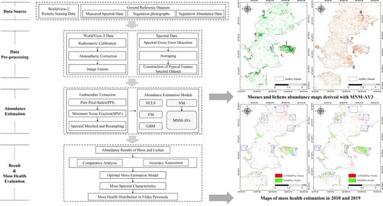
We carried out two field surveys, in February 2018 and February 2019, and collected vegetation abundance and spectral signatures in 32 typical vegetated sites across the study area (marked in Figure 1). We assumed that vegetation abundance remained unchanged in the two summers, considering that vegetation grows very slowly in Antarctica, while the mosses statuses changed rapidly. Each sampling site contained three to four sampling plots (2 m × 2 m), and the plots were chosen in relatively homogeneous areas distributed with typical vegetation types. Figure 2 shows example images of the plots.

For each plot, the spectral signatures of typical ground objects were measured using an SVR-HR1024 spectrometer. The spectrometer has a band range of 280–1094 nm with a 2 nm spectral resolution. We chose clear and cloudless times to continuously collect eight spectral signatures at each sampling point to ensure accuracy. The latitude and longitude of the measurement location, device height, vegetation type, abundance, and photographs were recorded at the same time. A total of 312 valid spectra signatures were collected, containing signatures of mosses in different health statuses, typical species of lichens (Usnea Antarctic and Usnea aurantiacoatra) and rocks (the major background information), along with photographs of 50 plots indicating mosses statuses (26 in 2018, and 24 in 2019), in total.

3. Methodology

The overall workflow of the study consisted of three stages: (1) data preprocessing, (2) mosses and lichens abundance estimation, and (3) validation and moss health evaluation (Figure 3). The details of each stage are described as follows.

3.1. Data Preprocessing

The preprocessing of WV-2 included radiometric calibration, atmospheric correction, and image fusion [54]. The radiometric calibration was implemented using the Environment for Visualizing Image software (ENVI, version 5.2) to convert digital numbers (DN) to at-sensor radiance. The at-sensor radiance was then corrected to eliminate atmospheric influence with the Fast Line-of-sight Atmospheric Analysis of Spectral Hypercubes (FLAASH) module to convert the top-of-atmosphere (TOA) reflectance to surface reflectance. Furthermore, to maximumly avoid mixing pixels in heterogeneous areas, we sharpened the multispectral bands with the PAN band to inject spatial details into the spectral bands (Figure 4). The Gram–Schmidt method was selected, which has been reported to be the state-of-the-art method for WV-2 data [31]. After atmospheric correction, the images accurately reflected the spectral reflectance of mosses, lichens, and other ground features, and the pan-sharpening enhanced image was able to highlight additional details, such as the scientific investigation station. Note that the spectral information can be slightly distorted during the process, which may cause errors in the spectral analysis. Therefore, the sharpened image was only used for visual interpretation and verification.

To process the field-measured spectral signatures, we first compared the repeated observations for each sample. When multiple measurements were performed on the same object, we assumed that the spectral curves should be similar. However, due to the shift of the instrument or the sudden change of light during the measurement, spectra can present obvious errors, which causes them to be significantly different from the other curves. These questionable curves were removed in the processing. Then, the remaining spectra were averaged for separate categories in each sample. Although the study area included multiple kinds of lichens with separable spectra, following the suggestion of Zhang [36], we only adopted one endmember because their spectra characters are similar enough. Examples of processed spectra are shown in Figure 5. The mosses spectra are similar to those of green vascular plants because chlorophyll pigments dominate the spectral response in the visible bands and absorb most of the energy at wavelengths around 0.45 (blue) and 0.65 (red). There is a small reflection peak around 0.54 um (green), whereas the reflection rises sharply near 0.76 um, forming the "red edge" (a typical phenomenon of healthy vegetation). Mosses in different health conditions have different spectral reflection characteristics, mainly in the near-infrared band. The near-infrared reflection decreases systematically with increasing stress (Figure 5a–c), and the location of the "red edge" moves to a shorter wavelength when the health improves. For lichens, the spectral characteristics are rather different [55]. There is a "U-shaped" reflectance signature located around 400 nm. The reflectance in the visible band is basically flat and significantly higher than that of mosses or other green vascular plants. The "red edge" also exists in lichens spectra, which means that lichens show two sudden changes in the reflectance profile. In contrast, rock has an obvious absorption around 0.35 um, and the reflectance climbs slowly in the visible and near-infrared bands, similar to the lichens spectra.

3.2. Endmember Extraction

Endmembers represent the spectral signatures of pure materials. Collecting endmembers is the first step in SMA. First, we used the minimum noise fraction (MNF) transformation [56] to obtain the principal component bands. All the eight transformed bands were retained because they all contained valuable information of ground objects (Figure A1). The pixel purity indexing (PPI) method was adopted to select the endmembers by rating the spectral purity of each pixel with a relative value. During processing, MNF images were repeatedly projected onto n-dimensional scatter plots [56], and pixels with high values were selected as candidates of endmembers. We then used an n-dimensional visualizer to delineate clustered scatters, and determined five endmembers, i.e., mosses, lichens, rock, water, and snow. The results (Figure 6) show that, although the WV-2 endmember spectra have fewer details compared with those measured with the SVR-HR1024 spectrometer, the main characteristics of different ground features are retained. The spectra measured in the field survey were better candidates for endmembers, as they were better targeted, and were resampled to match the WV-2 image spectra. However, because we lacked field measurements of water and snow, we adopted their endmembers derived with PPI.

3.3. Vegetation Abundance Estimation

We adopted five SMA models with different assumptions to estimate the abundance of mosses and lichens (

Table 2. Models used in the experiment.

Model	Type	Assumptions
Fully Constrained Least Square (FCLS)	Linear	Assumes no interaction between the objects
Nascimento’s Model (NM)	Nonlinear	Considers the secondary interactions between objects
Fan’s Model (FM)	Nonlinear	Assume that the secondary scattering effects of two endmembers in the pixel are directly related to their abundance
Generalized Bilinear Model (GBM)	Nonlinear	Considers the energy consumption in the transmission process by adding adjustment coefficient
Modified Nascimento’s Models for Antarctic Vegetated areas (MNM-AV) 1-3	Nonlinear	Redistributes the virtual abundance considering the actual situation in AP

). The classical models fully constrained least square (FCLS), Nascimento’s model (NM), Fan’s model (FM), and generalized bilinear model (GBM) were selected to test the performances of both linear and nonlinear SMA. Modified Nascimento’s models for Antarctic vegetated areas (MNM-AV) 1–3 are a group of modified nonlinear SMA models proposed in this study to consider the redistribution of secondary scattering components between vegetation and backgrounds.

3.3.1. The Linear Mixture Model

The Linear mixture model [57] assumes that the pixel DN is a linear synthesis of the reflectance of the objects included in its footprint on the ground, and there is no interaction between the objects. The mathematical model is as follows:

$$r={\displaystyle \sum }_{i=1}^P{\beta }_i{m}_i+n$$

(1)

$${\displaystyle \sum }_{i=1}^P{\beta }_i=1$$

(2)

$$0\le {\beta }_i\le 1$$

(3)

where $r$ represents a single pixel in the $L\times P$ dimension; $P$ is the number of endmembers; $L$ is the dimension of spectra (the number of observed bands); ${\beta }_i$ is the abundance vector containing the fractions of $ith$ endmember, which constitutes the $\beta$ abundance matrix in $k\times P$ dimensions; $m_i$ denotes the $ith$ endmember signature with a $L\times k$ matrix; $n$ stands for additive noise. Note that, to be physically meaningful, abundance fractions are subject to nonnegativity and constant sum constraints, from which the name fully constrained least square (FCLS) is derived, i.e., Equations (2) and (3) are abundance sum-to-one constraints (ASC) and abundance nonnegativity constraints (ANC). In this study, P = 5 and L = 8. The FCLS algorithm formulates the linear unmixing of images as a constrained optimization problem.

3.3.2. Nonlinear Mixture Models

In many situations involving multiple scattering effects, the linear mixture model, which only considers single scattering, is not a good approximation [58]. In these cases, a nonlinear mixture model may provide a better estimate. The general estimation equation is expressed as:

$$y=f\left(M,\beta \right)+N$$

(4)

where $M$ is a mixing matrix; $\beta$ is the abundance vector containing the fractions of each endmember;$N$ represents noise. The estimation result of FCLS was used as the initial input.

In our study area, because the types of ground objects are relatively simple, the scattering effect of three or more times should be weak, and therefore we only considered the secondary scattering. The bilinear model can calculate the secondary interactions between objects, and has different mathematical forms according to different nonlinear coefficients. Widely-used bilinear models include Nascimento’s model (NM) [58], Fan’s model (FM) [59], the generalized bilinear model (GBM) [60,61], and the polynomial post-nonlinear model (PPNM). Because our image has only eight bands, and excessive nonlinear coefficients will lead to high deviations in the estimation, we chose NM, FM, and GBM for this study.

(a)

Nascimento’s model (NM)

In NM, a mixed pixel can be expressed as

$$y={\displaystyle \sum }_{l=1}^P{\alpha }_l{m}_l+{\displaystyle \sum }_{i=1}^{P-1}{\displaystyle \sum }_{j=i+1}^P{\beta }_{i,j}{m}_i☉m_j+n$$

(5)

where ${\alpha }_l$ is the abundance vector containing the fractions of the $lth$ endmember;${\beta }_{i,j}$ is the interaction between $ith$ and $jth$ endmember, which is the adjustment coefficient of the nonlinear effect, also regarded as virtual abundance; $m_i☉m_j$ is the matrix of the $ith$ endmember vector times the $jth$ endmember vector, called the Hadamard product given as

$$m_i☉m_j=\left[\begin{array}{c}{m}_{1,i}\\ \begin{array}{c}{m}_{2,i}\\ ⋮\\ m_{L,i}\end{array}\end{array}\right]☉\left[\begin{array}{c}{m}_{1,j}\\ \begin{array}{c}{m}_{2,j}\\ ⋮\\ m_{L,j}\end{array}\end{array}\right]=\left[\begin{array}{c}{m}_{1,i}{m}_{1,j}\\ \begin{array}{c}{m}_{2,i}{m}_{2,j}\\ ⋮\\ m_{2,i}{m}_{L,j}\end{array}\end{array}\right]$$

(6)

The parameters must meet the following constraint conditions:

$${\displaystyle \sum }_{l=1}^P{\alpha }_l+{\displaystyle \sum }_{i=1}^{P-1}{\displaystyle \sum }_{j=i+1}^P{\beta }_{i,j}=1$$

(7)

$${\alpha }_l\ge 0, {\beta }_{i,j}\ge 0\left(i\ne j\right)$$

(8)

(b)

Fan’s model (FM)

Assuming that the secondary scattering effects of two endmembers in the pixel are directly related to their abundance, Fan proposed FM by adding the Hadamard product of two endmembers as a virtual endmember in LMM. The model is given as

$$y={\displaystyle \sum }_{l=1}^P{\alpha }_l{m}_l+{\displaystyle \sum }_{i=1}^{P-1}{\displaystyle \sum }_{j=i+1}^P{\alpha }_i{\alpha }_j{m}_i☉m_j+n$$

(9)

with

$$0\le {\alpha }_l\le 1, {\displaystyle \sum }_{l=1}^P{\alpha }_l=1$$

(10)

where ${\alpha }_i{\alpha }_j$ is a nonlinear coefficient formed by the product of the abundance of two different endmembers $m_i$ and $m_j$ respectively, which is regarded as the virtual abundance.

(c)

Generalized bilinear model (GBM)

Halimi [62] proposed an improved bilinear model by adding an adjustment parameter ${\beta }_{i,j}$ to the FM to consider the energy consumption in the transmission process. The model is given as

$$y={\displaystyle \sum }_{l=1}^P{\alpha }_l{m}_l+{\displaystyle \sum }_{i=1}^{P-1}{\displaystyle \sum }_{j=i+1}^P{\beta }_{i,j}{\alpha }_i{\alpha }_j{m}_i☉m_j+n$$

(11)

with

$$0\le {\alpha }_l\le 1,0\le {\beta }_{i,j}\le 1,{\displaystyle \sum }_{l=1}^P{\alpha }_l=1$$

(12)

where ${\beta }_{i,j}$ is the coefficient for adjusting the nonlinear effect. When ${\beta }_{i,j}$ = 1, GBM is converted to FM, and when ${\beta }_{i,j}$ = 0, GBM is converted to FCLS.

3.3.3. Modified Nascimento’s Models for Antarctic Vegetated Areas (MNM-AVs)

The SMA nonlinear traditional model was introduced for the first time in the estimation of vegetation abundance in Antarctica. The secondary scattering between endmembers can be regarded as a "virtual abundance” as it only has physical meaning at the spectral level [62]. Therefore, despite the fact that nonlinear models improve the modeling of mixed pixel spectra, its applicability for the estimation of ground cover is limited. That is, although the traditional nonlinear models can simulate the interaction between endmembers, sometimes they are still unable to provide accurate abundance estimates, especially for Antarctic vegetation that has very sparse distribution. For example, the “virtual abundance” that accounts for the relative strength of vegetation–rock interaction can, however, not be interpreted as an actual physical part of the ground signal. As a consequence, the method will result in a significant underestimation of the abundance of actual ground objects, owing to ASC (Equation (7)). At the same time, introducing water endmembers in traditional nonlinear models can lead to errors because except for a few low-lying regions (e.g., lakes and sea), the water abundance in the Fildes Peninsula should be 0 in real cases. Note that in FM and GBM, abundances of different objects are directly derived according to the estimated coefficients, while in NM, the abundances can share a portion of the “virtual abundance” based on flexible restrictions. Therefore, to better match the actual situation of the study area, a group of modified NM with new restrictions was proposed.

First, we assumed that if the water abundance exceeded half of a pixel, the abundance could be preserved. Else, it must have been a mistake, and the related virtual abundance (i.e., the secondary scattering between mosses (lichens) and their backgrounds) was reassigned to the other non-background classes (i.e., mosses and lichens) with a certain fraction following two alternative assumptions: (1) the two elements in the interaction term(s) contributed equally to the “virtual abundance”, i.e., each shared half of the “virtual abundance” (Equation (13)); (2) vegetation classes were the major source of secondary scattering, and therefore, the whole “virtual abundance” was assigned to mosses or lichens (Equation (14)).

$$\{\begin{array}{c}{f}_{moss}=(f_1+\frac{1}{2}{\displaystyle \sum }{f}_{1,j})/\left(f_1+f_{\mathrm{water}}+f_2+f_3+f_5\right),j=2,3,4,5\\ f_{lichen}=(f_2+\frac{1}{2}{\displaystyle \sum }{f}_{2,j})/\left(f_1+f_{\mathrm{water}}+f_2+f_3+f_5\right),j=1,3,4,5\end{array}$$

(13)

$$\{\begin{array}{c}{f}_{moss}=(f_1+{\displaystyle \sum }{f}_{1,j})/\left(f_1+f_{\mathrm{water}}+f_2+f_3+f_5\right),j=3,5\\ f_{lichen}=(f_2+{\displaystyle \sum }{f}_{2,j})/\left(f_1+f_{\mathrm{water}}+f_2+f_3+f_5\right),j=1,3,5\end{array}$$

(14)

where $f_{moss}$ and $f_{lichen}$ are the modified abundances of mosses and lichens; $f_{water}$ is the modified water abundance with errors;$f_1$, $f_2, f_3, f_4$and $f_5$ stand for the abundances of mosses, lichens, rock, water, and snow of the original nonlinear NM, sequentially. $f_{1,j}$ denotes the fractions of secondary scattering between mosses and the other endmembers. Similarly, $f_{2,j}$ denotes the secondary scattering between lichens and other endmembers.

Results are denoted as MNM-AV1, MNM-AV2, and MNM-AV3, representing only corrected water abundance and “virtual abundance” reassigned with assumptions (1) and (2), respectively.

3.4. Moss Health Evaluation

To survive in the harsh environment, mosses in Antarctica have various mechanisms to overcome stress, including the production of photoprotective pigments [63,64] which can change their colors. They change from green to red and then to brown and grayish-black once the components of different pigments inside their “leaves” are affected [57] (Figure 7). Therefore, their colors (reflectance optical properties) can be used to reflect the activity of their chloroplasts and health status. We thus defined green mosses as healthy mosses and mosses with the other colors as unhealthy mosses. The differences between their spectra can be observed in Figure 8, where healthy mosses show higher near-infrared reflectance and lower red reflectance than unhealthy mosses. To separate mosses clusters with different health statuses, endmembers of healthy and unhealthy mosses were added to the optimal abundance estimation model. We assumed that a pixel belonged to healthy (unhealthy) mosses when the abundance of healthy (unhealthy) mosses was greater than 50%. A distribution map of moss health status can thus be obtained.

4. Results

4.1. Estimation of Vegetation Abundance

Based on the extracted endmember spectra and least squares method, the results of FCLS, NM, FM, GBM, and MNM-AVs were obtained to get the abundance maps of mosses and lichens. In-situ data collected from 32 sampling sites with different mosses and lichens abundances ranging from 0 to 100% were used to evaluate the abundance estimation results. Particularly when a location had both mosses and lichens, the abundance of each type was estimated and validated. Please note that, because polar vegetation grows very slowly and will not change drastically in a short period of time [65], we did not separate the abundance information measured in 2018 and 2019. The root mean square errors (RMSEs) and R² of different models are compared in

Table 3. Assessment of mosses abundance estimates derived with different models.

Model	FCLS	NM	FM	GBM	MNM-AV1	MNM-AV2	MNM-AV3
R2	0.750	0.660	0.803	0.825	0.786	0.788	0.782
RMSE	0.212	0.403	0.243	0.231	0.250	0.215	0.202

and

Table 4. Assessment of lichens abundance estimates derived with different models.

Model	FCLS	NM	FM	GBM	MNM-AV1	MNM-AV2	MNM-AV3
R2	0.557	0.670	0.726	0.713	0.673	0.723	0.692
RMSE	0.322	0.374	0.282	0.272	0.306	0.237	0.212

, where R² is obtained by the linear regression characterizing the degree of fit and RMSE measures the error between abundance estimation and true abundance. Scatter plots of estimated abundance versus ground truth abundance for mosses and lichens are displayed in Figure A3 and Figure A4 for further details.

In estimating mosses abundance, NM performs the worst, with the lowest R² and the highest RMSE, which may result from the unreasonable inclusion of a “virtual abundance”. The other models show similar performances, among which GBM achieves the highest R² and MNM-AV3 achieves the lowest RMSE. For lichens, results are generally worse than those of mosses, demonstrating difficulties of estimating lichen abundance due to their severely mixed spectral information with their backgrounds, especially when only remote sensing images with a few multispectral channels are used. NM also performs the worst, indicating that NM must be improved for the unique conditions of Antarctic vegetation. In contrast, the modified NM models show good performances, with MNM-AV2 achieving the second-highest R² and MNM-AV3 achieving the lowest RMSE, which highlights the success of our modification strategy. The linear model FCLS performs particularly poorly for lichens, unlike in the case of mosses. This demonstrates that secondary scattering components are not obvious for mosses, while they are not neglectable for lichens, in the study area. This further indicates that lichens are more prone to be mixed with backgrounds, due to their growth characteristics, while mosses are not. Considering that the performance of these models is similar in R² except in the case of NM, we paid more attention to RMSEs, and selected MNM-AV3 as the best model for further applications.

The abundance estimation results of mosses and lichens obtained with MNM-AV3 are displayed in Figure 9, and those of the other models are shown in Figure A2. We can observe that mosses mainly grow in the eastern part of Ardley Island (region 1), along the coastal regions of the Nelson Peninsula (region 2), and over the coastal and lake shore regions in the Fildes Peninsula (region 3–5); lichens are mostly distributed over the southeast coastal and most elevated areas (region 7–9). The abundances of both vegetation types are higher on Ardley Island, compared with the Fildes Peninsula and Nelson Peninsula. Mosses tended to grow on humid land surfaces, such as in coastal regions and windward slopes, while lichens were distributed more widely. Mosses might be more sensitive to moisture, and lichens are more affected by temperature. Abandoned and active colonies of penguins, petrels, and many mammals occurred in coastal areas and transferred nutrients from the sea to inland, enhancing vegetation growth. Please note that the diversities in lichen spectral signatures due to their natural occurrence may cause the underestimation of lichen abundance considering that only one endmember was used, which means that the actual distribution of lichens can be wider.

4.2. Evaluation of Moss Health Status

The spectra of healthy and unhealthy mosses were included in MNM-AV3 to generate mosses health distribution maps based on two WV-2 images in 2018 and 2019, respectively (Figure 10). The cloud and snow areas were premasked in both images to facilitate the comparison. The mosses photos collected in 2018 and 2019 field surveys were used as ground truth data to validate the results (

Table 5. Confusion matrix of mosses health evaluation.

Class	Unhealthy (pixel)	Non-moss	Healthy (pixel)	Commission (%)	Omission (%)	Produced Accuracy (%)	User Accuracy (%)
Unhealthy	6	0	0	0.00	40	60	100
Non-moss	1	10	5	37.50	9.09	90.91	62.50
Healthy	3	1	24	14.28	17.24	82.76	85.72
Total	10	11	29	—	—	—	—
Overall Accuracy: 80.00%

), in which mosses are yellow and brown when stressed, and gray-black when moribund. The overall accuracy was verified to be 80%, which demonstrates the applicability of the new method for mosses health evaluation. This accuracy is reasonably good, considering the difficulty in defining the boundaries between different health categories for such sparse and thin mosses cover. In [42], moss health evaluation based on digital photographs achieved only a slightly higher accuracy, which was 84% with 26% commission rate for Windmill Island, East Antarctica. For mosses clusters with mixed health status, healthy mosses can reflect more sunlight and dominate the reflection character [42], and therefore tend to be classified as the heathy mosses. Generally, we can see from the maps that healthy mosses mainly grow near the seashore and the windward slope of Ardley Island, while mosses tend to grow under stress in inland areas. Please also note that because only 50 ground truth points were available (10 for unhealthy mosses, 29 for healthy mosses, and 11 for non-moss objects including lichens and backgrounds), this validation accuracy cannot be overstated. More field data are needed to conduct a thorough assessment, and we plan to arrange another field survey in the near future to support further analysis.

Overall, unhealthy mosses accounted for 40% in 2018 and 49% in 2019 over the study area, which demonstrates concerning environmental stress. From the two moss health maps, we can identify the major locations where moss health status changed from 2018 to 2019. However, we had troubles in registering the two VHR images with sufficient precision affected by complicated geographical distortions, especially when reference points are extremely difficult to collect in such an area. Instead, we identified several regions that displayed obvious changes (blue boxes in Figure 10) and analyzed them by visual interpretations. For example, in region 1–3, unhealthy mosses in 2018 had disappeared in 2019, which could be the result of mortality caused by severe environmental stress. In region 4–6, changes from healthy to unhealthy mosses can be noticed, which indicates unfavorable climate in 2019. In region 7 and 8, we can observe newly-emerged mosses but in unhealthy status, which are unlikely to happen in the real case. This can probably be explained by the inadequate accuracy of moss abundance mapping (also determines moss classification accuracy), which is only 78%, and that mistakes can be amplified when calculating the changes. The health status of mosses is highly dynamic and closely related to their water supply, which is mainly driven by the melt snow and ice in Antarctica. Lack of water can cause rapid death of mosses, while they can recover quickly through resprouting new shoots on moribund turf when the environmental condition becomes favorable [40].

4.3. Uncertainties and Limitations

From the results, we can infer that VHR images can capture the heterogeneity of Antarctic vegetation while also bringing difficulties in image registration, which require high resolution digital elevation models (DEMs) and ground controlling points to address the complicated and subtle distortions. Shadows caused by topography and remaining snow patches on the image are important sources of omissions in vegetation mapping. However, because the WV-2 imagery only has eight spectral bands, we did not detect shadows in the SMA. The varying shadows thus may lead to false change signals when comparing results from different observations. Moreover, considering that spectral signatures of lichens can be diverse based on their colors, using a single endmember for them in the SMA could result in underestimations of their abundance. The endmember spectra and threshold for healthy and unhealthy moss separation may need to be adjusted when applying this method to other Antarctic vegetated areas. Note also that the accuracies of SMA methods are highly dependent on the settings of sensor channels. Using images with more bands that can reflect key spectral characteristics of Antarctic landscapes can improve the abundance estimation results.

5. Discussions

In this study, we demonstrated the possibility of generating abundance maps for Antarctic mosses and lichens using VHR satellite images and SMA models. These maps can facilitate the monitoring of Antarctic vegetation changes in response to global and regional climate change. Methods based on satellite images can effectively reduce the reliance on field surveys and, therefore, prevent the human damage in Antarctica.

The mosses and lichens abundance maps obtained in this study were compared with the lichen cover maps interpolated from field survey measurements in 2006 [66] and a vegetation map classified using NDVI and GNDVI in [48], respectively. We observed high consistency despite our results showing high spatial heterogeneity due to the high-resolution data source. Quantitatively, the extracted moss area is 0.7695 km² in Fildes and 0.3259 km² in Ardley Island, which are slightly larger than those mentioned in [48] (0.6646 km² in Fildes and 0.3165 km² in Ardley Island). This is probably because our extraction includes unhealthy mosses which are not likely to be identified by conventional spectral indexes that measure vegetation greenness, such as NDVI. This difference may also be caused by the enhanced vegetation growth (i.e., a greener Antarctica) in recent years. Miranda et al. [67] found that the proportion of lichens (Usnea sp.) to mosses was about 3:1 in Meseta Norte and the extent along its gentle northern slope in Fildes Peninsula. This is basically consistent with our results where lichens were distributed more widely in Fildes Peninsula than mosses. Vegetation mapping in Barton Peninsula, which is close to Fildes Peninsula in Southwestern Antarctica, also demonstrated high vegetation abundance along the southeastern shore and low-to-medium abundance in inland areas [3], which matches the distribution characteristics derived in our study.

Generally, results of mosses estimation are better than those of lichens, which mainly lies in lichens’ high spatial heterogeneity and mixed spectra with their backgrounds (rocks and/or soils) [67]. This phenomenon was also found in results of FLCS and other nonlinear SMA models. From the difference of performances between linear and nonlinear models for mosses and lichens respectively, we can see that the secondary scattering components for mosses are not obvious, while they are non-neglectable for lichens. This is also one of the factors that cause conventional SMA models to underestimate the abundance of lichens (Figure A4). Another possible error in lichen estimation is the assumption followed by previous studies which assumes that only one lichen spectrum would be sufficient in Antarctic vegetation mapping [36]. Calviño-Cancela et al. [37] showed separable differences in lichen spectra of different species, and indicated that no common patterns for all lichens could be found. This would hinder or totally prevent the detection of some lichen species in detailed vegetation studies using merely one lichen endmember. Therefore, adding spectra of different lichen species may help to improve the accuracy in SMA based on hyperspectral images. However, when using multispectral data, this should be carefully considered to prevent problems when the number of endmembers exceeds the number of spectral channels. VHR satellite sensors with more optical spectral bands are required to solve this problem.

Monitoring changes of moss health with remote sensing data is quite challenging. Existing studies were mostly based on digital photos, spectrometer data, and UAV images [41,42,67,68]. Particularly, disappearances of mosses from 2013 to 2017 were observed in [67], which supports the trend of increased environmental stress concluded by our results. Detecting changes in moss health using multispectral satellite data is very hard, especially for large areas, not only because it requires high spectral separation accuracy with limited numbers of bands, but also because of the need for high-precision geographic matching for different images. In this study, we used a fixed abundance threshold of 0.5 to separate healthy and unhealthy mosses. This simple setting may cause sudden change of the health status when the abundance of each type only changes a little around 0.5 (e.g., 0.47 to 0.53). Furthermore, the fractions of different pigments in mosses can be related with their species, which may indicate that endmembers of healthy and unhealthy mosses need to be collected locally. In addition, a study demonstrated that reflectance spectroscopy values of mosses species are highly dependent on their moisture content, which can change very rapidly [69]. Therefore, moss health status maps obtained in this study have inherent limitations in quantifying changes of different years, and thus cannot be overstated. This demonstrates the requirement of new methods and technologies with respect to remotely-sensed vegetation health monitoring. Nevertheless, results in our study can help us rapidly identify potentially changed areas, and one can then evaluate them with digital photos or UAV equipment.

6. Conclusions

In this paper, we extracted vegetation information in the Fildes Peninsula, Ardley Island, and a part of the Nelson Peninsula, based on WV-2 images and seven SMA models (FCLS, NM, FM, GBM, and three MNM-AVs). The MNM-AV3 model we proposed especially for Antarctica achieved the best performance in abundance estimation of both mosses and lichens with RMSE = 0.202 and 0.212, respectively. The comparison of FCLS and nonlinear SMA models indicates that lichens are more prone to spectrally mix with backgrounds while mosses are not in the study area. The model was also applied to evaluate the mosses’ health status and achieved 80% overall accuracy, verified with in-situ measurements. Results demonstrate the applicability of using SMA and WV-2 imagery in detailed information acquisition of Antarctic vegetation, as well as the effectiveness of our modified SMA model in vegetation abundance estimation, which provides a useful baseline for large-scale and long-term vegetation monitoring in Antarctica.

References

1. Longton, R.E. Biology of Polar Bryophytes and Lichens; Cambridge University Press: Cambridge, UK, 1988; p. 391. [Google Scholar] [CrossRef]
2. Bokhorst, S.; Huiskes, A.; Convey, P.; Aerts, R. The effect of environmental change on vascular plant and cryptogam communities from the Falkland Islands and the Maritime Antarctic. BMC Ecol. 2007, 7, 15. [Google Scholar] [CrossRef] [PubMed] [Green Version]
3. Shin, J.-I.; Kim, H.-C.; Kim, S.-I.; Hong, S.G. Vegetation abundance on the Barton Peninsula, Antarctica: Estimation from high-resolution satellite images. Polar Biol. 2014, 37, 1579–1588. [Google Scholar] [CrossRef]
4. Kim, J.; Ahn, I.-Y.; Hong, S.G.; Andreev, M.; Lim, K.-M.; Oh, M.; Koh, Y.; Hur, J.-S. Lichen flora around the Korean Antarctic Scientific Station, King George Island. Antarct. J. Microbiol. 2006, 44, 480–491. [Google Scholar]
5. Lee, J.S.; Lee, H.K.; Hur, J.S.; Andreev, M.; Hong, S.G. Diversity of the lichenized fungi in King George Island, Antarctica, revealed by phylogenetic analysis of partial large subunit rDNA sequences. J. Microbiol. Biotechnol. 2008, 18, 1016–1023. [Google Scholar] [PubMed]
6. Shen, Y.P.; Wang, Y.G. Key findings and assessment results of IPCC WGI Fifth assessment report. J. Glaciol. Geocryol. 2013, 35, 1068–1076. [Google Scholar]
7. Bergstrom, D.M.; Turner, P.A.M.; Scott, J.; Copson, G.; Shaw, J. Restricted plant species on sub-Antarctic Macquarie and Heard Islands. Polar Biol. 2005, 29, 532–539. [Google Scholar] [CrossRef]
8. Convey, P. Antarctic terrestrial biodiversity in a changing world. Polar Biol. 2011, 34, 1629–1641. [Google Scholar] [CrossRef]
9. Sancho, L.G.; Pintado, A. Evidence of high annual growth rate for lichens in the maritime Antarctic. Polar Biol. 2004, 27, 312–319. [Google Scholar] [CrossRef]
10. Torres-Mellado, G.; Jana, R.; Casanova-Katny, M. Antarctic hairgrass expansion in the South Shetland archipelago and Antarctic Peninsula revisited. Polar Biol. 2011, 34, 1679. [Google Scholar] [CrossRef]
11. Green, T.A.; Sancho, L.G.; Pintado, A.; Schroeter, B. Functional and spatial pressures on terrestrial vegetation in Antarctica forced by global warming. Polar Biol. 2011, 34, 1643–1656. [Google Scholar] [CrossRef]
12. Doran, P.T.; Priscu, J.C.; Lyons, W.B.; Walsh, J.E.; Fountain, A.G.; McKnight, D.M.; Moorhead, D.L.; Virginia, R.A.; Wall, D.H.; Clow, G.D. Antarctic climate cooling and terrestrial ecosystem response. Nature 2002, 415, 517–520. [Google Scholar] [CrossRef] [PubMed]
13. Turner, J.; Barrand, N.E.; Bracegirdle, T.J.; Convey, P.; Hodgson, D.A.; Jarvis, M.; Jenkins, A.; Marshall, G.; Meredith, M.P.; Roscoe, H. Antarctic climate change and the environment: An update. Polar Rec. 2014, 50, 237–259. [Google Scholar] [CrossRef] [Green Version]
14. Cannone, N.; Dalle Fratte, M.; Convey, P.; Worland, M.R.; Guglielmin, M. Ecology of moss banks on Signy Island (maritime Antarctic). Bot. J. Linnean Soc. 2017, 184, 518–533. [Google Scholar] [CrossRef]
15. Robinson, S.A.; Wasley, J.; Tobin, A.K. Living on the edge–plants and global change in continental and maritime Antarctica. Glob. Chang. Biol. 2003, 9, 1681–1717. [Google Scholar] [CrossRef] [Green Version]
16. Furmańczyk, K.; Ochyra, R. Plant communities of the Admiralty Bay region (King George Island, South Shetland Islands, Antarctic) I. Jasnorzewski Gardens. Pol. Polar Res. 1982, 3, 25–39. [Google Scholar]
17. Poole, I.; Hunt, R.J.; Cantrill, D.J. A Fossil Wood Flora from King George Island: Ecological Implications for an Antarctic Eocene Vegetation. Ann. Bot. 2001, 88, 33–54. [Google Scholar] [CrossRef] [Green Version]
18. Kim, J.H.; Ahn, I.-Y.; Lee, K.S.; Chung, H.; Choi, H.-G. Vegetation of Barton Peninsula in the neighbourhood of King Sejong Station (King George Island, maritime Antarctic). Polar Biol. 2007, 30, 903–916. [Google Scholar] [CrossRef]
19. De, F.; Victoria, F.; Pereira, A.; Costa, D. Composition and distribution of moss formations in the ice-free areas adjoining the Arctowski region, Admiralty Bay, King George Island, Antarctica. Iheringia Ser. Bot. 2008, 64, 81–91. [Google Scholar]
20. Fretwell, P.T.; Convey, P.; Fleming, A.H.; Peat, H.J.; Hughes, K.A. Detecting and mapping vegetation distribution on the Antarctic Peninsula from remote sensing data. Polar Biol. 2011, 34, 273–281. [Google Scholar] [CrossRef]
21. Casanovas, P.; Black, M.; Fretwell, P.; Convey, P. Mapping lichen distribution on the Antarctic Peninsula using remote sensing, lichen spectra and photographic documentation by citizen scientists. Polar Res. 2015, 34, 25633. [Google Scholar] [CrossRef] [Green Version]
22. Casanovas, P.; Lynch, H.J.; Fagan, W.F.; Naveen, R. Understanding lichen diversity on the Antarctic Peninsula using parataxonomic units as a surrogate for species richness. Ecology 2013, 94, 2110. [Google Scholar] [CrossRef]
23. Sotille, M.E.; Bremer, U.F.; Vieira, G.; Velho, L.F.; Petsch, C.; Simões, J.C. Evaluation of UAV and satellite-derived NDVI to map maritime Antarctic vegetation. Appl. Geogr. 2020, 125, 102322. [Google Scholar] [CrossRef]
24. Raynolds, M.K.; Walker, D.A.; Maier, H.A. NDVI patterns and phytomass distribution in the circumpolar Arctic. Remote Sens. Environ. 2006, 102, 271–281. [Google Scholar] [CrossRef]
25. Kim, S.-H.; Hong, C.-H. Antarctic land-cover classification using IKONOS and Hyperion data at Terra Nova Bay. Int. J. Remote Sens. 2012, 33, 7151–7164. [Google Scholar] [CrossRef]
26. Vieira, G.; Mora, C.; Pina, P.; Schaefer, C.E.R. A proxy for snow cover and winter ground surface cooling: Mapping Usnea sp. communities using high resolution remote sensing imagery (Maritime Antarctica). Geomorphology 2014, 225, 69–75. [Google Scholar] [CrossRef]
27. Power, S.N.; Salvatore, M.R.; Sokol, E.R.; Stanish, L.F.; Barrett, J.E. Estimating microbial mat biomass in the McMurdo Dry Valleys, Antarctica using satellite imagery and ground surveys. Polar Biol. 2020, 43, 1753–1767. [Google Scholar] [CrossRef]
28. Levy, J.; Cary, S.C.; Joy, K.; Lee, C.K. Detection and community-level identification of microbial mats in the McMurdo Dry Valleys using drone-based hyperspectral reflectance imaging. Antarct. Sci. 2020, 32, 367–381. [Google Scholar] [CrossRef]
29. Jawak, S.D.; Luis, A.J.; Fretwell, P.T.; Convey, P.; Durairajan, U.A. Semiautomated Detection and Mapping of Vegetation Distribution in the Antarctic Environment Using Spatial-Spectral Characteristics of WorldView-2 Imagery. Remote Sens. 2019, 11, 1909. [Google Scholar] [CrossRef] [Green Version]
30. Jawak, S.D.; Udhayaraj, A.; Luis, A.J. Geospatial mapping of vegetation in the Antarctic environment using very high-resolution WorldView-2 imagery. In Proceedings of the Land Surface and Cryosphere Remote Sensing III, New Delhi, India, 5 May 2016. [Google Scholar]
31. Jawak, S.D.; Luis, A.J. A spectral index ratio-based Antarctic land-cover mapping using hyperspatial 8-band WorldView-2 imagery. Polar Sci. 2013, 7, 18–38. [Google Scholar] [CrossRef] [Green Version]
32. Wahba, G. Support vector machines, reproducing kernel Hilbert spaces and the randomized GACV. In Advances in Kernel Methods-Support Vector Learning; Schölkopf, B., Burges, C.J.C., Smola, A.J., Eds.; MIT: Cambridge, MA, USA, 1998; pp. 125–143. [Google Scholar]
33. Ichoku, C.; Karnieli, A. A review of mixture modeling techniques for sub-pixel land cover estimation. Remote Sens. Rev. 1996, 13, 161–186. [Google Scholar] [CrossRef]
34. Théau, J.; Peddle, D.R.; Duguay, C.R. Mapping lichen in a caribou habitat of Northern Quebec, Canada, using an enhancement_classification method and spectral mixture analysis. Remote Sens. Environ. 2005, 94, 232–243. [Google Scholar] [CrossRef]
35. Morison, M.; Cloutis, E.; Mann, P. Spectral unmixing of multiple lichen species and underlying substrate. Int. J. Remote Sens. 2014, 35, 478–492. [Google Scholar] [CrossRef]
36. Zhang, J.; Rivard, B.; Sánchez-Azofeifa, A. Spectral unmixing of normalized reflectance data for the deconvolution of lichen and rock mixtures. Remote Sens. Environ. 2005, 95, 57–66. [Google Scholar] [CrossRef]
37. Calviño-Cancela, M.; Martín-Herrero, J. Spectral Discrimination of Vegetation Classes in Ice-Free Areas of Antarctica. Remote Sens. 2016, 8, 856. [Google Scholar]
38. Davidson, S.J.; Santos, M.J.; Sloan, V.L.; Watts, J.D.; Phoenix, G.K.; Oechel, W.C.; Zona, D. Mapping Arctic Tundra Vegetation Communities Using Field Spectroscopy and Multispectral Satellite Data in North Alaska, USA. Remote Sens. 2016, 8, 978. [Google Scholar] [CrossRef] [Green Version]
39. Øvstedal, D.; Lewis Smith, R. Lichens of Antarctica and South Georgia: A Guide to Their Identification and Ecology; Cambridge University Press: Cambridge, UK, 2001. [Google Scholar]
40. Bartak, M.; Váczi, P.; Stachoň, Z.; Kubešová, S. Vegetation mapping of moss-dominated areas of northern part of James Ross Island (Antarctica) and a suggestion of protective measures. Czech Polar Rep. 2015, 5, 75–87. [Google Scholar] [CrossRef] [Green Version]
41. Robinson, S.A.; King, D.H.; Bramley-Alves, J.; Waterman, M.J.; Ashcroft, M.B.; Wasley, J.; Turnbull, J.D.; Miller, R.E.; Ryan-Colton, E.; Benny, T.; et al. Rapid change in East Antarctic terrestrial vegetation in response to regional drying. Nat. Clim. Chang. 2018, 8, 879–884. [Google Scholar] [CrossRef] [Green Version]
42. King, D.H.; Wasley, J.; Ashcroft, M.B.; Ryan-Colton, E.; Lucieer, A.; Chisholm, L.A.; Robinson, S.A. Semi-Automated Analysis of Digital Photographs for Monitoring East Antarctic Vegetation. Front Plant Sci. 2020, 11, 766. [Google Scholar] [CrossRef]
43. Malenovský, Z.; Turnbull, J.D.; Lucieer, A.; Robinson, S.A. Antarctic moss stress assessment based on chlorophyll content and leaf density retrieved from imaging spectroscopy data. New Phytol. 2015, 208, 608–624. [Google Scholar] [CrossRef] [Green Version]
44. Turner, D.J.; Malenovský, Z.; Lucieer, A.; Turnbull, J.D.; Robinson, S.A. Optimizing Spectral and Spatial Resolutions of Unmanned Aerial System Imaging Sensors for Monitoring Antarctic Vegetation. IEEE J. Stars 2019, 12, 3813–3825. [Google Scholar] [CrossRef]
45. Pressel, S. The illustrated moss flora of Antarctica. Ann. Bot. 2009, 104, vi–vii. [Google Scholar] [CrossRef] [Green Version]
46. Øvstedal, D.; Smith, R. Further additions to the lichen flora of Antarctica and South Georgia. Nova Hedwig. 2009, 88, 157–168. [Google Scholar] [CrossRef]
47. Olech, M. Plant Communities on King George Island. In Geoecology of Antarctic Ice-Free Coastal Landscapes; Beyer, L., Bölter, M., Eds.; Springer: Berlin/Heidelberg, Germany, 2002; Volume 154, pp. 215–231. [Google Scholar]
48. Andrade, A.M.D.; Michel, R.F.M.; Bremer, U.F.; Schaefer, C.E.G.R.; Simões, J.C. Relationship between solar radiation and surface distribution of vegetation in Fildes Peninsula and Ardley Island, Maritime Antarctica. Int. J. Remote Sens. 2018, 39, 2238–2254. [Google Scholar] [CrossRef]
49. Xiao, C.S.; Liu, D.L.; Zhou, P.J. The Study of Total Number of Bacteria and Fungi isolated from the Fildes Peninsula in Antarctic. Antarct. Res. 1994, 6, 67–72. [Google Scholar]
50. Shen, J.; Xu, R.M.; Zhou, G.F.; Wu, B.L.; Huang, F.P. Research on the structure and relationship of terrestrial, freshwater, intertidal and shallow sea ecosystems in Fildes Peninsula, Antarctic. Chin. J. Polar Res. 1999, 11, 23–35. [Google Scholar]
51. Pina, P.; Vieira, G.; Bandeira, L.; Mora, C. Accurate determination of surface reference data in digital photographs in ice-free surfaces of Maritime Antarctica. Sci. Total Environ. 2016, 573, 290–302. [Google Scholar] [CrossRef]
52. Lee, Y.I.; Lim, H.S.; Yoon, H.I. Geochemistry of soils of King George Island, South Shetland Islands, West Antarctica: Implications for pedogenesis in cold polar regions. Geochim. Cosmochim. Acta 2004, 68, 4319–4333. [Google Scholar] [CrossRef]
53. Michel, R.F.M.; Schaefer, C.E.G.R.; López-Martínez, J.; Simas, F.N.B.; Haus, N.W.; Serrano, E.; Bockheim, J.G. Soils and landforms from Fildes Peninsula and Ardley Island, Maritime Antarctica. Geomorphology 2014, 225, 76–86. [Google Scholar] [CrossRef]
54. Digital Globe. Radiometric Use of World View-2 Imagery. 2012. Available online: www.digitalglobe.com/downloads/Radiometric_Use_of_WorldView-2_Imagery.pdf (accessed on 11 May 2019).
55. Rees, W.G.; Tutubalina, O.V.; Golubeva, E.I. Reflectance spectra of subarctic lichens between 400 and 2400 nm. Remote Sens. Environ. 2004, 90, 281–292. [Google Scholar] [CrossRef]
56. Jensen, J.R. Introductory Digital Image Processing: A REMOTE Sensing Perspective, 3rd ed.; Pearson Prentice Hall: Upper Saddle River, NJ, USA, 2005; pp. 431–465. [Google Scholar]
57. Adams, J.B.; Smith, M.O.; Johnson, P.E. Spectral mixture modeling: A new analysis of rock and soil types at the Viking Lander 1 Site. J. Geophys. Res. Sol. Earth 1986, 91, 8098–8112. [Google Scholar] [CrossRef]
58. Nascimento, J.M.P.; Bioucas-Dias, J.M. Nonlinear mixture model for hyperspectral unmixing. In Proceedings of the Image and Signal Processing for Remote Sensing XV, Berlin, Germany, 28 September 2009; p. 74770I. [Google Scholar]
59. Fan, W.; Hu, B.; Miller, J.; Li, M. Comparative study between a new nonlinear model and common linear model for analysing laboratory simulated-forest hyperspectral data. Int. J. Remote Sens. 2009, 30, 2951–2962. [Google Scholar] [CrossRef]
60. Altmann, Y.; Dobigeon, N.; Tourneret, J. Bilinear models for nonlinear unmixing of hyperspectral images. In Proceedings of the 2011 3rd Workshop on Hyperspectral Image and Signal Processing: Evolution in Remote Sensing (WHISPERS), Lisbon, Portugal, 6–9 June 2011. [Google Scholar]
61. Halimi, A.; Altmann, Y.; Dobigeon, N.; Tourneret, J. Nonlinear Unmixing of Hyperspectral Images Using a Generalized Bilinear Model. IEEE Trans. Geosci. Remote Sens. 2011, 49, 4153–4162. [Google Scholar] [CrossRef] [Green Version]
62. Somers, B.; Cools, K.; Delalieux, S.; Stuckens, J.; Van der Zande, D.; Verstraeten, W.W.; Coppin, P. Nonlinear Hyperspectral Mixture Analysis for tree cover estimates in orchards. Remote Sens. Environ. 2009, 113, 1183–1193. [Google Scholar] [CrossRef]
63. Dunn, J.L.; Robinson, S.A. Ultraviolet B screening potential is higher in two cosmopolitan moss species than in a co-occurring Antarctic endemic moss: Implications of continuing ozone depletion. Global Chang. Biol. 2006, 12, 2282–2296. [Google Scholar] [CrossRef]
64. Waterman, M.J.; Bramley-Alves, J.; Miller, R.E.; Keller, P.A.; Robinson, S.A. Photoprotection enhanced by red cell wall pigments in three East Antarctic mosses. Biol. Res. 2018, 51, 49. [Google Scholar] [CrossRef]
65. Selkirk, P.M.; Skotnicki, M.L. Measurement of moss growth in continental Antarctica. Polar Biol. 2007, 30, 407–413. [Google Scholar] [CrossRef]
66. Pang, X.P.; Li, Y.H. Eco-environmental spatial characteristics of Fildes Peninsula based on TuPu models. Adv. Polar Sci. 2012, 23, 155–162. [Google Scholar] [CrossRef]
67. Miranda, V.; Pina, P.; Heleno, S.; Vieira, G.; Mora, C.; Schaefer, C.E. Monitoring recent changes of vegetation in Fildes Peninsula (King George Island, Antarctica) through satellite imagery guided by UAV surveys. Sci. Total Environ. 2020, 704, 135295. [Google Scholar] [CrossRef]
68. Lucieer, A.; Turner, D.; King, D.H.; Robinson, S.A. Using an Unmanned Aerial Vehicle (UAV) to capture micro-topography of Antarctic moss beds. Int. J. Appl. Earth Obs. 2014, 27, 53–62. [Google Scholar] [CrossRef] [Green Version]
69. May, J.L.; Parker, T.; Unger, S.; Oberbauer, S.F. Short term changes in moisture content drive strong changes in Normalized Difference Vegetation Index and gross primary productivity in four Arctic moss communities. Remote Sens. Environ. 2018, 212, 114–120. [Google Scholar] [CrossRef]
Figure 1. Study area and field measurement sites. The image is color-coded with red: band 8, green: band 4, and blue: band 1 of the WorldView-2 (WV-2) satellite image acquired on 23 March 2018.(a) King George Island (b) Fildes Peninsula, Ardley Island and a part of the Nelson Peninsula.
Remotesensing 13 00166 g001
Figure 2. Examples of vegetation plots. (a) Plots collected in 2018: (i)–(iv): mosses in different health statuses, (v)–(vi): mixed mosses and lichens, (vii)–(ix): lichens. (b) Plots collected in 2019: (i)–(vi): plots of abundance measurement for mosses and lichens.
Remotesensing 13 00166 g002
Figure 3. The overall workflow of the study.
Remotesensing 13 00166 g003
Figure 4. Preprocessing results of the Worldview-2 image coded with red: band 5, green: band 3, and blue: band 2 (true color). (a) Image after atmospheric correction; (b) enhanced image after pan-sharpening.
Remotesensing 13 00166 g004
Figure 5. Spectral profiles for typical ground features in the study area, including (a) healthy mosses, (b) stressed mosses, (c) moribund mosses, (d) lichens, and (e) rocks. Bold lines denote the averaged spectral signatures.
Remotesensing 13 00166 g005
Figure 6. Five endmembers collected in the study area.
Remotesensing 13 00166 g006
Figure 7. Photos of (a) healthy mosses, green, (b) stressed mosses, red-brown, and (c) moribund mosses, grey-black, indicating total loss of photosynthetic pigments.
Remotesensing 13 00166 g007
Figure 8. (a) Field-measured spectra and (b) endmember spectra for healthy and unhealthy mosses.
Remotesensing 13 00166 g008
Figure 9. Vegetation abundance maps derived with modified Nascimento’s model for Antarctic vegetated areas (MNM-AV)3 (the best model) for mosses and lichens in the left and right panel, respectively. Regions 1–5 highlight regions with a high abundance of mosses, and regions 6–9 are regions with a high abundance of lichens. The red box indicates the area of the zoom window.
Remotesensing 13 00166 g009
Figure 10. Maps of moss health estimation in 2018 (a) and 2019 (b). The blue boxes highlight representative areas for mosses showing changed growth status.
Remotesensing 13 00166 g010