Article

Deep Learning for Feature-Level Data Fusion: Higher Resolution Reconstruction of Historical Landsat Archive

1
Department of Land, Air and Water Resources, University of California, Davis, CA 95616-8627, USA
2
Department of Computer Science, University of California, Davis, CA 95616-8562, USA
*
Author to whom correspondence should be addressed.
Remote Sens. 2021, 13(2), 167; https://doi.org/10.3390/rs13020167
Submission received: 30 November 2020 / Revised: 29 December 2020 / Accepted: 1 January 2021 / Published: 6 January 2021
(This article belongs to the Section Remote Sensing Image Processing)

Abstract

:

Simple Summary

Existing freely available global land surface observations are limited by medium to coarse resolutions or short time spans. Here we developed a feature-level data fusion framework using a generative adversarial network (GAN), a deep learning technique, to leverage Landsat and Sentinel-2 observations during their over-lapping period from 2016 to 2019, and reconstruct 10 m Sentinel-2 like imagery from 30 m historical Landsat archives. Our tests with both simulated data and actual Landsat/Sentinel-2 acquisitions showed that the GAN-based super-resolution method could accurately reconstruct synthetic Landsat data at an effective resolution very close to that of the real Sentinel-2 observations. The promising results from our deep learning-based feature-level fusion method highlight the potential for reconstructing a 10 m Landsat series archive since 1984. It is expected to improve our capability of detecting and tracking finer scale land changes, identifying the drivers for and responses to global environmental changes.

Abstract

Long-term record of fine spatial resolution remote sensing datasets is critical for monitoring and understanding global environmental change, especially with regard to fine scale processes. However, existing freely available global land surface observations are limited by medium to coarse resolutions (e.g., 30 m Landsat) or short time spans (e.g., five years for 10 m Sentinel-2). Here we developed a feature-level data fusion framework using a generative adversarial network (GAN), a deep learning technique, to leverage the overlapping Landsat and Sentinel-2 observations during 2016–2019, and reconstruct 10 m Sentinel-2 like imagery from 30 m historical Landsat archives. Our tests with both simulated data and actual Landsat/Sentinel-2 imagery showed that the GAN-based fusion method could accurately reconstruct synthetic Landsat data at an effective resolution very close to that of the real Sentinel-2 observations. We applied the GAN-based model to two dynamic systems: (1) land over dynamics including phenology change, cropping rotation, and water inundation; and (2) human landscape changes such as airport construction, coastal expansion, and urbanization, via historical reconstruction of 10 m Landsat observations from 1985 to 2018. The resulting comparison further validated the robustness and efficiency of our proposed framework. Our pilot study demonstrated the promise of transforming 30 m historical Landsat data into a 10 m Sentinel-2-like archive with advanced data fusion. This will enhance Landsat and Sentinel-2 data science, facilitate higher resolution land cover and land use monitoring, and global change research.

Graphical Abstract

1. Introduction

Many land changes occur at fine spatial scales ranging from meter to ~10 m [1,2], and thus remote sensing data at higher spatial resolution are needed to effectively detect and monitor these changes across landscapes. In order to understand the drivers associated with global environmental change, repeated observations over a long time period are also critical. The U.S. Geological Survey (USGS) Landsat series of satellites provides the longest temporal record of space-borne surface observations at 30 m [3]. It has been widely used for documenting how the Earth’s terrestrial ecosystem has changed over the past four decades [4,5], driven by the growing pressure of booming population, human modification, and climate change [6,7,8]. However, due to the mixed pixel problem [9,10], the 30 m spatial resolution of Landsat data still limits its applications for accurate quantification of biophysical properties and processes, especially over heterogeneous landscapes. For example, it is challenging to take full advantage of Landsat mission continuity to detect canopy-level flowering phenology [11], differentiate crop species [12,13], extract urban functional blocks [14], and map wetland and watershed interfaces [15].
The Sentinel-2 mission, initiated by the European Commission (EC) and the European Space Agency (ESA) constellation, on the other hand, aims to provide systematic global acquisition of fine-resolution multispectral imagery [16]. With the full operation of two identical satellites, Sentinel 2A/B has been able to provide an unprecedented observation of global land surfaces at a spatial resolution of 10–60 m with a five day revisiting cycle [16]. Given the relative fine spatial and temporal resolutions and free access to the full data archive, Sentinel-2 data has been used by an increasing number of end users in various research and applications, such as urban [14], agriculture [12], and forestry [17]. However, Sentinel-2 systems have had a relatively short five-year data record so far since the first launch of Sentinel-2A in 2015, thereby limiting its capability for long-term terrestrial change applications.
To take advantage of the complementary information from multiple sensors with varying spatial, temporal, and spectral characteristics, data fusion techniques have attracted tremendous interest within the remote sensing community over the past decades [18,19,20]. Many studies, for example, have focused on the spectral and spatial fusion via “pan-sharpening” [10,21,22,23]. Their main purpose is to generate high-resolution imagery at multiple spectral bands, by combining the multispectral characteristics at coarser spatial resolution with the fine spatial details from high spatial resolution panchromatic imagery. However, the outputs from pan-sharpening may suffer from spectral distortions, limiting their use in the field of quantitative remote sensing.
Spatio-temporal fusion has also been developed and applied to generate synthetic data at fine spatial resolution and with high temporal frequency, by blending remote sensing observations from multi-sensors with various spatial and temporal characteristics [6,19,20,24,25,26,27]. Among them, the spatial and temporal adaptive reflectance fusion model (STARFM) [19] is one of the most popular algorithms; it uses the concurrent image pairs of 30 m Landsat and 250 m MODIS to build the spatial relationship and adjusts the temporal dynamics with more frequent coarse-resolution MODIS observations [18,25]. However, the STARFM-like algorithms rely on at least one prior or posterior pair of fine and coarse spatial resolution images (e.g., Landsat and MODIS) acquired on the same day. This requirement makes the STARFM-like framework not suitable for fusing Landsat and Sentinel-2 images that often revisit at different overpassing days [28]. The temporal interpolation framework of STARFM-like algorithms make assumptions of no significant land cover changes occurring during the interpolated period [18,19]. This may cause large uncertainties in reconstructing historical Landsat imagery for denser time stacks. A fill-and-fit approach was also developed for land surface time series using alternative similar pixels for spatial filling and a harmonic model to gap fill the time series, based on a single year or growing season of Landsat [29]. These approaches are mostly designed for pixel-level observation fusion to generate continuous time series of the highest resolution available for tracking land surface dynamics. The feature perception information, however, has not been fully incorporated into fusion.
Several studies have been focused on the fusion of Landsat and Sentinel-2 images. For example, the NASA Harmonized Landsat and Sentinel-2 project creates a temporally denser Landsat-like surface reflectance datasets, by resampling 10 m Sentinel-2A and 2B data acquired every five days to match the 30 m resolution of Landsat. Although many efforts are made to ensure radiometric consistency, including atmospheric correction, cloud and cloud-shadow masking, spatial co-registration and common gridding, bidirectional reflectance distribution function normalization and spectral bandpass adjustment [30], finer spatial details from Sentinel-2 are not fully used for the fusion [28,31]. To overcome this issue, Wang et al. [31] proposed an area-to-point regression kriging (ATPRK)-based method to generate 10 m Landsat-8 like images, by fusing available 10 m Sentinel-2 and Landsat 8 panchromatic (PAN) bands. This geo-statistical fusion algorithm relies on the input covariates derived from the corresponding Sentinel-2 imagery to enhance spatial details of each lower-resolution imagery. However, ATPRK involves complex semi-variogram modelling from a co-kriging matrix, which is computationally expensive for large-scale super-resolution processing [28].
One possible cost-effective solution is to leverage Landsat and Sentinel-2 observations during their overlapping period, to reconstruct 10 m Sentinel-2-like imagery from historical Landsat imagery at 30 m before 2015. It is based on a transfer learning strategy enabled with deep learning algorithms in computer vision [32,33,34], e.g., applying the relationship learned from Landsat and Sentinel-2 over the most recent temporal period to historical pre-2015 Landsat data, to regenerate synthetic 10 m Landsat archive over the past four decades.
Convolution neural network (CNN)-based super-resolution (SR) image reconstruction has proven to be a promising approach in closing inherent resolution gaps of imaging sensors [33,35,36,37]. Here, we categorize existing deep learning CNN SR methods into two classes based on their main purpose. One class aims at optimizing distortion measures such as peak signal-to-noise ratio (PSNR), structural similarity index measure (SSIM), and mean square error (MSE) to yield more accurate images, and we named this group as PSNR-oriented methods. In order to achieve better quantitative measures, major solutions in this category consider pixel-wise loss functions and increase the network complexity of CNNs. For example, Ledig et al. [34] proposed SRResNet with 16 residual units to optimize MSE. Lim et al. [38] developed an enhanced deep super-resolution network (EDSR) to significantly improve the single image super-resolution performance by removing the batch normalization layers in SRResNet and increasing the number of residual blocks to 23.
Another group of image SR studies attempts to produce more photo-realistic images by including an extra perceptual loss function; these are superior in perceptual quality, thereafter referred as perceptual-oriented methods. For example, Johnson et al. [39] proposed perception loss to enhance the perceptual quality by minimizing the error in feature space instead of pixel space. A generative adversarial network (GAN) was also developed for image SR by applying both perceptual loss and adversarial loss to generate realistic textures during SR and achieves state-of-the-art performance [34]. Pouliot et al. [36] applied both shallow and deep convolution neural networks (CNNs) in Landsat image super-resolution enhancement, trained using Sentinel-2, in three study sites representing boreal forest, tundra, and cropland/woodland environments. An extended super-resolution convolutional neural network (ESRCNN) was developed [28], and it was suggested that the proposed deep learning models outperformed the ATPRK-based algorithm using experimental tests in two local study areas of North China’s Hebei province. However, these CNN approaches still fall into the category of non-GAN-based models without adding the adversarial discriminator to better tune the neural network. A similar non-GAN-based CNN model was used to super-resolve the lower-resolution bands (20 m and 60 m) of Sentinel 2 to 10 m spatial resolution, over 60 representative Sentinel-2 scenes across the globe [40].
Despite the promising results of these pilot studies, the evaluation and application of deep learning-based approaches in remote sensing data fusion of Landsat and Sentinel-2 is still limited. Firstly, most of existing studies working on the super-resolution of Landsat and Sentinel-2 rely on non-GAN-based models without fully coupling perceptual loss and adversarial loss into the CNN framework. Secondly, the training and tuning of deep learning algorithms in remote sensing data fusion is complex and sensitive to both spatial and temporal domains. Moreover, the majority of available studies are limited to local scales and short-temporal periods. Lastly, a comprehensive comparison of different algorithms, including statistical interpolation, geo-statistical modelling, non-GAN-based, and GAN-based deep learning models to super-resolve Landsat imagery from 30 m to 10 m, is needed to provide insights for practical applications. To our knowledge, there have been limited efforts so far on reconstructing 10 m Sentinel-2-like imagery from the historical Landsat archive using the state-of-the-art non-GAN and GAN-based deep learning approaches across different spatial and temporal scales.
Addressing these challenges, we aim to implement a feature-level data fusion framework for remote sensing SR image reconstruction. Specifically, we first developed the GAN-based fusion framework to leverage Landsat and Sentinel-2 observations during their overlapping period from 2016 to 2019, for reconstructing 10 m Sentinel-2-like imagery from historical 30 m Landsat archive. We then provided a comprehensive comparison of GAN-based deep learning models with baseline methods including statistical interpolation, geo-statistical modelling, non-GAN-based, to better inform SR model performance. We further investigated the potential of the GAN-based model in dynamic systems over different spatial and temporal domains. Finally we demonstrated the promise of transforming 30 m historical Landsat data into a 10 m Sentinel-2-like archive with this advanced data fusion.

2. Materials and Methods

2.1. Theoretical Basis

The aim of our study was to reconstruct an SR resolved image ISR to the same spatial resolution as Sentinel-2 (IHR), from a low spatial resolution Landsat image ILR with a convolutional neural network (CNN). A non-GAN-based network (Section 2.1.1) and a GAN-based network (Section 2.1.2) were both used in this study for the purpose of comparing the performance of PSNR-oriented and perceptual-oriented deep learning methods in remote sensing image SR tasks.
As shown in Table S1, Landsat series (i.e., Landsat-5/7/8) have very close bandwidths to Sentinel-2A/B, particularly over blue, green, and red bands. This provided a theoretical basis of spectral comparability to build a band-over-band relationship between Landsat and Sentinel-2. For the experimental purpose in this study, we focused on using the true color composite of red–green–blue bands for both Landsat and Sentinel-2. The proposed methods below can be extended to other paired bands and high–low resolution image pairs as well.

2.1.1. Deep Convolutional Neural Networks

For a low spatial resolution image ILR with W columns, H rows, and C bands, it can be expressed by a tensor of size W × H × C . Its corresponding IHR and ISR have the size of r W × r H × C , where r represents a scaling factor. In the training process, ILR and IHR image pairs were used as the input of a feed-forward CNN network G θ parameterized by θ . We adopted the SRResNet architecture [34] in this work, with the only difference in removing batch normalization (BN) layers in the residual block, because removing BN layers will help reduce computation costs and increase the model generalization ability [38]. As shown in Figure 1, SRResNet comprises 16 identical residual blocks using ParametricReLU as the activation function and downscaling with 2 trained sub-pixel convolution layers.
The objective function is:
θ ^ = a r g m i n θ E n [ l M S E ( G θ ( I L R n ) ,   I H R n ) ] ,   n   =   1 ,   2 ,   ,   N
where I L R n and I H R n are corresponding low-high spatial resolution training image pairs, N is the total number of training image pairs, l M S E is the most widely used loss function for image SR, which calculates the pixel-level MSE between I H R n and the generated image I S R n .

2.1.2. Generative Adversarial Networks

Generative adversarial networks (GAN), proposed by Goodfellow et al. [41] in 2014, have shown great breakthroughs in training unsupervised machine learning models and have gained popularity in computer vision fields. It consists of two networks; a generator G and a discriminator D. G is trained to generate output that is close to the real data. D is a multilayer perception model defined to distinguish whether a sample is from the generator or real data, represented as a simple binary classifier that outputs a single scalar.
For a better gradient performance, E n [ log ( D ( G ( x n ) ) ) ] is usually used as the G’s loss function. E x ~ p d a t a ( x ) [ log ( D ( x ) ) ] + E x ~ p g ( x ) [ log ( 1 D ( G ( x ) ) ) ] is a common form of the D’s loss function. D and G are trained in conjunction to solve a two-player min–max problem. G tries to fool D into labeling its sample as real data by minimizing its loss function and generating sample approximating real data distribution. D tries to maximize the probability of assigning the correct label to sample both from generator’s distribution ( p g ) and from data distribution ( p d a t a ).
A GAN-based model was constructed by taking the non-GAN-based model (Section 2.1.1) as the generator ( G θ ) and trained with a discriminator (Figure 2). The architecture of the discriminator we used closely followed ESRGAN [42], which is a relativistic average discriminator that instead of estimating if a generated image is real or fake, it estimates the realistic score of a generated image relative to real image.

2.1.3. Loss Function

The total loss of the generator G θ is the weighted combination of adversarial loss and perceptual loss defined as
l o s s S R = l V G G 19 54 + w l G
where w is the weight set to be 10−3, and l G is the generator’s loss E n [ log ( D ( G ( x n ) ) ) ] . VGG loss, l V G G 19 54 is the perceptual loss, defined as the L2-norm distance between the feature representations (i.e., feature obtained by the 4th convolution before the 5th maxpooling layer within the pre-trained 19-layer VGG network) of a generated image ISR and the reference high spatial resolution image IHR.

2.2. Implementation

The scaling factor r between ISR and IHR was 3 in all experiments, to be consistent with the spatial resolution difference between Landsat and Sentinel-2 dataset. The minimum batch size was set to be 16. Following the SRGAN, training images were cropped into 96 × 96 patches for each minimum batch.
For the simulated data experiment and real data experiment (Section 3.1 and Section 3.2), the modified SRResNet networks (referred as non-GAN-based network hereafter) were trained through 1 million iterations with the MSE loss, a learning rate of 10−4, and decayed by a factor of 2 at 50 k, 100 k, 200 k, and 300 k iterations.
When training the GAN-based model, we employed the trained non-GAN-based network as initialization for the generator to obtain better results [34]. GAN-based networks were trained with 5 × 10⁵ iterations at a learning rate of 10−4 and decayed by a factor of 2 every 2 × 10⁵ iterations. For optimization, we used the Adam method [43] with β 1 = 0.9 , β 2 = 0.999 , and ε = 10 8 . The generator and discriminator were updated alternatively. We implemented these networks using Python 3.7.6 with the PyTorch 1.0.1 framework and trained them using NVIDIA 2080 Ti GPU.

2.3. Landsat and Sentinel-2 Datasets

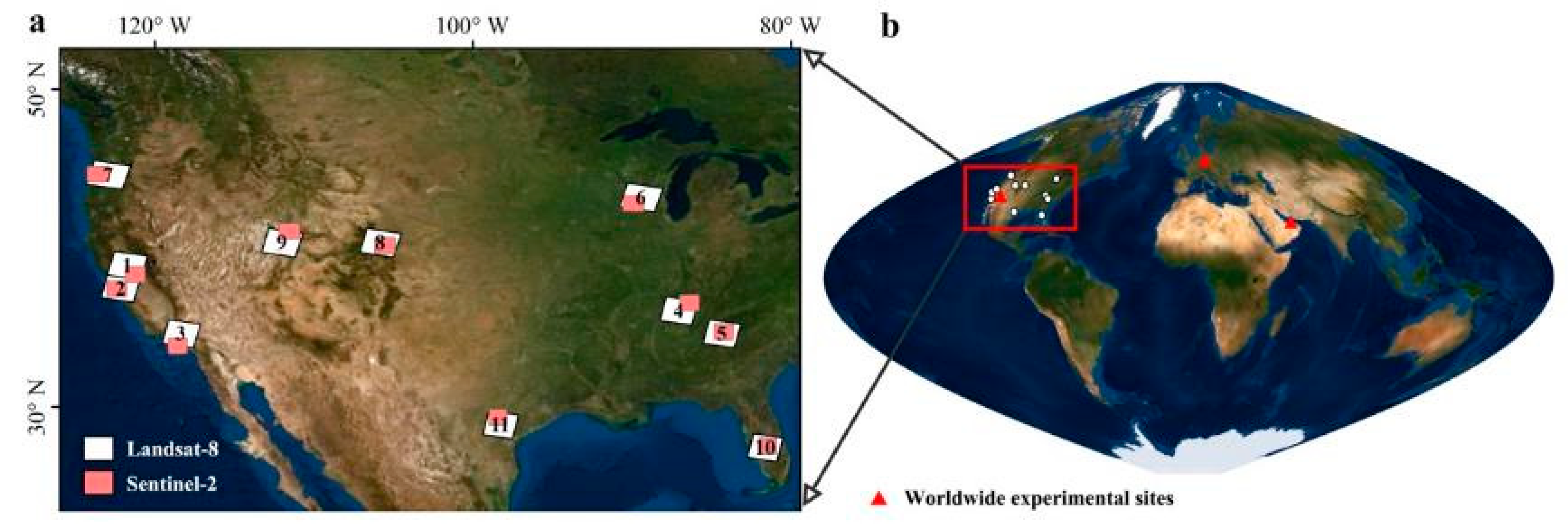
We selected study areas spatially distributed across different landscapes of the U.S., to provide more diverse terrestrial land cover information for training and testing (Figure 3a). A total of 11 cloud-free Landsat and Sentinel-2 imagery pairs from 2016 to 2019 were collected and downloaded from the Google Earth Engine (https://earthengine.google.com/) data archive (Table 1, Figure 3a). We identified Landsat and Sentinel-2 imagery pairs that both had less than 5% cloud cover and were less than 5 days apart.
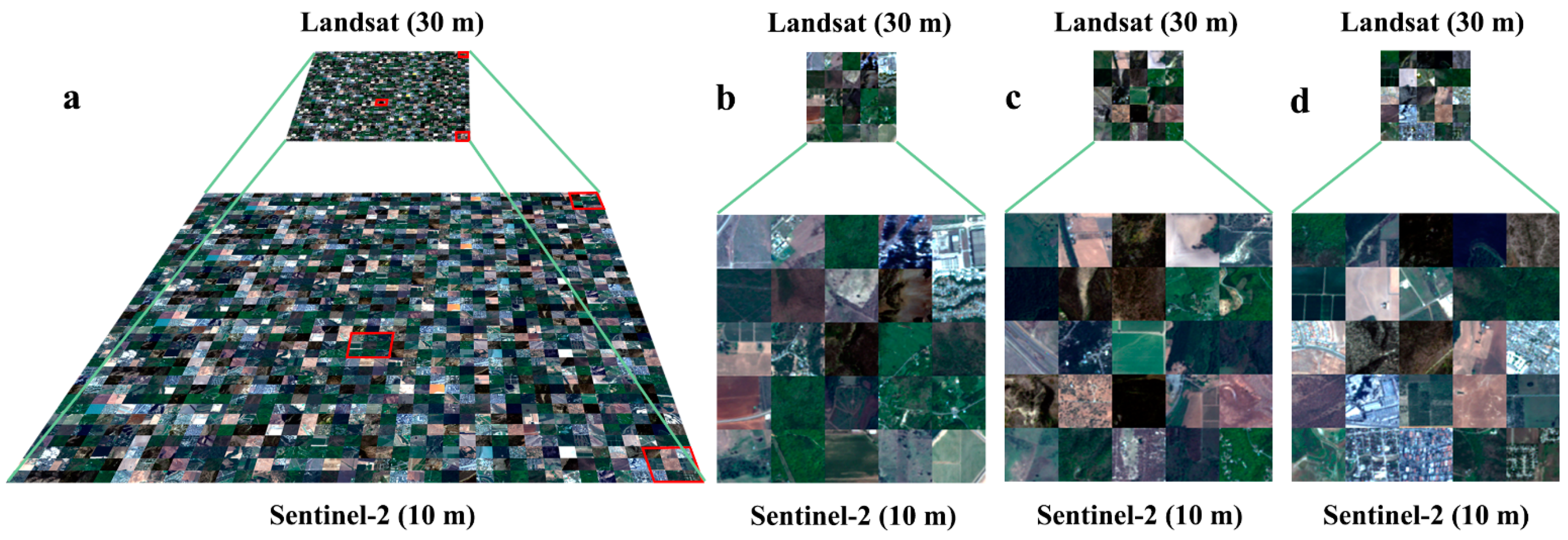
We extracted the overlapping areas for each pair of Landsat and Sentinel-2 imagery, and further cropped them into patch-based Landsat and Sentinel-2 imagery pairs with a unified patch size (160 × 160 for Landsat and 480 × 480 for Sentinel-2 in this study). These cropped subsets of Landsat and Sentinel-2 imagery pairs (Figure 4) were then used as input of the CNN models.
We collected three additional groups of datasets for time-series super-resolution experiments in capturing intra-annual land cover dynamics with fine spatial resolutions (Table 2). We acquired a series of Landsat-8 imagery in the states of Massachusetts and California to enhance their spatial resolutions to better capture phenology changes over vegetated area, cropping rotations over agricultural areas, and water dynamics over reservoirs.
To test the ultimate goal of transforming 30 m historical Landsat to 10 m Sentinel-like archive, we selected Schonefeld, Dubai, and Las Vegas as worldwide experimental sites (Figure 3b) to super-resolve annual Landsat imagery from 1985 to 2018.

3. Experimental Tests and Results

3.1. Tests with Simulated Data

In this experiment, cropped Sentinel-2 images with the size of 480 × 480 × 3 were used as IHR images. The corresponding ILR images (160 × 160 × 3) were obtained by upscaling Sentinel-2 images by a factor of three with the bicubic interpolation. A total of 1220 ILRIHR image pairs were randomly split, with 90% of them used for training and 10% for validation. It should be noted that the validation dataset was used to provide an unbiased evaluation while tuning model hyperparameters. A selection of an additional 57 testing images were used to evaluate the final model performance.
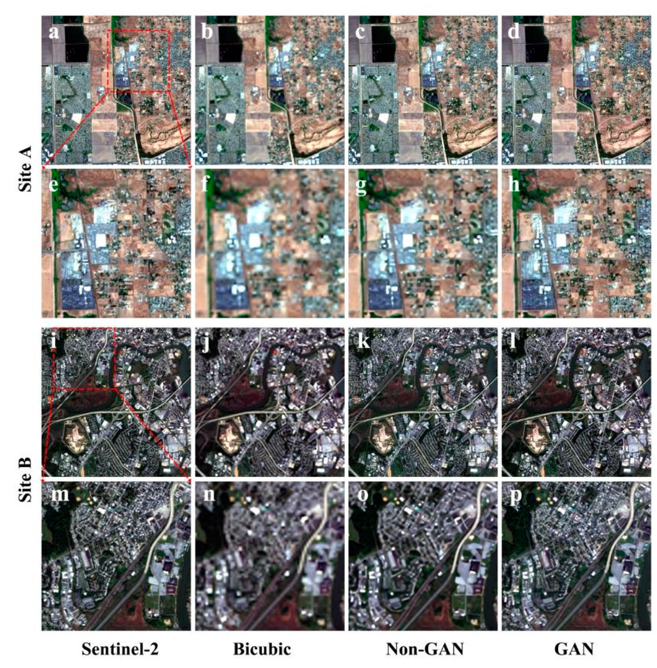
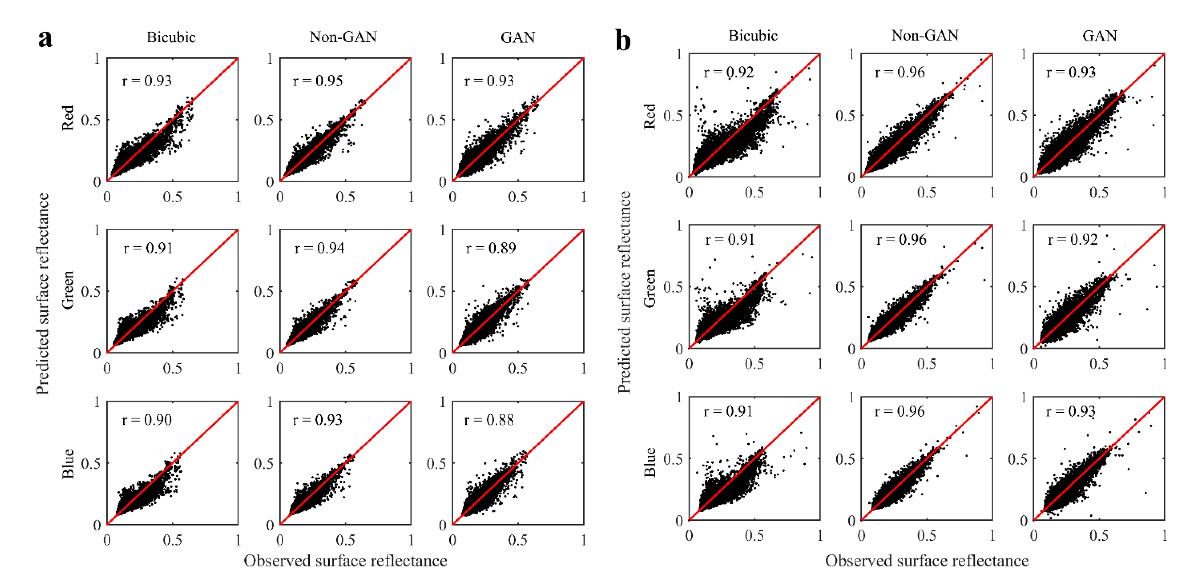
We selected two sites out of the 57 testing images to visually compare the spatial details and spectral fidelity between the original Sentinel-2 image and reconstructed 10 m Sentinel-2-like images (Figure 5). Compared with the reference images (Figure 5a,i), the interpolation from the upscaling Sentinel-2 image (Figure 5b,j), non-GAN-based method (Figure 5c,k) and GAN-based method (Figure 5d,l) had very similar spectral characteristics. The scatterplots of the red–green–blue bands between the reference and reconstructed images at site A (Figure 6a) and site B (Figure 6b) quantitatively verified their high correlation in spectral signatures. Non-GAN derived images (r = 0.94 for site A and r = 0.96 for site B) achieved comparably higher correlation than both the interpolated (r = 0.91 for site A and r = 0.91 for site B) images and the GAN derived images (r = 0.90 for site A and r = 0.93 for site B). In contrast to the similar spectral characteristics, the reconstructed spatial details were considerably different among these methods. Compared with the true reference (Figure 5e,m), the interpolated images (Figure 5f,n) were very blurred, and it was very difficult to identify the exact road network and infrastructure edges. As shown in the zoomed-in subsets for both sites (Figure 5e–h,m–p). In contrast, the non-GAN derived images (Figure 5g,o) improved the spatial details to a certain degree, but blurring effects still existed. The GAN derived images (Figure 5h,p), on the other hand, retained the fine-resolution spatial details that were nearly identical to the original Sentinel-2 images. For example, the road network, building edges, and land parcel blocks identified from the original and reconstructed ones were quite similar through visual inspections.
We used a group of full-reference indices including quality index (QI) [44], PSNR, root-mean-square-error (RMSE), and ERGAS [45], and non-reference indices including NIQE [46], PIQE [47], and BRISQUE [46] to assess the model performance of the 57 testing images. Based on the quantitative measures (Table 3), non-GAN approach achieved a slightly better performance in retaining spectral fidelity than the traditional interpolation and GAN approach. In contrast, the non-reference indices revealed that the GAN derived results had much better spatial details than the interpolated and non-GAN derived results. For example, the score of the indicators such as NIQE, PIQE, and BRISQUE from GAN derived results were much lower than those from the interpolated and non-GAN derived results.

3.2. Tests with Real Data

Different from the simulated data experiment in Section 3.1, Landsat images were directly used as ILR and Sentinel-2 images were used as IHR in this experiment. Similarly, we used 90% out of 1220 Landsat and Sentinel-2 ILRIHR image pairs for training, 10% for validation, and an additional 57 image pairs for testing the final model performance. In addition to the interpolated and non-GAN derived methods, we included another five methods as baselines to compare against, including the smoothing filter based intensity modulation (SFIM) [48], high pass filtering (HPF) [49], band-dependent spatial-detail (BDSD) [50], area-to-point regression kriging (ATPRK) [31,51], and target-adaptive CNN-based (TCNN) algorithms [52,53]. The selected five methods all required the guidance of 10 m Sentinel-2 imagery to downscale the corresponding 30 m Landsat imagery.
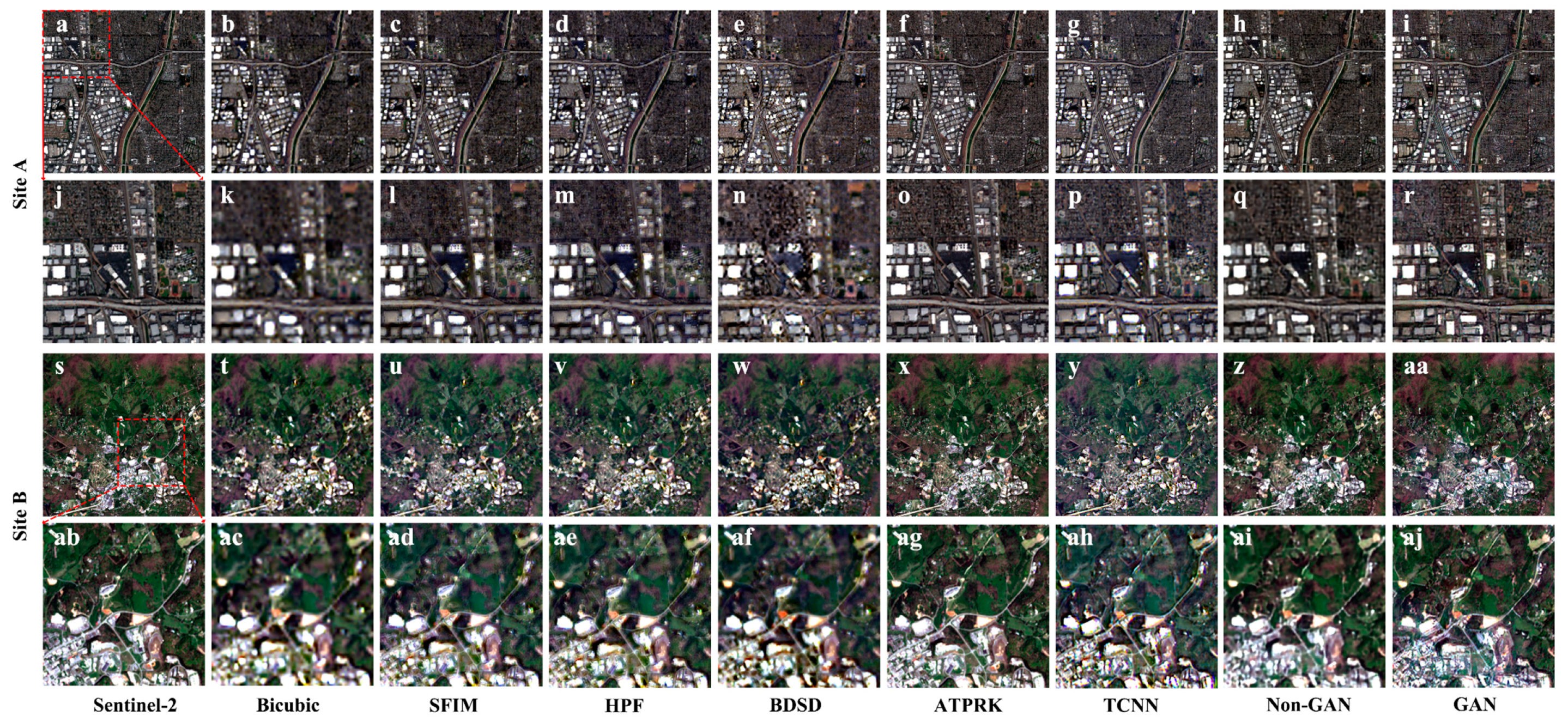
We again selected two sites out of the 57 testing images to visually compare the original Sentinel-2 image and reconstructed 10 m Sentinel-2-like images (Figure 7). The spectral signatures of the reference images, the interpolated Landsat, SFIM derived, HPF derived, BDSD derived, ATPRK derived, TCNN derived, non-GAN derived, and GAN derived 10-m Sentinel-2 images were similar in general (Figure 7). However, we could still identify the obvious spectral distortions from the SFIM, HPF, and BSSD derived results (Figure 7c–e,u–w). In contrast, the reconstructed images showed considerable differences in spatial details, which was reflected from the zoomed-in subsets in Figure 7j–r for site A and Figure 7ab–aj for site B. The derived images from the ATPRK, TCNN, and GAN methods retained the fine spatial details relatively well. The reconstructed images were almost identical to the original Sentinel-2 images; we could clearly identify the building blocks and roads.
We used the same set of quantitative measures to assess the model performance of the 57 testing images in a real-data experiment. The quantitative results (Table 4) revealed that the non-GAN-based model was better at retaining spectral fidelity, while the GAN-based model could construct more detailed spatial high frequency patterns. Noticeably, the ATPRK based model also achieved a comparable performance in persevering spatial and spectral information. However, it should be noted that the implementation of SFIM, HPF, BDSD and ATPRK models requires the input of corresponding Sentinel-2 images as the downscaling guidance, whereas the input of non-GAN and GAN-based models is only the 30 m Landsat imagery. On this basis, results shown in Figure 7 and Table 4 further reinforce the potential value of our proposed methods.

3.3. Tests with Time-Series Data

We further applied the GAN-based model trained from the real data in Section 3.2 to the time series of Landsat imagery across different landscapes, in order to test its performance of capturing inter-annual land cover dynamics, including phenology changes over vegetated area, cropping rotations over agricultural area, and water dynamics.
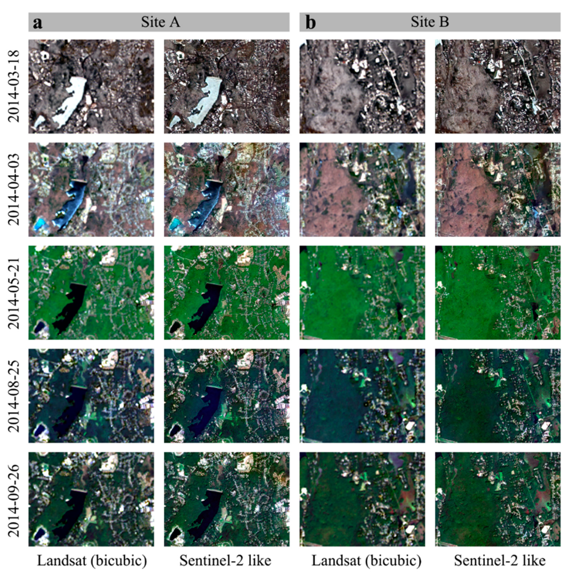
A selection of cloud-free Landsat-8 imagery was acquired in Massachusetts, where seasonal phenology changes are significant (Figure 8). The major land-cover types were forest, grass, water, bare land, and buildings for both sites A and B. Compared with the interpolated Landsat images (left panels of Figure 8a,b), the reconstructed Sentinel-2 like images (right panels of Figure 8a,b) greatly improved the spatial details while preserving spectral consistency.
A selection of monthly Landsat-8 imagery from January to October was acquired in California, where agricultural activities were dominant and cropping rotation was frequent (Figure 9). By applying the GAN-based model, we derived the corresponding 10 m Sentinel-2-like images (right panels of Figure 9. Results showed that the reconstructed images accurately captured crop phenology changes and depicted double cropping rotations (i.e., the first was from January to April, and second was from May to October). Given the relative homogeneity of land cover types in this region, the enhanced spatial details of reconstructed Sentinel-2-like images did not show considerable differences from those of the interpolated Landsat images through visual inspections. However, the intra-class difference in growing status and phenology changes could be easily identified from the reconstructed Senitnel-2-like images, whereas this was very difficult from the interpolated Landsat images.
An additional selection of monthly Landsat-8 imagery from January to October was acquired in California, where water bodies were dominant, with certain changes in spatial coverage and water colors (Figure 10). Compared with the interpolated Landsat images (left panels of Figure 10), the reconstructed Sentinel-2-like images (right panels of Figure 10) captured spatial details much more accurately without any blurring effects. For example, the inundation areas on August 18 and September 3 were depicted with fine spatial details in both intra-class variation and adjacent boundaries for Sentinel-2-like images, while the corresponding Landsat images only captured the general distribution of inundations with obvious blurs.

3.4. Reconstruction of 10 m Historical Landsat Archive

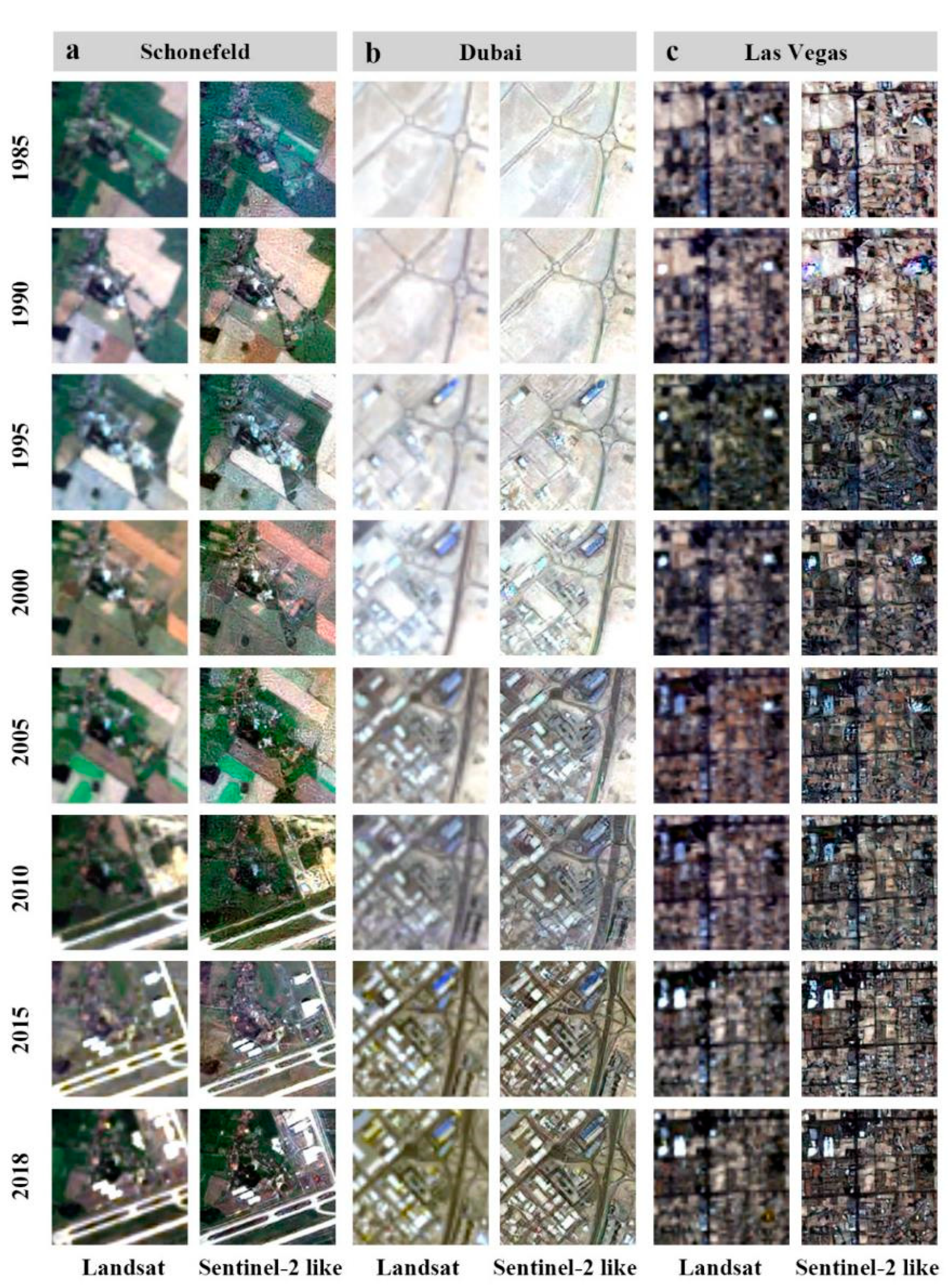
To address our ultimate goal of transforming 30 m historical Landsat images to a 10 m Sentinel-2-like archive, we acquired annual Landsat imagery from 1985 to 2018 in Schonefeld, Dubai, and Las Vegas (Figure 3b), where land cover changes were extreme (Figure 11). In Schonefeld, Germany, cropland was converted into artificial impervious areas for airport construction. In Dubai, United Arab Emirates, coastal expansion was tremendous, with the creation of Palm Islands and extreme urbanization. In Las Vegas, U.S.A., bare lands were rapidly converted to urbanized areas over the past decades. We applied the GAN-based models to generate the time-series 10 m Sentinel-2-like images over the selected three regions. Given the fact that there were no real 10 m Sentinel-2 images available before 2015, we visually compared the image quality in terms of spectral fidelity and spatial details between the interpolated Landsat and the reconstructed Sentinel-2-like images. As shown by the derived results with five-year intervals from 1985 to 2018 in Figure 11, the reconstructed images preserved consistent spectral fidelity and achieved plausible spatial details. We could also identify the very close spatial details between the predicted Sentinel-2-like imagery and the observed Sentinel-2 imagery in 2018. The zoomed-in comparison (Figure 12) further demonstrated that the improvement of spatial details using the GAN-based model was very obvious and robust over the long-term temporal period. For example, the road networks, building infrastructures, and street blocks were quite blurred in original Landsat images (left panels of Figure 12a–c), whereas they turned out to be quite clear in the reconstructed Sentinel-2-like images (right panels of Figure 12a–c).

4. Discussion

4.1. Training and Tuning of Deep Learning Models

Deep learning approaches are always complex in terms of neural network structures. They may be sensitive to the training and tuning process and the performance may vary on landscapes with varying spatial heterogeneity and temporal dynamics. These pose challenges for fusing remote sensing imagery with multispectral and multiscale observations. Here, we briefly discuss four important aspects of applying non-GAN and GAN-based deep learning SR models, including the training dataset, model generalization ability, potential benefit from transfer learning, and the impact of the number of iterations.
Firstly, training data are a key component to the machine learning algorithms that depend on the input reference and memorize the statistical and structured information for future predictions. Models usually perform better on the test set that have similar distribution as the training set. Therefore, the increase in the number and variability of training samples typically leads to better performance of the deep learning models. This calls for future efforts to expand and consolidate the regional to global training library that covers more comprehensive land use/cover type and changes.
Secondly, the model generalization ability describes a model’s ability to make accurate predictions on the new dataset that it has never encountered during the training. It is a key element of a successful and robust model. In this study, a number of Landsat and Sentinel-2 imagery pairs were collected across different landscapes in the United States. In Section 3.1 and Section 3.2, although training and testing datasets were randomly split without any overlapped information, they shared similar land cover types between adjacent locations. Therefore, similar patterns from training could be well transferred to the test dataset, making predictions over the testing data less challenging. However, the test dataset collected in the experiments using seasonal and long-term time-series imagery (Section 3.3 and Section 3.4) was totally independent from the training dataset; our model performed similarly and was able to accurately predict and capture the land-cover dynamics with high spectral fidelities and spatial details, demonstrating that our model generalizes very well. It further verified the possibility of leveraging limited samples of Landsat and Sentinel-2 observations during their overlapping period from 2016 to 2019 to transform 30 m historical Landsat images into a 10 m Sentinel-2-like archive.
Thirdly, transfer learning which makes use of all parameters of neural network pre-trained over large datasets has been proven to be quite helpful and efficient to solve a different but related problem [54]. It usually has the advantage of using fewer training samples and time while obtaining better results. To test whether remote sensing super-resolution could benefit from initial weights based on a model pre-trained from a natural image dataset, we conducted a group of experimental tests. In this experiment, the GAN-based network were first trained on DIV2K dataset [55], and then fine-tuned using remote sensing images at a smaller learning rate of 10−5, because the setting of a smaller learning rate performs better in fine-tuning. Comparative results revealed that the integration of natural images did not improve model performance (Figure S1, Table S2). This can be attributed to the difference in spectral wavelength and spatial details between remote sensing imagery and natural images.
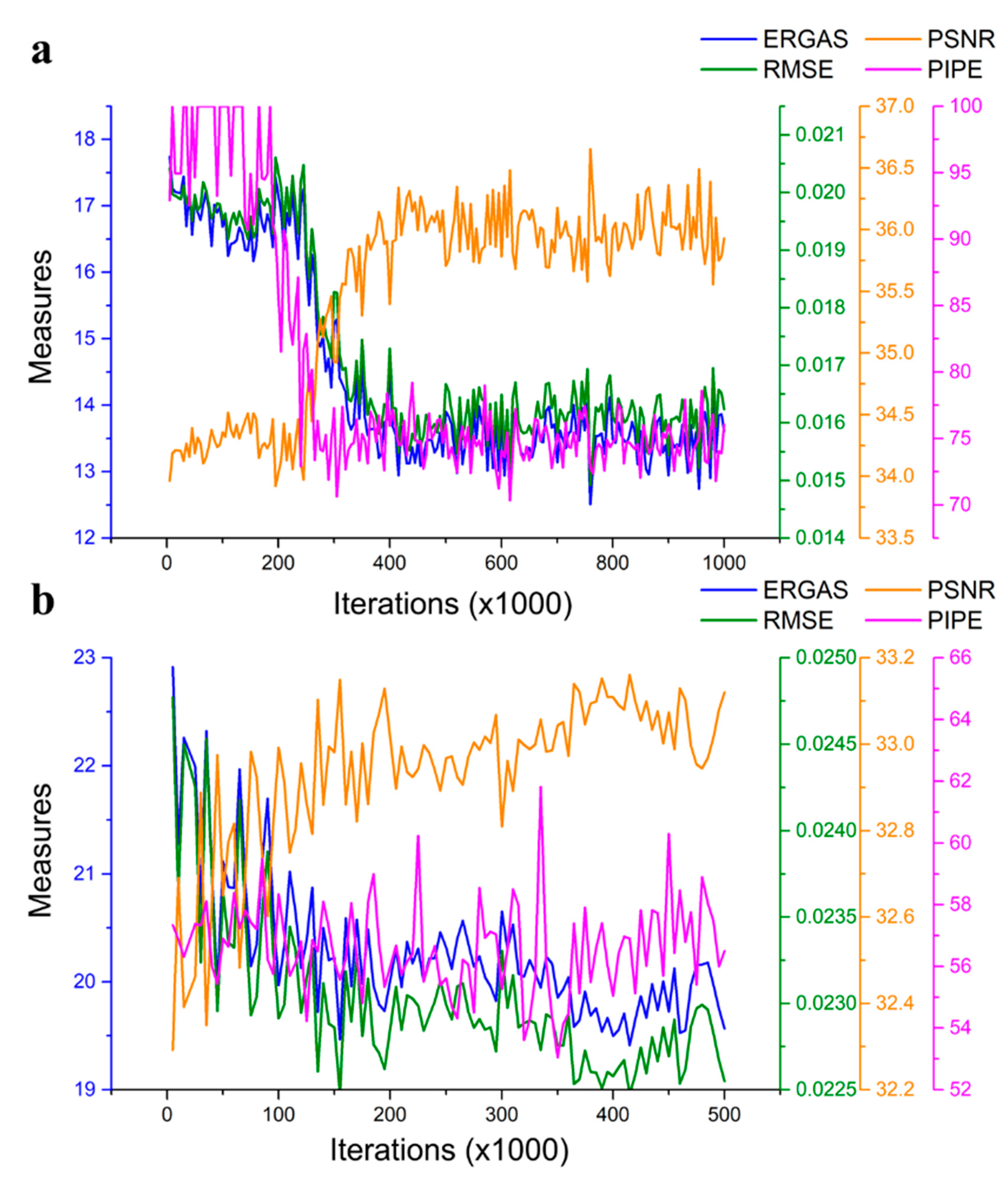
Finally, the number of iterations is another critical issue that influences deep learning-based model accuracy. As shown in Figure 13a, the accuracy of the non-GAN based model was relatively much lower with 5000 to 200,000 iterations, increased rapidly with the increasing number of iterations, and then became stable with more than 400,000 iterations. Similar patterns were found for GAN-based models (Figure 13b). We noticed that the GAN-based model was less stable when compared to the non-GAN-based model, which reflects the fact that GAN is more sensitive to training than a normal deep CNN [32]. The sensitivity analysis provided some semi-empirical knowledge that could be very helpful in training and tuning the optimal deep learning models.

4.2. Future Prospect

There are so far no existing algorithms that can produce super-resolution images with both high quantitative accuracy and high perceptual quality at the same time. Non-GAN based methods, optimizing the pixel-wise reconstruction measure, tend to produce over-smoothed images that lack high-frequency textures, and have also been shown to correlate poorly with human perception [34,56]. In contrast, GAN-based methods achieve very good performance in reconstructing high-frequency spatial details but are often inferior in terms of distortion measure [34,39,56,57]. This leads to a common perception–distortion trade-off phenomenon. On one hand, the balance of quantitative accuracy and spatial details can be application-oriented depending on the specific purpose. On the other hand, although this trade-off cannot be addressed thoroughly [58], future work can be conducted to alleviate this dilemma. For example, in our model generator design, adding an L1 regularization term to take the pixel level differences between the true and generated images into account forced the generated super-resolved images close to its corresponding I H R . Therefore, the accuracy increased, while the perceptual quality was preserved. Designing more advanced loss functions is also another promising direction.
We applied the GAN-based super-resolution algorithm to leverage Landsat and Sentinel-2 observations during their overlapping period from 2016 to 2019 for transforming 30 m historical Landsat images into a 10 m Sentinel-2-like archive. Although the experimental results in both intra- and inter-annual scales showed robust performance of our proposed method (Figure 8, Figure 9, Figure 10, Figure 11 and Figure 12), our methods and results should be interpreted in light of certain uncertainties. Firstly, the difference in sensors, observation geometries, and image quality may lead to potential biases in spatial details and spectral fidelity of the time-series reconstructed Landsat imagery. For example, the possible lower image quality of the input data, e.g., due to cloud/shadow contaminations and geometry distortions, may cause errors especially for long-term temporal reconstruction applications. In addition, although our proposed methods can be easily extended to other sensors such as National Agriculture Imagery Program (NAIP) imagery (Figure S2), RapidEye, and PlanetScope datasets, careful consideration should be made with regard to the scale discrepancy between two paired images. In this study, with a factor of three between the Landsat and Sentinel-2 pixel sizes, the reconstruction of super-resolution worked very well. However, if the scale difference is larger than eight, the single-image super-resolution may yield unrealistic and blurred results [59]. In this situation, we may use medium-resolution images between the coarse- and high-resolution images as the bridge to close the scale gap.
Despite these uncertainties, our study demonstrated that the fusion methods developed here and corresponding reconstructed Sentinel-2-like archive are very promising, and can be applied to a variety of other applications, such as urban, forest, wetland, wildfires, land cover classification and change detection. Potentially, all research and applications that traditionally rely on Landsat but require higher spatial details can be enhanced with the support of our feature-level fusion methods and resulting reconstructed Sentinel-2-like data archive.

5. Conclusions

Fine spatial resolution Earth observation images are desirable for much environmental change and land management research. However, the investigation of long-term terrestrial change has mostly relied on 30 m moderate-resolution Landsat imagery. This study sought to leverage Landsat and Sentinel-2 observations during their overlapping period from 2016 to more up-to-date images, to reconstruct 10 m Sentinel-2-like imagery from 30 m historical Landsat data since the Sentinel-2 era, and potentially over the past four decades. To achieve this goal, we presented a generative adversarial network (GAN) based data fusion framework that blended fine-resolution feature-level spatial information from Sentinel-2, to enhance the spatial resolution of the historical Landsat archive. We conducted a set of experimental tests using simulated data, actual Landsat/Sentinel-2 acquisitions, and time-series Landsat imagery. Our results showed Landsat data which were reconstructed to 10 m using a GAN-based super-resolution method, accurately captured the spatial features at an effective resolution close to Sentinel-2 observations. Historical reconstruction of 10 m Landsat observations from 1985 to 2018 in three different types of landscape changes further verified the robustness and efficiency of our proposed method for monitoring land changes. The promising results from our deep learning-based feature-level fusion method highlight the potential for reconstructing a 10 m Landsat series archive since 1984. The enhanced Landsat and Sentinel-2 data is expected to improve our capability of detecting and tracking finer scale land changes, identifying the drivers for and responses to global environmental changes, and designing better land management policies and strategies.

Supplementary Materials

The following are available online at https://www.mdpi.com/2072-4292/13/2/167/s1, Figure S1 Super-resolution results in the real data experiment. From left to right: original Sentinel-2, interpolated, Non-GAN derived (RS only), GAN derived (RS only), Non-GAN derived (RS & natural images), and GAN derived (RS & natural images) images at the site A (a-l) and site B (m-x). For site A, (g-l) are shown as the zoomed-in comparison of (a-f); for site B, (s-x) are shown as the zoomed-in comparison of (m-r). Figure S2. Super-resolution results using NAIP imagery. The reference high-resolution images from NAIP-0.6m are shown on the left. On the right are zoomed-in subsets of the yellow box from original reference, bicubic interpolation, Non-GAN derived, and GAN-derived results. Table S1. Comparison of Landsat and Sentinel-2 bandwidth. Table S2. Accuracy assessment of two training scenarios in actual experiment.

Author Contributions

Conceptualization, B.C. and Y.J.; methodology, B.C. and J.L.; software, B.C. and J.L.; validation, B.C. and J.L.; formal analysis, B.C. and J.L.; investigation, B.C. and J.L.; resources, B.C. and J.L.; data curation, B.C.; writing—original draft preparation, B.C. and J.L.; writing—review and editing, B.C. and Y.J.; visualization, B.C.; supervision, Y.J.; project administration, Y.J.; funding acquisition, Y.J. All authors have read and agreed to the published version of the manuscript.

Funding

This research was supported by CaliforniaView under the USGS AmericaView grant and the Innovation Center for Advancing Ecosystem Climate Solutions funded by California Strategic Growth Council.

Institutional Review Board Statement

Not Applicable.

Informed Consent Statement

Not applicable.

Data Availability Statement

Not applicable.

Conflicts of Interest

The authors declare no conflict of interest.

References

  1. Allen, C.D. Interactions across spatial scales among forest dieback, fire, and erosion in northern New Mexico landscapes. Ecosystems 2007, 10, 797–808. [Google Scholar] [CrossRef] [Green Version]
  2. Lepers, E.; Lambin, E.F.; Janetos, A.C.; DeFries, R.; Achard, F.; Ramankutty, N.; Scholes, R.J. A synthesis of information on rapid land-cover change for the period 1981–2000. BioScience 2005, 55, 115–124. [Google Scholar] [CrossRef]
  3. Roy, D.P.; Wulder, M.A.; Loveland, T.R.; Woodcock, C.E.; Allen, R.G.; Anderson, M.C.; Helder, D.; Irons, J.R.; Johnson, D.M.; Kennedy, R. Landsat-8: Science and product vision for terrestrial global change research. Remote Sens. Environ. 2014, 145, 154–172. [Google Scholar] [CrossRef] [Green Version]
  4. Wulder, M.A.; Loveland, T.R.; Roy, D.P.; Crawford, C.J.; Masek, J.G.; Woodcock, C.E.; Allen, R.G.; Anderson, M.C.; Belward, A.S.; Cohen, W.B. Current status of Landsat program, science, and applications. Remote Sens. Environ. 2019, 225, 127–147. [Google Scholar] [CrossRef]
  5. Wulder, M.A.; White, J.C.; Goward, S.N.; Masek, J.G.; Irons, J.R.; Herold, M.; Cohen, W.B.; Loveland, T.R.; Woodcock, C.E. Landsat continuity: Issues and opportunities for land cover monitoring. Remote Sens. Environ. 2008, 112, 955–969. [Google Scholar] [CrossRef]
  6. Chen, B.; Huang, B.; Chen, L.; Xu, B. Spatially and temporally weighted regression: A novel method to produce continuous cloud-free Landsat imagery. IEEE Trans. Geosci. Remote Sens. 2016, 55, 27–37. [Google Scholar] [CrossRef]
  7. Grimmond, S.U. Urbanization and global environmental change: Local effects of urban warming. Geogr. J. 2007, 173, 83–88. [Google Scholar] [CrossRef]
  8. Theobald, D.M.; Kennedy, C.; Chen, B.; Oakleaf, J.; Baruch-Mordo, S.; Kiesecker, J. Earth transformed: Detailed mapping of global human modification from 1990 to 2017. Earth Syst. Sci. Data 2020, 12, 1953–1972. [Google Scholar] [CrossRef]
  9. Michishita, R.; Jiang, Z.; Xu, B. Monitoring two decades of urbanization in the Poyang Lake area, China through spectral unmixing. Remote Sens. Environ. 2012, 117, 3–18. [Google Scholar] [CrossRef]
  10. Zhang, L.; Weng, Q. Annual dynamics of impervious surface in the Pearl River Delta, China, from 1988 to 2013, using time series Landsat imagery. ISPRS J. Photogramm. Remote Sens. 2016, 113, 86–96. [Google Scholar] [CrossRef]
  11. Chen, B.; Jin, Y.; Brown, P. An enhanced bloom index for quantifying floral phenology using multi-scale remote sensing observations. ISPRS J. Photogramm. Remote Sens. 2019, 156, 108–120. [Google Scholar] [CrossRef]
  12. Belgiu, M.; Csillik, O. Sentinel-2 cropland mapping using pixel-based and object-based time-weighted dynamic time warping analysis. Remote Sens. Environ. 2018, 204, 509–523. [Google Scholar] [CrossRef]
  13. Gilbertson, J.K.; Kemp, J.; Van Niekerk, A. Effect of pan-sharpening multi-temporal Landsat 8 imagery for crop type differentiation using different classification techniques. Comput. Electr. Agric. 2017, 134, 151–159. [Google Scholar] [CrossRef] [Green Version]
  14. Gong, P.; Chen, B.; Li, X.; Liu, H.; Wang, J.; Bai, Y.; Chen, J.; Chen, X.; Fang, L.; Feng, S. Mapping essential urban land use categories in China (EULUC-China): Preliminary results for 2018. Sci. Bull. 2020, 65, 182–187. [Google Scholar] [CrossRef] [Green Version]
  15. Mahdianpari, M.; Salehi, B.; Mohammadimanesh, F.; Homayouni, S.; Gill, E. The first wetland inventory map of newfoundland at a spatial resolution of 10 m using Sentinel-1 and Sentinel-2 data on the Google Earth Engine cloud computing platform. Remote Sens. 2019, 11, 43. [Google Scholar] [CrossRef] [Green Version]
  16. Drusch, M.; Del Bello, U.; Carlier, S.; Colin, O.; Fernandez, V.; Gascon, F.; Hoersch, B.; Isola, C.; Laberinti, P.; Martimort, P. Sentinel-2: ESA’s optical high-resolution mission for GMES operational services. Remote Sens. Environ. 2012, 120, 25–36. [Google Scholar] [CrossRef]
  17. Korhonen, L.; Packalen, P.; Rautiainen, M. Comparison of Sentinel-2 and Landsat 8 in the estimation of boreal forest canopy cover and leaf area index. Remote Sens. Environ. 2017, 195, 259–274. [Google Scholar] [CrossRef]
  18. Chen, B.; Huang, B.; Xu, B. Comparison of spatiotemporal fusion models: A review. Remote Sens. 2015, 7, 1798–1835. [Google Scholar] [CrossRef] [Green Version]
  19. Gao, F.; Masek, J.; Schwaller, M.; Hall, F. On the blending of the Landsat and MODIS surface reflectance: Predicting daily Landsat surface reflectance. IEEE Trans. Geosci. Remote Sens. 2006, 44, 2207–2218. [Google Scholar]
  20. Zhu, X.; Chen, J.; Gao, F.; Chen, X.; Masek, J.G. An enhanced spatial and temporal adaptive reflectance fusion model for complex heterogeneous regions. Remote Sens. Environ. 2010, 114, 2610–2623. [Google Scholar] [CrossRef]
  21. Li, S.; Kwok, J.T.; Wang, Y. Using the discrete wavelet frame transform to merge Landsat tm and spot panchromatic images. Inf. Fusion 2002, 3, 17–23. [Google Scholar] [CrossRef]
  22. Li, S.; Yang, B. A new pan-sharpening method using a compressed sensing technique. IEEE Trans. Geosci. Remote Sens. 2010, 49, 738–746. [Google Scholar] [CrossRef]
  23. Zhang, H.K.; Roy, D.P. Computationally inexpensive Landsat 8 operational land imager (OLI) pansharpening. Remote Sens. 2016, 8, 180. [Google Scholar] [CrossRef] [Green Version]
  24. Huang, B.; Song, H. Spatiotemporal reflectance fusion via sparse representation. IEEE Trans. Geosci. Remote Sens. 2012, 50, 3707–3716. [Google Scholar] [CrossRef]
  25. Luo, Y.; Guan, K.; Peng, J. Stair: A generic and fully-automated method to fuse multiple sources of optical satellite data to generate a high-resolution, daily and cloud-/gap-free surface reflectance product. Remote Sens. Environ. 2018, 214, 87–99. [Google Scholar] [CrossRef]
  26. Shen, H.; Huang, L.; Zhang, L.; Wu, P.; Zeng, C. Long-term and fine-scale satellite monitoring of the urban heat island effect by the fusion of multi-temporal and multi-sensor remote sensed data: A 26-year case study of the city of Wuhan in china. Remote Sens. Environ. 2016, 172, 109–125. [Google Scholar] [CrossRef]
  27. Weng, Q.; Fu, P.; Gao, F. Generating daily land surface temperature at Landsat resolution by fusing Landsat and MODIS data. Remote Sens. Environ. 2014, 145, 55–67. [Google Scholar] [CrossRef]
  28. Shao, Z.; Cai, J.; Fu, P.; Hu, L.; Liu, T. Deep learning-based fusion of Landsat-8 and Sentinel-2 images for a harmonized surface reflectance product. Remote Sens. Environ. 2019, 235, 111425. [Google Scholar] [CrossRef]
  29. Yan, L.; Roy, D.P. Spatially and temporally complete Landsat reflectance time series modelling: The fill-and-fit approach. Remote Sens. Environ. 2020, 241, 111718. [Google Scholar] [CrossRef]
  30. Claverie, M.; Ju, J.; Masek, J.G.; Dungan, J.L.; Vermote, E.F.; Roger, J.-C.; Skakun, S.V.; Justice, C. The harmonized Landsat and Sentinel-2 surface reflectance data set. Remote Sens. Environ. 2018, 219, 145–161. [Google Scholar] [CrossRef]
  31. Wang, Q.; Blackburn, G.A.; Onojeghuo, A.O.; Dash, J.; Zhou, L.; Zhang, Y.; Atkinson, P.M. Fusion of Landsat 8 OLI and Sentinel-2 MSI data. IEEE Trans. Geosci. Remote Sens. 2017, 55, 3885–3899. [Google Scholar] [CrossRef] [Green Version]
  32. Goodfellow, I.; Bengio, Y.; Courville, A.; Bengio, Y. Deep Learning; MIT Press: Cambridge, MA, USA, 2016; Volume 1. [Google Scholar]
  33. Kim, J.; Kwon Lee, J.; Mu Lee, K. Accurate Image Super-Resolution Using Very Deep Convolutional Networks. In Proceedings of the IEEE Conference on Computer Vision and Pattern Recognition, Las Vegas, NV, USA, 27–30 June 2016; pp. 1646–1654. [Google Scholar]
  34. Ledig, C.; Theis, L.; Huszár, F.; Caballero, J.; Cunningham, A.; Acosta, A.; Aitken, A.; Tejani, A.; Totz, J.; Wang, Z. Photo-realistic single image super-resolution using a generative adversarial network. In Proceedings of the IEEE Conference on Computer Vision and Pattern Recognition, Honolulu, HI, USA, 21–26 July 2017; pp. 4681–4690. [Google Scholar]
  35. Dong, C.; Loy, C.C.; He, K.; Tang, X. Image super-resolution using deep convolutional networks. IEEE Trans. Pattern Anal. Mach. Intell. 2015, 38, 295–307. [Google Scholar] [CrossRef] [Green Version]
  36. Pouliot, D.; Latifovic, R.; Pasher, J.; Duffe, J. Landsat super-resolution enhancement using convolution neural networks and sentinel-2 for training. Remote Sens. 2018, 10, 394. [Google Scholar] [CrossRef] [Green Version]
  37. Zhang, Y.; Tian, Y.; Kong, Y.; Zhong, B.; Fu, Y. Residual dense network for image super-resolution. In Proceedings of the IEEE Conference on Computer Vision and Pattern Recognition, Salt Lake City, UT, USA, 18–22 June 2018; pp. 2472–2481. [Google Scholar]
  38. Lim, B.; Son, S.; Kim, H.; Nah, S.; Mu Lee, K. Enhanced deep residual networks for single image super-resolution. In Proceedings of the IEEE Conference on Computer Vision and Pattern Recognition Workshops, Honolulu, HI, USA, 21–26 July 2017; pp. 136–144. [Google Scholar]
  39. Johnson, J.; Alahi, A.; Fei-Fei, L. Perceptual losses for real-time style transfer and super-resolution. In Proceedings of the European Conference on Computer Vision, Amsterdam, The Netherlands, 8–16 October 2016; Springer: Amsterdam, The Netherlands, 2016; pp. 694–711. [Google Scholar]
  40. Lanaras, C.; Bioucas-Dias, J.; Galliani, S.; Baltsavias, E.; Schindler, K. Super-resolution of sentinel-2 images: Learning a globally applicable deep neural network. ISPRS J. Photogramm. Remote Sens. 2018, 146, 305–319. [Google Scholar] [CrossRef] [Green Version]
  41. Goodfellow, I.; Pouget-Abadie, J.; Mirza, M.; Xu, B.; Warde-Farley, D.; Ozair, S.; Courville, A.; Bengio, Y. Generative adversarial nets. In Proceedings of the Advances in Neural Information Processing Systems, Montreal, QC, Canada, 8–13 December 2014; pp. 2672–2680. [Google Scholar]
  42. Wang, X.; Yu, K.; Wu, S.; Gu, J.; Liu, Y.; Dong, C.; Qiao, Y.; Change Loy, C. Esrgan: Enhanced super-resolution generative adversarial networks. In Proceedings of the European Conference on Computer Vision (ECCV), Munich, Germany, 8–14 September 2018. [Google Scholar]
  43. Kingma, D.P.; Ba, J. Adam: A method for stochastic optimization. arXiv 2014, arXiv:1412.6980. [Google Scholar]
  44. Wang, Z.; Bovik, A.C. A universal image quality index. IEEE Signal Process. Lett. 2002, 9, 81–84. [Google Scholar] [CrossRef]
  45. Ranchin, T.; Aiazzi, B.; Alparone, L.; Baronti, S.; Wald, L. Image fusion—the arsis concept and some successful implementation schemes. ISPRS J. Photogramm. Remote Sens. 2003, 58, 4–18. [Google Scholar] [CrossRef] [Green Version]
  46. Mittal, A.; Soundararajan, R.; Bovik, A.C. Making a “completely blind” image quality analyzer. IEEE Signal Process. Lett. 2012, 20, 209–212. [Google Scholar] [CrossRef]
  47. Chan, R.W.; Goldsmith, P.B. A psychovisually-based image quality evaluator for jpeg images. In Proceedings of the 2000 IEEE International Conference on Systems, Man and Cybernetics, Nashville, TN, USA, 8–11 October 2000; pp. 1541–1546. [Google Scholar]
  48. Liu, J. Smoothing filter-based intensity modulation: A spectral preserve image fusion technique for improving spatial details. Int. J. Remote Sens. 2000, 21, 3461–3472. [Google Scholar] [CrossRef]
  49. Vivone, G.; Alparone, L.; Chanussot, J.; Dalla Mura, M.; Garzelli, A.; Licciardi, G.A.; Restaino, R.; Wald, L. A critical comparison among pansharpening algorithms. IEEE Trans. Geosci. Remote Sens. 2014, 53, 2565–2586. [Google Scholar] [CrossRef]
  50. Garzelli, A.; Nencini, F.; Capobianco, L. Optimal mmse pan sharpening of very high resolution multispectral images. IEEE Trans. Geosci. Remote Sens. 2007, 46, 228–236. [Google Scholar] [CrossRef]
  51. Wang, Q.; Shi, W.; Atkinson, P.M.; Zhao, Y. Downscaling MODIS images with area-to-point regression kriging. Remote Sens. Environ. 2015, 166, 191–204. [Google Scholar] [CrossRef]
  52. Masi, G.; Cozzolino, D.; Verdoliva, L.; Scarpa, G. Pansharpening by convolutional neural networks. Remote Sens. 2016, 8, 594. [Google Scholar] [CrossRef] [Green Version]
  53. Scarpa, G.; Vitale, S.; Cozzolino, D. Target-adaptive CNN-based pansharpening. IEEE Trans. Geosci. Remote Sens. 2018, 56, 5443–5457. [Google Scholar] [CrossRef] [Green Version]
  54. Weiss, K.; Khoshgoftaar, T.M.; Wang, D. A survey of transfer learning. J. Big Data 2016, 3, 9. [Google Scholar] [CrossRef] [Green Version]
  55. Agustsson, E.; Timofte, R. Ntire 2017 challenge on single image super-resolution: Dataset and study. In Proceedings of the IEEE Conference on Computer Vision and Pattern Recognition Workshops, Honolulu, HI, USA, 21–26 July 2017; pp. 126–135. [Google Scholar]
  56. Sajjadi, M.S.; Scholkopf, B.; Hirsch, M. Enhancenet: Single image super-resolution through automated texture synthesis. In Proceedings of the IEEE International Conference on Computer Vision, Venice, Italy, 22–29 October 2017; pp. 4491–4500. [Google Scholar]
  57. Dahl, R.; Norouzi, M.; Shlens, J. Pixel recursive super resolution. In Proceedings of the IEEE International Conference on Computer Vision, Venice, Italy, 22–29 October 2017; pp. 5439–5448. [Google Scholar]
  58. Blau, Y.; Michaeli, T. The perception-distortion tradeoff. In Proceedings of the IEEE Conference on Computer Vision and Pattern Recognition, Salt Lake City, UT, USA, 18–22 June 2018; pp. 6228–6237. [Google Scholar]
  59. Chen, B.; Huang, B.; Xu, B. A hierarchical spatiotemporal adaptive fusion model using one image pair. Int. J. Digit. Earth 2017, 10, 639–655. [Google Scholar] [CrossRef]
Figure 1. The architecture of the non-generative adversarial network (GAN)-based models. Note that the stride of 1 is applied to all convolutional layers.
Remotesensing 13 00167 g001
Figure 2. The architecture of GAN-based models.
Remotesensing 13 00167 g002
Figure 3. Sampled Landsat and Sentinel-2 scenes. (a) Paired Landsat-8 and Sentinel-2 imagery in the United States, and (b) worldwide experimental sites in Schonefeld, Dubai, and Las Vegas.
Remotesensing 13 00167 g003
Figure 4. The example mosaics of paired Landsat and Sentinel-2 imagery used for the training and validation process, in which area? (a). Details are also shown in (bd) for three example subsets highlighted in red squares in (a).
Remotesensing 13 00167 g004
Figure 5. Super-resolution results in the simulated data experiment. From left to right: original Sentinel-2, interpolated, non-GAN derived, and GAN derived images at site A (ah) and site B (ip). For site A, (eh) are shown as the zoomed-in comparison of (ad); for site B, (mp) are shown as the zoomed-in comparison of (il).
Remotesensing 13 00167 g005
Figure 6. Scatterplots of the predicted vs. observed surface reflectance (Sentinel-2) from the bicubic interpolation, non-GAN-based super-resolution, and GAN-based super-resolution, in terms of red, green, and blue bands at site A (a) and site B (b), as shown in Figure 5.
Remotesensing 13 00167 g006
Figure 7. Super-resolution results in the real data experiment. From left to right: original Sentinel-2, interpolated, smoothing filter based intensity modulation (SFIM) derived, high pass filtering (HPF) derived, band-dependent spatial-detail (BDSD) derived, area-to-point regression kriging (ATPRK) derived, target-adaptive CNN-based (TCNN) derived, non-GAN derived, and GAN derived images at the site A (ar) and site B (saj). For site A, (jr) are shown as the zoomed-in comparison of (ai); for site B, (abaj) are shown as the zoomed-in comparison of (saa).
Remotesensing 13 00167 g007
Figure 8. Super-resolution results of time-series Landsat images for capturing vegetation phenology over vegetated areas at site A (a) and site (b). From left to right: 10 m interpolation derived from Landsat using the bicubic method, and Sentinel-2-like reconstructed image derived from the GAN-based model.
Remotesensing 13 00167 g008
Figure 9. Super-resolution results of time-series Landsat images for capturing cropping rotations over agricultural land in California. From left to right: 10 m interpolation derived from Landsat using the bicubic method, Sentinel-2-like reconstructed image derived from the GAN-based super-resolution.
Remotesensing 13 00167 g009
Figure 10. Super-resolution results of time-series Landsat images for capturing water dynamics in California. From left to right: 10 m interpolation derived from Landsat using the bicubic method, and Sentinel-2-like reconstructed image derived from the GAN-based super-resolution.
Remotesensing 13 00167 g010
Figure 11. Historical reconstruction of 10 m Sentinel-2-like images in Schonefeld, Dubai, and Las Vegas from 1985 to 2018, and the corresponding Sentinel-2 observations in 2018.
Remotesensing 13 00167 g011
Figure 12. Zoomed-in comparison between Landsat and reconstructed 10 m Sentinel-2-like images in (a) Schonefeld, (b) Dubai, and (c) Las Vegas from 1985 to 2018.
Remotesensing 13 00167 g012
Figure 13. Sensitivity of training iterations to the model performance of (a) non-GAN and (b) GAN.
Remotesensing 13 00167 g013
Table 1. Acquisition tiles and dates of paired Landsat and Sentinel-2 imagery for experimental tests.
Landsat-8Sentinel-2 Landsat-8Sentinel-2
SceneDateSceneDateSceneDateSceneDate
#10440332016-07-1310SFH2016-07-14#70460292018-08-1810TDQ2018-08-19
#20440342016-07-1310SEG2016-07-14#80340322018-09-1513TDE2018-09-14
#30410362017-12-1811SLT2017-12-15#90380322018-11-1412TVL2018-11-14
#40210352018-04-2916SEF2018-04-28#100160412018-12-0617RML2018-12-05
#50190362018-05-0116SGD2018-04-30#110270402019-01-0114RNT2019-01-05
#60240302018-07-0715TYH2018-07-08
Table 2. Acquisition of Landsat-8 imagery for time-series super-resolution experiments.
Massachusetts (Scene: 012031)California (Scene: 043034)
#12014-03-18#12014-01-22#62014-06-15
#22014-04-03#22014-02-23#72014-07-01
#32014-05-21#32014-03-11#82014-08-18
#42014-08-25#42014-04-28#92014-09-03
#52014-09-26#52014-05-14#102014-10-05
Table 3. Model performance in the simulated data experiment assessed by full-reference and non-reference measures.
MeasuresBicubicNon-GANGAN
QI0.647 ± 0.0600.775 ± 0.0510.669 ± 0.066
PSNR39.197 ± 3.60041.977 ± 3.98739.391 ± 3.856
RMSE0.012 ± 0.0050.009 ± 0.0040.012 ± 0.005
ERGAS12.212 ± 3.9739.027 ± 3.29411.903 ± 4.266
NIQE5.995 ± 0.5074.839 ± 0.7762.911 ± 0.497
PIQE78.008 ± 8.49861.687 ± 9.04824.509 ± 14.898
BRISQUE52.079 ± 3.41340.553 ± 5.19425.257 ± 7.568
Table 4. Model performance in the real data experiment assessed by full-reference and non-reference measures.
MeasuresBicubicSFIMHPFBDSDATPRKTCNNNon-GANGAN
QI0.34 ± 0.100.65 ± 0.190.63 ± 0.100.57 ± 0.150.85 ± 0.070.54 ± 0.100.65 ± 0.140.37 ± 0.15
PSNR29.71 ± 1.7230.23 ± 1.5430.26 ± 1.5330.43 ± 1.3731.43 ± 1.3829.80 ± 1.8341.50 ± 6.0337.14 ± 5.75
RMSE0.04 ± 0.010.04 ± 0.010.03 ± 0.010.03 ± 0.010.03 ± 0.010.04 ± 0.010.01 ± 0.010.02 ± 0.02
ERGAS76.97 ± 30.1975.30 ± 30.9074.83 ± 30.8073.63 ± 31.3371.06 ± 31.7374.00 ± 27.2412.03 ± 15.0918.66 ± 14.99
NIQE6.43 ± 0.814.45 ± 0.714.44 ± 0.664.50 ± 1.463.36 ± 0.753.79 ± 0.595.37 ± 0.863.40 ± 0.70
PIQE87.11 ± 11.8520.89 ± 11.0330.36 ± 11.5550.92 ± 24.6929.85 ± 11.7431.39 ± 11.8464.68 ± 12.4228.62 ± 11.37
BRISQUE52.63 ± 3.4630.45 ± 6.0435.09 ± 6.3242.71 ± 10.3531.28 ± 6.4331.70 ± 5.1144.25 ± 4.3730.27 ± 6.33
Publisher’s Note: MDPI stays neutral with regard to jurisdictional claims in published maps and institutional affiliations.