Abstract
Assessing crop production in the field often requires breeders to wait until the end of the season to collect yield-related measurements, limiting the pace of the breeding cycle. Early prediction of crop performance can reduce this constraint by allowing breeders more time to focus on the highest-performing varieties. Here, we present a multimodal deep learning model for predicting the performance of maize (Zea mays) at an early developmental stage, offering the potential to accelerate crop breeding. We employed multispectral images and eight vegetation indices, collected by an uncrewed aerial vehicle approximately 60 days after sowing, over three consecutive growing cycles (2017, 2018 and 2019). The multimodal deep learning approach was used to integrate field management and genotype information with the multispectral data, providing context to the conditions that the plants experienced during the trial. Model performance was assessed using holdout data, in which the model accurately predicted the yield (RMSE 1.07 t/ha, a relative RMSE of 7.60% of 16 t/ha, and R2 score 0.73) and identified the majority of high-yielding varieties, outperforming previously published models for early yield prediction. The inclusion of vegetation indices was important for model performance, with a normalized difference vegetation index and green with normalized difference vegetation index contributing the most to model performance. The model provides a decision support tool, identifying promising lines early in the field trial.
1. Introduction
Breeding crop varieties for improved performance in the field is costly and can encompass several years, as the individuals must be selected from large populations grown across multiple environments and years [1]. The prediction of end-of-season traits in the field can bypass the major time limitation imposed by the plant’s long life cycle, by allowing preliminary selection of the most promising individuals based on the plant phenotype at early developmental stages [2,3]. This would enable researchers to select a subset of the varieties to focus on, allowing the resources to be employed on collecting additional phenotyping measurements, sequencing the genome of selected individuals, or defining crossing plans for seed production [4]. High-throughput phenotyping (HTP) allows the monitoring of crop development and measuring plant traits under field or greenhouse conditions, using a wide range of sensors deployed on ground platforms, uncrewed aerial vehicles, or via satellite. The richness of HTP datasets enables breeders to explore features at a scale that was not previously feasible. For example, canopy temperature and a normalized difference vegetation index (NDVI) were shown to increase the accuracy of wheat (Triticum aestivum) genomic selection by 70%, using best linear unbiased prediction models (BLUP) [5]. In addition, plant spectral features collected using thermal, RGB, and multispectral sensors can be used to identify water-stressed individuals [6,7], for disease identification and severity estimation [8,9,10,11], and for lodging quantification [12,13]. For early yield prediction, studies using soybean (Glycine max) and wheat suggest that grain yield, seed size and plant maturity date have a high correlation to spectral features from crops at an early developmental stage [2,3]. In sorghum (Sorghum bicolor), it was observed that dynamic changes in the spectral features throughout the plant’s early development were better for differentiating plant performance than images collected at later stages. This might be due to biomass accumulation and canopy density at later stages, which decrease the sensitivity of vegetation indices [4]. However, defining hand-crafted feature descriptors is a laborious process, and potentially leads to errors as the expert is required to make many decisions as to which aspects of the data better describe the target feature. In addition, the feature descriptors may not be robust enough to be applied to other datasets, restricting their future use.
Deep learning models build multilevel hierarchical representations of the relationship between features, allowing the model to automatically extract features and learn from the datasets [14,15]. Convolutional neural networks (CNN) are the most widely used deep learning architecture for crop yield prediction, followed by deep neural networks (DNN) [16,17,18,19,20]. Recently, a study used MODIS satellite data for the large-scale prediction of maize (Zea mays) and soybean yield. The proposed deep CNN outperformed six other machine and deep learning models and predicted the yield across 2208 counties in the USA with an error of 8.74% [21]. In another study, a deep CNN trained with growers’ field images (RGB and NDVI), was used for predicting wheat and barley (Hordeum vulgare) yield one month after sowing, with an 8.8% of error [22]. Despite the successful application of deep learning for yield prediction, it has not been effectively explored for early yield prediction in a field-trial context where there are few replicate plots from the same hybrid, providing reduced representations of the variety’s phenotypic plasticity in comparison to a grower’s field, where the same variety is sown throughout.
Because plant performance is a result of the individual’s genetic and environmental conditions, the addition of complementary data types, such as weather, soil, genotype, and field management, can enrich the features that will represent the plant varieties for the model, potentially generating more accurate yield predictions within the field-trial context. Several studies have used multiple data types as input for machine learning models for crop yield prediction in the field [23,24]; however, using hand-crafted features may prevent the model from capturing inter- and cross-modality. In most multimodal deep learning models, each deep learning module specializes in a single data type depicting one aspect of the phenomenon, which are then concatenated and used to inform the prediction [25,26]. Multimodal deep learning models have been used for crop yield prediction, incorporating historical yield to weather and genotype data [27], multi-layer soil data and satellite images for yield variation prediction within a wheat field, with around 80% accuracy [28], and fusing canopy structure, temperature and texture for the yield prediction of soybean lines, with an error of 15.9% and R2 of 0.72 [29]. Multimodal deep learning can assist in the difficult task of early yield prediction as it accounts for the interaction of many factors that can dramatically influence plant performance.
The objective of this study is to assess the effectiveness of using multimodal deep learning models for early yield prediction of maize hybrids grown under field trial conditions for three consecutive years, using genotype, field management and spectral data collected by UAV. Specifically, the main goals of this study are: (1) to assess if a deep learning model based on tabular features can outperform established machine learning methods for yield prediction; (2) evaluate the impact of using multimodal deep learning for early yield prediction in comparison to unimodal models, based on single-data type (i.e., genotype and field management data); (3) measure the potential contribution of vegetation indices to model performance. As a result, we present a decision support tool for breeders that can assist the selection of maize hybrids at an early developmental stage.
2. Materials and Methods
2.1. Experimental Conditions and Dataset Preparation
Data was collected and made available by the Genomes to Fields (G2F) initiative (www.genomes2fields.org, accessed 25 March 2021) [30], and comprises three consecutive field trials conducted in 2017, 2018 and 2019 in College Station, TX, USA (doi: 10.25739/4ext-5e97, 10.25739/96zv-7164 and 10.25739/d9gt-hv94, accessed on 25 March 2021). The trials were designed using randomized complete blocks with at least two replicates per condition; the plants were sown in two-row plots, with 0.76 m row spacing and 7 m plot length. Commercial check varieties were sown around the trial to form the border. Grain yield was collected from the two-row plots using a plot combine harvester; the harvested yield is used as a ground-truth for model training. Approximately 1500 plots were sown per year, using 1113 maize hybrid lines obtained from the combination of 1040 parental lines. In 2017, maize hybrids were grown with different sowing dates, with individuals sown at the optimal dryland period on 3 March, and others sown at delayed planting on 6 April, referred to as P1 and P2, respectively. The plants grown in 2017 were also subjected to two fertilizer treatments: F1 being the optimal fertilization (using 70–75 gallons per acre of 32:0:0) and F2, reduced fertilization (43 gallons per acre of 32:0:0), whereas, in 2018–19, the plants were managed at uniform optimal conditions. The treatments were named P1F1 (optimal planting and fertilization), P1F2 (optimal planting and reduced fertilization), and P2F1 (delayed planting with optimal fertilization).
Multispectral images were collected using a Micasense RedEdge sensor (Blue: 460–480 nm, Green: 550–560 nm, Red: 660–670 nm, Red Edge: 710–720 nm, and NIR: 840–860 nm) deployed on a UAV platform. The images were collected at 110 m height, around midday; a minimum of twelve ground control points were used to increase GPS accuracy.
2.2. Multispectral Image Processing and Preparation as Model Input
Orthomosaics were assembled using Metashape (v1.6, Agisoft); the reflectance was calibrated for the datasets 2017–18 using the reflectance panel provided by the sensor manufacturer and DLS, the orthomosaics presented an average ground resolution of 7.4 cm/pix. The shapefiles were drawn using the plotshpcreate R library [31] and, using a custom cut_plots_using_shapefile.sh script, ran within a singularity container [32] with Gdal (v3.2). The GeoTiff plots were converted to NumPy arrays, straightened to a vertical position in the frame, and normalized to 0–1 range by dividing the pixel value by 32768, which corresponds to 100% of the reflectance in 16-bit integer files, using a custom python script (msi_processing.ipynb). To prepare the images as input for the deep learning model, the plots were cut in half and stacked horizontally to fit the expected input in the deep learning model architecture, generating a square image of 40 × 40 pixels. The halved plots were randomly rotated and flipped, before being stacked using msi_utils.py. Eight vegetation indices (VIs) were calculated into separate image bands and added to the multispectral image (described in Table 1) using msi_utils.py (Figure 1); these VIs were selected based on their reported capacity to estimate plant traits. The code used in this study is publicly available through Github, along with the singularity containers to run the scripts; links can be found in the data availability statement.

Table 1.
Vegetation indices, included in the plot images; the band number refers to the order in which the VI appears after the original five spectral bands (red, green, blue, NIR and red edge).
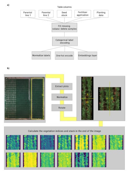
Figure 1.
Scheme of the data processing steps employed for preparing the tabular and spectral datasets as input for the machine learning models. (a) Tabular data processing; categorical feature columns were subjected to the steps listed, they were then normalized, one-hot encoded, or used in embedding layers for testing. (b) Multispectral image processing. The images collected by the UAV were used to build the orthomosaic, the individual maize plots were then extracted, the pixel values were normalized and, finally, the plot was cut and stacked in random order. The vegetation indices were calculated as new spectral bands, and are shown in the image in the following order: blue, green, red, red edge, NIR, NDVI, NDVI-RE, NDRE, ENVI, CCCI, GNDVI, GLI and OSAVI.
The experimental field data included parental lines, seed source (stock), fertilizer application, planting date, and days after sowing, and were processed to be used as training data for the tabular machine learning models. The categorical features were encoded using tab_processing.ipynb that employs the scikit-learn (0.23.2) label encoder for turning categorical features into numerical vectors and one-hot encoders, and the fastai library (v2.1.5) was used for constructing the embedding layer for each feature [33]. The categorical columns, mapped to numerical values, were normalized to fit the range 0–1. There were 5.41% maize plots with missing values from a total of 4487 plots; the majority were filled using the value from their replicate, and 1.18% plots were deleted as the replicate values were also missing. The datasets from 2017, 2018 and 2019 were combined and split into training and holdout sets (90:10). The training dataset was further split into training and validation sets (70:30). The holdout dataset contained data from the three years that were not used during model development but were subject to the same technical and environmental conditions. Results in the holdout dataset in this case indicate the model’s performance for predicting early yield under different environmental conditions.
2.3. Machine Learning Models
2.3.1. Machine Learning Module for Tabular Data
The machine learning modules for yield prediction, based on tabular data, were trained using parental lines, seed source (stock), fertilizer application (optimal or reduced), planting (optimal or late), and the number of days after sowing. Due to the impact of hyperparameters on the performance of machine learning models, the hyperparameters for the random forest, XGBoost, and tabular deep neural network (tab-DNN) were defined after conducting one thousand trials with different hyperparameter combinations, using the Optuna (v2.3) framework. Optuna searches the user-defined hyperparameter space and efficiently discards values with low performance, returning the best hyperparameter set encountered across the trials [34]. For random forest, we searched the minimum sample leaf, the number of estimators and minimal sample split values; XGBoost searched for the optimal learning rate, the number of estimators, maximum depth and minimum child weight; and the DNN searched for the learning rate, optimization function, and the number of layers. Two encoding methods were tested for random forest and XGBoost: ordinal encoding and one-hot-encoding using scikit-learn (0.23.2). The DNN was implemented using fastai v2.1.5 [33] and PyTorch v1.7 [35]. Categorical features were encoded using entity embeddings [36]. Embedding layers learn from the feature distribution in the whole dataset, clustering categorical variables with higher similarity and exposing the intrinsic relationship between them; they are an effective way to map features in an embedding space [36]. The output from the embedding layers was concatenated to the continuous features and was used as input for the DNN (Figure 2). The implementation of the machine learning models for tabular data used tabular_models.ipynb.
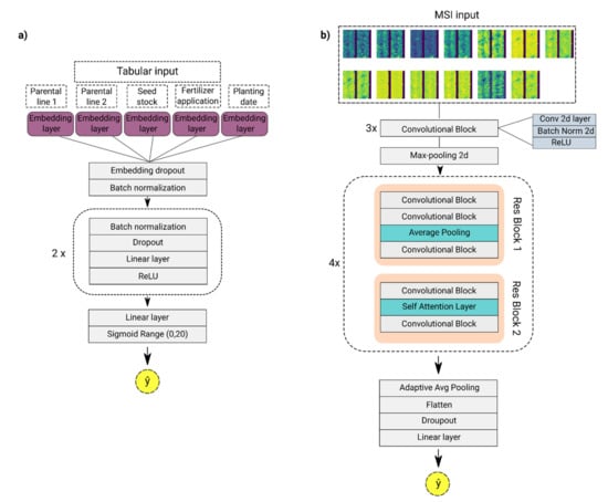
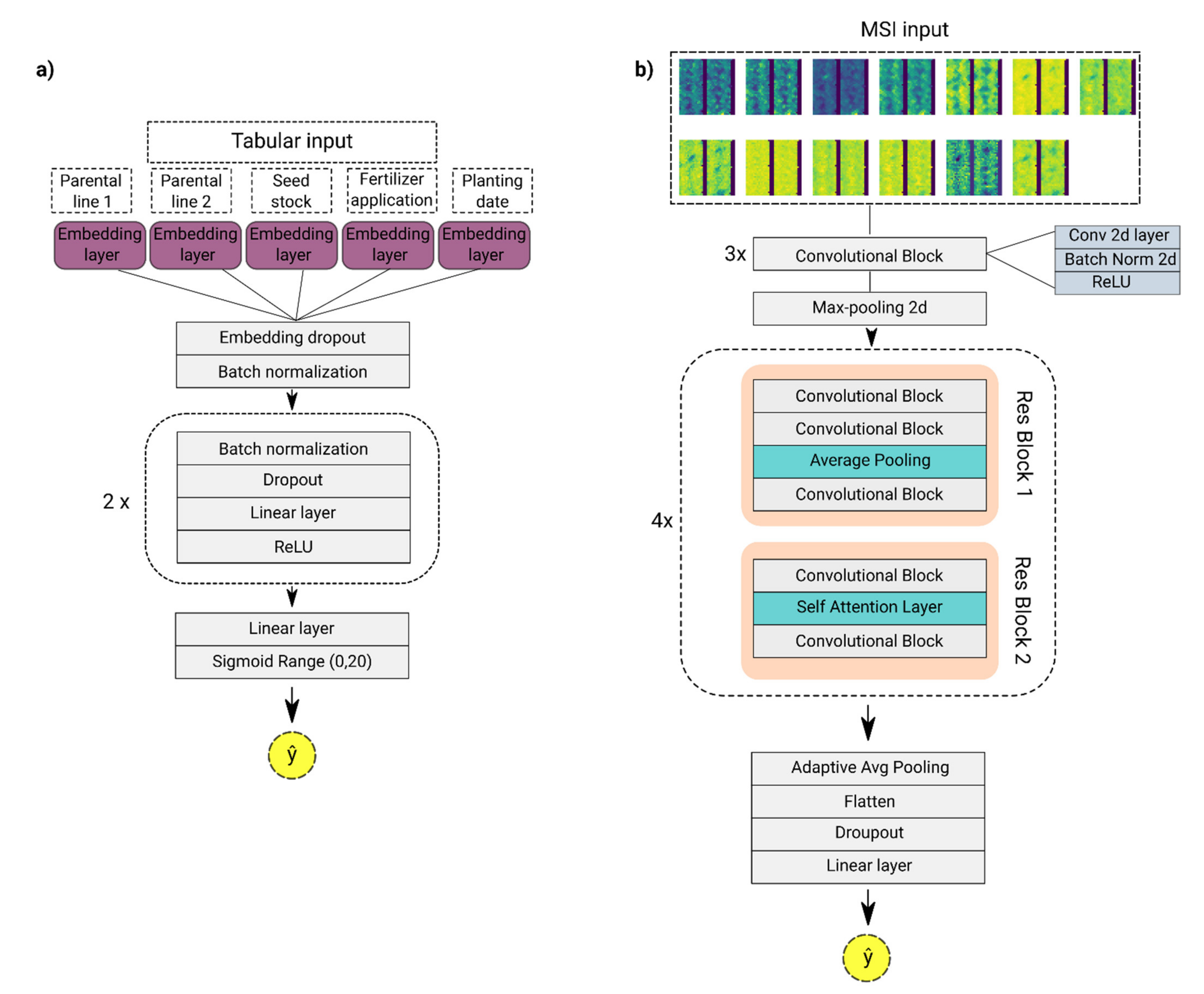
Figure 2.
Schematic representation of the deep learning model architectures; ŷ indicates the yield prediction output by the model. In (a) and (b), some layer blocks are repeated, as indicated by the dotted line. (a) Tab-DNN architecture with embedding layers. The tab-DNN is trained based on genotype and crop management data, as indicated in the image. (b) The sp-DNN architecture is based on a modified resnet18 with a self-attention layer. The sp-DNN was trained with the spectral images plus vegetation indices bands, calculated per pixel. The self-attention layer is present once in the first block repetition, whereas the average pooling layer is not present in the first block iteration.
2.3.2. Deep Learning Module for Multispectral Imagery
The spectral deep neural network (sp-DNN) for yield prediction was trained using the processed multispectral images, plus the calculated vegetation indices bands, resulting in input images with 13 spectral bands. The sp-DNN uses a modified version of the residual neural network architecture with 18 layers (ResNet18) to process the multispectral images. The ResNet architecture employed comprises optimized convolutional layers, and a self-attention layer [37,38]. The self-attention mechanism helps model the relationship between distant regions of the input image, computing an attention weight matrix that indicates the most relevant regions for the prediction [39]. The hyperparameter search library Optuna (v2.3) [34] was used to determine the sp-DNN architecture: the number of layers, activation function, learning rate, and if attention layers were applied. The general model architecture is shown in Figure 2, and the model script is available at msi_model.ipynb.
2.3.3. Multimodal Deep Learning Framework
The multimodal deep learning model was composed of the tab-DNN and sp-DNN modules described in Section 2.3.1. and Section 2.3.2., followed by a fusion module with two linear layers and ReLU as an activation function. The weights from the last layer from tab-DNN and sp-DNN are concatenated and fed as input for the fusion module. Gradient blending was employed to address the calibration of multiple loss functions for the modules [40], with scaling weights depending on how long each module takes to converge (tabular module 0.1, spectral module 0.55, and fusion module 0.35). Scaling the modules helps to prevent overfitting when the modules are trained simultaneously, as different input data and module architectures are likely to converge at different times [40]. Each module outputs its yield prediction, allowing a comparison of performance against the fusion module prediction (Figure 3). Multimodal model performance was compared, using pre-trained modules against training the architecture from scratch with co-learning. The pre-trained multimodal architecture employed previously trained tab-DNN and sp-DNN as modules, with a further 60 epochs of co-training to fine-tune the fusion module, whereas the multimodal architecture was trained from scratch using initialized tab-DNN and sp-DNN modules, and they were trained along with the fusion module. Scripts used for the implementation of this model are multimodal_model.py, multimodal_utils.py, and multimodal_model.ipynb.
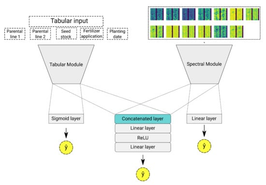
Figure 3.
Scheme showing the multimodal model architecture. The tab-DNN and sp-DNN models output an independent yield prediction value (ŷ) based on their respective input datasets. The weights from the last layer of the tab-DNN and sp-DNN are combined to feed the fusion module, which outputs the multimodal yield prediction (ŷ).
2.4. Evaluation Metrics
Model performance was evaluated using fivefold stratified cross-validation (scikit-learn, 0.23.2). The stratification was performed by year, to ensure that the training and validations datasets were balanced. In stratified cross-validation, the dataset is split between training and validation sets for N consecutive folds, each fold having an equal proportion of samples from the three years. One fold is used once as validation, while the remaining four folds are used for training; this step is repeated until each fold was used as validation once. The metrics employed to measure performance were R2 (coefficient of determination), root mean squared error (RMSE) and relative RMSE (RMSE %), using the following equations:
where y and ŷ are the observed and predicted yield, respectively, for each sample i, and the total number of samples is indicated by n, whereas ymax–ymin are used to indicate the range of observed yield, and ȳ represents the mean of the observed data. The contribution of the VIs to the multimodal prediction performance was assessed using permutation importance, in which the position of the pixels are randomized in the selected VI, breaking the structured association between the feature and prediction [41,42,43]. To measure the VI importance, we compared the difference in performance on RMSE and R2, between the prediction with the randomized VI and the intact VI. A custom python script was used to perform feature assessment: permutation_nb.ipynb.
3. Results
3.1. Maize Grain Yield Distribution
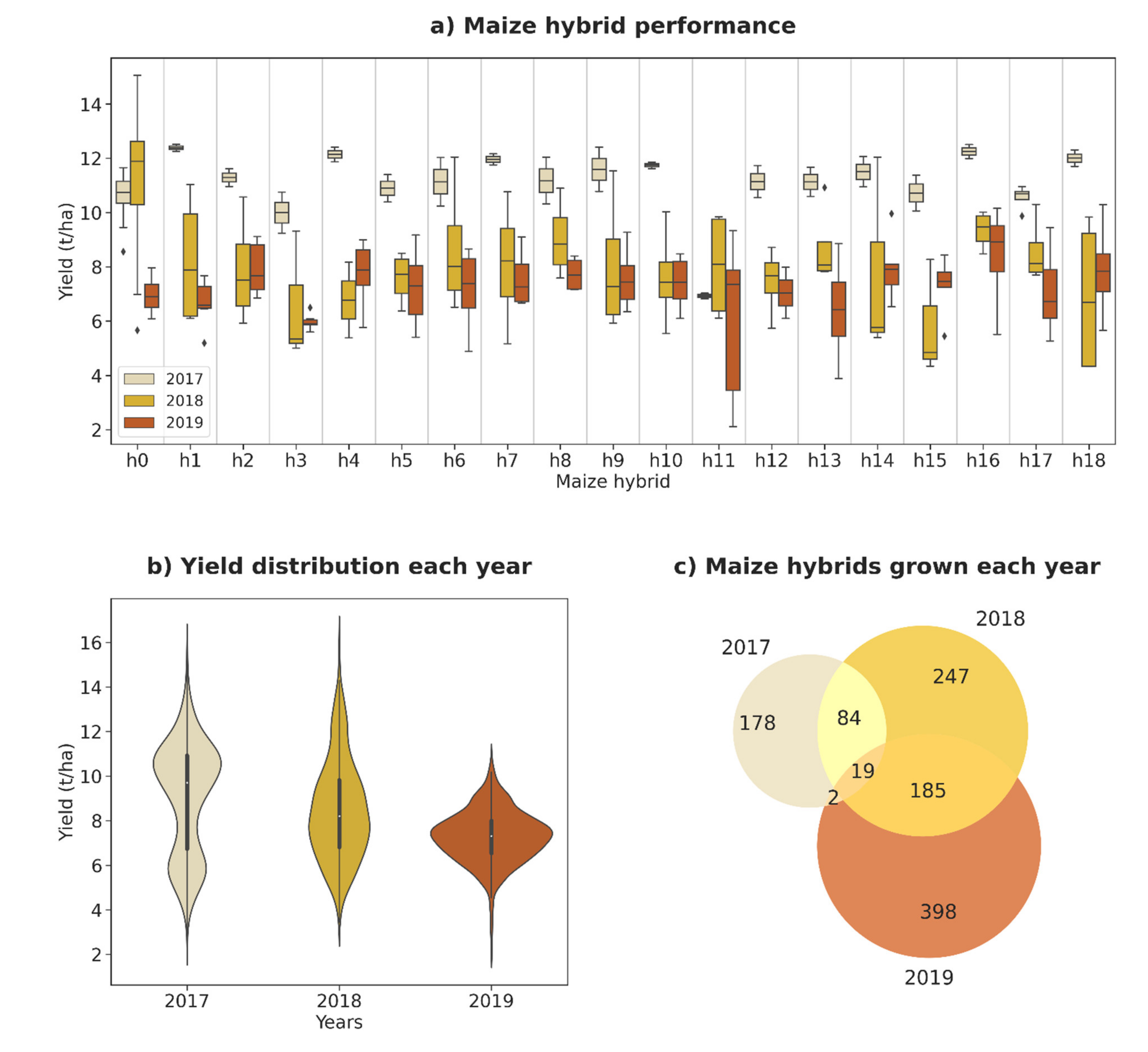
Harvested yield distribution varied across years due to the different seasonal growing conditions. The impact of environmental conditions in each year can be estimated by comparing the performance of nineteen check varieties grown across the three years, under optimal fertilization and planting date conditions (Figure 4a), where the plants grown in 2017 have a higher overall performance than plants grown in the other years. The 2017 trial presents two discernible groups with mean yield values of 10 and 6 t/ha−1, composed of hybrids subjected to P1F1 and P2F1 treatments (Figure 4b). In the 2019 trial, all hybrids were subjected to P1F1 and displayed a consistently low yield compared to previous years, with values ranging from 2 to 11 t/ha−1 although the majority of the plots yielded between 6 to 9 t/ha−1 (Supplementary File S1). In total, 1113 maize hybrid lines were sown from a combination of 1040 unique parent lines (Figure 4c). The under-representation of some parental lines may decrease the accuracy of yield prediction for these hybrids, as there will be a smaller dataset to learn from.

Figure 4.
(a) Comparison of the yield distribution of the same maize hybrids grown each year of the field trial; (b) maize yield distribution per year; (c) number of novel and overlapping maize lines grown each year.
3.2. Machine Learning Hyperparameter Optimization
For the random forest model, the minimum sample leaf was the most important hyperparameter, with 0.91 importance, followed by the number of estimators that define the size of the estimator forest. The optimal number of estimators can vary widely depending on the dataset employed, usually achieving a threshold beyond which there is no increase in accuracy that can justify the computational cost [44]. For XGBoost, the learning rate had the most impact on model performance, with 0.75 importance, followed by the number of estimators. Random forest and XGBoost-optimized model hyperparameters are available in the script tabular_models.ipynb. The tab-DNN and sp-DNN had the same hyperparameter importance order, with the learning rate as the most influential hyperparameter, followed by the optimization function, the number of layers, and the attention layer. The optimized tab-DNN model was composed of a 100-layer network, with ReLU as the activation function, RMSE as the loss function, ranger as the optimization function, a learning rate of 1e-3, batch normalization, dropout (0.5), and an embeddings dropout (0.5). The selection of the optimization function and the number of layers was more relevant to the sp-DNN. The sp-DNN was composed of a ResNet with 18 layers, a self-attention layer, a learning rate of 1e-3, and using Adam as the optimizer [45]. A hyperparameter importance plot is available in Supplementary File S2.
3.3. Prediction of Yield Based on Crop Metadata
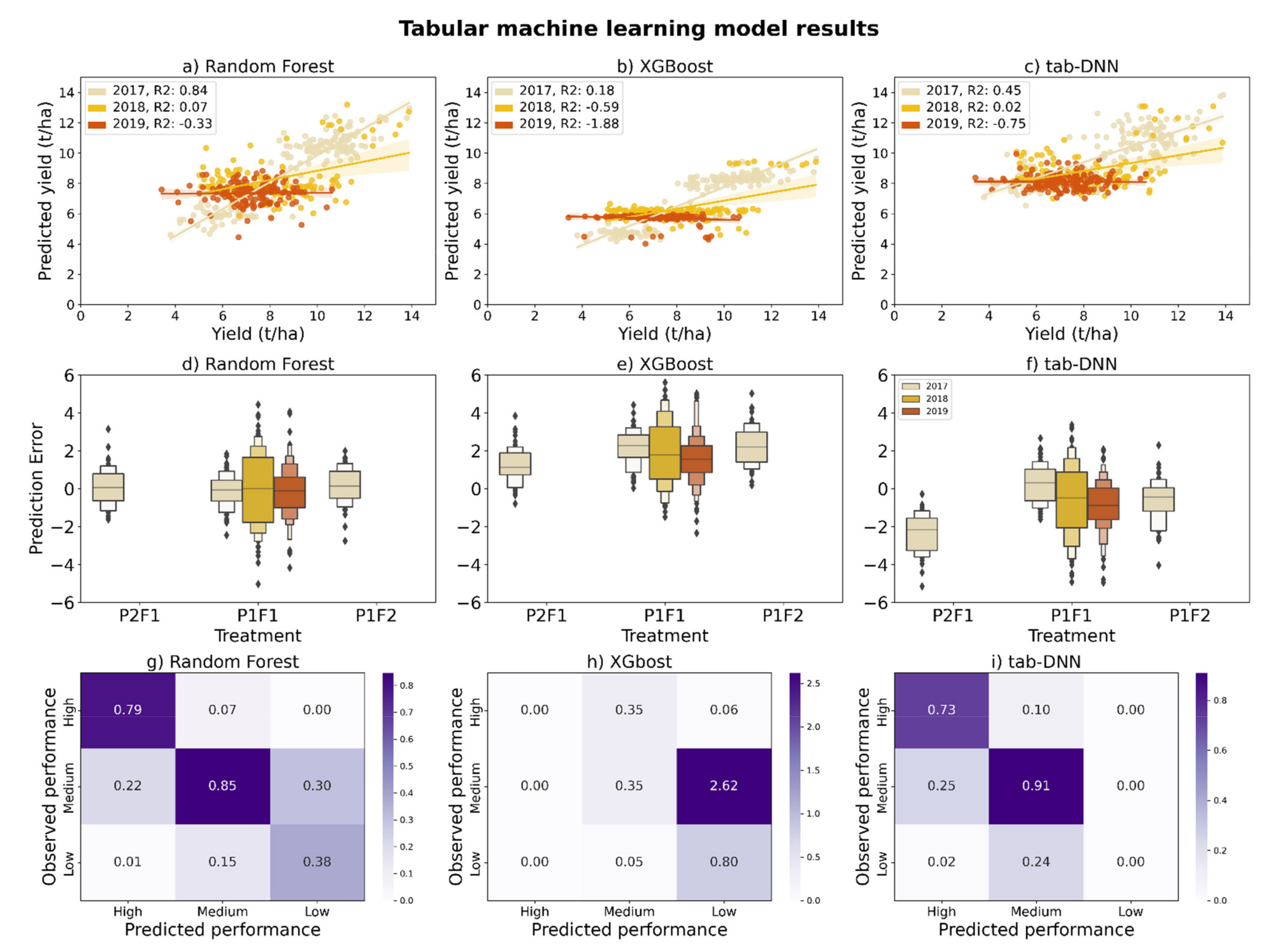
Random forest demonstrated the best overall performance for predicting grain yield based on the genotype and crop management data, followed by the tab-DNN (Table 2). The machine learning models presented between 0.11–0.27% of relative RMSE variation when predicting yield in the validation and holdout datasets, suggesting that the models were not overfitting the training dataset and performed similarly on unseen data. The three models presented a lower R2 score when predicting the yield from the 2019 hybrids. The categorical feature-encoding method had little effect on the prediction accuracy of the validation and holdout sets, with one-hot encoding causing no improvement in the random forest or XGBoost performance. In addition, training the models with one-hot encoded data took longer, as was also observed in a previous study [46]. The range of the predicted grain yield is often more narrow than the actual yield distribution (Figure 5; Supplementary File S3). Although the year feature was hidden from the models, we can observe that random forest and the tab-DNN presented higher error rates for predicting the 2018 and 2019 yields. XGBoost performed worse than other models, grouping hybrids into clusters and providing a single yield value per group, as shown in Figure 5. To assess the capacity of the models to identify high-performance hybrids, each plot was placed into categories based on their performance and labeled as high- (above 10 t/ha), medium- (between 6 and 9.99 t/ha), and low-yield plots (below 6 t/ha). Sorting the hybrids into categories showed that random forest and tab-DNN were able to identify approximately 76% of the high-performance hybrids, but were incapable to identify more than 38% of the low-performance plots (Figure 5G–I).
Table 2.
Performance comparison of different machine learning models, using fivefold cross-validation. Values are presented with their standard variation. The best model’s result is highlighted in bold.
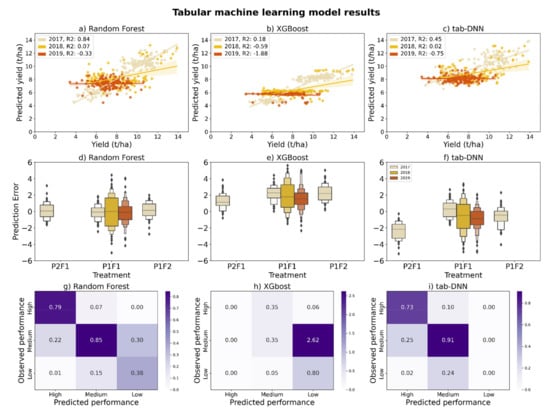
Figure 5.
Machine learning model predictions of hybrid yield on the holdout dataset (2017—2019) based on genotype and crop management data. (a–c) show the predicted yield (t/ha) in the y-axis in comparison to the ground-truth yield (t/ha) in the x-axis for each sample in the holdout dataset. (d–f) present the model prediction error per treatment, the error value was obtained by subtracting the predicted yield from harvested yield. (g–i) show the percentage of hybrid plots classified as high, medium and low yield. The x-axis shows the predicted labels, and the y-axis is the ground-truth label.
3.4. Spectral Feature Deep Learning Model Performance
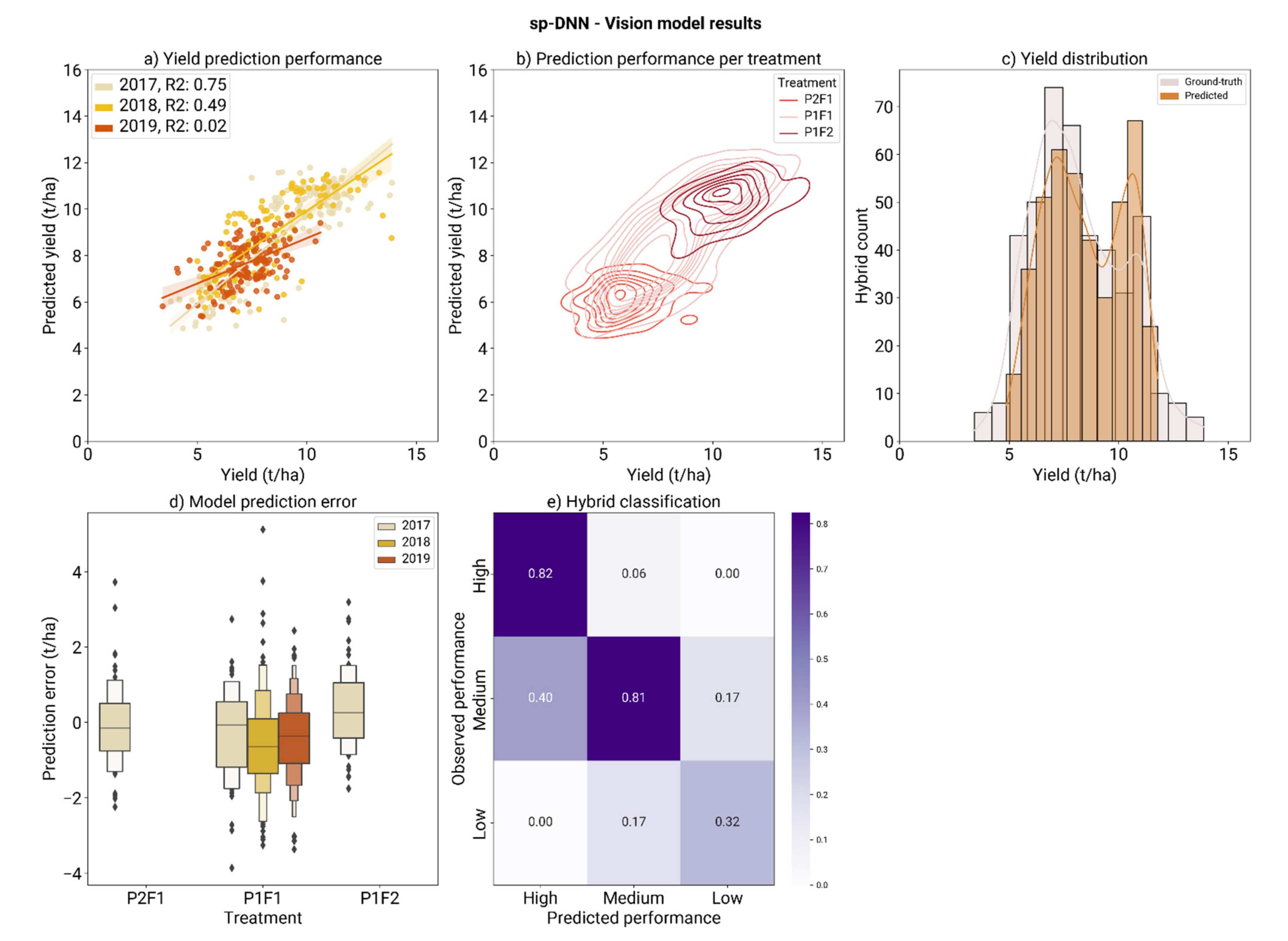
The sp-DNN was trained using thirteen spectral bands, including the eight calculated VIs. The trained model predicted grain yield with 8.99% relative RMSE in the holdout dataset, as shown in Table 3. The model predictions accurately reflect the treatment groupings P1F2 and P2F1, with no changes in the image capture and reflectance calibration. The capacity of the model to group P1F2 and P2F1 predictions shows that the spectral features were indicative of the plant conditions. In addition, the bimodal tendency observed in the ground-truth yield is accentuated in the predicted yield (Figure 6). The model R2 score was higher for the prediction of 2017 and 2018 hybrids, although 2017 presented a significantly higher error rate than other years (p-value > 0.05), but no significant difference in prediction error was observed between most treatments except for P1F1, compared to P1F2. The sp-DNN model successfully identified the majority of high-yielding varieties (above 10 t/ha), surpassing the tabular machine learning models and tab-DNN (Figure 6E).
Table 3.
Yield prediction performance of sp-DNN using multispectral features. The validation dataset values were obtained through fivefold cross-validation and presented with standard deviation.

Figure 6.
Sp-DNN yield predictions for the holdout dataset. (a) Comparison of the predicted yield (t/ha) to ground-truth yield (t/ha); (b) visualization of the model predictions, colored by treatment; (c) distribution of maize hybrids by predicted and ground-truth yield (t/ha); (d) prediction error (t/ha) of each treatment colored by year; (e) percentage of high, medium and low-yielding plots, classified as such by the model; the ground-truth plot label is indicated in the y-axis and predicted labels in the x-axis.
3.5. Multimodal Deep Learning Model Performance
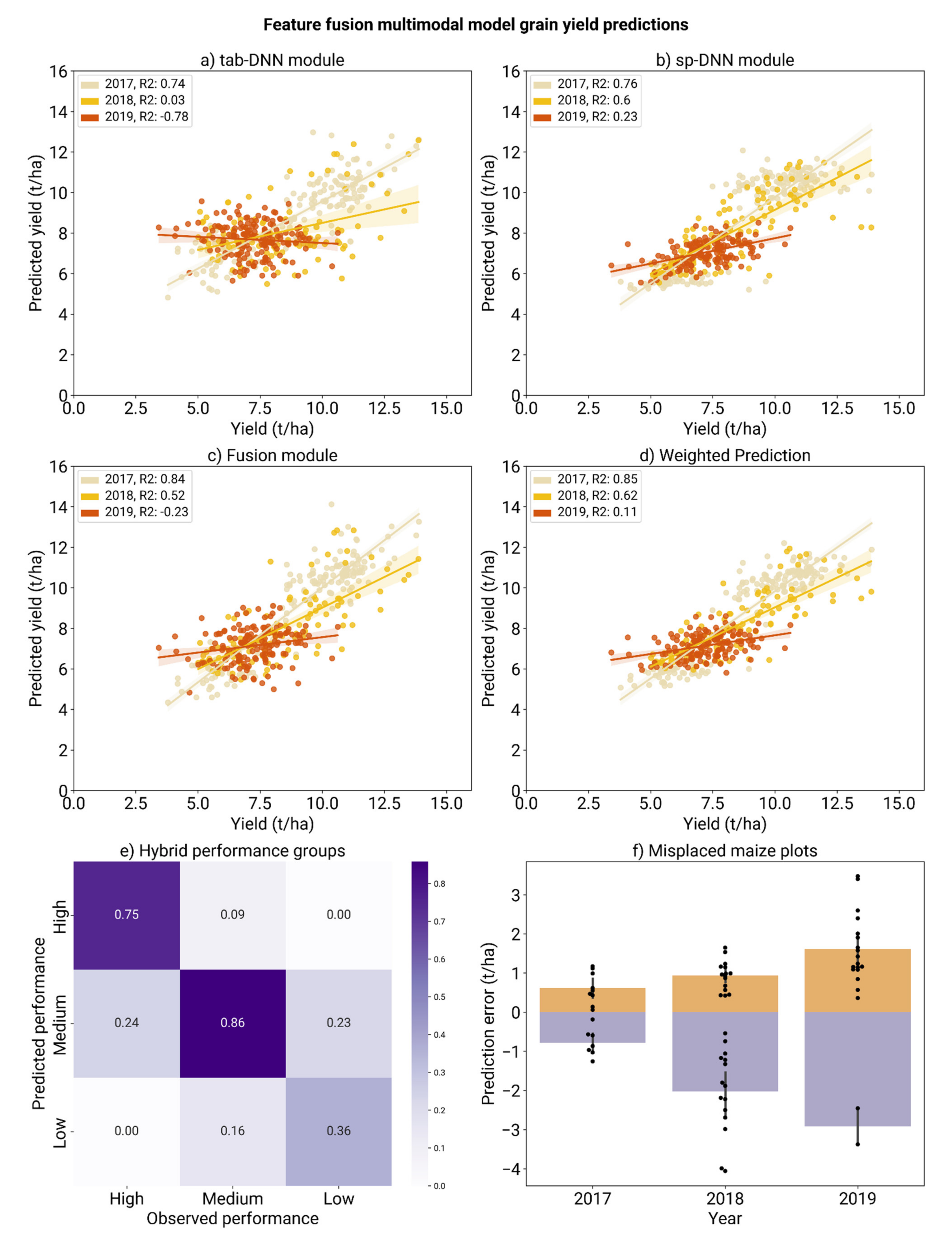
Multimodal co-learning enables sharing complementary information from different modalities, influencing model performance even if one of the modalities is absent during test and validation [25]. In our case, we used co-learning to train the modules and used the weights to feed the fusion module. In this framework, each module outputs an individual prediction, based solely on its data type, being completely independent of the sister modality used during training. Co-learning improved the performance of both modules, as shown in Table 4. The tab-DNN module benefitted substantially and increased the correlation of the prediction in the holdout dataset from 0.27 R2 when trained independently to 0.47 R2 under the co-learning scheme. The greatest prediction performance was obtained by scaling the predictions of the tabular, spectral and fusion modules, using the weights defined during training (0.5, 0.35, 0.6), achieving 7.60% of relative RMSE (equivalent to 1.22 t/ha−1 RMSE) in the holdout dataset, and around 8% of relative RMSE in the validation dataset. No significant difference in performance was observed using pre-trained modules or training them from scratch, there was also no significant difference in the error rate of predictions for plots grown under any treatment or year (p > 0.05).
Table 4.
Performance comparison of multimodal models with late feature fusion. Validation dataset results were obtained with fivefold cross-validation and presented with standard deviation. The weighted prediction was obtained by scaling each module’s prediction and summing the predicted yield. The best-performing models are highlighted in bold.
The maize plots were placed into categories based on their performance, labeled as high- (above 10 t/ha), medium- (between 6 and 9.99 t/ha), and low-yield plots (below 6 t/ha). Sorting the hybrids into categories showed that the multimodal model was able to identify around 75–86% of the high- and medium-performance hybrid plots and 36% of the low-performance plots, which is expected due to the low RMSE (Figure 7). Further investigation suggests that the majority of underestimated plots were from 2017, whereas 2019 had the most plots expected to perform better than they did. Comparing the prediction error of hybrids sown on multiple years or their replicates shows a small prediction error (Supplementary File S3).
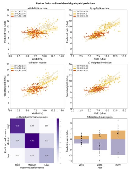
Figure 7.
Images (a–d) shows the multimodal fusion model prediction of grain yield (t/ha) from each module and the weighted prediction. Each module prediction is based on their specific data modality, whereas the weighted prediction is obtained by scaling each module’s prediction and summing the predicted yield. Image (e) shows the model prediction of each maize plot as high-, medium- and low-yield plots (in the y axis), comparing their ground-truth yield in the x-axis. The values within the square indicate the percentage of each category that were predicted to be high-, medium- and low-yield plots. Image (f) shows the optimization error of maize plots that presented a high yield but were predicted as medium (in light purple), and plots with a low yield that were predicted to have medium performance (mustard). The plots are separated by year.
3.6. Effect of Spectral Features on the Prediction of End-of-Season Traits
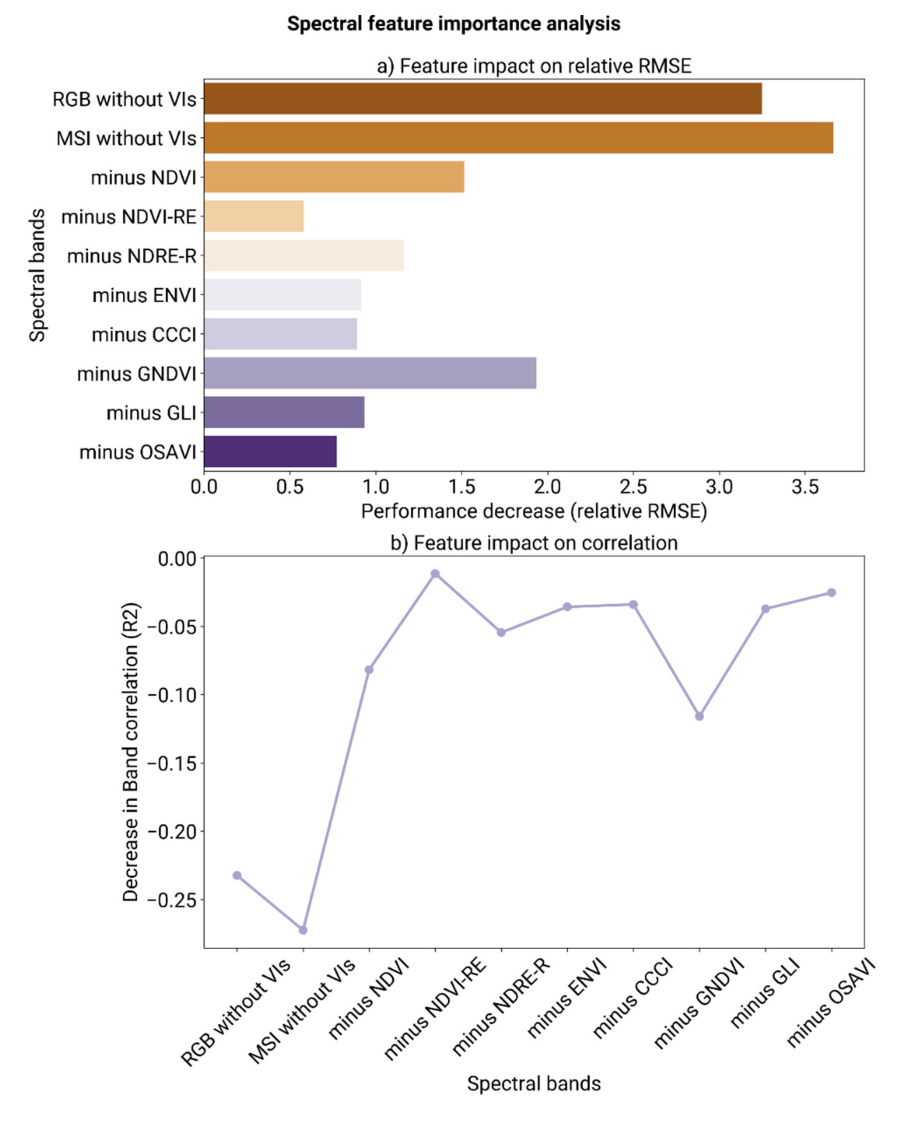
The impact of different VIs in the multimodal model predictions was measured using feature permutation. The performance of the multimodal model was negatively affected by removing the VI bands as shown in Figure 8. Removing all proposed VIs increased the relative RMSE from 7.60%, obtained with the complete dataset, to 10.84%. The correlation between spectral features and grain yield also decreased substantially from 0.72 to 0.45 R2. GNDVI and NDVI were the most influential VIs, with the randomization of the values causing the most impact on the model performance and feature correlation to grain yield prediction. The other VIs had a minor effect on the performance, and the absence of either of them decreased the accuracy of prediction. There was little difference between the prediction performance using RGB- or MSI-only images; however, the majority of VIs used the red edge or near-infrared bands, which may influence the decision to employ a multispectral sensor instead of RGB.
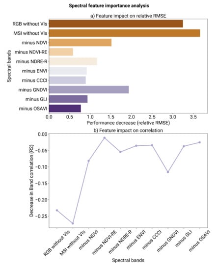
Figure 8.
Prediction results from the permutation analysis. Image (a) shows the impact of randomization on model performance, the x-axis indicates if all VIs were randomized (MSI or RGB) or if only one VI was randomized (minus VI); the y-axis indicates the relative RMSE obtained. Image (b) shows the impact of feature randomization on the correlation between features and grain yield. MSI refers to the original multispectral bands (red, green, blue, near-infrared and red edge).
4. Discussion
Plant selection at an early stage is challenging due to the impact of weather variability and the time needed for the plant to show discernible traits; however, studies in maize and soybean crops have shown that early phenotypic traits, collected with HTP platforms, can be used as an indicator of yield under optimal conditions [47,48]. In maize, a previous study using the 2017 G2F dataset identified loci associated with controlling plant height at early development, which showed a significant impact on yield prediction [48]. In our study, the use of early phenotypic data and genotype showed varied results, depending on the machine learning model employed, with the multimodal model presenting a higher prediction accuracy. Assessing the tabular machine learning models independently, Random forest outperformed XGBoost and tab-DNN in this dataset, indicating its effectiveness for crop yield prediction using a single type of data. The random forest method has been extensively applied for crop yield prediction [4,49,50,51,52,53], with previous studies showing it to outperform other machine learning algorithms in selected datasets [50,53]. XGBoost had the worst performance among the machine learning models tested, placing the samples into yield groups. This behavior suggests that the tabular dataset had an insufficient number of features for XGBoost to separate low and high-yielding hybrids, as previous studies showed XGBoost as competent when dealing with larger datasets [54,55]. Tab-DNN was selected as a module for the multimodal architecture, due to its potential for improvement within the co-learning framework. When independently trained using the tabular dataset, tab-DNN showed a higher error rate for the P1F1 treatment, which included samples grown in the three years without the data year being indicted in any feature, which may have caused the seasonal variability to impact prediction accuracy. In P2F1, the yield was consistently lower than other treatments because the hybrids were sown later in the season and experienced heat stress. A study using the same dataset hypothesized that delayed planting in that region of Texas, US, may increase photosynthetic activity, leading to increased plant height and lower yield [48].
Regarding the sp-DNN module, the bimodal tendency observed in the ground-truth yield data is accentuated in the predicted yield (Figure 6), with a larger number of plots being predicted to have a higher yield. The sp-DNN module trained with spectral data from the crop’s early stages presented a higher prediction accuracy with R2 0.63 than the machine learning algorithms based on genotype and crop management (R2 0.53). Several factors may have contributed to this result, as the spectral features are capable of indicating the plant’s health status and biomass coverage [56,57]. Both tab-DNN and sp-DNN modules showed a tendency for more conservative predictions toward the mean, predicting a narrower yield range than ground-truth data.
The multimodal model was able to predict yield across three consecutive years, with a relative RMSE of 7.6% and R2 of 0.73. The modules consistently presented a low R2 score for the early yield prediction of 2019 hybrids; this may be due to the parental lines presenting a different performance in previous years, which may introduce a bias to the model. It outperformed previous models based on spectral features for early yield prediction, for both soybean (an RMSE of 9.82 and R2 of 0.68) [3] and maize subjected to phosphorus treatments (R2 between 0.15~0.82) [58]. The higher accuracy may be due to the capacity of multimodal deep learning to incorporate different data into the prediction. Multimodal deep learning models have been used for crop yield prediction using spectral features from later development stages, where plant growth has a higher correlation with the final yield. Nonetheless, our model had comparable performance, with two multimodal models for soybean yield prediction using images from plant reproductive stages (a relative RMSE of 15.9% and R2 of 0.72) [29], and for cotton-yield prediction using images from flowering and shortly before harvest (a relative RMSE of 6.8% and R2 of 0.94) [59]. Multimodality deep learning models can support early yield prediction, due to the complementary information shared within the model [25]. Training the spectral and tabular features together has improved both module predictions, increasing tab-DNN performance on the holdout from R2 0.27 to 0.47, and the sp-DNN R2 from 0.63 to 0.71 in the holdout dataset. The improvement in accuracy caused by multimodal data is corroborated by previous studies; it was reported that adding spectral features improved the prediction of grain yield in wheat by 70% [5], and in maize, it increased by 0.1 in R2 [60]. Here, we demonstrate that a model using two types of input data shows higher accuracy compared to single-data models, one that is valuable when trained using data from young plants with few measurements to inform the model. The multimodal model presented here showed high accuracy (relative RMSE 7.6%) for early yield prediction, being suitable as a decision support tool that can inform breeders of the most productive hybrids. However, it is important to notice that using the model for early yield prediction of another species or under different treatment may require fine-tuning, using the current model as a base for transfer learning [61]. Further training of the model can be achieved by using private or other publicly available datasets [62]. In addition, the multimodal framework can be expanded with the inclusion of new specialized modules for weather, soil and other sensor data, as previous studies show their impact on model accuracy [17,63,64].
Identifying the components that lead to deep learning model prediction is a useful step in verifying model coherence, reducing noise, and improving the overall model [65]. The contribution of the spectral components for the model prediction can be used to extract insights, as the spectral features can capture different aspects of the plant phenotype. In this study, VIs had a high impact on the prediction, causing a substantial decrease in model performance when using RGB or multispectral images alone. RGB images performed better than using multispectral images alone, which was also observed in another study assessing the early growth of maize hybrids under phosphorus treatments [58]. However, the majority of VIs employed the red edge or near-infrared bands, which may influence the decision toward collecting the raw data, using a multispectral sensor instead of RGB. Our observation of the importance of NDVI and GNDVI to predict crop traits is similar to previous studies using VIs. For example, a study using 33 different VIs reported that NDVI, NDRE and GNDVI had the strongest correlation with maize yield [49]. Other studies also demonstrate NDVI correlation with grain yield and moisture, suggesting its use as a secondary trait for plant selection during trials [58,66,67]. For wheat, NDVI provided spatial separation between the high- and low-yielding regions within a plot during the anthesis, tillering, and seedling stages [68]. NDVI and GNDVI are usually related to biomass and tend to saturate at later growth stages [57]. However, since the aim was to predict yield at an early stage, including NDVI and GNDVI was advantageous. Contrary to previous studies, OSAVI only had a minor contribution to yield prediction at an early stage, even though this index is commonly employed for prediction in sparse vegetation as it corrects soil interference in the reflectance [69,70]. The minor effect of OSAVI and other VIs may be explained due to redundancy in the information provided by the other indices, which may partially compensate for the absence of one or another VI. Nonetheless, even OSAVI and other low-contributing VIs increased the model performance to some extent, and it is advantageous to include them in the training data.
5. Conclusions
Early selection of the highest performing crop plants in a field trial can accelerate breeding, reducing the cost and duration of the breeding cycle. Here, we demonstrate a clear advantage of using multiple data types for early yield prediction, and how training specialized modules together can help improve prediction accuracy. Although previous studies have shown that adding extracted spectral features can improve genotype selection accuracy, using a multimodal deep learning algorithm was not previously explored. The multimodal model developed in this study achieved high performance for early yield prediction and could provide a decision support tool for breeders. However, it is important to notice that it was trained using single-location data, and it would require further training with new datasets to be applicable to different locations. In addition, the model accuracy can be improved by regularly updating the model after each season, as the new data can show variation in the hybrids’ performance or integrate new hybrids into the training set. This approach is commonly used in machine learning to ensure that the training dataset does not deviate much from the target dataset we are trying to predict. Further research could explore whether the inclusion of other data types such as weather, soil and genetic information can contribute to improving model accuracy, as they play an important role in plant performance.
Supplementary Materials
The following are available online at https://www.mdpi.com/article/10.3390/rs13193976/s1: Supplementary file S1: Maize distribution of observed yield separated per year. Supplementary file S2: Hyperparameter importance analysis from each of the machine and deep learning models optimized; Supplementary file S3: Distribution of the yield prediction from tabular machine learning models in comparison to the actual yield distribution, indicating how the model predictions fit the actual yield data; Supplementary file S4: Prediction error (t/ha) of each hybrid and its replicate across different years and treatments in the holdout dataset.
Author Contributions
M.F.D. analyzed the data, developed the model and wrote the manuscript; P.E.B., F.B., M.B. and D.E. provided additional analysis and data interpretation and edited the manuscript. All authors have read and agreed to the published version of the manuscript.
Funding
The Australian Government supported this work through the Australian Research Council (Projects DP210100296 and DP200100762) and the Grains Research and Development Corporation (Projects 9177539 and 9177591). Monica F. Danilevicz was supported by the Research Training Program scholarship and the Forrest Research Foundation.
Data Availability Statement
The dataset used in this study was kindly made available by the Genomes to Fields initiative (www.genomes2fields.org, accessed 25 March 2021) at doi: 10.25739/4ext-5e97, 10.25739/96zv-7164 and 10.25739/d9gt-hv94 accessed 25 March 2021. The code used for the analysis and model development is available at https://github.com/mdanilevicz/maize_early_yield_prediction.git, accessed 16 August 2021.
Acknowledgments
We would like to thank Seth Murray and his group for releasing the data used in this study and welcoming our inquiries about the datasets. We would also like to thank the Pawsey Supercomputing Centre for computation resources.
Conflicts of Interest
The authors declare no conflict of interest.
References
- Challinor, A.J.; Koehler, A.K.; Ramirez-Villegas, J.; Whitfield, S.; Das, B. Current Warming Will Reduce Yields Unless Maize Breeding and Seed Systems Adapt Immediately. Nat. Clim. Chang. 2016, 6, 954–958. [Google Scholar] [CrossRef]
- Bai, G.; Ge, Y.; Hussain, W.; Baenziger, P.S.; Graef, G. A Multi-Sensor System for High Throughput Field Phenotyping in Soybean and Wheat Breeding. Comput. Electron. Agric. 2016, 128, 181–192. [Google Scholar] [CrossRef] [Green Version]
- Yuan, W.; Wijewardane, N.K.; Jenkins, S.; Bai, G.; Ge, Y.; Graef, G.L. Early Prediction of Soybean Traits through Color and Texture Features of Canopy RGB Imagery. Sci. Rep. 2019, 9, 14089. [Google Scholar] [CrossRef] [PubMed] [Green Version]
- Varela, S.; Pederson, T.; Bernacchi, C.J.; Leakey, A.D.B. Understanding Growth Dynamics and Yield Prediction of Sorghum Using High Temporal Resolution UAV Imagery Time Series and Machine Learning. Remote Sens. 2021, 13, 1763. [Google Scholar] [CrossRef]
- Rutkoski, J.; Poland, J.; Mondal, S.; Autrique, E.; Pérez, L.G.; Crossa, J.; Reynolds, M.; Singh, R. Canopy Temperature and Vegetation Indices from High-Throughput Phenotyping Improve Accuracy of Pedigree and Genomic Selection for Grain Yield in Wheat. G3 (Bethesda) 2016, 6, 2799–2808. [Google Scholar] [CrossRef] [PubMed] [Green Version]
- Zhang, L.; Niu, Y.; Zhang, H.; Han, W.; Li, G.; Tang, J.; Peng, X. Maize Canopy Temperature Extracted from UAV Thermal and RGB Imagery and Its Application in Water Stress Monitoring. Front. Plant Sci. 2019, 10, 1270. [Google Scholar] [CrossRef]
- Ihuoma, S.O.; Madramootoo, C.A. Sensitivity of Spectral Vegetation Indices for Monitoring Water Stress in Tomato Plants. Comput. Electron. Agric. 2019, 163, 104860. [Google Scholar] [CrossRef]
- Al-Saddik, H.; Simon, J.-C.; Cointault, F. Development of Spectral Disease Indices for “flavescence Dorée” Grapevine Disease Identification. Sensors 2017, 17, 2772. [Google Scholar] [CrossRef] [Green Version]
- Zhang, M.; Qin, Z.; Liu, X.; Ustin, S.L. Detection of Stress in Tomatoes Induced by Late Blight Disease in California, USA, Using Hyperspectral Remote Sensing. Int. J. Appl. Earth Obs. Geoinf. 2003, 4, 295–310. [Google Scholar] [CrossRef]
- Mutka, A.M.; Bart, R.S. Image-Based Phenotyping of Plant Disease Symptoms. Front. Plant Sci. 2014, 5, 734. [Google Scholar] [CrossRef] [Green Version]
- Zhao, H.; Yang, C.; Guo, W.; Zhang, L.; Zhang, D. Automatic Estimation of Crop Disease Severity Levels Based on Vegetation Index Normalization. Remote Sens. 2020, 12, 1930. [Google Scholar] [CrossRef]
- Wilke, N.; Siegmann, B.; Frimpong, F.; Muller, O.; Klingbeil, L.; Rascher, U. Quantifying Lodging Percentage, Lodging Development and Lodging Severity Using a Uav-Based Canopy Height Model. Int. Arch. Photogramm. Remote Sens. Spatial Inf. Sci. 2019, XLII-2/W13, 649–655. [Google Scholar] [CrossRef] [Green Version]
- Chu, T.; Starek, M.J.; Brewer, M.J.; Masiane, T.; Murray, S.C. UAS Imaging for Automated Crop Lodging Detection: A Case Study over an Experimental Maize Field. In Autonomous Air and Ground Sensing Systems for Agricultural Optimization and Phenotyping II; Thomasson, J.A., McKee, M., Moorhead, R.J., Eds.; SPIE: Washington, DC, USA, 2017; Volume 10218, p. 102180. [Google Scholar]
- LeCun, Y.; Bengio, Y.; Hinton, G. Deep Learning. Nature 2015, 521, 436–444. [Google Scholar] [CrossRef]
- Schmidhuber, J. Deep Learning in Neural Networks: An Overview. Neural Netw. 2015, 61, 85–117. [Google Scholar] [CrossRef] [PubMed] [Green Version]
- Van Klompenburg, T.; Kassahun, A.; Catal, C. Crop Yield Prediction Using Machine Learning: A Systematic Literature Review. Comput. Electron. Agric. 2020, 177, 105709. [Google Scholar] [CrossRef]
- Khaki, S.; Wang, L.; Archontoulis, S.V. A CNN-RNN Framework for Crop Yield Prediction. Front. Plant Sci. 2019, 10, 1750. [Google Scholar] [CrossRef] [PubMed]
- Sun, J.; Di, L.; Sun, Z.; Shen, Y.; Lai, Z. County-Level Soybean Yield Prediction Using Deep CNN-LSTM Model. Sensors 2019, 19. [Google Scholar] [CrossRef] [PubMed] [Green Version]
- Nevavuori, P.; Narra, N.; Linna, P.; Lipping, T. Crop Yield Prediction Using Multitemporal UAV Data and Spatio-Temporal Deep Learning Models. Remote Sens. 2020, 12, 4000. [Google Scholar] [CrossRef]
- Terliksiz, A.S.; Altylar, D.T. Use of Deep Neural Networks for Crop Yield Prediction: A Case Study of Soybean Yield in Lauderdale County, Alabama, USA. In Proceedings of the 2019 8th International Conference on Agro-Geoinformatics (Agro-Geoinformatics), Instanbul, Turkey, 16 July 2019; IEEE; pp. 1–4. [Google Scholar]
- Khaki, S.; Pham, H.; Wang, L. Simultaneous Corn and Soybean Yield Prediction from Remote Sensing Data Using Deep Transfer Learning. Sci. Rep. 2021, 11, 11132. [Google Scholar] [CrossRef]
- Nevavuori, P.; Narra, N.; Lipping, T. Crop Yield Prediction with Deep Convolutional Neural Networks. Comput. Electron. Agric. 2019, 163, 104859. [Google Scholar] [CrossRef]
- Maimaitijiang, M.; Ghulam, A.; Sidike, P.; Hartling, S.; Maimaitiyiming, M.; Peterson, K.; Shavers, E.; Fishman, J.; Peterson, J.; Kadam, S.; et al. Unmanned Aerial System (UAS)-Based Phenotyping of Soybean Using Multi-Sensor Data Fusion and Extreme Learning Machine. ISPRS J. Photogramm. Remote Sens. 2017, 134, 43–58. [Google Scholar] [CrossRef]
- Herrero-Huerta, M.; Rodriguez-Gonzalvez, P.; Rainey, K.M. Yield Prediction by Machine Learning from UAS-Based Mulit-Sensor Data Fusion in Soybean. Plant Methods 2020, 16, 78. [Google Scholar] [CrossRef]
- Baltrusaitis, T.; Ahuja, C.; Morency, L.-P. Multimodal Machine Learning: A Survey and Taxonomy. IEEE Trans. Pattern Anal. Mach. Intell. 2019, 41, 423–443. [Google Scholar] [CrossRef] [PubMed] [Green Version]
- Gao, J.; Li, P.; Chen, Z.; Zhang, J. A Survey on Deep Learning for Multimodal Data Fusion. Neural Comput. 2020, 32, 829–864. [Google Scholar] [CrossRef] [PubMed]
- Khaki, S.; Khalilzadeh, Z.; Wang, L. Classification of Crop Tolerance to Heat and Drought—A Deep Convolutional Neural Networks Approach. Agronomy 2019, 9, 833. [Google Scholar] [CrossRef] [Green Version]
- Pantazi, X.E.; Moshou, D.; Alexandridis, T.; Whetton, R.L.; Mouazen, A.M. Wheat Yield Prediction Using Machine Learning and Advanced Sensing Techniques. Comput. Electron. Agric. 2016, 121, 57–65. [Google Scholar] [CrossRef]
- Maimaitijiang, M.; Sagan, V.; Sidike, P.; Hartling, S.; Esposito, F.; Fritschi, F.B. Soybean Yield Prediction from UAV Using Multimodal Data Fusion and Deep Learning. Remote Sens. Environ. 2020, 237, 111599. [Google Scholar] [CrossRef]
- McFarland, B.A.; AlKhalifah, N.; Bohn, M.; Bubert, J.; Buckler, E.S.; Ciampitti, I.; Edwards, J.; Ertl, D.; Gage, J.L.; Falcon, C.M.; et al. Maize Genomes to Fields (G2F): 2014-2017 Field Seasons: Genotype, Phenotype, Climatic, Soil, and Inbred Ear Image Datasets. BMC Res. Notes 2020, 13, 71. [Google Scholar] [CrossRef] [Green Version]
- Anderson, S.L.; Murray, S.C. R/UAStools::Plotshpcreate: Create Multi-Polygon Shapefiles for Extraction of Research Plot Scale Agriculture Remote Sensing Data. BioRxiv 2020, 11, 1419. [Google Scholar] [CrossRef]
- Kurtzer, G.M.; Sochat, V.; Bauer, M.W. Singularity: Scientific Containers for Mobility of Compute. PLoS ONE 2017, 12, e0177459. [Google Scholar] [CrossRef]
- Howard, J.; Gugger, S. Fastai: A Layered API for Deep Learning. Information 2020, 11, 108. [Google Scholar] [CrossRef] [Green Version]
- Akiba, T.; Sano, S.; Yanase, T.; Ohta, T.; Koyama, M. Optuna: A Next-Generation Hyperparameter Optimization Framework. In Proceedings of the 25th ACM SIGKDD International Conference on Knowledge Discovery & Data Mining - KDD ’19, New York, NY, USA, 4 August 2019; pp. 2623–2631. [Google Scholar]
- Paszke, A.; Gross, S.; Massa, F.; Lerer, A.; Bradbury, J.; Chanan, G.; Killeen, T.; Lin, Z.; Gimelshein, N.; Antiga, L.; et al. PyTorch: An Imperative Style, High-Performance Deep Learning Library. In Proceedings of the 33rd Conference on Neural Information Processing Systems (NIPS), Vancouver, Canada, 14 December 2019; Volume 32. [Google Scholar]
- Guo, C.; Berkhahn, F. Entity Embeddings of Categorical Variables. arXiv 2016, arXiv:1604.06737. [Google Scholar]
- He, K.; Zhang, X.; Ren, S.; Sun, J. Deep Residual Learning for Image Recognition. In Proceedings of the IEEE Conference on Computer Vision and Pattern Recognition (CVPR), Las Vegas, NV, USA, 27 June 2016; pp. 770–778. [Google Scholar]
- He, T.; Zhang, Z.; Zhang, H.; Zhang, Z.; Xie, J.; Li, M. Bag of Tricks for Image Classification with Convolutional Neural Networks. In Proceedings of the 2019 IEEE/CVF Conference on Computer Vision and Pattern Recognition (CVPR), Long Beach, CA, USA, 15 June 2019; pp. 558–567. [Google Scholar]
- Hu, G.; Qian, L.; Liang, D.; Wan, M. Self-Adversarial Training and Attention for Multi-Task Wheat Phenotyping. Appl. Eng. Agric. 2019, 35, 1009–1014. [Google Scholar] [CrossRef]
- Wang, W.; Tran, D.; Feiszli, M. What Makes Training Multi-Modal Classification Networks Hard? arXiv 2019, arXiv:1905.12681. [Google Scholar]
- Breiman, L. Random Forests. Mach. Learn. 2001, 45, 5–32. [Google Scholar] [CrossRef] [Green Version]
- Fisher, A.; Rudin, C.; Dominici, F. All Models Are Wrong, but Many Are Useful: Learning a Variable’s Importance by Studying an Entire Class of Prediction Models Simultaneously. arXiv 2019, arXiv:1801.01489. [Google Scholar]
- Molnar, C. Interpretable Machine Learning. Available online: https://christophm.github.io/interpretable-ml-book/ (accessed on 4 January 2021).
- Oshiro, T.M.; Perez, P.S.; Baranauskas, J.A. How Many Trees in a Random Forest. In Machine learning and Data Mining in Pattern Recognition; Lecture notes in computer science; Perner, P., Ed.; Springer: Berlin/Heidelberg, Germany, 2012; ISBN 978-3-642-31536-7. [Google Scholar]
- Kingma, D.P.; Ba, J. Adam: A Method for Stochastic Optimization. arXiv arXiv:1412.6980.
- Rodríguez, P.; Bautista, M.A.; Gonzàlez, J.; Escalera, S. Beyond One-Hot Encoding: Lower Dimensional Target Embedding. Image Vis. Comput. 2018, 75, 21–31. [Google Scholar] [CrossRef] [Green Version]
- Zhang, X.; Huang, C.; Wu, D.; Qiao, F.; Li, W.; Duan, L.; Wang, K.; Xiao, Y.; Chen, G.; Liu, Q.; et al. High-Throughput Phenotyping and QTL Mapping Reveals the Genetic Architecture of Maize Plant Growth. Plant Physiol. 2017, 173, 1554–1564. [Google Scholar] [CrossRef] [Green Version]
- Adak, A.; Murray, S.C.; Anderson, S.L.; Popescu, S.C.; Malambo, L.; Romay, M.C.; de Leon, N. Unoccupied Aerial Systems Discovered Overlooked Loci Capturing the Variation of Entire Growing Period in Maize. Plant Genome 2021, e20102. [Google Scholar] [CrossRef]
- Marques Ramos, A.P.; Prado Osco, L.; Elis Garcia Furuya, D.; Nunes Gonçalves, W.; Cordeiro Santana, D.; Pereira Ribeiro Teodoro, L.; Antonio da Silva Junior, C.; Fernando Capristo-Silva, G.; Li, J.; Henrique Rojo Baio, F.; et al. A Random Forest Ranking Approach to Predict Yield in Maize with Uav-Based Vegetation Spectral Indices. Comput. Electron. Agric. 2020, 178, 105791. [Google Scholar] [CrossRef]
- Han, J.; Zhang, Z.; Cao, J.; Luo, Y.; Zhang, L.; Li, Z.; Zhang, J. Prediction of Winter Wheat Yield Based on Multi-Source Data and Machine Learning in China. Remote Sens. 2020, 12, 236. [Google Scholar] [CrossRef] [Green Version]
- Jeong, J.H.; Resop, J.P.; Mueller, N.D.; Fleisher, D.H.; Yun, K.; Butler, E.E.; Timlin, D.J.; Shim, K.-M.; Gerber, J.S.; Reddy, V.R.; et al. Random Forests for Global and Regional Crop Yield Predictions. PLoS ONE 2016, 11, e0156571. [Google Scholar] [CrossRef]
- Yang, S.; Hu, L.; Wu, H.; Ren, H.; Qiao, H.; Li, P.; Fan, W. Integration of Crop Growth Model and Random Forest for Winter Wheat Yield Estimation from UAV Hyperspectral Imagery. IEEE J. Sel. Top Appl. Earth Obs. Remote Sens. 2021, 14, 6253–6269. [Google Scholar] [CrossRef]
- Lee, H.; Wang, J.; Leblon, B. Using Linear Regression, Random Forests, and Support Vector Machine with Unmanned Aerial Vehicle Multispectral Images to Predict Canopy Nitrogen Weight in Corn. Remote Sens. 2020, 12, 2071. [Google Scholar] [CrossRef]
- Obsie, E.Y.; Qu, H.; Drummond, F. Wild Blueberry Yield Prediction Using a Combination of Computer Simulation and Machine Learning Algorithms. Comput. Electron. Agric. 2020, 178, 105778. [Google Scholar] [CrossRef]
- Kang, Y.; Ozdogan, M.; Zhu, X.; Ye, Z.; Hain, C.; Anderson, M. Comparative Assessment of Environmental Variables and Machine Learning Algorithms for Maize Yield Prediction in the US Midwest. Environ. Res. Lett. 2020, 15, 064005. [Google Scholar] [CrossRef]
- Näsi, R.; Viljanen, N.; Kaivosoja, J.; Alhonoja, K.; Hakala, T.; Markelin, L.; Honkavaara, E. Estimating Biomass and Nitrogen Amount of Barley and Grass Using UAV and Aircraft Based Spectral and Photogrammetric 3D Features. Remote Sens. 2018, 10, 1082. [Google Scholar] [CrossRef] [Green Version]
- Prabhakara, K.; Hively, W.D.; McCarty, G.W. Evaluating the Relationship between Biomass, Percent Groundcover and Remote Sensing Indices across Six Winter Cover Crop Fields in Maryland, United States. Int. J. Appl. Earth Obs. Geoinf. 2015, 39, 88–102. [Google Scholar] [CrossRef] [Green Version]
- Gracia-Romero, A.; Kefauver, S.C.; Vergara-Díaz, O.; Zaman-Allah, M.A.; Prasanna, B.M.; Cairns, J.E.; Araus, J.L. Comparative Performance of Ground vs. Aerially Assessed RGB and Multispectral Indices for Early-Growth Evaluation of Maize Performance under Phosphorus Fertilization. Front. Plant Sci. 2017, 8, 2004. [Google Scholar] [CrossRef] [Green Version]
- Feng, A.; Zhou, J.; Vories, E.D.; Sudduth, K.A.; Zhang, M. Yield Estimation in Cotton Using UAV-Based Multi-Sensor Imagery. Biosyst. Eng. 2020, 193, 101–114. [Google Scholar] [CrossRef]
- Buchaillot, M.L.; Gracia-Romero, A.; Vergara-Diaz, O.; Zaman-Allah, M.A.; Tarekegne, A.; Cairns, J.E.; Prasanna, B.M.; Araus, J.L.; Kefauver, S.C. Evaluating Maize Genotype Performance under Low Nitrogen Conditions Using RGB UAV Phenotyping Techniques. Sensors 2019, 19, 1815. [Google Scholar] [CrossRef] [Green Version]
- Yosinski, J.; Clune, J.; Bengio, Y.; Lipson, H. How Transferable Are Features in Deep Neural Networks? arXiv 2014, arXiv:1411.1792. [Google Scholar]
- Danilevicz, M.F.; Bayer, P.E.; Nestor, B.J.; Bennamoun, M.; Edwards, D. Resources for Image-Based High Throughput Phenotyping in Crops and Data Sharing Challenges. Plant Physiol. 1–17. [CrossRef]
- Shook, J.; Gangopadhyay, T.; Wu, L.; Ganapathysubramanian, B.; Sarkar, S.; Singh, A.K. Crop yield prediction integrating genotype and weather variables using deep learning. PLoS ONE 2021, 16, e0252402. [Google Scholar] [CrossRef]
- Togliatti, K.; Archontoulis, S.V.; Dietzel, R.; Puntel, L.; VanLoocke, A. How Does Inclusion of Weather Forecasting Impact In-Season Crop Model Predictions? Field Crops Res. 2017, 214, 261–272. [Google Scholar] [CrossRef] [Green Version]
- Samek, W.; Wiegand, T.; Müller, K.R. Explainable Artificial Intelligence: Understanding, Visualizing and Interpreting Deep Learning Models. arXiv 2017, arXiv:1708.08296. [Google Scholar]
- Anche, M.T.; Kaczmar, N.S.; Morales, N.; Clohessy, J.W.; Ilut, D.C.; Gore, M.A.; Robbins, K.R. Temporal Covariance Structure of Multi-Spectral Phenotypes and Their Predictive Ability for End-of-Season Traits in Maize. Theor. Appl. Genet. 2020, 133, 2853–2868. [Google Scholar] [CrossRef]
- Heidarian Dehkordi, R.; Burgeon, V.; Fouche, J.; Placencia Gomez, E.; Cornelis, J.-T.; Nguyen, F.; Denis, A.; Meersmans, J. Using UAV Collected RGB and Multispectral Images to Evaluate Winter Wheat Performance across a Site Characterized by Century-Old Biochar Patches in Belgium. Remote Sens. 2020, 12, 2504. [Google Scholar] [CrossRef]
- Marino, S.; Alvino, A. Detection of Spatial and Temporal Variability of Wheat Cultivars by High-Resolution Vegetation Indices. Agronomy 2019, 9, 226. [Google Scholar] [CrossRef] [Green Version]
- Zhang, C.; McGee, R.J.; Vandemark, G.J.; Sankaran, S. Crop Performance Evaluation of Chickpea and Dry Pea Breeding Lines across Seasons and Locations Using Phenomics Data. Front. Plant Sci. 2021, 12, 640259. [Google Scholar] [CrossRef] [PubMed]
- Hatfield, J.L.; Prueger, J.H. Value of Using Different Vegetative Indices to Quantify Agricultural Crop Characteristics at Different Growth Stages under Varying Management Practices. Remote Sens. 2010, 2, 562. [Google Scholar] [CrossRef] [Green Version]


Publisher’s Note: MDPI stays neutral with regard to jurisdictional claims in published maps and institutional affiliations. |
© 2021 by the authors. Licensee MDPI, Basel, Switzerland. This article is an open access article distributed under the terms and conditions of the Creative Commons Attribution (CC BY) license (https://creativecommons.org/licenses/by/4.0/).