Abstract
A global navigation satellite system (GNSS) receiver with multi-antenna using clock synchronization technology is a powerful piece of equipment for precise attitude determination and reducing costs. The single-difference (SD) can eliminate both the satellites and receiver clock errors with the common clock between antennas, which benefits the GNSS short-baseline attitude determination due to its lower noise, higher redundancy and stronger function model strength. However, the existence of uncalibrated phase delay (UPD) makes it difficult to obtain fixed SD attitude solutions. Therefore, the key problem for the fixed SD attitude solutions is to separate the SD UPD and fix the SD ambiguities into integers between antennas. This article introduces the one-step ambiguity substitution approach to separate the SD UPD, through which we merge the SD UPD parameter with the SD ambiguity of the reference satellite ambiguity as the new SD UPD parameter. Reconstructing the other SD ambiguities, the rank deficiency can be remedied by nature, and the new SD ambiguities can have a natural integer feature. Finally, the fixed SD baseline and attitude solutions are obtained by combining the ambiguity substitution approach with integer ambiguity resolution (IAR). To verify the effect of the ambiguity substitution approach and the advantages of the SD observables with a common clock in practical applications, we conducted static, kinematic, and vehicle experiments. In static experiments, the root mean squared errors (RMSEs) of the yaw and pitch angles obtained by the SD observables with a common clock were improved by approximately 80% and 93%, respectively, compared to double-difference (DD) observables with a common clock in multi-day attitude solutions. The kinematic results show that the dispersion of the SD-Fix in the pitch angle is two times less that of the DD-Fix, and the standard deviations (STDs) of the pitch angle for SD-Fix can reach 0.02°. Based on the feasibility, five bridges with low pitch angles in the vehicle experiment environment, which the DD observables cannot detect, were detected by the SD observables with a common clock. The attitude angles obtained by the SD observables were also consistent with the fiber optic gyroscope (FOG) inertial navigation system (INS). This research on the SD observables with a common clock provides higher accuracy.
1. Introduction
Complementary to inertial navigation systems (INSs), attitude determination based on global navigation satellite system (GNSS) short-baseline technology demonstrates its advantages of low cost and immunity to error accumulations [1]. With studies on the ambiguity resolution success rate [2,3] and the improvement in complex environments [4], the GNSS short-baseline attitude determination has attracted more attention in the autopilot and marine industries.
With the new design from the normal receiver, the emergence of a multi-antenna receiver employs clock-synchronized technology and benefits the GNSS short-baseline attitude determination. Besides the saving of product cost and volume owing to sharing a common clock (also called “public clock”) between two original equipment manufacturer (OEM) boards or between two antennas, its significant advantage is that using the convenience provided by a common clock the between-antenna (BA) single-difference (SD) observables can eliminate the errors of both the satellite and receiver clocks, thus improving the redundancy of the observation equation and the success rate of ambiguity resolution [5].
Theoretical studies indicated that the BA SD (hereafter SD) and double-difference (DD) observables were no longer equivalent for the multi-antenna receiver with a common clock. The horizontal components of their baseline solutions are still equivalent. For the vertical components of the baseline solutions, however, the variances of SD solutions were smaller than that of DD solutions [6]. The asymptotic analysis further demonstrated that using this multi-antenna GNSS receiver with a common clock, the pitch solutions of the SD algorithm were significantly superior to that of the DD algorithm. The dispersions of the pitch solutions from the SD algorithm were five times smaller than that from the DD algorithm [7]. These advantages allow using SD observables for attitude determination and research in other fields such as multipath [8] and stochastic models [9].
However, the current analysis software installed in the GNSS multi-antenna receiver with a common clock still uses DD observables and adopts the DD algorithm for two reasons. First, it has been proven that the positioning solutions of SD with non-common clock and DD observables are equivalent. The recent discovery that the SD with common clock and DD observables and their attitude solutions are no longer equivalent has not been implemented. Second, the existence of SD uncalibrated phase delay (UPD) (which is the sum of initial phase biases and hardware delays, also called the line bias [10]) makes all SD ambiguities no longer integers due to the high correlations between SD UPD and SD ambiguities. Traditionally, only the DD observables of carrier phase observations can simultaneously eliminate the SD UPD, satellite, and receiver clock errors, and the DD ambiguities are integers by nature. Most integer ambiguity resolution (IAR) algorithms are based on DD observables, such as least-squares ambiguity decorrelation adjustment (LAMBDA) [11,12], CLAMBDA [13,14,15], bootstrapping [16,17], and partial ambiguity resolution (PAR). If we simply adopt the DD scheme to the receiver with a common clock, the SD accuracy advantage of attitude solutions will be removed. Therefore, it appears critical to resolve SD UPD and fix SD ambiguities without forming DD observables directly for high-accuracy attitude determination.
According to past research, the UPD of a receiver can be regarded as a constant in a short period, and this conclusion enlightens studies on SD observables. One method ignores the SD UPD and estimates the SD ambiguities directly [18]. Such an approach is not rigorous, and the unassimilated SD UPD will contaminate the baseline estimation. Another two-step method obtains integer SD ambiguities by estimating the SD UPD. To estimate SD UPD, Li et al. (2004) first used multiple epochs to obtain coarse DD ambiguity-fixed baseline components and then estimate the SD UPD using the baseline components. Then they subtracted the estimated SD UPD from SD phase observables to resolve the integer SD ambiguities. This standalone approach adopts constant SD UPD for each session and seems complex for real-time applications [19]. We aim to develop an algorithm for real-time attitude applications. It is based on SD observables to take advantage of the common clock multi-antenna receivers. Meanwhile, it can implement the mature DD integer ambiguity resolution algorithm for SD observables.
This paper is organized as follows: Section 2 reviews the algorithm and advantages of SD with a common clock, formulates the separation method between SD UPD and ambiguities and describes the total single-epoch Kalman Filter (KF) model based on SD observables. Section 3 analyzes and evaluates the feasibilities and advantages of the SD observables with a common clock in static and kinematic attitude determination. Section 4 presents the real vehicle experiment and the results. Section 5 presents the conclusions and perspectives.
2. Methods
For SD observables the SD UPD is highly correlated with the SD ambiguities, so that we cannot estimate both SD UPD and ambiguities together due to the rank deficiency. If only SD ambiguities are estimated, all SD ambiguities are no longer integers due to the existence of SD UPD. However, the high correlation is not always problematic. Sometimes it is beneficial if we treat it properly. Because the high correlation ties the parameters together, changing the definition of one parameter will change the definitions of all other parameters automatically. In this paper, we merge the SD UPD parameter with one SD ambiguity of reference satellite as the new SD UPD parameter. The concept of reference ambiguity is the legacy of previous ambiguity resolution approaches for precise point positioning (PPP) [20,21]. However, in our case, there is no time-varying receiver clock parameter, and the nearly constant SD parameter can be merged with a SD ambiguity parameter. It can be proved theoretically that the definitions of the new SD ambiguities become the DD ambiguities between the remaining SD ambiguities and the SD ambiguity of a reference satellite automatically. We call such a parameterization the ambiguity substitution approach. This approach solves the rank deficiency; meanwhile, all SD ambiguities become DD ambiguities implicitly. The integer nature of new SD ambiguities makes it easy to implement the IAR algorithms directly, such as LAMBDA and bootstrapping. In particular, it maintains the SD observables; therefore, the accuracy advantages of the SD observables are fully utilized.
This section first briefly reviews the algorithm and advantages of the SD model with common clock. Then it establishes the formulation of ambiguity substitution approach based on BA SD observables with a common clock. It then forms the total single-frequency and single-epoch KF model in different states of motion.
2.1. Global Navigation Satellite System (GNSS) Short Baseline Attitude Determination Using Multi-Antenna Receiver with Common Clock
Before employing ambiguity substitution approach in SD observables with common clock, it is necessary to introduce the non-equivalence between SD with common clock and DD to help scrutinize the relationship between UPD, receiver clock and ambiguities.
The basic model for undifferenced GNSS carrier phase observations from receiver to satellite at frequency , in units of length, is:
where the frequency band takes a value of 1 or 2, is the original phase observation in meters, is the geometric distance between receiver and satellite , is the speed of light in a vacuum, is the receiver clock error, is the satellite clock error, is the first-order ionospheric delay in the frequency band , is the tropospheric delay, is the wavelength, is the integer ambiguity between receiver and satellite , and are the sums of receiver and satellite initial phase biases and hardware delays in cycles, respectively, including the transmission delay associated with the cable length between antennas and receiver, are various analysis modeling errors, including satellite orbits, earth tide and ocean tide, carrier phase wind-up, corrections for phase center offsets (PCOs) and phase center variations (PCVs), and multipath effect; is the phase observation noise.
For the short baseline observations between antennas (usually < 20 km), the distance-dependent errors, such as the tropospheric delay, ionospheric delay, tide effects, orbital error, and the carrier phase wind-up effect, are virtually eliminated [22,23]. Additionally, the satellite clock and satellite initial phase biases terms cancel out. If we orient the two antennas in the same direction, the PCOs and PCVs of the receiver antennas also cancel out each other. Thus, the SD observation equation with non-common clock becomes:
where denotes the SD across-receiver operator, represents the difference of clock errors between the two antennas, is the differential initial phase biases and transmission delay associated with the two antennas. For simplicity, we ignore the un-eliminated modeling errors, such as the multipath effects.
For the SD observation equation with common clock, the term is eliminated, but the term remains. The observation equation becomes:
Both models (Equations (2) and (3)) are singular, where is functionally similar to a common time delay, which varies slowly with limited amplitude. So that and in Equation (2) are inseparable, and in Equation (3) are also highly correlated. Assuming had been calibrated and hence was omitted in Equations (2) and (3), theoretical study proved that the SD model with non-common clock (Equation (2)) and DD model were equivalent if the same data were used [6]. Sometimes the SD model used more data including that it was unable to form DD combinations; in this case, SD the model had slightly more redundancy. However, the SD model with common clock (Equation (3)) and DD model were no longer equivalent. Their horizontal components of baseline solutions were still equivalent. For the vertical components of the baseline solutions, the variances of SD solutions were significantly smaller than that of DD solutions [6]. Such differences stem from the satellite distribution. The satellite traces can cover all 360 degrees on the horizontal direction while they can be seen only on the vertical direction. Assuming that all SD integer ambiguities were resolved and all SD observations had the same accuracy with uniform distribution on the sky, the asymptotic analysis demonstrated that the covariance matrices of single-epoch baseline vector solutions under non-common clock model (Equation (2)) and common clock model (Equation (3)) were [7]:
where the parameter order is for east, north, vertical baseline components and clock term, is the satellite number, is the observation noise. While the variances of solution dispersions for non-common clock and common clock models are [7]:
Equations (4) and (5) indicate that the solutions of horizontal baseline components are equivalent between non-common clock and common clock SD models. However, the solutions of vertical baseline components from the common clock SD model are better than the solutions of non-common clock SD model (or the DD model). In particular, the solution dispersions of vertical baseline components under common clock SD model reach 5.3 times smaller than the DD approach. The asymptotic analysis further demonstrated that when the parameter was estimated in the common clock scheme, it could be tightly constrained as a time invariant parameter due to its nearly constant nature. The baseline solutions of the common clock SD model are close to the non-common clock SD model at the first epoch. Then the baseline solutions of the common clock SD model rapidly approach the solutions of the common clock SD model without estimating [7]. Thus, the SD model with common clock is able to break the accuracy limit of traditional DD model or SD model with non-common clock for GNSS attitude determination. In particular, its pitch solutions are significantly superior to the DD scheme if we can resolve the SD integer ambiguities efficiently.
2.2. Theoretical Basis of Ambiguity Substitution Approach
In practical applications, the term, called as ΔUPD, is non-zero and should be estimated. Thus, Equation (3) is taken as the standard SD observation equation with the common clock while the ΔUPD parameter is treated as a nearly time invariant parameter applicable to all satellites. For simplicity, we discuss single-frequency phase data for a single baseline with total SD phase observations and satellites in view. The linearized equation of SD observations is expressed as:
where is an observed minus computed SD phase observation vector, is a cosine vector for the direction from the satellites to the receivers; denotes the three-dimensional baseline unknowns, is SD UPD, is the SD ambiguity, , is the wavelength, is the unit column vector, is an ambiguity mapping matrix at this moment.
Since and are highly correlated, the challenge is how to separate and , and how to resolve integer biases efficiently without sacrificing the accuracy advantage of the SD scheme. Taking between-satellite differences [19] can easily eliminate and the differenced are all integers by nature, but this resulting DD scheme lost the accuracy advantage of the SD scheme [7]. Imitating the phase fractional cycle bias model [24], we can ignore and only estimate in Equation (6), then take the average of the fractional parts of the estimated as SD UPD and fix the integer SD ambiguities. This approach is similar to the two-step approach [19], which is most suitable for post-processing rather than real-time processing [25]. Imitating the integer phase clock model and decoupled clock model [21,22], we can form the combinations with the aid of SD pseudorange observations , a subset of integer SD ambiguities can be derived by taking the integer part of the observations theoretically. This approach solves the singular problem, due to the high noise level of the pseudorange observations; however, it is successful for long-wavelength wide-lane ambiguities, but not for narrow-lane or L1 ambiguities.
The high correlation between SD UPD and SD ambiguities creates an opportunity for SD AR. Owing to the high correlation, if we modify the definition of SD UPD, it will automatically change the definitions of all SD ambiguities. If we modify the definition of SD UPD, it will automatically change all SD ambiguities’ definitions. Designing a mapping matrix is the important step for an ambiguity substitution approach. We select one ambiguity (for example ) as the reference ambiguity and merge it with the SD UPD as the new SD UPD parameter. Then, the rank deficiency is removed by nature. In each row of the mapping matrix after the ambiguity substitution approach, only the element matching the ambiguity with the observed satellite is 1, and the remaining elements are 0. There is no ambiguity mapping for the reference satellite and there is also no room for in :
where is a cosine vector for the direction from the satellite of the ith observation to the antennas, is the SD integer ambiguity associated with the ith satellite. In an ideal situation, when there is no observation error, and the baseline solution is fixed, the least square solution of SD UPD parameter and ambiguities can be obtained as follow:
where is the estimated ith SD ambiguity and is the ith true SD ambiguity. The Equation (8) indicates that the estimated parameter is the sum of the and the , and the estimated ambiguity parameters are the differences between the and the , which by nature are all integers. Usually, we select the integer part of the SD ambiguity whose elevation is the highest as the initial reference integer ambiguity value . Such a selection reduces the range of to be within a few cycles if the satellite has a better observation quality.
With this substitution, the ambiguity substitution approach not only retains the integer characteristics of DD ambiguity but also removes the rank deficiency caused by the estimation of SD UPD. More importantly, this method helps the SD observables have a higher redundancy than DD observables, which benefits the high accuracy for the baseline and attitude solutions.
2.3. Single-Difference (SD) Observables with Single-Epoch Kalman Filter (KF) Model
Because the attitude determination systems are mainly applied to a dynamic situation, the parameters estimation for SD observables with a common clock employs the KF model to combine with the ambiguity substitution approach and obtain the final static, kinematic, and dynamic solutions. The state and observation equation of KF at epoch are expressed in the forms of vector and matrix:
where is the state vector, is the SD observation vector, and is the state transfer matrix and design matrix, respectively. is the matrix of the state noise, is the noise for the state vector, is the observation noise. and are assumed to be white noise with zero means. The process of state transfer can be expressed as:
where and are the prediction of the state parameters and covariance. With the time update from to , the updated equations of the state vector and its covariance matrix are:
where is the matrix of KF gain. After combining KF with the ambiguity substitution approach in SD observables, the speed parameters need to be added to the state vector. Taking the constant speed model as an example and assuming that satellites are observed at this epoch, the single-frequency state vector and design matrix change into:
where represents the increment of baseline vector, is the velocity vector, is the SD UPD, and is the SD ambiguity. ,, are the cosine vector for the direction from the satellite of the observation to the antennas.
With the speed model taken into consideration, the process of state transfer will also change. For a real kinematic with antenna dynamic, the state transfer can be expressed as:
where is the unit matrix, is the observation interval, is the acceleration vector which is set as the disturbance for the baseline vector, and the values of the acceleration disturbance depend on the actual state of the vehicle. is the disturbance of SD UPD and ambiguities. During the data processing, when there is no cycle slip for satellite or to assimilate the cycle slip. The disturbance of SD UPD is set as cycle by experience, or it can be increased appropriately to absorb the environmental temperature variation and the receiver-self inner circuit transmitting delay [10]. Moreover, these disturbances obey the process of statistical Markov; their variances are related to the time interval and their covariance matrix where is given by experience.
There is also another observation mode which is the pure kinematic without antenna dynamic, in which the state transfer can be replaced by:
After the above estimation process of KF with the ambiguity substitution approach, the float baseline vector and SD ambiguities with integer characteristics can be exported. Then, LAMBDA or bootstrapping can be used to obtain the fixed ambiguities and baseline vector. Finally, converting the baseline vector to the local East–North-Up frame, we compute the yaw angle and pitch angle from the baseline coordinates , , as [26]:
3. The Assessment of SD Observables with a Common Clock in Static and Kinematic Mode
Static and kinematic experiments are carried out in this section; we first verify the feasibility of ambiguity substitution approach by comparing the SD-Fix with SD-Float solutions and then evaluate the accuracy for the fixed solutions between SD observables and DD observables.
3.1. Static Data Collection
Prior to practical application, we utilized a static experiment to verify the feasibility of the ambiguity substitution approach and SD observables with a common clock. Two Zephyr-Model 2 antennas were placed on the rooftop of the Estuary and Coast building at East China Normal University. Static GNSS observations were collected using a Trimble BD982 dual-antenna GNSS receiver with a baseline length of approximately 6.44 m. The static observations spanned from 3–8 July 2021 (DOY 184–189) and had a sampling rate of 1 Hz. Figure 1 shows a photograph of the antennas used in the experiment.
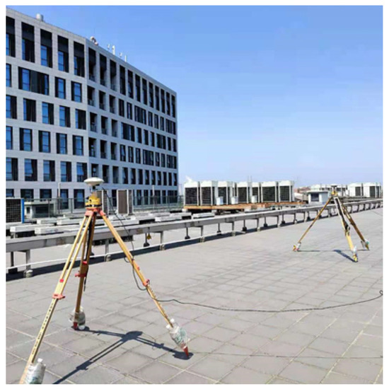
Figure 1.
Photographs of the dual antennas on the roof of a building.
The ambiguity substitution approach was implemented for the Positioning and Attitude Determination Software (PADS) procedure. PADS is designed for short-baseline data processing and attitude determination in the SD form with a common clock, and it can be operated in both real-time and post-processing modes. In this static experiment, the post-processing mode and global positioning system (GPS) L1 carrier phase observations were used. Elevation-dependent weighting was selected in the data processing, and this static experiment set the cutoff elevation to 10°. LAMBDA and bootstrapping both exist in PADS. As a widely used AR, LAMBDA was chosen to fix SD ambiguities in this study because it can find the most reliable integer ambiguity values in the ambiguity space [11,12].
3.2. The Validation of Ambiguity Substitution Approach with a Common Clock
Before evaluating the accuracy of baseline and attitude solutions based on SD observables, we need to verify whether the SD-Float ambiguities can be fixed correctly and the accuracy of the SD-Fix baseline and attitude solutions be improved by the ambiguity substitution approach.
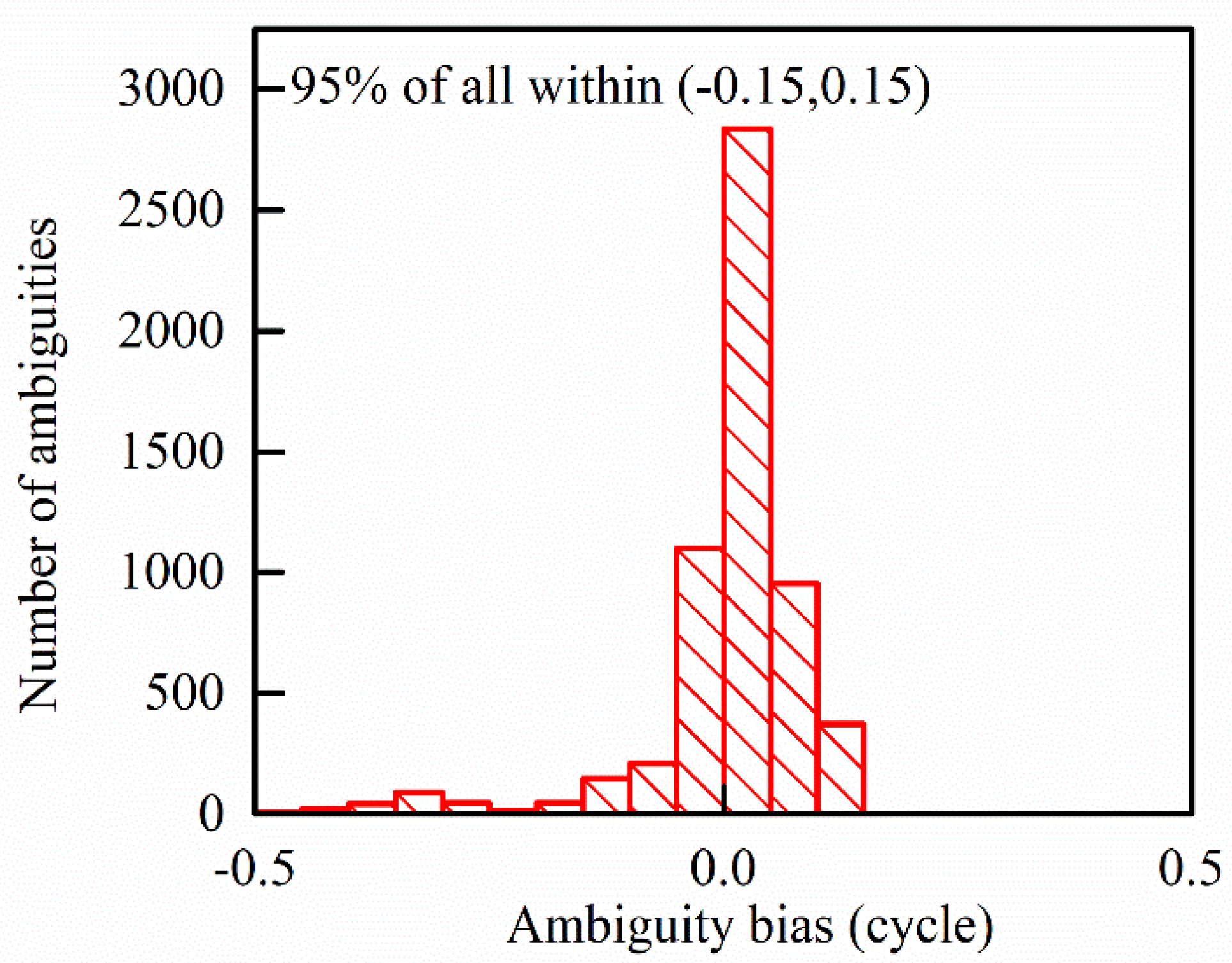
The SD-Float ambiguities should have integer characteristics after recombining with the ambiguity substitution approach. Ambiguity biases are the differences between float and fixed ambiguities; they can be used as an indicator to check whether the float ambiguity is close to an integer. Due to the real value SD UPD, this difference is assimilated by all SD ambiguity parameters if the SD UPD is not estimated. This causes systematic deviations from integers of the estimated SD ambiguities. When we introduce the SD UPD parameter and merge it with a reference ambiguity, all the remaining SD ambiguities are distributed close to integers after the real value of their common systematic deviations from integers is assimilated by the SD UPD parameter, as shown in Figure 2.
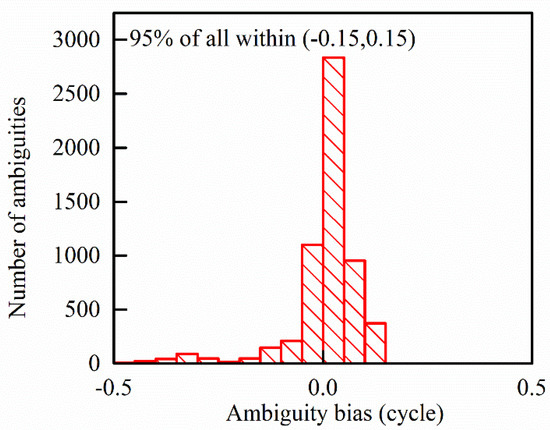
Figure 2.
The distribution of the ambiguity substitution approach SD-Float ambiguity biases.
As shown in Figure 2, more than 95% of SD-Float for the ambiguity substitution approach ambiguities are closer to an integer within 0.15 cycles. This ambiguity bias indicates that the ambiguity substitution approach can separate the SD UPD and retain the integer characteristics of SD-Float ambiguities.
After verifying the integer characteristics of the SD-Float ambiguities, the absolute biases and baseline repeatability are used to indicate the improvement of baseline precision between SD-Float and SD-Fix solutions. We used the absolute biases to compare the SD-Float and SD-Fix solutions with the reference baseline value to indicate the baseline precision. The reference baseline value is the average of multi-day solutions handled by GAMIT in static mode. The comparison of the baseline precision of the SD-Float and SD-Fix solutions for 6 days is plotted in Figure 3. The left bar in red represents the east, north, and up directions of the SD-Float solutions. The right bar in green represents the east, north, and up directions of the SD-Fix solutions by the ambiguity substitution approach. Significant improvements in baseline solutions can be achieved by fixing the SD ambiguities. The standard deviations (STDs) of SD-Fix solutions improve from (2.57, 1.64, 0.84) mm to (0.58, 0.38, 0.49) mm, or approximately by 77%, 77% and 42%, in the east, north and up directions, respectively.
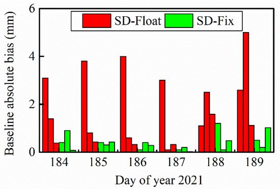
Figure 3.
Bar plots showing absolute baseline biases of SD-Float and SD-Fix solutions in east, north, and up directions for 6 days.
Although the SD-Fix baseline solutions have smaller STDs than SD-Float baseline solutions, we still need a repeatability index to reflect the degree of dispersion for the observation data. For multi-day baseline observations, after deducting the SD UPD, the baseline repeatability index should theoretically improve significantly. The daily repeatability of baselines is defined as follows [27]:
where is the number of days, and are the estimated and formal errors of the baseline component on the ith day, and is a weighted mean given by:
The daily repeatability values of SD-Float solutions, shown in Figure 4, are 1.44, 1.06, and 0.90 mm in the east, north, and up directions, respectively, while those of SD-Fix solutions are 0.73, 0.58, and 0.73 mm, respectively. Compared with SD-Float solutions, the daily repeatability improves by approximately 49%, 45%, and 19% for SD-Fix solutions in the east, north, and up directions, respectively.
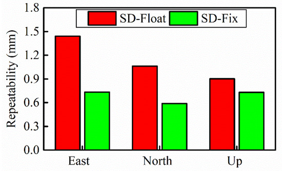
Figure 4.
Repeatability of the baseline solutions in east, north, and up directions for SD-Float and SD-Fix solutions.
3.3. Comparison of Single-Difference (SD) and Double-Difference (DD) Observables with a Common Clock in Static Mode
After comparing the SD-Fix with the SD-Float in baseline solutions and confirming the feasibility and accuracy of ambiguity substitution approach, we continue to evaluate the improvement of using BA SD observables to obtain the SD-Fix compared to DD-Fix from the perspective of practical applications. Here, the SD-Fix solutions are still obtained by PADS, based on the multi-day static observations collected in Section 3.1. We take the solutions automatically output by Trimble BD982 as the DD-Fix solutions. The baseline and attitude obtained by GAMIT in Section 3.2 are set as the truth-value to calculate the STDs and root mean squared errors (RMSEs) of the SD-Fix and DD-Fix. The data processing strategy of PADS and Trimble is given in Table 1. We try to make sure all the solutions use the same strategy in processing. Additionally, there is no information about Trimble’s methods of adjustment and AR, and we thus describe these settings as unknown.

Table 1.
Processing strategy of global positioning system (GPS) carrier phase observations for PADS and Trimble BD982.
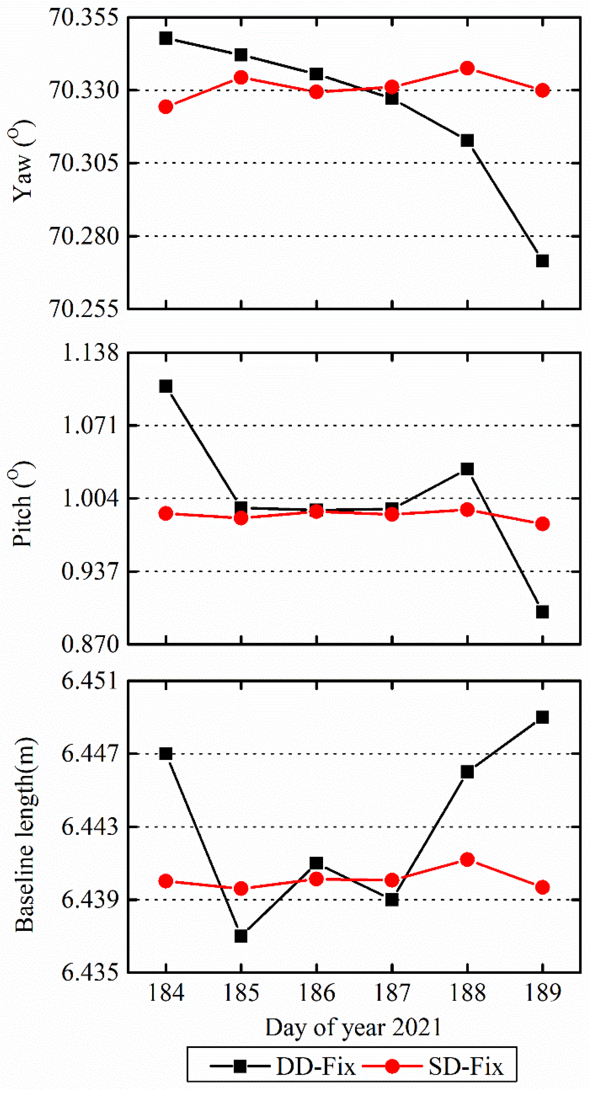
Limited by authority, our Trimble BD982 cannot output the baseline vector; we only chose the baseline attitude and length as the comparison options.
From the trend in Figure 5, the dispersions of attitude and baseline length in SD-Fix are more concentrated than DD-Fix. The STDs in Table 2 can also prove the advantage of the dispersion in SD-Fix. Compared with DD-Fix solutions, the STDs of attitude and baseline length improve by approximately 80%, 93%, and 88%, and the RMSEs of attitude and baseline length improve by approximately 80%, 93%, and 78%, respectively. These multi-day static results prove the SD observables with a common clock offer another better option for baseline and attitude solutions. It should be noted that although this trend of DD-Fix seems that Trimble has a lower attitude accuracy, nevertheless, combining with the STDs and RMSEs of DD-Fix in Table 2, both of them are lower than 0.1° for Trimble BD982. It is still a precise attitude solution for a practical application.
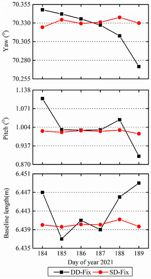
Figure 5.
Line graph of attitude and baseline length by DD-Fix and SD-Fix solutions.
Table 2.
Standard deviations (STDs) and root mean squared errors (RMSEs) of yaw, pitch angles, and baseline between DD-Fix and SD-Fix.
3.4. Comparison of Single-Difference (SD) Observables and Double-Difference (DD) Observables with a Common Clock in Kinematic Mode
The multi-day static solutions in Section 3.2 show that the SD observables with a common clock have improved baseline and attitude solutions compared with that of the DD observables. According to Chen’s theoretical derivation, under ideal conditions without multipath, the dispersion in the horizontal direction for the SD observables is equal to that of the DD observables with a common clock. The dispersion of the vertical direction for the SD observables is twice less than that of the DD observables with a common clock [6].
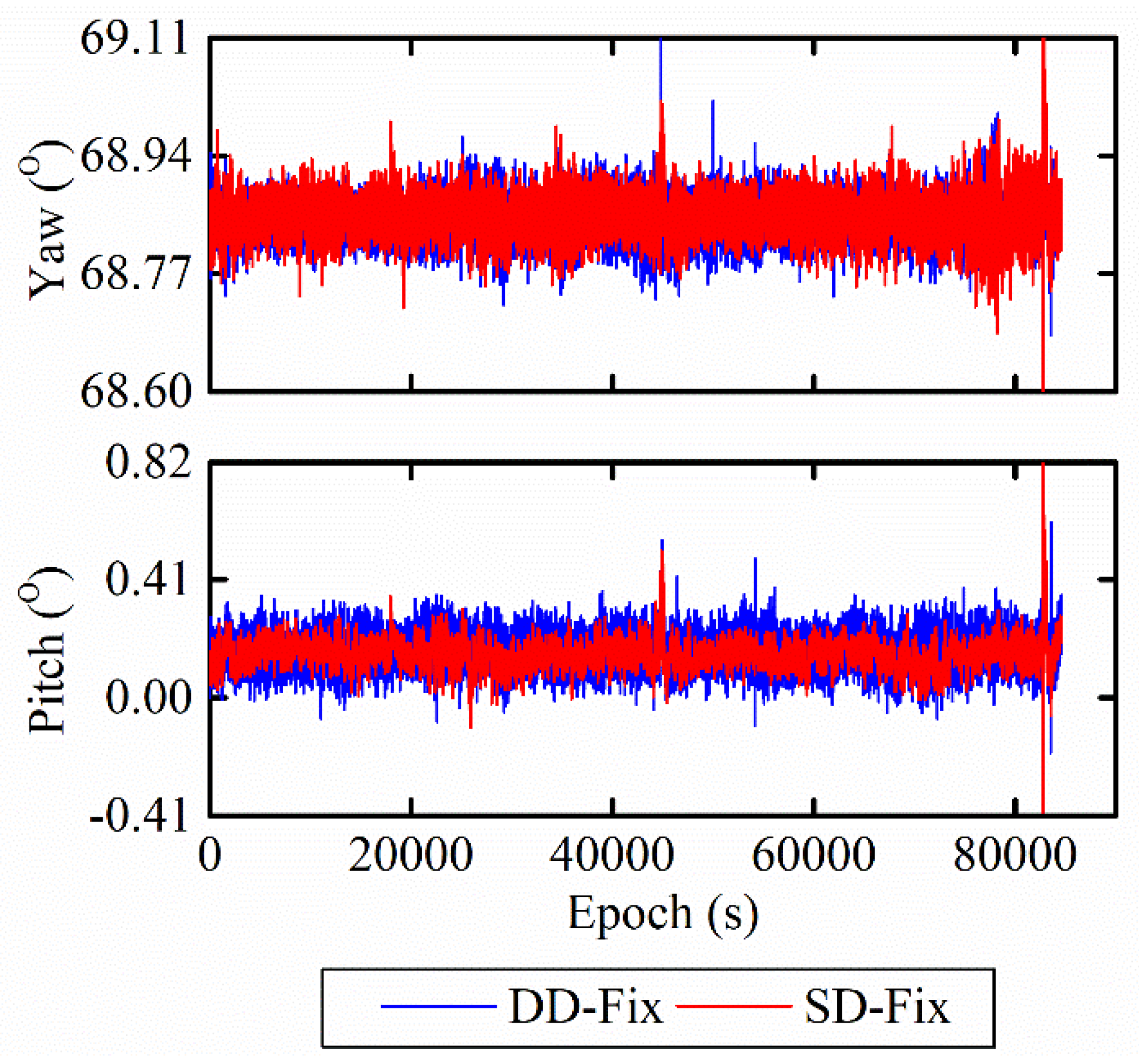
To prove the dispersion advantage of SD-Fix in one day, we selected the 5th day of the year 2021 to obtain the single-epoch kinematic attitude solution. In addition to the inconsistent baseline length, the environment and process of original observation collection are the same as the static experiment. However, for the data processing, we changed the static mode into the kinematic mode for Trimble BD982 to output the attitude solutions. In PADS, we chose the kinematic without dynamic antenna mode for state update and obtained the single-frequency and single-epoch SD-Fix attitude solutions. Other processing strategies were the same as those in Table 1. Figure 6 and Table 3 show the single-frequency and single-epoch kinematic attitude solutions without multipath mitigation.
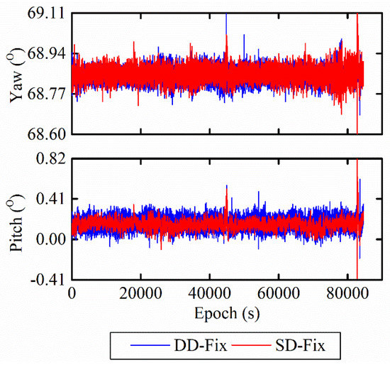
Figure 6.
Waveform showing single-frequency and single-epoch kinematic attitude solutions between DD-Fix and SD-Fix before multipath mitigation.
Table 3.
STDs of yaw and pitch angles between DD-Fix and SD-Fix before multipath mitigation /°.
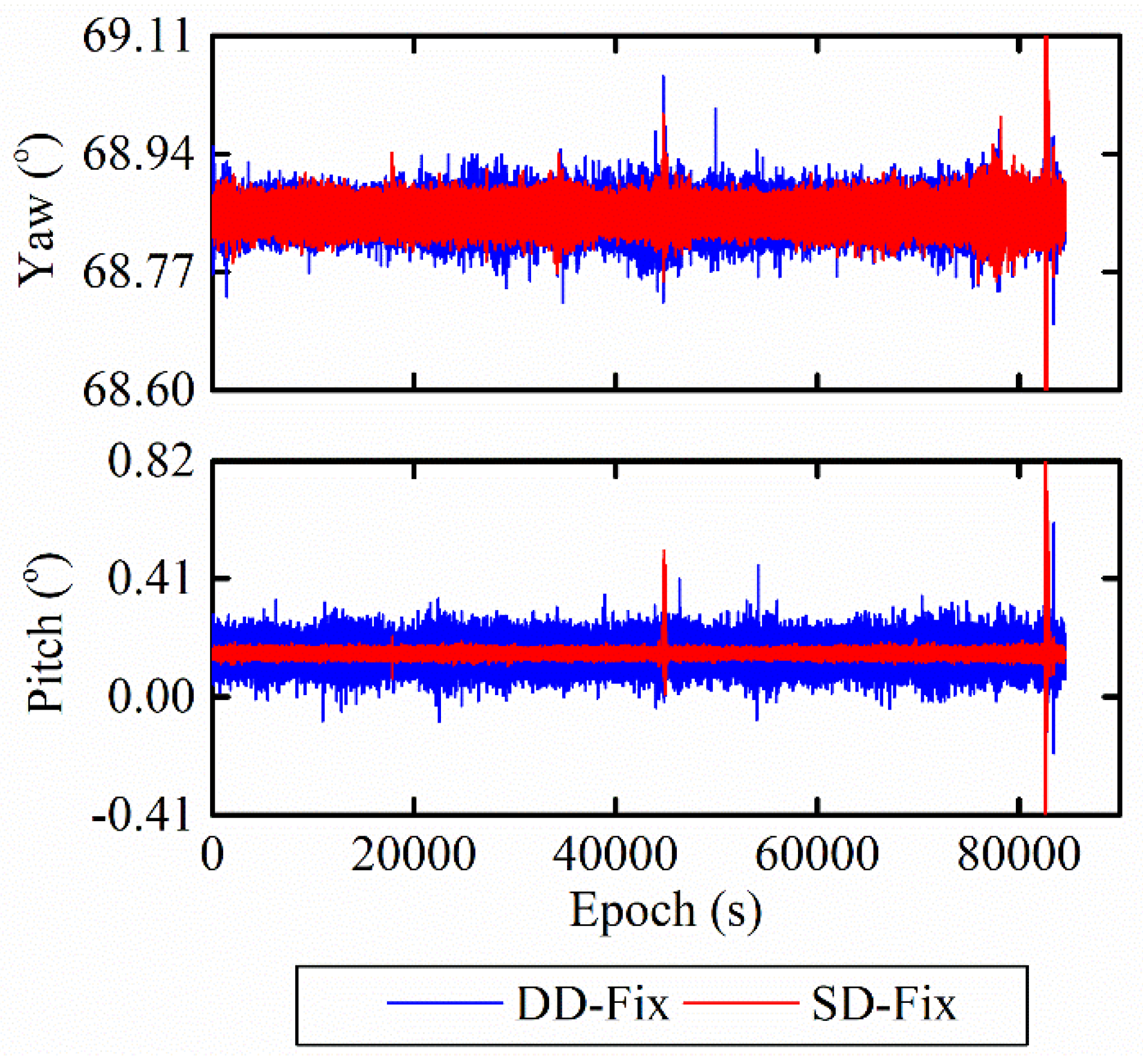
The dispersion of yaw angle for SD-Fix in Figure 6 seems the same as DD-Fix; this is consistent with most studies. However, due to the existence of multipath, the STDs of pitch angles in Table 3 are not two-fold less than that of DD-Fix. As shown in Figure 7, after extracting and eliminating the multipath in attitude solution by empirical mode decomposition (EMD) [28], the dispersion of SD-Fix is as expected smaller than that of DD-Fix. Combining with the STDs in Table 4, the STDs of pitch angles for SD-Fix can reach 0.2°, which is twice less than DD-Fix, and consistent with previous research [6].
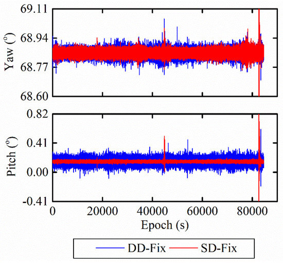
Figure 7.
Waveform showing single-frequency and single-epoch attitude solutions between DD-Fix and SD-Fix after multipath mitigation.
Table 4.
STDs of yaw and pitch angles between DD-Fix and SD-Fix after multipath mitigation /°.
Moreover, the attitude angles in Figure 6 and Figure 7 prove one limitation is that the DD observables introduce more multipath and noise than SD observables. This limitation is one of the reasons for the large dispersion of DD-Fix. On the contrary, the residuals with lower noise obtained by the SD observables are more convenient for analyzing the spatial correlation between individual satellites and satellite-elevation-dependent effects, such as in the case of GNSS stochastic models [9] and GNSS absolute antenna calibration [29].
4. The Assessment of SD Observables with a Common Clock in a Vehicle Experiment
Since the multi-antenna GNSS receiver is mostly used in dynamic scenarios, it is necessary to evaluate the performance of the SD observables in real dynamic scenarios. The vehicle experiment was carried out on the East China Normal University campus, comprising five bridges with a low pitch angle of approximately 2° to 4°, on 23 March 2015. We used a Trimble BD982 MS receiver with two Zephyr-Model 2 antennas for dynamic data collection, and the true length of the baseline was 1.75 m. As shown in Figure 8, the two antennas were parallel to the main axis of the vehicle, ensuring that the obtained attitude angles are consistent with the driving of the vehicle.
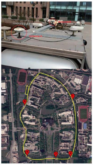
Figure 8.
Photographs of the placement of two antennas (top) and dynamic experimental trajectory (bottom).
In the process of observation collection, no threshold value for the cutoff angle was set, and the sampling frequency was 10 Hz. Additionally, we used a fiber optic gyroscope (FOG) INS KY-INS300 as a high-precision reference produced by the BDStar Navigation Company. The FOG-INS outputs a sampling frequency of 100 Hz. The car drove along the school road twice during the experiment, which was convenient for repeated verification. As for the post-processing mode, the GPS L1 carrier phase and pseudorange observations were used by PADS for the vehicle data processing, the KF with constant velocity model was used for parameters estimation, and LAMBDA was still selected as the IAR. In order to ensure the consistency of the dynamic model and other empirical disturbances, we obtained DD-Fix by estimating stochastic SD UPD every epoch. Theoretical research shows that this type of solution can be regarded as a DD solution when estimating stochastic SD UPD in every epoch.
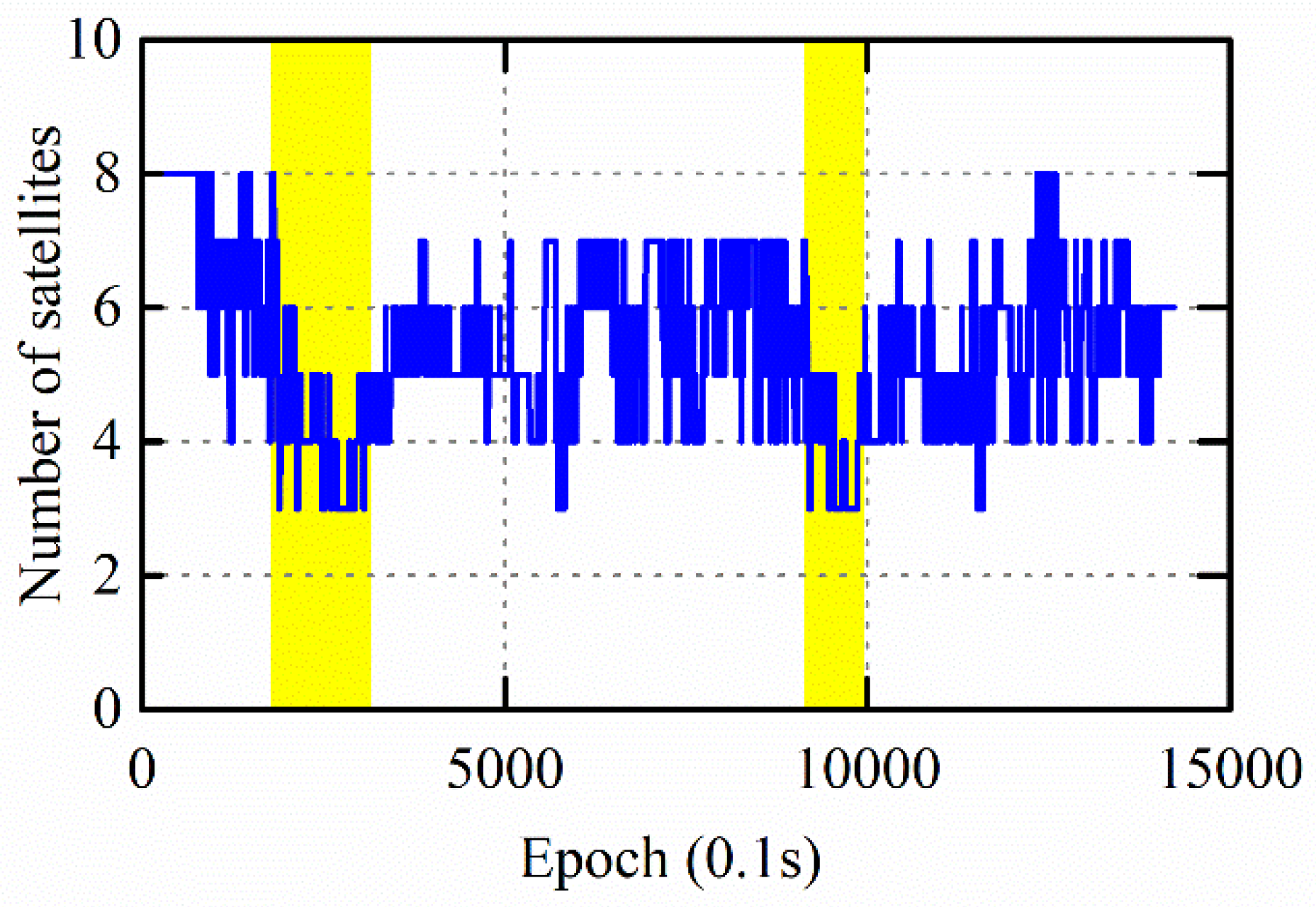
Owing to the severe blocking from nearby buildings, satellite visibility was relatively poor. On most routes, the visible satellite number was approximately 8 or less. The phase observables of all satellites were missing for a few short intervals, and only range observables were available within these intervals (Figure 9). Such an environment provides an ideal extreme experiment to examine the limitations of the SD algorithm with a common clock.

Figure 9.
Number of visible GPS satellites.
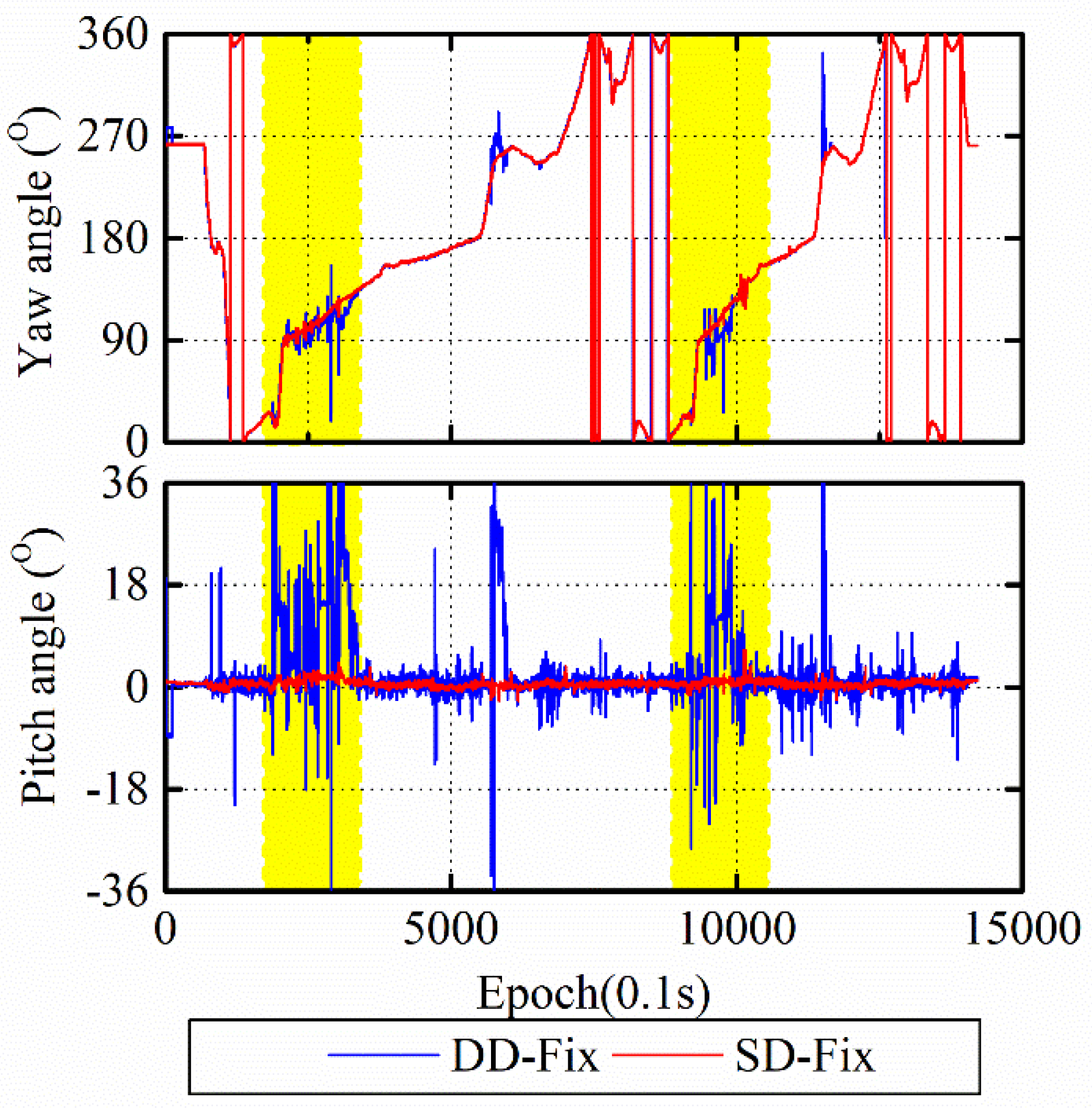
As seen from Figure 10 (top), when the number of satellites is sufficient, the performance of the yaw angle is identical between SD-Fix and DD-Fix. The number of satellites is only three, and the yaw angle diverges from the DD-Fix while the SD-Fix is still stable. This divergence is more evident in the pitch angle result in Figure 10 (bottom), and the DD-Fix cannot obtain reliable results for the pitch angle.
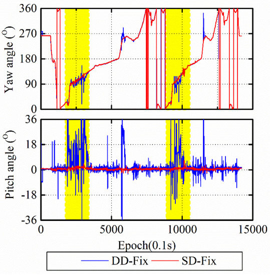
Figure 10.
Comparison of yaw (top) and pitch (bottom) angle between DD-Fix and SD-Fix.
The attitude angles in Figure 10 prove another limitation for DD observables. DD observables require at least four satellites, while SD observables only require three. This advantage allows SD observables with a common clock to have higher redundancy and more applications. Furthermore, the changeable nature of the reference satellite makes the DD data processing complicated [30]. It is easy to constitute SD observations from GNSS raw data without requiring the specification of the reference satellite, and no mathematical correlation is introduced into the observation equations [26].
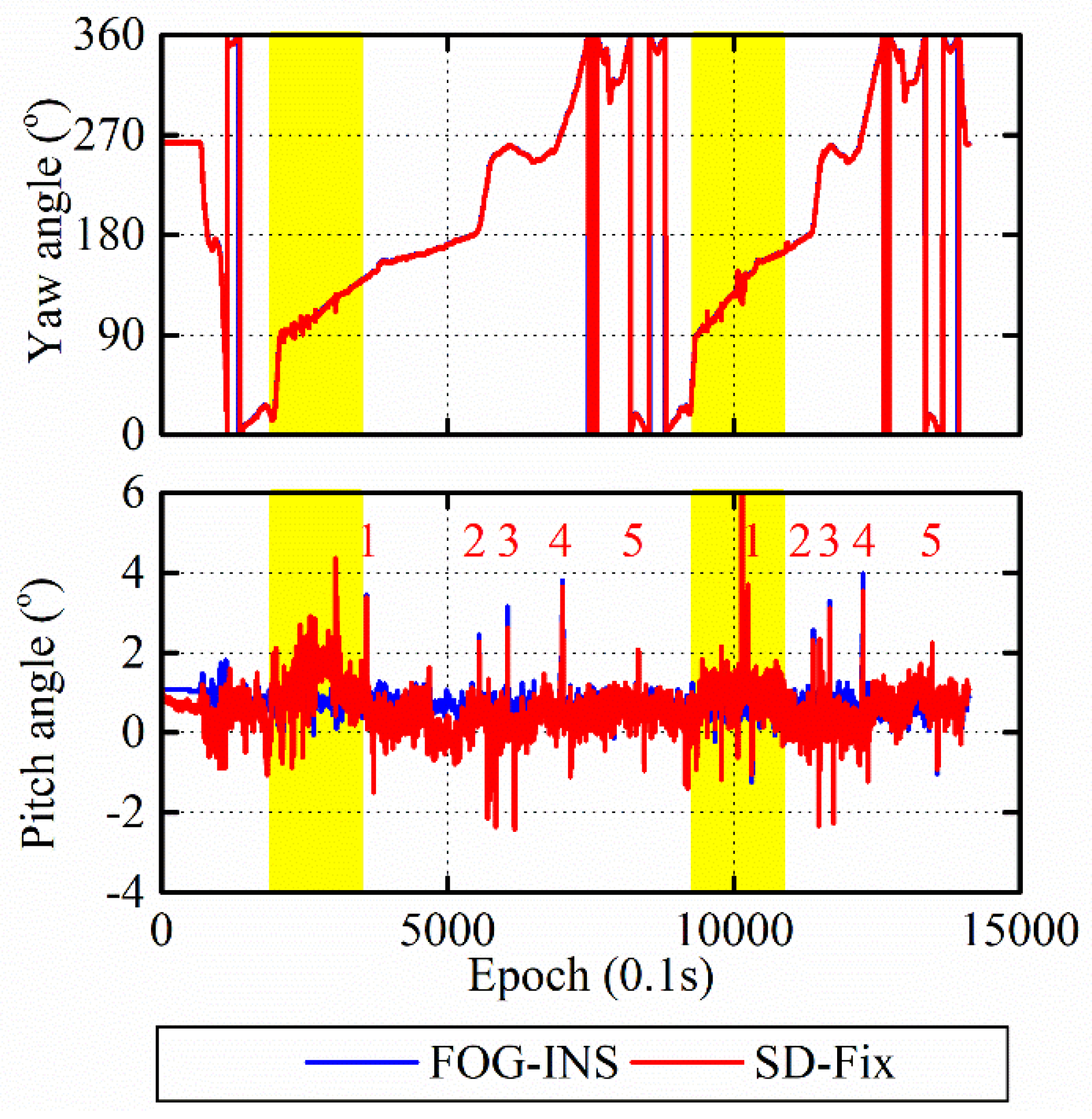
To test whether the SD observables with a common clock can detect five bridges passing along the entire route, we use the FOG-INS as a high-precision reference and ground truth. The comparison results show that the SD-Fix can still provide a stable output of the attitude solution with only three satellites. Simultaneously, it can detect five bridges with low pitch angles in the experimental route like the FOG-SINS, as shown in Figure 11, which is a task that the DD algorithm cannot perform.
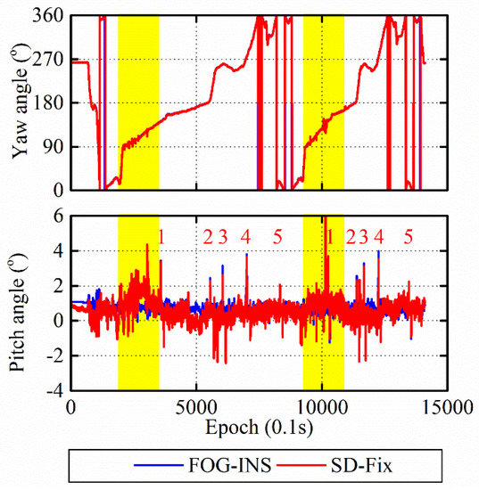
Figure 11.
Comparison of attitude between fiber optic gyroscope inertial navigation system (FOG-INS) and SD-Fix.
Table 5 evaluates the attitude angle obtained by the SD-Fix with the common clock based on the RMSEs. Considering that some of the results of DD-Fix have diverged, the RMSEs of DD-Fix are no longer given here. The RMSEs of SD-Fix in Table 5 may not seem to be particularly accurate; however, compared with the diverging DD-Fix, significant progress has been made in SD-Fix.
Table 5.
RMSEs of attitude angles for SD-Fix with common clock /°.
Additionally, although the vehicle is moving, the antenna fixed on the roof of the vehicle is stationary, so the performance of SD-Fix can also be measured by the change in the baseline length. As shown in Figure 12, the true value of the baseline length was 1.75 m. The RMSE of the baseline length sequence obtained by the SD-Fix was approximately 0.0015 m. This result also proves the reliability and stability of the SD observables. Furthermore, actual road conditions are complicated, and the environment is prominently blocked. The SD observables can still maintain good stability, demonstrating good robustness and less satellite dependence.
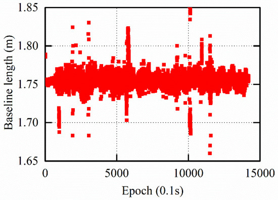
Figure 12.
Dynamic baseline length.
According to Table 5 and the residual histogram in Figure 13, there is still room for improvement in the attitude measurement performance of SD-Fix. There are several reasons for this phenomenon. First, satellite signals are blocked by many buildings in the experimental route, i.e., there are only three visible satellites in some areas. Severe multipath reduces the accuracy and stability of SD-Fix solutions, although there is no better way to eliminate this phenomenon in dynamic environments. Second, FOG-INS provides its GNSS for obtaining the initial value and then the attitude solutions by integrating, which deviates from the initial value calculated by the GNSS receiver. This result also explains why the distribution of the residual histogram in Figure 13 is symmetrical.
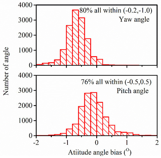
Figure 13.
Attitude angle bias between SD-Fix and FOG-INS.
5. Discussion
There are some reasons for the higher accuracy of SD observables with a common clock. On the one hand, SD observables with a common clock have stronger model strength, lower noise and ambiguity resolution success rate [6]. On the other hand, the satellite signals can be received within 360° in the horizontal direction during the observation. However, in the vertical direction satellites signals can only be received from the upper hemisphere [7]. However, problems and shortcomings still exist in SD observables with a common clock. Due to the imprecise treatment for the reference satellite, the improvement of the repeatability for the vertical direction is lower than that of horizontal direction in Figure 4. More rigorous treatments need to be output for the reference satellite. Moreover, affected by the multipath, GNSS short-baseline attitude determination still behind INS in accuracy and stability which can be seen in Figure 11 and Table 5. To further eliminate multipath and improve the accuracy and stability of the SD observables with a common clock in dynamic and complex environments will be the main work in the next stage.
6. Conclusions
The multi-antenna GNSS receiver with a common clock provides another option for high-accuracy attitude determination. Theoretical studies show that for this type of receiver, the SD and DD observable are no longer equivalent [6]. Using SD observables, the dispersion of pitch solutions is five times smaller than that using DD observables [7]. Thus, the attitude determination of the GNSS short-baseline approach can reach closer accuracy to INS in short time and greatly extend its applications if using this type of receiver and SD observables. To realize such a goal, however, the critical issue of non-zero SD UPD-caused non-integer SD ambiguities must be resolved. Since the SD UPD and ambiguities are highly correlated, direct estimating SD UPD and ambiguities becomes impossible due to rank deficiency. Past studies focused on the two-step approach, i.e., obtaining approximate SD UPD first through averaging the fractional parts for all related SD ambiguities. Then SD ambiguities are estimated by subtracting the derived SD UPD from first stage and perform integer ambiguity fixing. Our ambiguity substitution approach takes advantage of the high correlation between SD UPD and ambiguities. Owing to the high correlation, merging SD UPD with the reference satellite SD ambiguity renders all other SD ambiguities implicitly DD ambiguities, which by nature are integers and can directly utilize the DD integer resolution algorithm. Besides maintaining SD observables and removing rank deficiency, the ambiguity substitution approach also has several advantages. First, it is a one-stage approach, which is more efficient and easier to implement in real-time attitude determination. Second, it estimates redefined SD UPD with ambiguities simultaneously. There is no approximation. Third, the estimated UPD parameter can absorb time-varying perturbation due to temperature variations or rain [10]. Therefore, the solutions are more accurate and stable.
Static experiments demonstrate the effectiveness of the ambiguity substitution approach with a common clock in terms of ambiguity bias and RMSEs of multi-day baseline and attitude solutions. The RMSEs of the yaw and pitch angles obtained by the SD observables with a common clock can be improved by approximately 80% and 93%, respectively, compared to the DD observables with a common clock in multi-day attitude solutions. Additionally, the dispersion results of the kinematic attitude solution proved that the accuracy of SD observables with a common clock is higher than the DD observables with a common clock in the vertical direction of the attitude solution. The results of the static and kinematic experiments support the vehicle experiment. In the vehicle experiment, the SD observables with a common clock successfully detected five bridges with small pitch angles like the FOG-INS, which the DD observables were unable to do. This high sensitivity in pitch angle can be combined with INS and used in attitude determination of ships, missiles, autopilots, etc. Thus, attention should be given to a multi-antenna GNSS receiver that uses the SD observables with a common clock.
Author Contributions
Conceptualization, D.D. and W.C.; methodology, D.D. and C.Z.; software, C.Z.; validation, D.D., M.C. and C.Z.; formal analysis, W.C.; investigation, M.C. and C.Z.; resources, W.C. and J.W.; data curation, Y.P. and C.Y.; writing—original draft preparation, C.Z.; writing—review and editing, D.D.; visualization, C.Z.; supervision, W.C.; project administration, W.C.; funding acquisition, W.C. All authors have read and agreed to the published version of the manuscript.
Funding
This research was funded by National Natural Science Foundation of China, grant number No. 41771475; Social Development Project of Science and Technology Innovation Action Plan of Shanghai, grant number No. 20dz1207107; the Fund of Director of Key Laboratory of Geographic Information Science (Ministry of Education), East China Normal University, grant number No. KLGIS2020C05” and The APC was funded by National Natural Science Foundation of China, grant number No. 41771475.
Acknowledgments
We would like to thank Feng Zhou, Xingwang Zhao and Xinyun Cao for their suggestions in the research process.
Conflicts of Interest
The authors declare no conflict of interest.
References
- Zhang, P.; Zhao, Y.; Lin, H.; Zou, J.; Wang, X.; Yang, F. A Novel GNSS Attitude Determination Method Based on Primary Baseline Switching for A Multi-Antenna Platform. Remote Sens. 2020, 12, 747. [Google Scholar] [CrossRef] [Green Version]
- Wu, S.; Zhao, X.; Pang, C.; Zhang, L.; Xu, Z.; Zou, K. Improving ambiguity resolution success rate in the joint solution of GNSS-based attitude determination and relative positioning with multivariate constraints. GPS Solut. 2020, 24, 31. [Google Scholar] [CrossRef]
- Zhang, S.; Chang, G.; Chen, C.; Chen, G.; Zhang, L. Parameterization-switching GNSS attitude determination considering the success rate of ambiguity resolution. Meas. Sci. Technol. 2020, 31, 065105. [Google Scholar] [CrossRef]
- Medina, D.; Vilà-Valls, J.; Hesselbarth, A.; Ziebold, R.; García, J. On the Recursive Joint Position and Attitude Determination in Multi-Antenna GNSS Platforms. Remote Sens. 2020, 12, 1955. [Google Scholar] [CrossRef]
- Dong, D.; Chen, W.; Cai, M.; Zhou, F.; Wang, M.; Yu, C.; Zheng, Z.; Wang, Y. Multi-antenna synchronized global navigation satellite system receiver and its advantages in high-precision positioning applications. Front. Earth Sci. 2016, 10, 772–783. [Google Scholar] [CrossRef]
- Chen, W.; Qin, H.; Zhang, Y.; Jin, T. Accuracy assessment of single and double difference models for the single epoch GPS compass. Adv. Space Res. 2012, 49, 725–738. [Google Scholar] [CrossRef]
- Chen, W.; Yu, C.; Dong, D.; Cai, M.; Zhou, F.; Wang, Z.; Zhang, L.; Zheng, Z. Formal Uncertainty and Dispersion of Single and Double Difference Models for GNSS-Based Attitude Determination. Sensors 2017, 17, 408. [Google Scholar] [CrossRef] [Green Version]
- Wang, Z.; Chen, W.; Dong, D.; Wang, M.; Cai, M.; Yu, C.; Zheng, Z.; Liu, M. Multipath mitigation based on trend surface analysis applied to dual-antenna receiver with common clock. GPS Solut. 2019, 23, 104. [Google Scholar] [CrossRef]
- Liu, X. A comparison of stochastic models for GPS single differential kinematic positioning. In Proceedings of the 15th International Technical Meeting of the Satellite Division of the Institute of Navigation (ION GPS 2002), Portland, OR, USA, 24–27 September 2002; pp. 1830–1841. [Google Scholar]
- Liang, Z.; Yanqing, H.; Jie, W. A drift line bias estimator: ARMA-based filter or calibration method, and its application in BDS/GPS-based attitude determination. J. Geod. 2016, 90, 1331–1343. [Google Scholar] [CrossRef]
- Teunissen, P.J.G. Least-squares estimation of the integer GPS ambiguities. Presented at the General Meeting of the International Association of Geodesy, Beijing, China, 8–13 August 1993. [Google Scholar]
- Teunissen, P.J.G. The least-squares ambiguity decorrelation adjustment: A method for fast GPS integer ambiguity estimation. J. Geod. 1995, 70, 65–82. [Google Scholar] [CrossRef]
- Giorgi, G. The Multivariate Constrained LAMBDA Method for Single-epoch, Single-frequency GNSS-based Full Attitude Determination. In Proceedings of the 23rd International Technical Meeting of the Satellite Division of The Institute of Navigation (ION GNSS 2010), Portland, OR, USA, 21–24 September 2010; pp. 1429–1439. [Google Scholar]
- Ma, L.; Lu, L.; Zhu, F.; Liu, W.; Lou, Y. Baseline length constraint approaches for enhancing GNSS ambiguity resolution: Comparative study. GPS Solut. 2021, 25, 40. [Google Scholar] [CrossRef]
- Teunissen, P.J.G.; Giorgi, G.; Buist, P.J. Testing of a new single-frequency GNSS carrier phase attitude determination method: Land, ship and aircraft experiments. GPS Solut. 2011, 15, 15–28. [Google Scholar] [CrossRef] [Green Version]
- Dong, D.; Bock, Y. Global Positioning System Network analysis with phase ambiguity resolution applied to crustal deformation studies in California. J. Geophys. Res. Solid Earth 1989, 94, 3949. [Google Scholar] [CrossRef]
- Teunissen, P.J.G. Success probability of integer GPS ambiguity rounding and bootstrapping. J. Geod. 1998, 72, 606–612. [Google Scholar] [CrossRef] [Green Version]
- Chen, W.; Li, X. Success rate improvement of single epoch integer least-squares estimator for the GNSS attitude/short baseline applications with common clock scheme. Acta Geod. Geophys. 2014, 49, 295–312. [Google Scholar] [CrossRef]
- Li, Y.; Zhang, K.; Roberts, C.; Murata, M. On-the-fly GPS-based attitude determination using single- and double-differenced carrier phase measurements. GPS Solut. 2004, 8, 93–102. [Google Scholar] [CrossRef]
- Laurichesse, D.; Mercier, F.; Berthias, J.-P.; Broca, P.; Cerri, L. Integer Ambiguity Resolution on Undifferenced GPS Phase Measurements and Its Application to PPP and Satellite Precise Orbit Determination. Navigation 2009, 56, 135–149. [Google Scholar] [CrossRef]
- Collins, P.; Bisnath, S.; Lahaye, F.; Héroux, P. Undifferenced GPS Ambiguity Resolution Using the Decoupled Clock Model and Ambiguity Datum Fixing. Navigation 2010, 57, 123–135. [Google Scholar] [CrossRef] [Green Version]
- Leick, A.; Rapoport, L.; Tatarnikov, D. GPS Satellite Surveying, 4th ed.; John Wiley & Sons, Inc.: Hoboken, NJ, USA, 2015; pp. 129–207. [Google Scholar]
- Xu, G.; Xu, Y. GPS: Theory, Algorithm and Applications, 3rd ed.; Springer-Verlag: Berlin/Heidelberg, Germany, 2007; pp. 63–133. [Google Scholar]
- Ge, M.; Gendt, G.; Rothacher, M.; Shi, C.; Liu, J. Resolution of GPS carrier-phase ambiguities in Precise Point Positioning (PPP) with daily observations. J. Geod. 2008, 82, 389–399. [Google Scholar] [CrossRef]
- Geng, J.; Teferle, F.N.; Shi, C.; Meng, X.; Dodson, A.H.; Liu, J. Ambiguity resolution in precise point positioning with hourly data. GPS Solut. 2009, 13, 263–270. [Google Scholar] [CrossRef] [Green Version]
- Chen, W. A remark on the GNSS single difference model with common clock scheme for attitude determination. J. Appl. Geod. 2016, 10, 167–173. [Google Scholar] [CrossRef]
- Blewitt, G. Carrier phase ambiguity resolution for the Global Positioning System applied to geodetic baselines up to 2000 km. J. Geophys. Res. Solid Earth 1989, 94, 10187–10203. [Google Scholar] [CrossRef] [Green Version]
- Li, Q.; Xia, L.; Chan, T.O.; Xia, J.; Geng, J.; Zhu, H.; Cai, Y. Intrinsic Identification and Mitigation of Multipath for Enhanced GNSS Positioning. Sensors 2020, 21, 188. [Google Scholar] [CrossRef] [PubMed]
- Bilich, A.; Mader, G.L. GNSS absolute antenna calibration at the national geodetic survey. In Proceedings of the 23rd International Technical Meeting of the Satellite Division of The Institute of Navigation (ION GNSS 2010), Portland, OR, USA, 21–24 September 2010; pp. 1369–1377. [Google Scholar]
- Chang, X.; Paige, C.C. Two carrier phase based approaches for autonomous fault detection and exclusion. In Proceedings of the 13th International Technical Meeting of the Satellite Division of The Institute of Navigation (ION GPS 2000), Salt Lake City, UT, USA, 19–22 September 2000; pp. 1895–1905. [Google Scholar]


Publisher’s Note: MDPI stays neutral with regard to jurisdictional claims in published maps and institutional affiliations. |
© 2021 by the authors. Licensee MDPI, Basel, Switzerland. This article is an open access article distributed under the terms and conditions of the Creative Commons Attribution (CC BY) license (https://creativecommons.org/licenses/by/4.0/).