Article

Development and Testing of a UAV-Based Multi-Sensor System for Plant Phenotyping and Precision Agriculture

1
Bio-Sensing and Instrumentation Laboratory, College of Engineering, The University of Georgia, Athens, GA WJXF 63, USA
2
Phenomics and Plant Robotics Center, The University of Georgia, Athens, GA WJXF 63, USA
3
Center for Geospatial Research, The University of Georgia, Athens, GA WJXF 63, USA
*
Author to whom correspondence should be addressed.
Remote Sens. 2021, 13(17), 3517; https://doi.org/10.3390/rs13173517
Submission received: 18 June 2021 / Revised: 27 August 2021 / Accepted: 29 August 2021 / Published: 4 September 2021
(This article belongs to the Special Issue Remote Sensing for Precision Agriculture)

Abstract

:
Unmanned aerial vehicles have been used widely in plant phenotyping and precision agriculture. Several critical challenges remain, however, such as the lack of cross-platform data acquisition software system, sensor calibration protocols, and data processing methods. This paper developed an unmanned aerial system that integrates three cameras (RGB, multispectral, and thermal) and a LiDAR sensor. Data acquisition software supporting data recording and visualization was implemented to run on the Robot Operating System. The design of the multi-sensor unmanned aerial system was open sourced. A data processing pipeline was proposed to preprocess the raw data and to extract phenotypic traits at the plot level, including morphological traits (canopy height, canopy cover, and canopy volume), canopy vegetation index, and canopy temperature. Protocols for both field and laboratory calibrations were developed for the RGB, multispectral, and thermal cameras. The system was validated using ground data collected in a cotton field. Temperatures derived from thermal images had a mean absolute error of 1.02 °C, and canopy NDVI had a mean relative error of 6.6% compared to ground measurements. The observed error for maximum canopy height was 0.1 m. The results show that the system can be useful for plant breeding and precision crop management.

1. Introduction

High-throughput phenotyping is a method of using sensing and automation technologies to measure phenotypic traits in order to accelerate breeding programs for major crops [1] in support of increased plant productivity and resilience to biotic and abiotic stresses impacting plant health and growth. Traditional methods for collecting field data to support crop breeding require significant human labor. As a result, designing an automatic phenotyping platform to work in the field has attracted the attention of researchers in both plant science and engineering communities. Early solutions for an automatic data collection platform utilized ground vehicles (either tractor or robotic platforms) equipped with sensors to acquire the desired data [2,3,4]. During data collection, ground vehicles are driven either manually or automatically through each plot, and data are collected and stored in a data logger or computer. Ground vehicles have the advantage of supporting large payloads and can easily carry multiple sensors simultaneously. In addition, these vehicles can control the data collection environment, for instance, by using enclosures to guarantee data quality and to ensure similar acquisition conditions (e.g., illumination and wind). Ground platforms also have several disadvantages, however, including low data scanning speed, the need to adjust planting layout for certain crops to accommodate vehicle characteristics, soil compaction resulting from frequent data collection, and challenges of adapting the platform to different crops once the design is fixed.
Unmanned aerial vehicles (UAVs) offer an alternative to ground data collection in support of high-throughput phenotyping and can address disadvantages of ground vehicles to some degree. Compared to ground platforms, UAVs can provide higher data scanning speed and can cover relatively larger fields. Due to the physical separation from plants, UAVs can be adapted easily to different types of crops and at different growth stages. Furthermore, UAVs can be controlled automatically by their onboard autopilot system; thus, they require less human intervention during data collection. Limitations of UAVs include reduced payload when compared to ground vehicles, resulting in equipment weight restrictions. In addition, the quality of data collected by UAVs is more likely to be affected by the environment due to lack of environmental controls. The spatial resolution of aerial data is usually lower than that of ground systems.
There have been many studies on UAV-based high-throughput phenotyping published in recent years [5,6,7], and a variety of sensors have been integrated into UAV platforms, including multiple types of cameras (RGB, thermal, multispectral, and hyperspectral) and Light Detection and Ranging (LiDAR) sensors [8]. Cameras and LiDAR can provide spatial and spectral information about plants, which can be used to measure directly or indirectly various phenotypic traits. RGB images can be used to estimate leaf area index (LAI), crop emergence, and to count flowers [9,10,11]. The Structure from Motion (SfM) technique can be used with RGB images to generate a Digital Surface Model (DSM), which can be used to estimate plant height, predict biomass/yield, detect crop lodging, and derive canopy structure metrics [12,13,14,15,16]. Multispectral imaging can provide vegetation indices, such as the widely used Normalized Difference Vegetation Index (NDVI), which have proven to correlate with leaf area index, plant disease, plant nutrient deficiency, and yield [17,18,19,20,21]. Thermal images have been used frequently to measure canopy temperature, which is an indicator of stomatal conductance and plants’ response to water stress [22,23]. Therefore, thermal images can be used to detect water stress [24,25,26]. Hyperspectral imaging provides more detailed spectral information of targets when compared to multispectral cameras and can be used to further monitor plants’ physiological status and related processes [27]. For example, one study showed that the Photochemical Reflectance Index (PRI) from hyperspectral imaging can be used to access the water stress in maize [28], whereas several other studies applied hyperspectral images to estimate biomass and yield, as well as to detect plant diseases [29,30,31,32].
Despite the great potential and progress in the field of UAVs when applied to high-throughput phenotyping, several application challenges remain to be further studied. First, most UAV platforms have been designed based on a particular aerial vehicle and one or more sensors. For example, although multi-sensor UAV systems were developed to acquire complementary information to measure complex phenotypic traits such as water stress and yield [33,34], these systems are typically limited to up to two specific sensors without flexible data acquisition software system that can adapt to new sensors. Rigid designs are difficult to expand, adapt to other needs, and reuse for other research or applications. This limitation can be circumvented by designing a multi-sensor data acquisition system that can be deployed on different UAV platforms. Second, since sensors are affected by environmental conditions that could make the data collected from different sessions inconsistent and non-comparable, calibration methods need to be developed for different types of sensors. For example, thermal images are affected by the atmosphere and need to be calibrated properly using environmental data to obtain accurate thermal readings [35]. Lastly, converting sensor data into meaningful phenotypic traits for variety selection and plant growth assessment requires a complex set of data processing algorithms and tools. Therefore, designing a framework that can incorporate existing and future algorithms remains a major task for researchers. Additionally, although UAVs have been used widely for plant phenotyping, it has remained a challenge for researchers without an engineering background to develop a feature-rich data collection UAV system.
In order to address the above challenges, the main goal of this paper is to design a flexible unmanned aerial data acquisition system as well as an airborne sensor calibration and data processing framework that can be used by researchers in phenomics and precision agriculture. Specific objectives include the following: (1) Designing a data acquisition system that can be attached easily to different UAV platforms, (2) developing camera calibration protocols that are transferable to other data collection efforts, and (3) designing a data processing pipeline for extracting phenotypic traits from the raw data. The design of the system was open-sourced and is available to researchers and other individuals.

2. System Design

We adopted a modularized approach to design the unmanned aerial system (UAS), aiming to separate the full system into an aerial platform and a data acquisition system (DAS). In this manner, the DAS can be carried by different aerial platforms or even by ground platforms. We designed two versions of DAS over the past five years. The first version consists of a DSLR camera (Lumix G6, Panasonic, Kadoma, Japan), a multispectral camera (RedEdge, MicaSense, Seattle, WA, USA), and a thermal camera (Tau 2, FLIR Systems, Wilsonville, OR, USA) (Table 1). This version of the DAS has a simpler design and does not include the Robot Operating System (ROS). The second version of the DAS replaced the DSLR camera with an industrial camera (GrassHopper3, FLIR Systems, Wilsonville, OR, USA) and added a 3D LiDAR sensor (VLP-16, Velodyne Lidar, CA, USA). In addition, this DAS has an improved mechanical design and can be controlled using ROS. This paper briefly introduces the design of the first version of the DAS and focuses on the development of the second version.

2.1. First Version of the Data Acquisition System

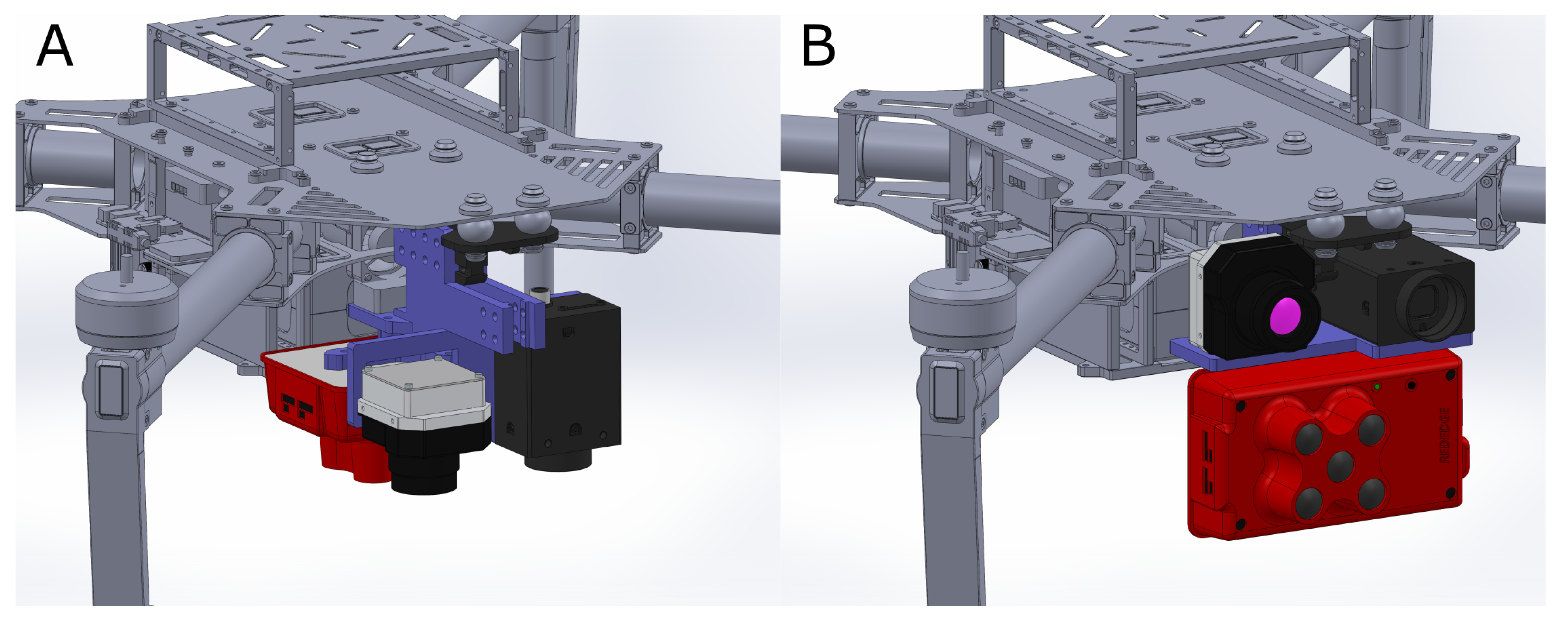
The DSLR, multispectral, and thermal cameras integrated into this DAS were controlled by a single-board computer (Raspberry Pi 3) (Figure 1A). The cameras and Raspberry Pi were mounted on a camera case, which was attached to a high payload UAV (S1000+, DJI, Shenzhen, China) (Figure 1B). A GNSS/IMU (VN200, VectorNav, Dallas, TX, USA) was used to record the position and pose of the images. Two DC-DC converters were used to power the thermal and the multispectral cameras, as well as the Raspberry Pi (power supplied by the UAV). Software was developed to run on the Raspberry Pi triggered cameras and saved thermal images and geolocation to the on-board memory.

2.2. Second Version of the Data Acquisition System

The second version of the DAS consisted of three imaging sensors (thermal, industrial RGB, and multispectral cameras), a LiDAR sensor, and a single-board computer (Manifold, DJI, China). For simplicity, the remainder of this paper will use RGB camera to refer to the industrial RGB camera. Table 1 lists specifications for the sensors. All sensors were connected mechanically by a sensor bracket, which was designed in CAD software and fabricated by using a 3D printer. All CAD designs created for this implementation were open-sourced and can be downloaded from our GitHub (https://github.com/UGA-BSAIL/UAS_sensor_mount, accessed on 18 June 2021).
Sensor brackets (blue part in Figure 2) were printed in ABS plastic using a 3D printer (uPrint SE Plus, Stratasys, Eden Prairie, MN, USA). Connection brackets (green parts in Figure 2) are used to connect the DAS to the UAV and were printed in carbon fiber by using another 3D printer (Markforged Onyx Pro, Markforged, Watertown, MA, USA) to enhance the strength of connection. Connection brackets have a slide slot which allows easy attachment and detachment of the DAS to and from the UAV. The DAS also can be carried by other rotatory UAVs with adequate payload to carry the DAS. Connection brackets may need to be redesigned to fit the specific drone.
Each camera is mounted to a bracket; thus, the camera can be individually detached from the DAS and used as an independent system. This flexibility benefits multiple use cases, including when only images are needed or only low-payload UAVs are available. Cameras can be assembled to work horizontally or vertically (Figure 3). Frontward facing cameras can benefit applications that require a side-looking view of plants, such as imaging between rows of a vineyard. The vertical mount can be used to acquire nadir views of plant canopies.

2.2.1. Electronic Design

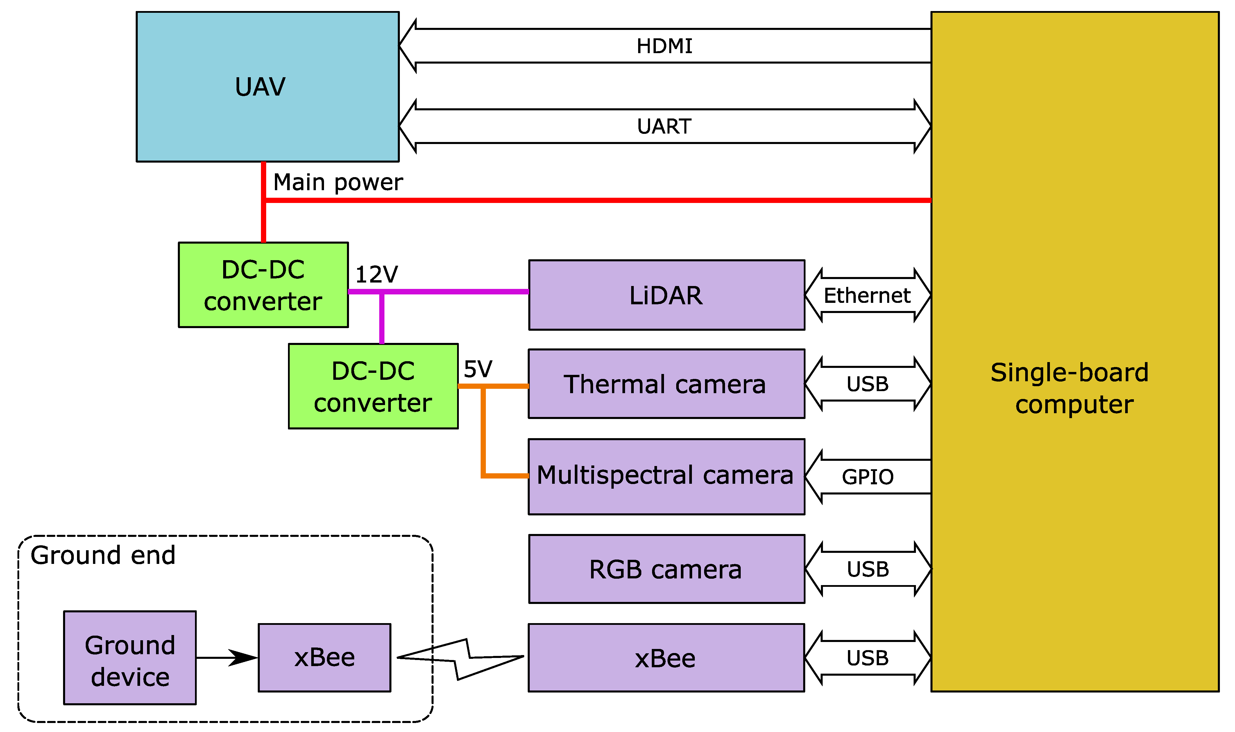
The main power (18 V ) of the DAS comes from the UAV and directly powers the single-board computer. A DC-DC converter is used to convert the main power to 12 V and another DC-DC to convert 12 V to 5 V (Figure 4). The LiDAR is powered at 12 V , the thermal and multispectral cameras are powered at 5 V , and the RGB camera is powered at 5 V through the USB port from the single-board computer. The DAS can be powered with a voltage source from 14 V to 26 V .
The single-board manifold computer, running Ubuntu 14.04 armhf, is used to control sensors and to acquire data from the sensors (Figure 4). Controlling the RGB and thermal cameras is achieved through USB and images are transmitted through USB. LiDAR data are transmitted to the single-board computer through Ethernet. Since the multispectral camera is an independent system that has its own image processing and storing capabilities, we only implemented a trigger function through a GPIO pin to synchronize collection with other cameras. Complete control of the multispectral camera is also possible by using the serial and Ethernet interfaces on the camera. The single-board computer can interface with the UAV through the Universal Asynchronous Receiver/Transmitter (UART) to obtain real-time flight data (e.g., position and posing of the vehicle). However, additional positioning hardware (GNSS and IMU) is needed for data post processing if the design incorporates a UAV platform that cannot output its flight data. The High-Definition Multimedia Interface (HDMI) port of the single-board computer is connected to the HDMI transmitter on the UAV so that the user can see the Ubuntu desktop in real-time.
The FLIR Tau 2 camera originally only provided a 50-pin interface that includes a parallel digital port to output digital data. We designed a circuit based on the Cypress EZ-USB chip (CY7C68013A, Cypress Semiconductor, San Jose, CA, USA) to convert the parallel digital output to a USB protocol so that it could interface with the single-board computer through a USB port. This circuit makes it possible to acquire raw digital radiometric data from the camera without using a frame grabber. In order to support the calibration of the thermal camera, ground data including atmospheric conditions (air temperature, humidity, and air pressure) and temperature of the thermal calibration targets were recorded by using a customized device. The ground data are transmitted to the single-board computer in real time through xBee (xBee Pro S1, Digi International, Hopkins, MA, USA).

2.2.2. Software Design

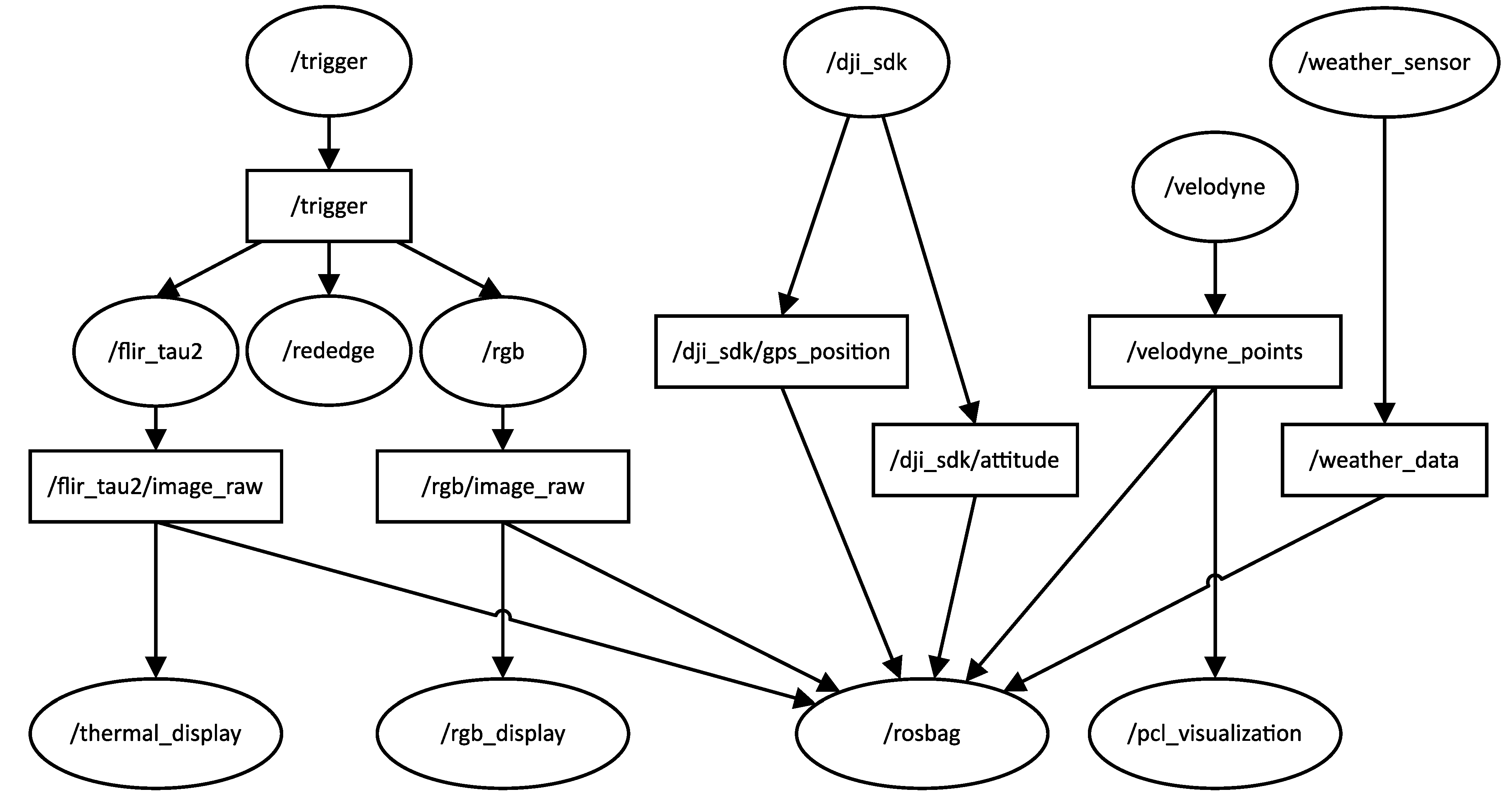
The data acquisition software was implemented by using the Robot Operating System (ROS) release indigo running on the single-board computer (Figure 5). Implemented nodes include the following: flir_tau2 (retrieves raw digital images from the thermal camera), rededge (triggers the multispectral camera), rgb (captures RGB images), and velodyne (obtains LiDAR data). All cameras are synchronized through the trigger topic. We use the ROS package dji_sdk provided by DJI to obtain UAV location and pose. The weather_sensor node is used to receive data from the sensor on the station and to publish atmospheric data as a ROS topic. Data recordings are conducted by the rosbag node. The rosbag node saves the sensor data, drone flight data, and weather data to a bag file.
Three data visualization nodes, thermal_display, rgb_display, and pcl_visualization, were implemented to visualize the RGB image, thermal image, and the LiDAR data. Data visualization nodes create a window on the Ubuntu desktop, allowing users to display and monitor sensor data in real time through radio transmission. In addition, users can check ROS topics on a ground computer, if the computer and the single-board computer flying on the UAV are connected to the same wireless network.

3. Camera Calibration

3.1. Geometric Calibration

Geometric calibration included the estimation of geometric parameters of cameras, which were used to correct for lens distortion. We used the Camera Calibrator app from MATLAB (MATLAB 2018, MathWorks, Natick, MA, USA) to find calibration parameters for each camera, including the parameters for the camera’s intrinsic matrix, radial distortion model (Equation (1)), and tangential distortion model (Equation (2)) [36]:
x d i s t o r t e d y d i s t o r t e d = ( 1 + k 1 r 2 + k 2 r 4 + k 3 r 6 ) x y
x d i s t o r t e d y d i s t o r t e d = x y + 2 p 1 x y + p 2 ( r 2 + 2 x 2 ) p 1 ( r 2 + 2 y 2 ) + 2 P 2 x y
where r = ( x x p ) 2 + ( y y p ) 2 is the distance between the pixel ( x , y ) to the principal point ( x p , y p ) , k 1 , k 2 , k 3 are radial distortion coefficients of the lens, and p 1 , p 2 are tangential distortion coefficients of the lens.
In order to calibrate the RGB and multispectral cameras we used a chessboard pattern printed on white paper. Two tungsten halogen lamps were used for the multispectral camera to provide additional light sources for the NIR band. For the thermal camera, a chessboard pattern was printed using a poster printer. The difference in emissivity between the ink and the paper was used to create the pattern when collecting thermal images, and four heat lamps were used to heat the printed chessboard in order to enhance the definition of the pattern. The grid size of the chessboard is 21   mm × 21   mm for the RGB and multispectral cameras and 110   mm × 110   mm for the thermal camera. A larger chessboard pattern was used for the thermal camera because that camera needs to collect images at a larger distance for images to be in focus. Each camera was used to collect ten images from different angles.

3.2. Vignetting Calibration

Vignetting is an effect of the radial falloff of intensity from the center of the image, including natural vignetting, pixel vignetting, optical vignetting, and mechanical vignetting [37]. There are two methods to model the vignetting effect. The first method models vignetting ( V x , y ) as a high order polynomial (Equation (3)) and assumes zero vignetting effect ( V ( x v , y v ) = 1 ) at the center of vignetting ( x v , y v ) :
V ( x , y ) = V ( r ) = 1 + α 1 r + α 2 r 2 + α 3 r 3 + α 4 r 4 + α 5 r 5 + α 6 r 6
r = ( x x v ) 2 + ( y y v ) 2
where r is the distance of the pixel from the center of vignetting, and α 1 to α 6 are the model parameters.
The second method models the vignetting effect as a look up table that stores the correction coefficients for each pixel. The second method can provide more accurate results, but it requires multiple tables for different camera settings. Since the first method is simple to implement and has been considered effective, it was chosen to model the vignetting of the multispectral camera.
In order to calculate model parameters, we measured the vignetting effect by imaging a scene with uniform luminance. For the multispectral camera, we used an integrating sphere to create such a scene. The setup of the integrating sphere is similar to [38], but we added a Teflon sheet to cover the exit port so the light could be more evenly distributed after passing the Teflon sheet. A black body was used for the same purpose for the thermal camera. We collected ten images for each camera and used the mean image to find the model parameters. The parameters ( x v , y v and α 1 to α 6 ) were estimated using least squares fitting. The value of V ( x , y ) for fitting the model is the raw pixel intensity subtracting the black level and normalized against the pixel intensity at the center of vignetting.

4. Data Processing

4.1. Overall Pipeline

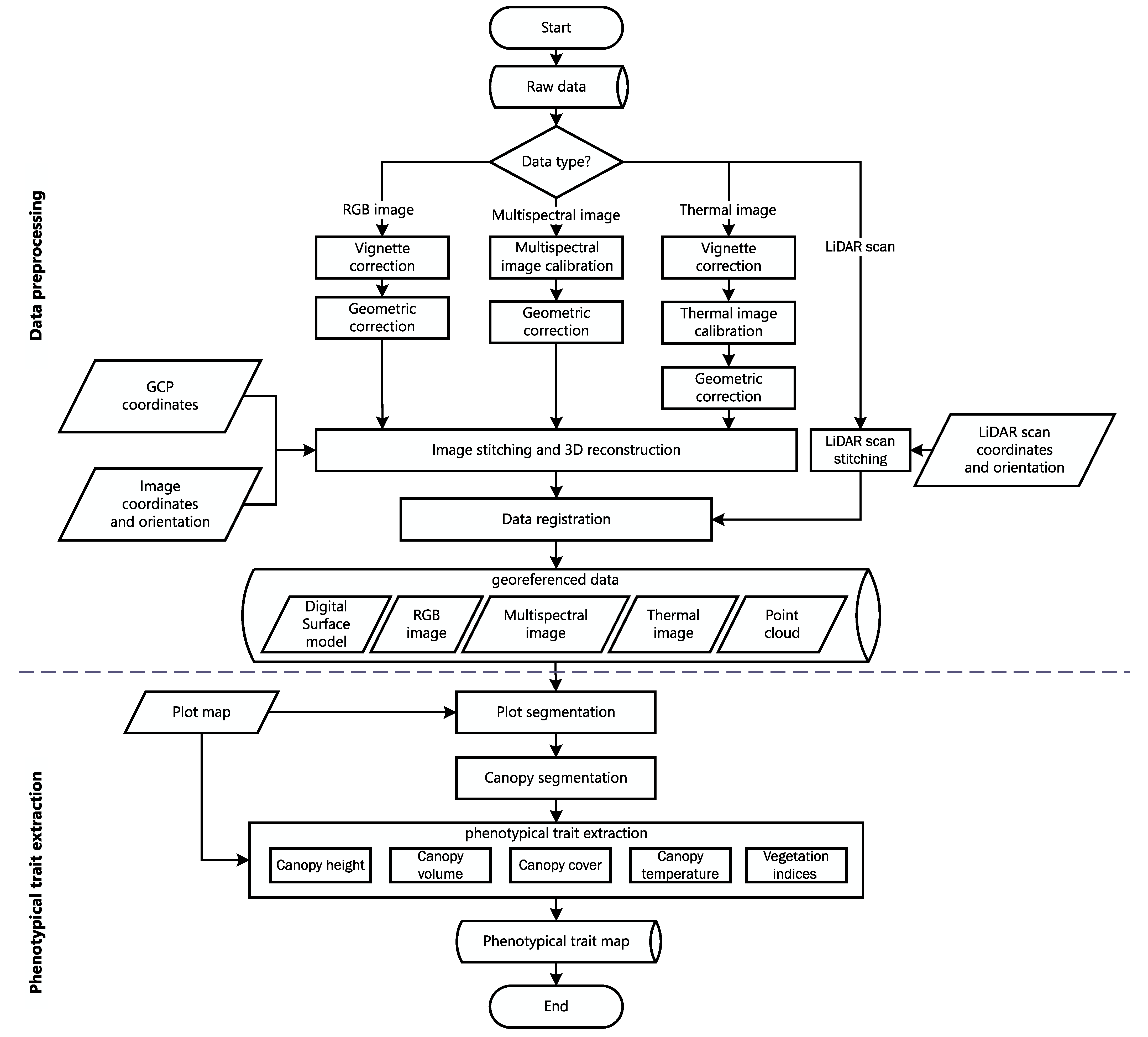
The data processing pipeline includes data preprocessing and phenotypic traits extraction (Figure 6). Data preprocessing calibrates images, generates georeferenced orthomosaics, and creates 3D models. Several phenotypic traits can be extracted using the preprocessed data, including canopy morphological traits, canopy vegetation index, and canopy temperature. Data preprocessing can partially be performed by the computer onboard the UAV in real time, which helps with field decisions and coordination with personnel and ground robots. We implemented software for online image geometric correction for the thermal and RGB images. We used Metashape (Metashape Professional 1.6.4, Agisoft, St. Petersburg, Russia) and Python to process images offline.

4.2. Data Preprocessing

4.2.1. Vignetting Correction

Vignetting correction was performed using the vignetting model obtained from the vignetting calibration. The corrected image intensity ( I c o r r e c t e d ) is calculated using Equation (5) from the original image intensity (I), the sensor black-level (BL), and the vignetting correction factor (V) [37]. For the multispectral image, the vignetting correction is integrated as a part of the radiometric calibration.
I c o r r e c t e d ( x , y ) = I ( x , y ) B L ( x , y ) V ( x , y )

4.2.2. Geometric Correction

The geometric correction was performed using the coefficients of the lens distortion model obtained from the geometric calibration. For the RGB and the thermal cameras, we used the image_geometry package coded in the ROS nodes. The calibrated images were published as rgb/rect_image and flir_tau2/rect_image topics.

4.2.3. Multispectral Image Calibration

Raw multispectral images were processed to compute reflectance of ground objects. Processing included three steps: radiometric calibration, sunlight intensity correction, and reflectance calculation. Radiometric calibration was used to convert raw digital values of the multispectral image to absolute spectral radiances. The radiometric calibration model provided by MicaSense (https://support.micasense.com/hc/en-us/articles/115000351194-RedEdge-Camera-Radiometric-Calibration-Model, accessed on 1 October 2020) was used to compensate for sensor black level, the sensitivity of the sensor, sensor gain and exposure settings, and optical vignetting effects (Equation (6)):
L ( x , y ) = 1 V ( x , y ) · a 1 g · p ( x , y ) p B L t e + a 2 y a 3 t e y
where L is the absolute spectral radiance value in W m 2 sr 1 nm 1 , V is the correction factor from the vignetting model, p is the normalized raw pixel value, p B L is the normalized black level value, a 1 to a 3 are the radiometric calibration coefficients that can be obtained from the image metadata, t e is the image exposure time, g is the sensor gain setting, y is the row number, and ( x , y ) is the pixel position.
After radiometric calibration, radiance values for each multispectral image were corrected against incident sunlight; thus, radiance values from different images represent the same illumination conditions. The intensity of the sunlight was measured using the downwelling light sensor provided by MicaSense.
In order to account for changes in illumination during flights, a calibrated reflectance panel (MicaSense, Seattle, WA, USA) was imaged before and after each flight. Average values of radiance for pixels collected over the panel area were then linearly interpolated over time to compute a reflectance calibration factor for each spectral band. In order to compute reflectance bands, radiometrically calibrated bands representing radiance values were multiplied by reflectance calibration factors. Following the implementation of image calibration procedures in Metashape, we directly used Metashape’s reflectance calibration function to compute reflectance.

4.2.4. Thermal Image Calibration

The accuracy of temperature values derived from thermal images largely depends on how much environmental effects during acquisition can be compensated using image processing. In particular, environmental effects can be significant when objects are far from the camera and when atmospheric contributions increase.
According to the Stefan–Boltzmann law, the total radiation emitted by the object is expressed as Equation (7):
B ( T ) = ε · σ · T 4
where ε is the emissivity, and σ is the Stefan–Boltzmann constant ( 5.67 × 10 8   W m 2 K 4 ). T is the absolute temperature (K).
The total radiation received by the thermal camera ( W s e n s o r ) consists of emission of the object ( E o b j ), the emission of the surroundings and reflected by the object ( E r e f l ), and the emission of the atmosphere ( E a t m ) (Equation (8)) [39].
W s e n s o r = E o b j + E r e f l + E a t m
W s e n s o r can be expressed as follows:
W s e n s o r = σ · T s e n s o r 4
where T s e n s o r is the apparent temperature provided by the thermal camera by setting the emissivity of the object to 1 and distance to 0.
Since the surface radiance is received partially by the camera and some is absorbed by the atmosphere, E o b j can be expressed as Equation (10) as a function of the transmittance of the atmosphere ( τ ) and the object’s temperature ( T o b j ).
E o b j = τ · ε · σ · T o b j 4
E r e f l is the reflected radiation of the surroundings (which is the downwelling atmosphere radiation), and it is partly absorbed by the atmosphere. Thus, E r e f l can be expressed as the following equation using the reflected apparent temperature ( T r e f l ),
E r e f l = τ · ( 1 ε ) · σ · T r e f l 4
E a t m is the emission of the atmosphere that reaches the thermal camera, which is the upwelling atmosphere radiation. It can be expressed as the following equation:
E a t m = ε a t m · σ · T a t m 4 = ( 1 τ ) · σ · T a t m 4
where T a t m is the temperature of the atmosphere (air temperature), and ( 1 τ ) is the emissivity of the atmosphere.
Equation (13) can be used to retrieve the temperature of the object and results from combining Equations (8)–(12).
T o b j = T s e n s o r 4 τ · ( 1 ε ) · T r e f l 4 ( 1 τ ) · T a t m 4 τ · ε 4
In order to solve Equation (13), the transmittance of the atmosphere, the emissivity of the object, the air temperature, and the reflected apparent temperature need to be supplied. The air temperature can be measured by a temperature sensor. The reflected apparent temperature can be indirectly measured by measuring the apparent temperature of an aluminum plate or directly measured by measuring the sky’s apparent temperature using an infrared thermometer.
The transmittance of the atmosphere ( τ ) is estimated using the water vapor content (WVC) and flight height above the ground (distance) with the following equation [40]:
τ = K a t m · exp d α 1 + β 1 ω + ( 1 K a t m ) · exp d α 2 + β 2 ω
where ω is the water vapor content (mm), d is the distance (m), and K a t m = 1.9 is the scale factor of atmospheric damping. α 1 = 0.0066 and α 2 = 0.00126 are the attenuation of the atmosphere without water vapor, and β 1 = 0.0023 and β 2 = 0.0067 are the attenuation of water vapor. The WVC can be estimated using the air temperature and humidity using the following equation [40]:
ω = ω % · exp h 1 · T a 3 + h 2 · T a 2 + h 3 · T a + h 4
where ω % is the relative humidity (ranging from 0 to 1; dimensionless), T a is the air temperature (°C), h 1 = 6.8455 × 10 7 , h 2 = 2.7816 × 10 4 , h 3 = 6.939 × 10 2 , and h 4 = 1.558 [40].
It has been reported that the emissivity of vegetation ranges from 0.96 to 0.99, while the emissivity of soils is around 0.98 [41,42]. The inaccuracy in emissivity can result in temperature errors of up to several degrees Celsius [43], and in this study we estimated emissivity of vegetation canopy and soil using the Normalized Difference Vegetation Index (NDVI), as proposed by [44].
The contribution of E r e f l and E a t m to W s e n s o r is different under different atmospheric conditions. Equations (14) and (15) show that higher air temperatures, humidity, and flight altitude result in lower transmittance of the atmosphere, which makes E a t m contribute more to W o b j . In other words, the error of T a t m contributes more to the error of T o b j at lower atmospheric transmittance. T r e f l contributes more when the object has lower emissivity, which means that the error of T r e f l has more effect on the error of T o b j for objects with lower emissivity. Since vegetation and soil have emissivity close to one, the effect of E r e f l is small relative to the measurement of their real temperature.
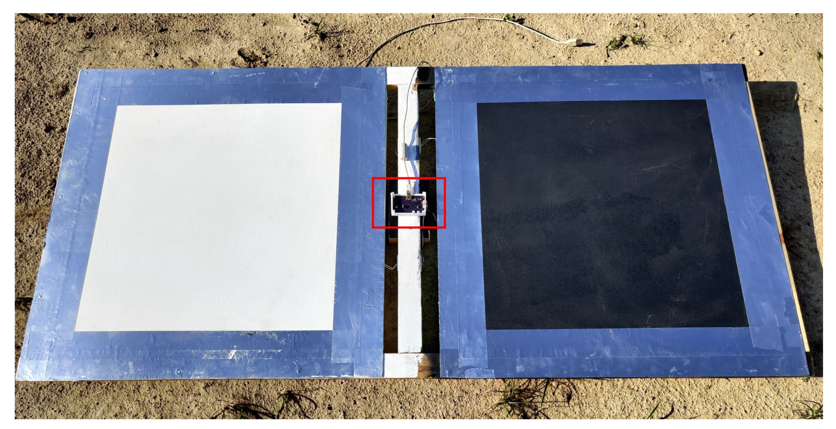
In order to assist the thermal calibration and validate temperature estimates, we made two thermal calibration targets and a customized device to record atmospheric conditions, including air temperature, air pressure, and humidity (Figure 7). Similar to other studies, the calibration target was made from a 0.6   m × 0.6   m aluminum plate for which its top surface was painted using flat paint, and the back was covered by polystyrene insulation foam [35]. The edge of the plate was wrapped with aluminum tape to assist auto-detection of the target. One target was painted in white to create a low-temperature reference (cold target), and the other target was painted in black to create a high-temperature reference (hot target). The top surface temperature of the targets was measured by a resistance temperature detector (RTD) (700-102AAB-B00, Honeywell, NC, USA) attached to the back of the aluminum plate. Emissivity calculation used the reference temperature method [43], and emissivities were 0.968 (white paint) and 0.984 (black paint). A thermal camera pointing upward was used to measure the reflected temperature. All ground measurements can be transmitted to the DAS through xBee in real time and be used to calibrate the thermal images.

4.2.5. LiDAR Data Processing

LiDAR scans can be assembled into point clouds using the scans’ position and pose in the East North Up (ENU) frame. RTK-GNSS or PPK-GNSS and IMU should be used to measure the accurate position and posing of the platform/sensor; thus, LiDAR scans can be assembled accurately. Since the current UAS does not have an RTK-GNSS and IMU, the LiDAR data were not used in this study. However, the LiDAR data processing was integrated as part of the overall data processing pipeline and is ready for the additional positional and attitude data, for example, by using an RTK-GNSS and IMU to obtain the precise location and orientation of each LiDAR scan [45].

4.2.6. Orthomosaics and 3D Model

Agisoft Metashape and Structure from Motion (SfM) techniques were used to process RGB images collected by individual UAS flights and to generate orthomosaics, 3D point clouds, and digital surface models (DSM) for each camera.

4.2.7. Data Registration

Data registration includes the registration of the orthomosaics from different cameras and the registration of the orthomosaics and the LiDAR data. In this project, the registration of orthomosaics is based on positional information stored with those products, including coordinates, spatial resolution, and projection. The accuracy of the registration will depend on the quality of this information and should increase when high-accuracy GNSS and ground control points (GCPs) are incorporated into data acqusition and processing.
Since different orthomosaics have different ground sampling distances (GSD), pixel-wise registration between two orthomosaics requires resampling one orthomosaic to a larger or smaller GSD in order to match the orthomosaic being used as reference. If differences in spatial resolution are considerable, downsampling to a coarser GSD can involve substantial loss of information. Conversely, upsampling can introduce unrealistic representations of detail to a scene. Considering the characteristics of the cameras incorporated into our system, for pixel-wise registration, higher-resolution orthomosaics (those derived from RGB images) were downsampled to spatially match the lower-resolution thermal orthomosaics.

4.3. Extraction of Phenotypic Traits

Multiple phenotypic traits can be extracted from data captured by the integrated cameras and LiDAR sensor. Basic traits can be extracted directly following data preprocessing, including vegetation indices (VI) derived from multispectral images and canopy temperature (CT) derived from thermal images, as well as morphological traits such as canopy height (CH), canopy cover (CC), and canopy volume (CV). More complex traits, such as biomass and water stress, are out of the scope of this paper but can be obtained from the basic traits using regression models [12,21]. A program was created to extract phenotypic traits automatically by using QGIS 3.10 and Python 3. The extracted traits were saved to a csv file and visualized in QGIS.

4.3.1. Plot Segmentation

Data collected for an entire field were partitioned into individual plots using a plot layout map. Data for each plot contained 2D images and a 3D model of the plot. Since each plot can be observed by several UAV images, a plot can have multiple plot images, including images extracted from the orthomosaics. Images from different view angles can provide additional information about the plot and can, for instance, support the detection of fruits and flowers [11].
The 3D model for each plot was normalized against the ground level to create a plot height model; thus, the height of data points represented the height above ground. A 2D plane representing the ground level can be found by fitting the plot model using the Maximum Likelihood Estimation Sample Consensus (MLESAC) [46]. If the plot model does not have enough ground points due to high canopy closure, the ground plane can be represented by a bare ground model or the Digital Elevation Model (DEM) collected before plants germinated [12]. In this case, additional data collection and accurate georegistration between the bare ground model and the plot model are required. Following estimation, the ground level was subtracted from the plot model to represent height above ground.

4.3.2. Canopy Segmentation

Each plot was segmented in order to isolate and extract canopy specific metrics representing phenotypic traits. The segmentation result is a canopy mask generated from the 2D plot image or a canopy model generated from the plot height model. Color, spectral, and height differences between the canopy and ground can be used for the segmentation [20]. In this study, the thresholding method was verified to adequately segment canopies by using an RGB image and the 3D model for the plot. Other methods, such as deep neural networks and including Mask R-CNN, may offer segmentation improvements but they are out of this paper’s scope.

4.3.3. Morphological Traits

Morphological traits are important phenotypic traits that are often related to plant growth status. For example, canopy height and volume can be used to quantify cotton biomass, which is correlated with yield. This work computed two morphological traits (canopy height and canopy volume) for each plot.

Canopy Height

Canopy height was calculated using the canopy model. Strategies for canopy height computation vary and some studies use an average or median canopy height to represent the height of the crop. This approach is suitable for crops whose canopy are evenly distributed, such as barley and wheat [12,16,47]. Other studies have used a percentile of the canopy height to represent the height of the canopy, which can reduce the effect of uneven distribution of the canopy [15,48]. This study used an exploratory approach and combined both strategies to calculate canopy height using the average, maximum, median, and 50th to 99th percentiles with a 10th interval.

Canopy Volume

The canopy model was used also to compute canopy volume, represented by the volume of the mesh that encloses the 3D canopy model. The mesh can be found using a convex hull algorithm. However, since canopy models generated by aerial images or LiDAR usually lack information below the canopy surface, computing volume directly from the mesh can underestimate the canopy. Instead, we proposed to calculate the 2.5D volume as the canopy volume. The canopy model was first converted to a depth image for which its intensity represented height, and then the 2.5D volume of the depth image was calculated using Equation (16):
C V = Δ x Δ y i j d i , j
where Δ x and Δ y are the ground sample distances, and d i , j is the depth of the pixel.

Canopy Cover

Canopy cover is defined as the ratio of the vertical projected area of the canopy to the area of the plot. After segmenting the canopy, the area of the canopy can be calculated as the ratio of the pixel area of the canopy mask to the pixel area of the plot.

4.3.4. Vegetation Indices

Multiple indices have been proposed in the literature to describe vegetation status and processes based on multispectral data [49]. In this paper, we characterized field plots by calculating one widely used vegetation indices: the Normalized Difference Vegetation Index (NDVI). For each plot, a representative vegetation index value was calculated by averaging all vegetation indices for the area covered by the canopy.

4.3.5. Canopy Temperature

Canopy temperature was calculated using values extracted from the thermal orthomosaic that correspond to each plot area. Similarly to the computation of vegetation indices, canopy temperature was calculated as the average temperature within the canopy for each individual plot.

5. Data Collection

5.1. Testing Field

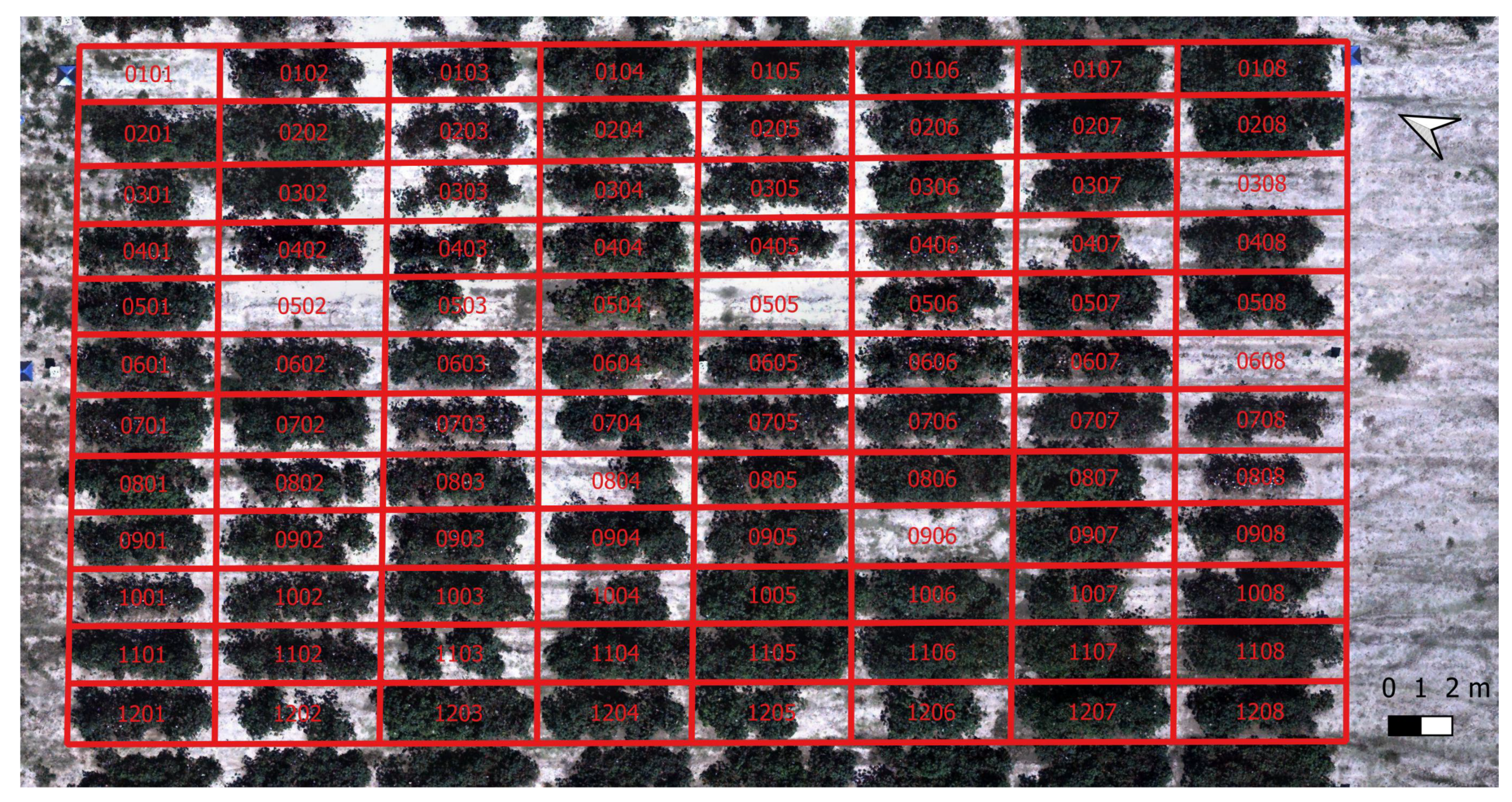
Tests of the data collection platform were conducted using a cotton field located on a university research farm in Watkinsville, Georgia, United States. The field comprised of 96 plots arranged in 8 columns and 12 rows (Figure 8). The length of each plot was approximately 3 m, and there was a 1.5 m long alley between the plots. The distance between the crop rows was 1.8 m.

5.2. GCP Deployment and Field Mapping

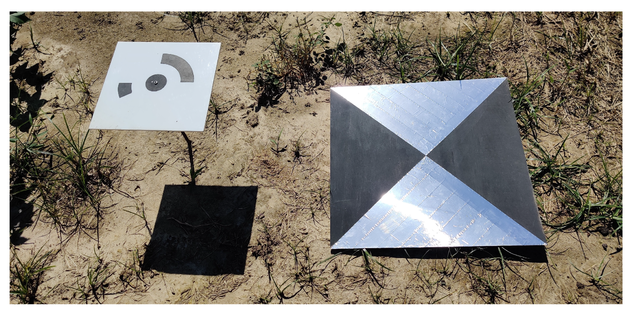
The testing field was prepared prior to data collection in order to facilitate collections throughout the growing season, as well as data processing and analyses in the office. First, in order to improve the accuracy of the georeferencing of the orthomosaic, ground control points (GCPs) were deployed in the field. GCPs were ground targets with known coordinates and that had a distinct pattern that allowed for easy identification in images. Some photogrammetry software, Metashape included, provide GCP patterns that can be identified automatically by the program. In this study, we made two types of GCPs: (a) GCP in black and white for RGB and multispectral cameras and (b) GCP for thermal camera. For the RGB and multispectral cameras, we used 12-bit circular coded targets generated by Metashape as GCP patterns (Figure 9). The patterns were made of black vinyl sheet and pasted onto a white acrylic panel. The size of the acrylic panel was 0.6   m × 0.6   m , and the center point radius of the circular coded target was 30 mm. GCPs for the thermal camera were made of 0.8   m × 0.8   m wood panels. The panels were evenly divided into four quadrants with two opposite quadrants painted in black and the other two covered by aluminum tape (Figure 9). Due to the distinct emissivities of the black paint and aluminum, GCPs for the thermal camera could be easily identified in thermal images. For our test field, we used nine GCPs for the RGB and multispectral collections, and the GCPs were fixed in the field throughout the growing season. The GCPs were raised above the ground to avoid being covered by the weeds and plants. Coordinates for those GCPs were measured periodically over the season using an RTK-GNSS to account for unintended movement of GCPs by farm operations during the season. For the thermal collections, we used six GCPs, which were deployed in the field during UAV operations as the GCPs were not weather proof. Coordinates for the thermal GCPs were obtained from the georeferenced RGB orthomosaic.
In addition to GCP deployment, we conducted a flight prior to plant emergence to map the testing field. Pre-collection mapping of a field site was a key step of our workflow and supports data processing by the following: (a) producing a plot layout map used for plot segmentation and (b) allowing for the generation of a bare ground model. Field mapping was performed one week after planting.

5.3. Flight Path Planning

Most UAVs are equipped with autopilot and can fly planned flight paths. To plan our flights, we paid particular attention to flight height above ground and percentage of image overlap. Flight height affects the ground resolution of aerial images and the size of image footprints. Image overlap (forward and side overlap) affects the quality of image stitching and 3D reconstruction, being a function of flight height, flight speed, image recording frequency, and flight path configuration. Within the same flight path, lower flight height, faster flight speed, and/or lower image recording frequency results in lower forward overlap. Conversely, higher forward overlap can be obtained by increasing flight height, by reducing flight speed, and/or by increasing image recording frequency. Side overlap can be increased by increasing flight height and/or by reducing the distance between flight lines. In addition, image overlap can be increased by using a cross-stitch flight pattern [50].
Lower flight height and higher image overlap can effectively increase image resolution and the quality of image stitching and 3D reconstruction. On the other hand, these settings increase flight time and result in a larger number of images being collected, which increases data processing time. Considering the above, we proposed a general multi-step decision-making process to balance flight height, flight speed, and image overlap. First, we selected the appropriate flight height based on the desired aerial image resolution. Second, we define the side overlap percentage. One study suggested that side overlap should be at least 67% to obtain complete 3D reconstruction for forest [51]. Based on our experience, a good range of side overlap is 70% to 80% considering flight time, area coverage, and processing time. Following the definition of flight height and side overlap, a flight path can be generated. The final step is to decide the forward overlap and flight speed. Higher forward overlap can result in more complete and better quality 3D reconstructions [51]. We suggest a forward overlap from 80% to 90%. Flight speed is defined considering that the camera should not move more than half the Ground Sampling Distance (GSD) during exposure to avoid motion blur. As a result, flight speed should be smaller than p h 2 T e f , where p is the pixel pitch, h is the flight height, T e is the exposure time, and f is the focal length. For example, the flight speed for the RGB camera used by our system should not exceed 8 m / s at 25 m flight height and 1 m s exposure time. A higher flight speed can be used with a smaller exposure time without increasing the flight height (or GSD) and creating blurry image.

5.4. Flight Campaign

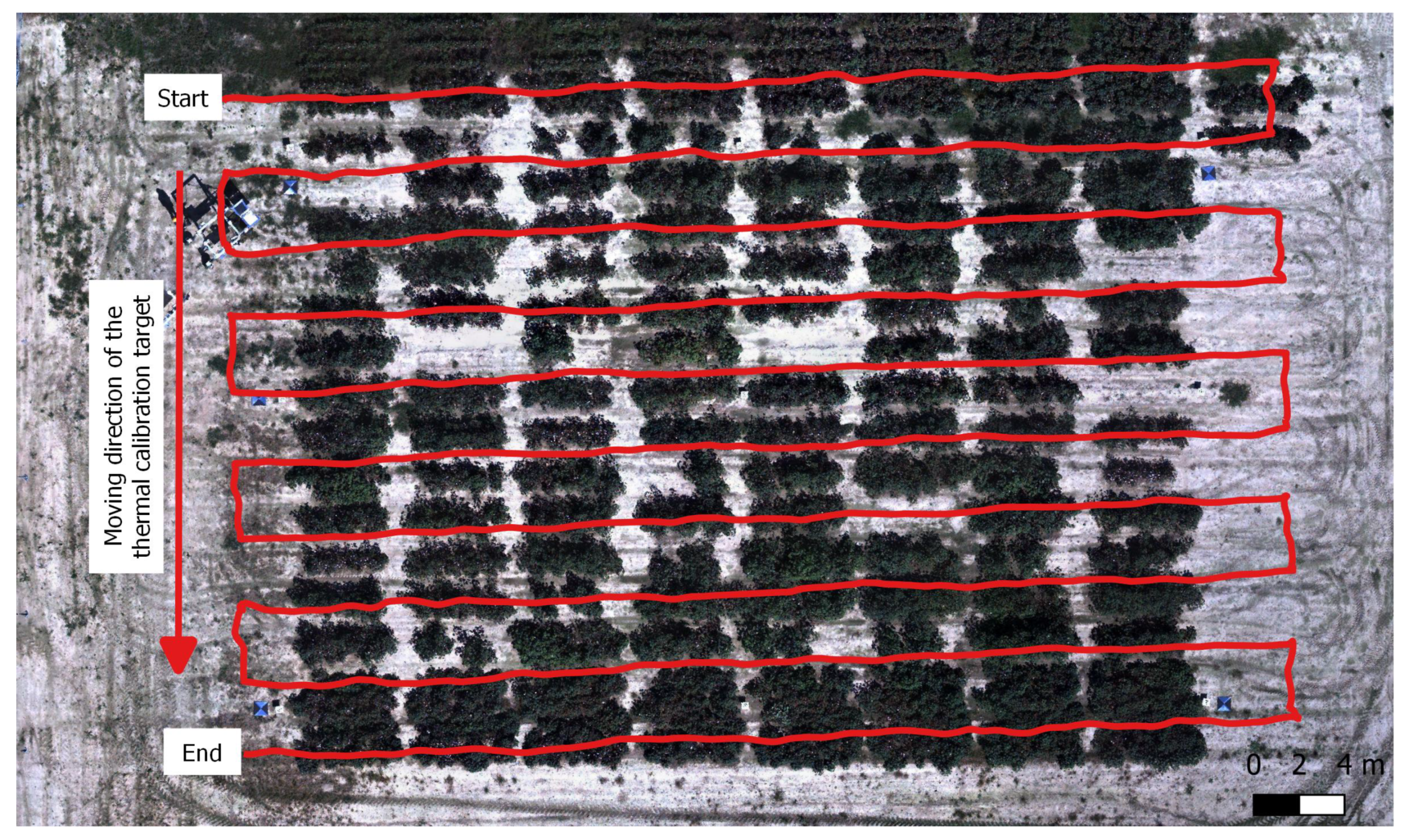
A DJI Matrice 600 equipped with the second version of the DAS was used for data collection. Pixel4Dmapper was used to generate the flight path and control the UAV. The flight path was generated considering a 25 m flight height above the ground, 70% side overlap, and 90% forward overlap (Figure 10). The speed of the drone was set at 1 m/s. The flight path was calculated based on the specifications of the thermal camera, considering that camera has the smallest field of view among all the cameras used. This choice resulted in higher image overlap for the RGB and multispectral cameras. Due to the DJI Manifold’s limited data saving speed, the camera triggering frequency was set to 0.5   Hz to avoid data loss, although both the RGB and the thermal cameras support much higher trigger frequency.
The flight campaign was performed on 1 October 2020 at 2:30 p.m. The weather was sunny, with an average wind speed of 1.5 m/s. The reflectance target for the multispectral camera was imaged before and after the flight. The thermal calibration targets were mounted on a mobile robot that moved along the west border of the field so that the thermal calibration targets could be imaged multiple times by the thermal camera during the flight (Figure 10). The thermal calibration targets were imaged nine times during the collection.

5.5. Ground Data Collection

Ground data were manually collected for one crop row in the field simultaneously to the flight campaign and were used as reference to validate the extracted traits from images. The height of each plant was manually measured by using a ruler, and the average canopy height and maximum canopy height were then calculated for each plot as the average and maximum height of the plants within the plot. Ground measurements of NDVI used a handheld NDVI sensor (GreenSeeker, Trimble, Sunnyvale, CA, USA) and we calculated canopy NDVI for each plot as the average of four NDVI measurements conducted at different locations inside the plot. Temperature measured by the thermal calibration targets was used as ground reference for the targets’ surface temperature and was compared with the temperature measured by the thermal camera. Similarly, canopy height and canopy NDVI resulting from manual measurements were compared to corresponding values derived from aerial images. The mean absolute error (MAE) (Equation (17)) and mean relative error (MRE) (Equation (18)) were used to evaluate deviations from measurements (ground reference).
MAE = 1 N i = 1 N UAV derived i ground reference i
MRE = 1 N i = 1 N UAV derived i ground reference i ground reference i

6. Results

6.1. Camera Calibration

6.1.1. Camera Geometric Distortion

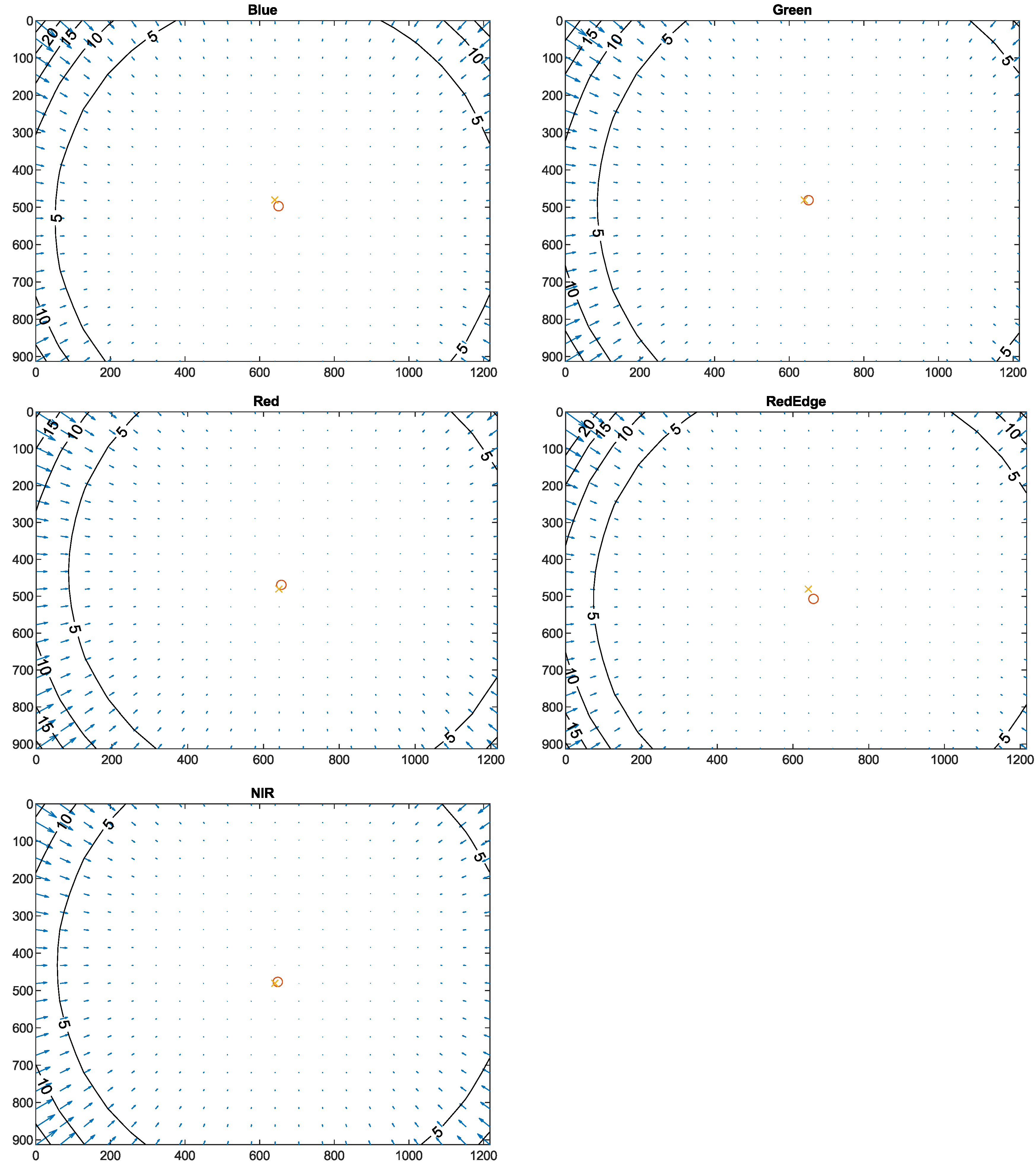
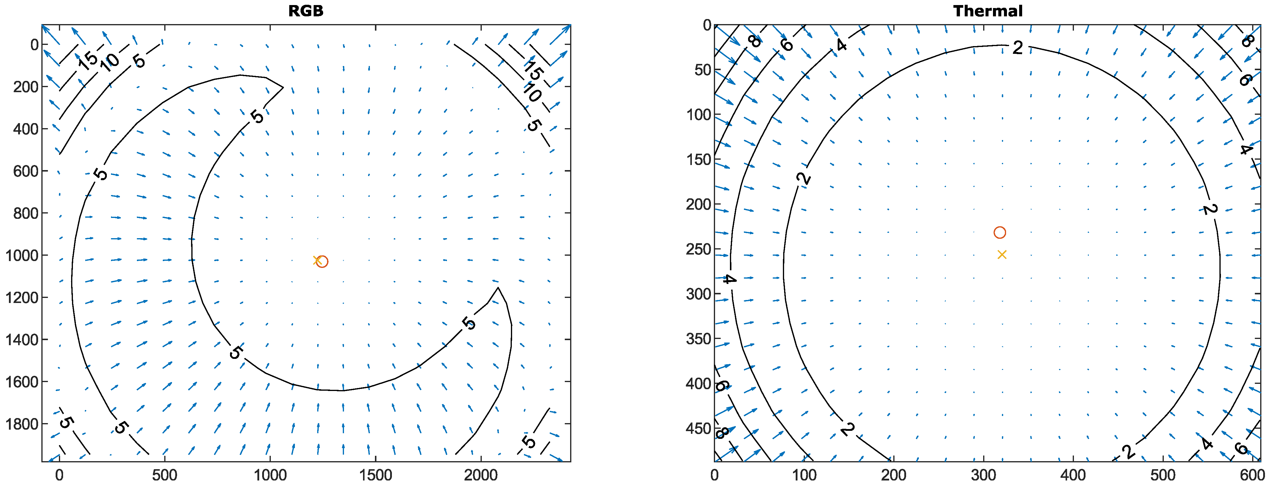
Table 2 shows the cameras’ intrinsic parameters and the parameters of the distortion models. The multispectral camera’s nominal focal length is 5.4 mm, but the focal lengths over the five bands ranged from 5.469 mm in the red band to 5.513 mm in the green band. The RGB camera’s and the thermal camera’s focal lengths are very close to their nominal focal length (5 mm and 25 mm, respectively). For the multispectral camera, the NIR band has the largest offset of the principal point from the origin (central pixel). The thermal camera’s principal point also has a large offset from the origin in the y-axis. The total distortion (combination of radial and tangential distortions) of the three cameras is shown by Figure 11 and Figure 12. The three cameras have low distortion, and the distortion is only noticeable near the border of the image.
In practice, camera distortion optimization is usually part of the bulk bundle adjustment of the photogrammetry process for image stitching and 3D reconstruction. Thus, it is unnecessary to perform the correction separately. However, the model parameters in Table 2 can be used as initial values for the camera distortion optimization in the photogrammetry process.

6.1.2. Camera Vignetting

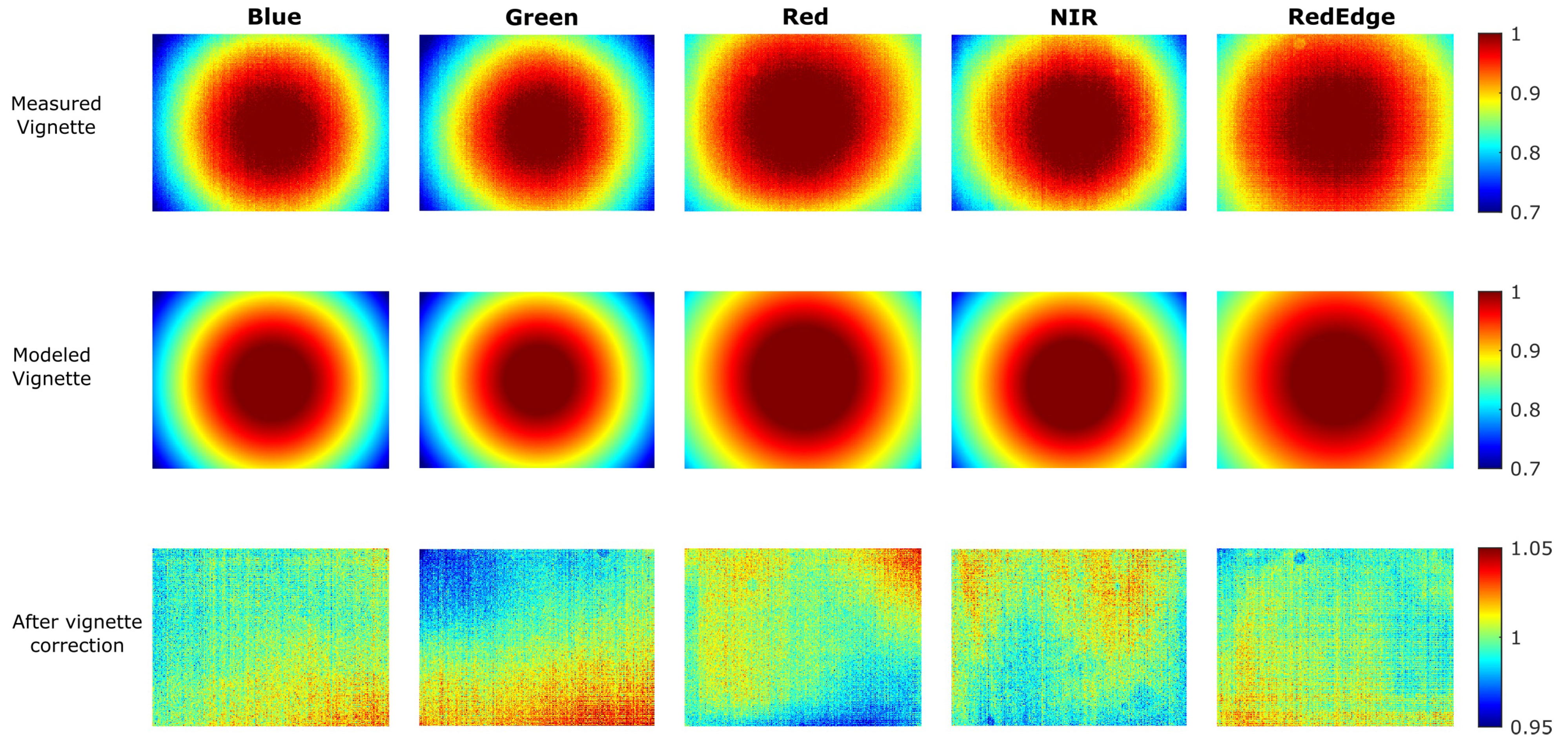
Figure 13 shows vignetting for images collected by the multispectral camera, where image centers are brighter than borders. Measured and modeled vignette show that each image band is affected differently by vignetting, as a function of their individual lens system and aperture. The correction of vignetting is, thus, conducted on a per-band basis, and the results of vignette correction are also shown by Figure 13.
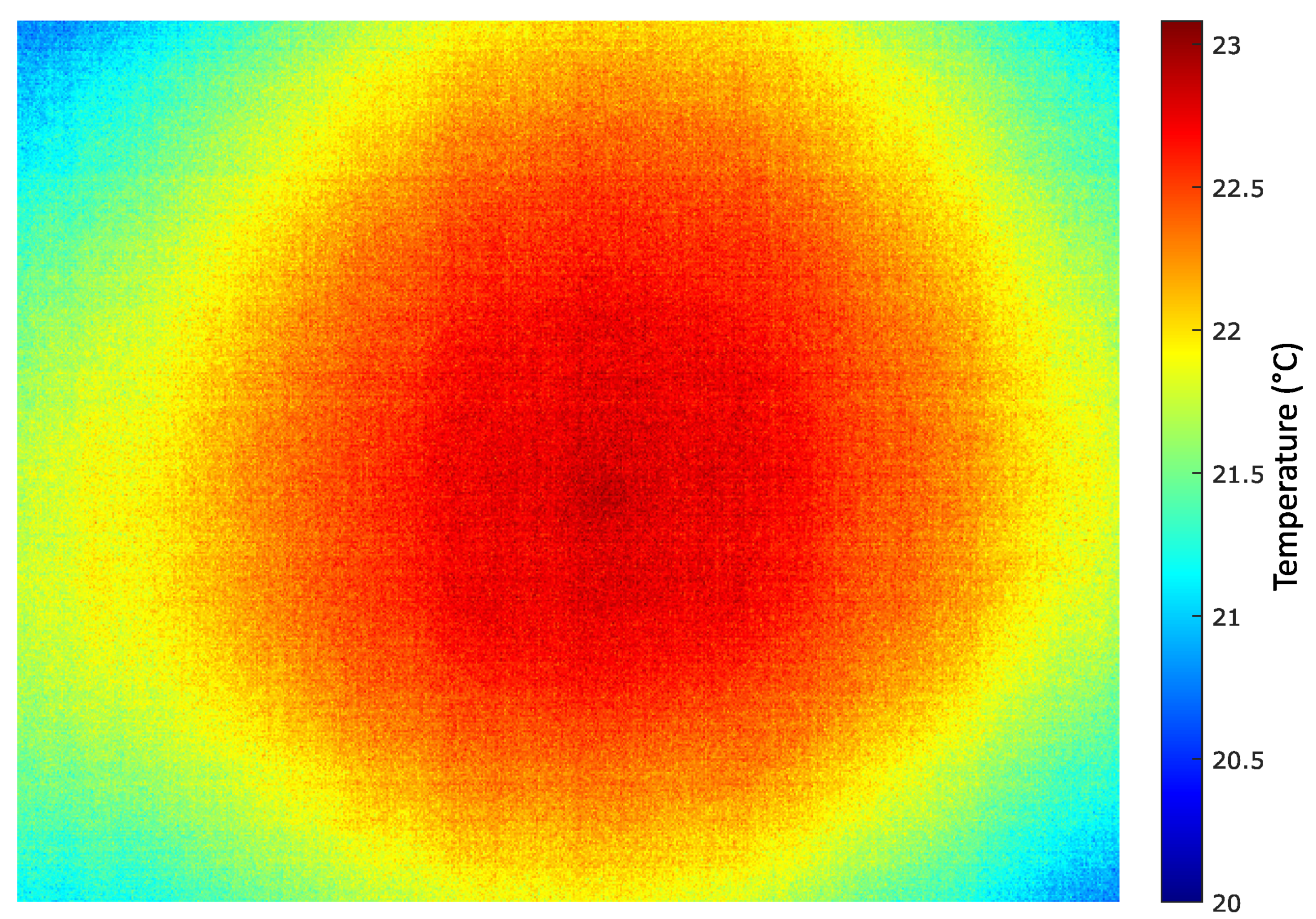
The vignetting pattern for the thermal camera was comparable to the pattern observed for the multispectral camera (Figure 14). However, unlike the multispectral camera, for which vignetting mainly results from optical properties of the lens, the vignetting of an uncooled thermal camera can be caused by differences in response to irradiance by each detector element, which depends on ambient temperature and the temperature of the detector. To address vignetting of thermal images, multiple vignetting correction models need to be created for different ambient temperatures. Effects of vignetting on temperature estimates for pixels near the edge of images can be significant, as temperature for those pixels can be offset by up to 3 °C [52]. In this study, we did not perform vignetting correction for the thermal camera. Instead, we discarded pixels close to edges and measured temperature by using only the central portion of images (within a distance of 100 pixels from the optical center). A more thorough study addressing corrections of vignetting effect for the thermal camera is planned for future work.

6.2. Data Preprocessing

6.2.1. Accuracy of the Thermal Camera Calibration

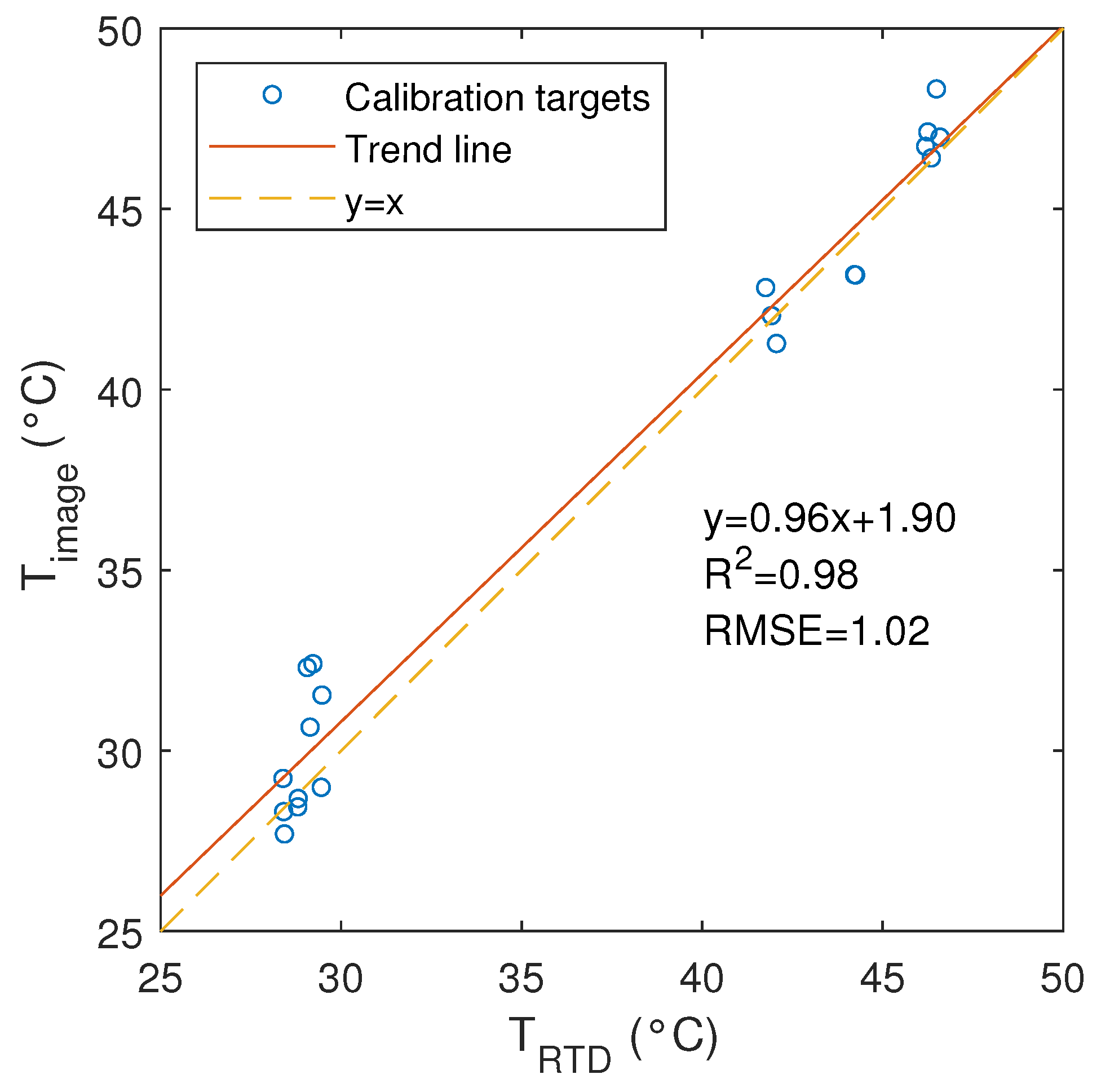
During the data collection flight, the air temperature and humidity varied from 28.3 °C to 31.7 °C and from 35.7% to 40.5%, respectively (Figure 15). Conditions resulted in high transmittance of the atmosphere ( m e a n = 0.9249 , s t a n d a r d d e v i a t i o n = 0.0011 ) and resulted in little impact of upwelling atmosphere radiation on thermal images. After image calibration, temperatures of the two calibration targets derived from thermal images were highly correlated with temperatures measured by the RTD sensor, and pre-calibration MAE ( 6.62 °C) was significantly reduced to 1.02 °C (Figure 16).

6.2.2. Results of Orthomosaic Generation

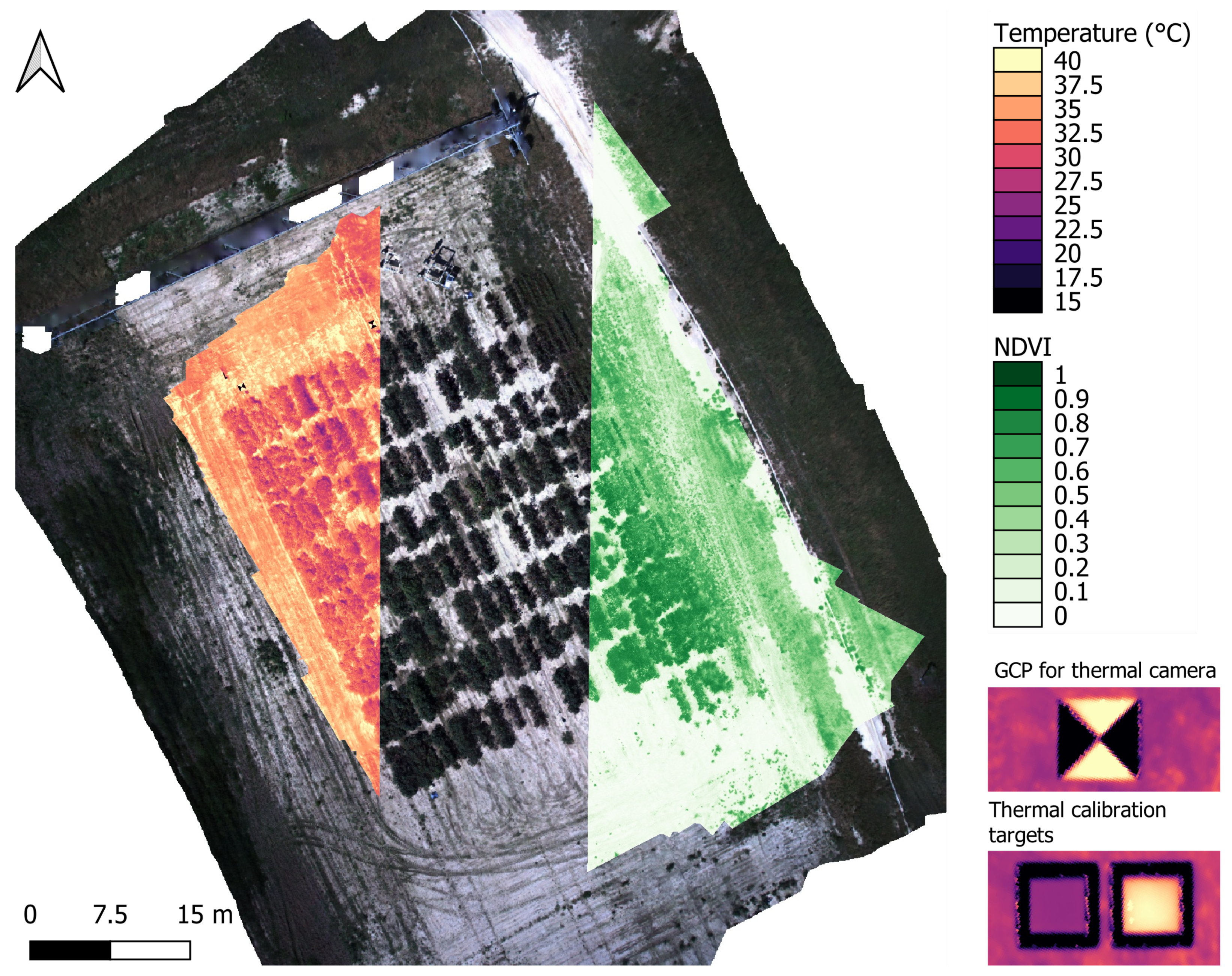
We used GCPs and image locations provided by the UAV as input to Metashape to successfully generate georeferenced orthomosaics for RGB, multispectral, and thermal images (Figure 17). In order to ensure adequate spatial resolution and to facilitate overlay and comparisons, the GSDs of processing outputs were set to 0.016 m for all cameras. The RGB camera had the largest FOV, followed by the multispectral camera and the thermal camera. Resulting from the larger FOV of the RGB camera, the RGB orthomosaic had the largest ground coverage and included areas outside the cotton field. When preparing flights, the FOV of the RGB camera can be reduced by increasing the camera’s focal length. This results in reduced GSD without losing the coverage of the field.

6.3. Phenotypic Traits Extraction

6.3.1. Results of the Canopy Segmentation

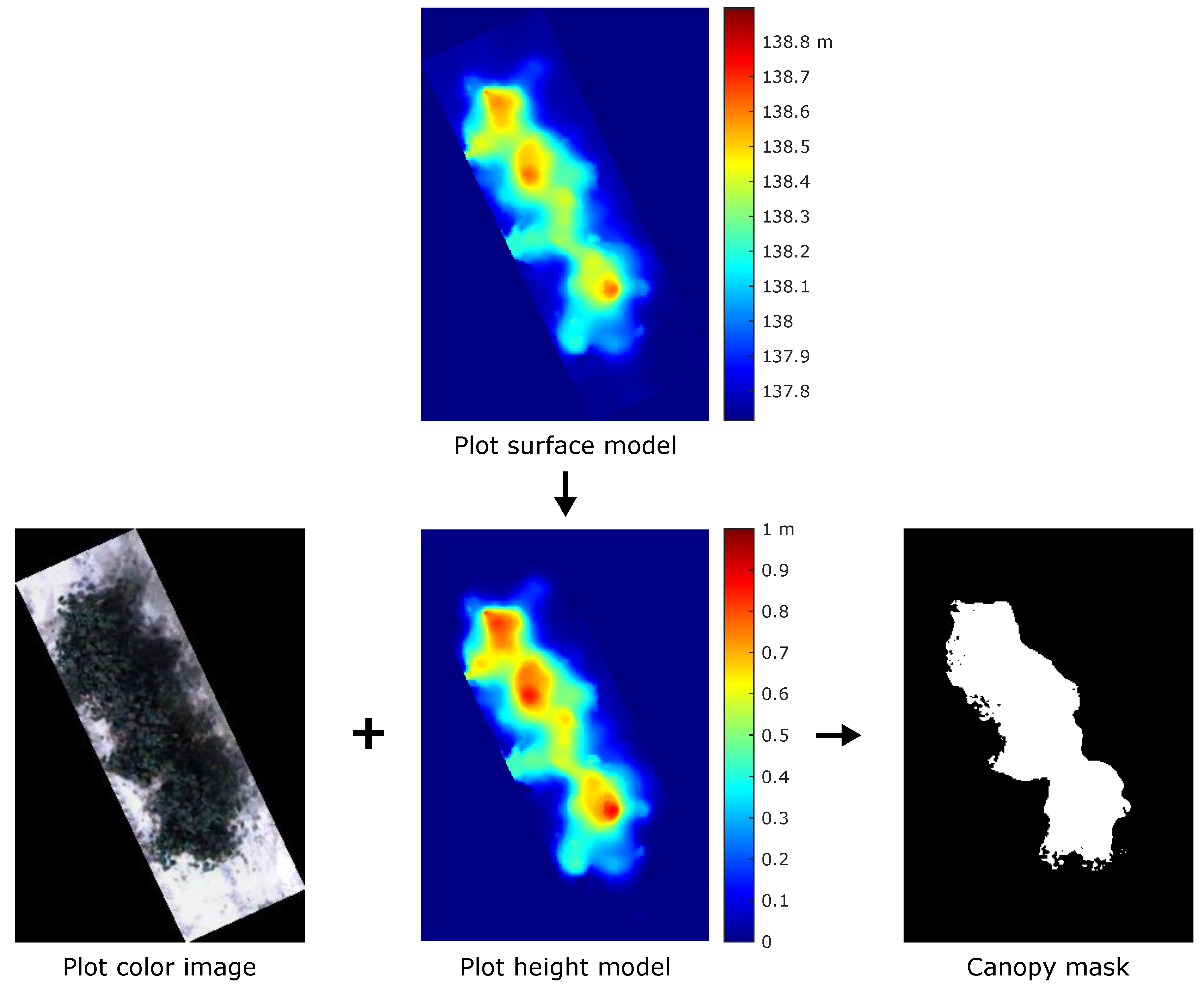
The performance of canopy segmentation is key to the extraction of phenotypic traits that depend on the number, size, and location of segments in order to calculate plant and ground cover metrics. Considering the significant differences in color between canopies and soil at the field site, a simple thresholding method was able to segment canopies and to create canopy masks efficiently (Figure 18). For crops with a large canopy, such as cotton, the plot height model can be used to refine results and to remove weeds that are lower than a threshold ( 0.2 m for this study).

6.3.2. Accuracy of the Canopy Height

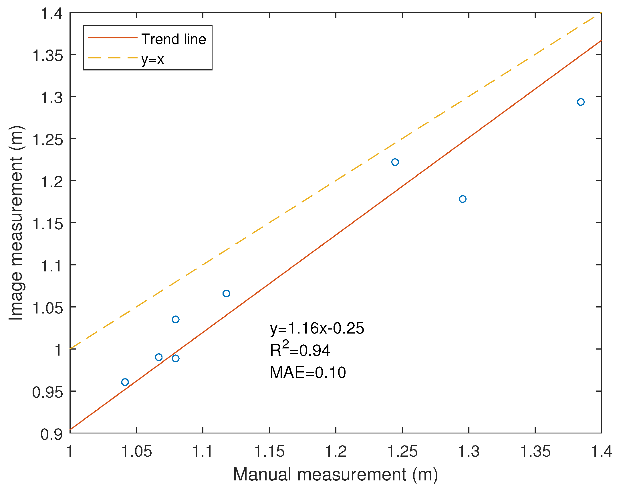
Canopy height values derived from RGB images were highly correlated with manual measurements. The MAE of maximum canopy height derived from images was 0.1 m and the majority of UAV-based measurements were lower than manual measurements. This is consistent with other studies in which the error associated with canopy height estimates based on photogrammetric methods is within the range of 0.07 m to 0.1 m (Figure 19) [15,16,20]. Errors linked to canopy height estimates largely depend on the accuracy of the DSM, which is affected by the spatial resolution of images. Incorrect detection of the ground plane can also result in large errors when generating the plot height model and can usually occur under close canopy and little ground exposure. In this case, the bare ground model should be used to define the ground plane. Other environmental factors, such as plant movement because of wind, also contribute to increased error.
The 99th percentile canopy height had the smallest MAE compared with the average of manually measured canopy heights (Table 3), but the median canopy height had the largest coefficient of determination. It is hard to conclude which statistical metric can better represent the true plot-level canopy height with such a small validation dataset. The choice of metric can be dependent on the type of crop being analyzed and should be determined experimentally by collecting validation data in the field.

6.3.3. Accuracy of the Canopy Vegetation Index

The image-extracted canopy NDVI had an MAE of 0.0518 with an MRA of 6.6% compared with the ground-measured NDVI. Results show that our workflow can derive accurate computations of this vegetation index. Other studies have confirmed that the MicaSense RedEdge camera was able to provide accurate NDVI measurements when compared to the GreenSeeker sensor [53]. It is noteworthy that multispectral images can reveal NDVI variations within the canopy, which can be an advantage over point-based sensors with limited FOVs.

6.3.4. Data Visualization

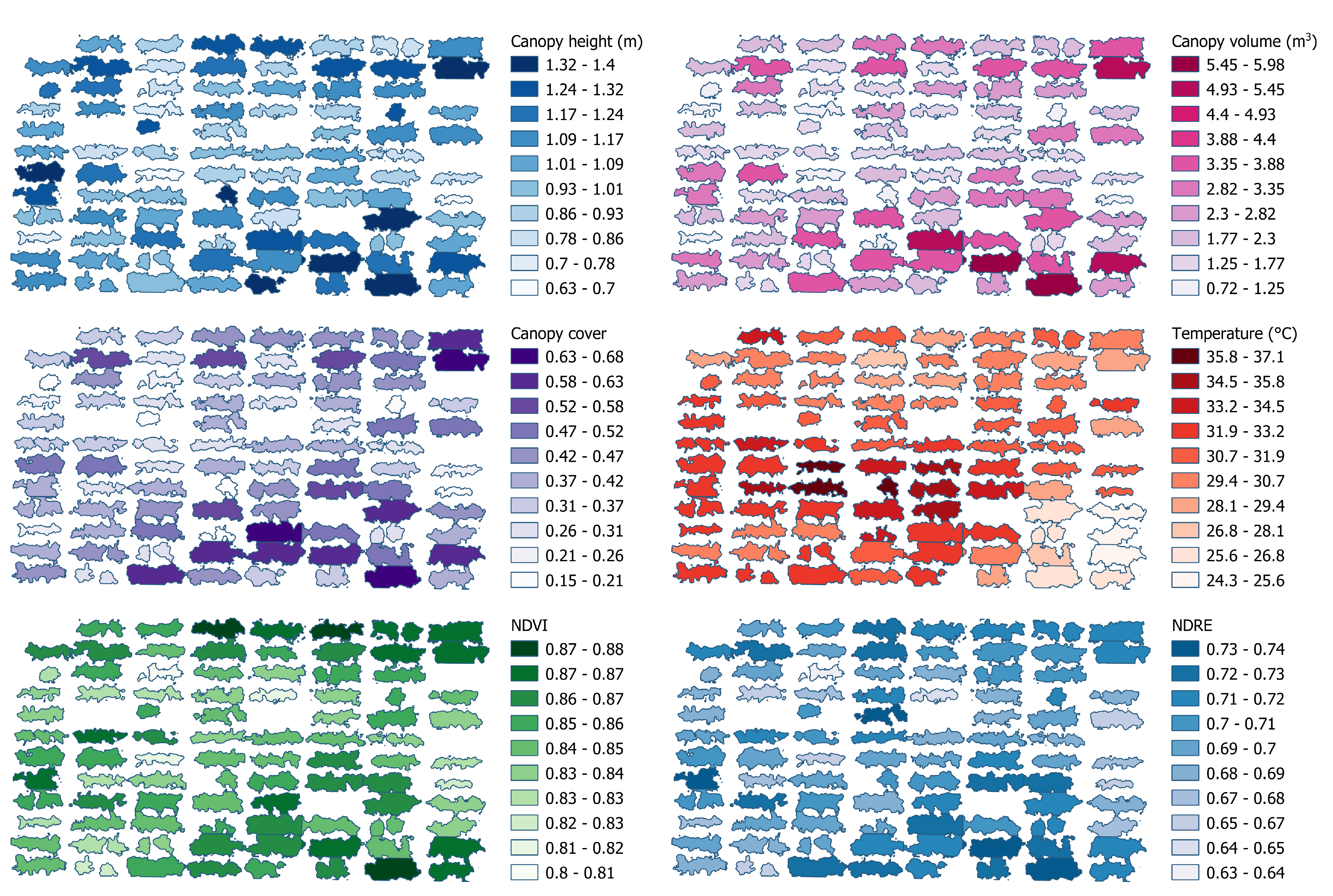
The extracted phenotypic traits were visualized in QGIS (Figure 20), where polygons delineate individual plots, and the shade of a color represents a range of values for a given metric or trait. For instance, those plots with lower vegetation correspond to lower NDVI and NDRE and higher canopy temperature. The visualization is helpful for researchers to examine the spatial distribution of the data and to present the results to the general audience. It also supports interplot comparisons and analyses with other co-located data, such as those associated with irrigation or use of fertilizers.

7. Discussion

UAVs have been used widely for plant phenotyping, and the literature shows a variety of platforms being used for the calculation of biophysical descriptors based on RGB, thermal, and multispectral cameras. In general, a multi-sensor system is able to collect more feature-rich data and derive more complex phenotypic traits than a single sensor. For example, cotton yield can be estimated more accurately using multiple features extracted from RGB, multispectral, and thermal images than a single image feature extracted from a single camera [54]. Different types of sensors can provide complementary information to improve the accuracy of phenotypic trait extraction. For example, high-resolution RGB images can support more detailed segmentation of canopies and can more accurately guide the calculation of canopy temperature from low-resolution thermal images. The downside of multi-sensor systems is the relatively higher payload requirement when UAVs need to carry multiple sensors simultaneously. Compared to existing UAV systems, our system was designed to allow for system customization, considering the need for flexible payload configurations based on study requirements and potential budget limitations. Each sensor can be attached to or detached from the UAV system as needed. Our system is not tied to specific crops and can be used for different fields including row crops and vineyard, with no specific requirement for the field layout (e.g., row spacing). For example, the UAS can be used to collect multispectral image to detect tomato spot wilt disease in peanuts and color images to measure the blueberry bush morphological traits [19,55]. Other potential applications include forestry and environment monitoring. In order to ensure good image quality, it is preferred to collect images under uniform lighting conditions, such as a clear sunny or overcast day. It is also preferred to collect data with no strong wind since the movement of the crops can affect the accuracy of the 3D reconstruction from images and LiDAR scans.
We also provided a complete data processing pipeline to calibrate multispectral and thermal images, to generate registered orthomosaics and 3D models, and to extract basic phenotypic traits. The basic phenotypic traits can be used to support the computation of more complex phenotypic traits. For example, morphological traits can be used to monitor crop growth and estimate the yield. Vegetation indices and canopy temperature can be used to evaluate the water status of plants. The data processing pipeline used to extract phenotypic traits was implemented in open-source software Python and QGIS, which allows for easy integration of other methods and data visualization. The data processing pipeline can be improved by replacing the commercial software Metashape with open-source software, such as OpenSfM (www.opensfm.org, accessed on 1 March 2021), to render it more streamlined.

8. Conclusions

This paper presented a design of a multi-sensor unmanned aerial systems with ROS that can be used for plant phenotyping and precision crop management. Both laboratory and field calibration methods were developed and evaluated for the RGB, multispectral, and thermal cameras with satisfactory results. A data processing pipeline was presented to derive plot-level phenotypic traits from calibrated images, and it achieved a comparable performance with other similar studies. The design of the UAS was open-sourced and can be used by other researchers. We will continue to improve our implementation by adding an RTK-GNSS and IMU to the system so that LiDAR scans can be correctly registered. A data management system that integrates data storing, data processing, and data visualization is also planned for future work.

Author Contributions

Conceptualization, R.X. and C.L.; methodology, R.X.; software, R.X.; validation, R.X. and C.L.; resources, C.L.; writing—original draft preparation, R.X.; writing—review and editing, C.L. and S.B.; supervision, C.L.; project administration, C.L.; funding acquisition, C.L. All authors have read and agreed to the published version of the manuscript.

Funding

This research was funded by the National Robotics Initiative from USDA NIFA (Award No: 2017-67021-25928) and Georgia Cotton Commission.

Data Availability Statement

Data is contained within the article.

Acknowledgments

The authors would like to thank Javier Rodriguez for assisting the data collection. The authors would like to thank Andrew H. Paterson for providing cotton seeds. The authors would like to thank Jon Robertson for managing the experiment field.

Conflicts of Interest

The authors declare no conflict of interest.

References

  1. Araus, J.L.; Cairns, J.E. Field high-throughput phenotyping: The new crop breeding frontier. Trends Plant Sci. 2014, 19, 52–61. [Google Scholar] [CrossRef]
  2. Busemeyer, L.; Mentrup, D.; Möller, K.; Wunder, E.; Alheit, K.; Hahn, V.; Maurer, H.P.; Reif, J.C.; Würschum, T.; Müller, J.; et al. BreedVision—A multi-sensor platform for non-destructive field-based phenotyping in plant breeding. Sensors 2013, 13, 2830–2847. [Google Scholar] [CrossRef]
  3. Andrade-Sanchez, P.; Gore, M.A.; Heun, J.T.; Thorp, K.R.; Carmo-Silva, A.E.; French, A.N.; Salvucci, M.E.; White, J.W. Development and evaluation of a field-based high-throughput phenotyping platform. Funct. Plant Biol. 2014, 41, 68–79. [Google Scholar] [CrossRef] [Green Version]
  4. Jiang, Y.; Li, C.; Robertson, J.S.; Sun, S.; Xu, R.; Paterson, A.H. GPhenoVision: A ground mobile system with multi-modal imaging for field-based high throughput phenotyping of cotton. Sci. Rep. 2018, 8, 1–15. [Google Scholar] [CrossRef] [Green Version]
  5. Sankaran, S.; Khot, L.R.; Espinoza, C.Z.; Jarolmasjed, S.; Sathuvalli, V.R.; Vandemark, G.J.; Miklas, P.N.; Carter, A.H.; Pumphrey, M.O.; Knowles, N.R.; et al. Low-altitude, high-resolution aerial imaging systems for row and field crop phenotyping: A review. Eur. J. Agron. 2015, 70, 112–123. [Google Scholar] [CrossRef]
  6. Yang, G.; Liu, J.; Zhao, C.; Li, Z.; Huang, Y.; Yu, H.; Xu, B.; Yang, X.; Zhu, D.; Zhang, X.; et al. Unmanned aerial vehicle remote sensing for field-based crop phenotyping: Current status and perspectives. Front. Plant Sci. 2017, 8, 1111. [Google Scholar] [CrossRef] [PubMed]
  7. Feng, L.; Chen, S.; Zhang, C.; Zhang, Y.; He, Y. A comprehensive review on recent applications of unmanned aerial vehicle remote sensing with various sensors for high-throughput plant phenotyping. Comput. Electron. Agric. 2021, 182, 106033. [Google Scholar] [CrossRef]
  8. Xie, C.; Yang, C. A review on plant high-throughput phenotyping traits using UAV-based sensors. Comput. Electron. Agric. 2020, 178, 105731. [Google Scholar] [CrossRef]
  9. Li, S.; Yuan, F.; Ata-UI-Karim, S.T.; Zheng, H.; Cheng, T.; Liu, X.; Tian, Y.; Zhu, Y.; Cao, W.; Cao, Q. Combining color indices and textures of UAV-based digital imagery for rice LAI estimation. Remote Sens. 2019, 11, 1763. [Google Scholar] [CrossRef] [Green Version]
  10. Li, B.; Xu, X.; Han, J.; Zhang, L.; Bian, C.; Jin, L.; Liu, J. The estimation of crop emergence in potatoes by UAV RGB imagery. Plant Methods 2019, 15, 15. [Google Scholar] [CrossRef] [Green Version]
  11. Xu, R.; Li, C.; Paterson, A.H.; Jiang, Y.; Sun, S.; Robertson, J.S. Aerial images and convolutional neural network for cotton bloom detection. Front. Plant Sci. 2018, 8, 2235. [Google Scholar] [CrossRef] [Green Version]
  12. Bendig, J.; Bolten, A.; Bennertz, S.; Broscheit, J.; Eichfuss, S.; Bareth, G. Estimating biomass of barley using crop surface models (CSMs) derived from UAV-based RGB imaging. Remote Sens. 2014, 6, 10395–10412. [Google Scholar] [CrossRef] [Green Version]
  13. Bendig, J.; Yu, K.; Aasen, H.; Bolten, A.; Bennertz, S.; Broscheit, J.; Gnyp, M.L.; Bareth, G. Combining UAV-based plant height from crop surface models, visible, and near infrared vegetation indices for biomass monitoring in barley. Int. J. Appl. Earth Obs. Geoinf. 2015, 39, 79–87. [Google Scholar] [CrossRef]
  14. Díaz-Varela, R.A.; De la Rosa, R.; León, L.; Zarco-Tejada, P.J. High-resolution airborne UAV imagery to assess olive tree crown parameters using 3D photo reconstruction: Application in breeding trials. Remote Sens. 2015, 7, 4213–4232. [Google Scholar] [CrossRef] [Green Version]
  15. Holman, F.H.; Riche, A.B.; Michalski, A.; Castle, M.; Wooster, M.J.; Hawkesford, M.J. High throughput field phenotyping of wheat plant height and growth rate in field plot trials using UAV based remote sensing. Remote Sens. 2016, 8, 1031. [Google Scholar] [CrossRef]
  16. Madec, S.; Baret, F.; De Solan, B.; Thomas, S.; Dutartre, D.; Jezequel, S.; Hemmerlé, M.; Colombeau, G.; Comar, A. High-throughput phenotyping of plant height: Comparing unmanned aerial vehicles and ground LiDAR estimates. Front. Plant Sci. 2017, 8, 2002. [Google Scholar] [CrossRef] [PubMed] [Green Version]
  17. Hunt, E.R.; Hively, W.D.; Fujikawa, S.J.; Linden, D.S.; Daughtry, C.S.; McCarty, G.W. Acquisition of NIR-green-blue digital photographs from unmanned aircraft for crop monitoring. Remote Sens. 2010, 2, 290–305. [Google Scholar] [CrossRef] [Green Version]
  18. Zaman-Allah, M.; Vergara, O.; Araus, J.; Tarekegne, A.; Magorokosho, C.; Zarco-Tejada, P.; Hornero, A.; Albà, A.H.; Das, B.; Craufurd, P.; et al. Unmanned aerial platform-based multi-spectral imaging for field phenotyping of maize. Plant Methods 2015, 11, 1–10. [Google Scholar] [CrossRef] [PubMed] [Green Version]
  19. Patrick, A.; Pelham, S.; Culbreath, A.; Holbrook, C.C.; De Godoy, I.J.; Li, C. High throughput phenotyping of tomato spot wilt disease in peanuts using unmanned aerial systems and multispectral imaging. IEEE Instrum. Meas. Mag. 2017, 20, 4–12. [Google Scholar] [CrossRef]
  20. Xu, R.; Li, C.; Paterson, A.H. Multispectral imaging and unmanned aerial systems for cotton plant phenotyping. PLoS ONE 2019, 14, e0205083. [Google Scholar] [CrossRef] [Green Version]
  21. Yang, M.; Hassan, M.A.; Xu, K.; Zheng, C.; Rasheed, A.; Zhang, Y.; Jin, X.; Xia, X.; Xiao, Y.; He, Z. Assessment of water and nitrogen use efficiencies through UAV-based multispectral phenotyping in winter wheat. Front. Plant Sci. 2020, 11, 927. [Google Scholar] [CrossRef]
  22. Jackson, R.; Reginato, R.; Idso, S. Wheat canopy temperature: A practical tool for evaluating water requirements. Water Resour. Res. 1977, 13, 651–656. [Google Scholar] [CrossRef]
  23. Jackson, R.D.; Idso, S.; Reginato, R.; Pinter, P., Jr. Canopy temperature as a crop water stress indicator. Water Resour. Res. 1981, 17, 1133–1138. [Google Scholar] [CrossRef]
  24. Gonzalez-Dugo, V.; Zarco-Tejada, P.; Nicolás, E.; Nortes, P.A.; Alarcón, J.; Intrigliolo, D.S.; Fereres, E. Using high resolution UAV thermal imagery to assess the variability in the water status of five fruit tree species within a commercial orchard. Precis. Agric. 2013, 14, 660–678. [Google Scholar] [CrossRef]
  25. Gómez-Candón, D.; Virlet, N.; Labbé, S.; Jolivot, A.; Regnard, J.L. Field phenotyping of water stress at tree scale by UAV-sensed imagery: New insights for thermal acquisition and calibration. Precis. Agric. 2016, 17, 786–800. [Google Scholar] [CrossRef]
  26. Zhang, L.; Niu, Y.; Zhang, H.; Han, W.; Li, G.; Tang, J.; Peng, X. Maize canopy temperature extracted from UAV thermal and RGB imagery and its application in water stress monitoring. Front. Plant Sci. 2019, 10, 1270. [Google Scholar] [CrossRef] [PubMed]
  27. Gonzalez-Dugo, V.; Hernandez, P.; Solis, I.; Zarco-Tejada, P.J. Using high-resolution hyperspectral and thermal airborne imagery to assess physiological condition in the context of wheat phenotyping. Remote Sens. 2015, 7, 13586–13605. [Google Scholar] [CrossRef] [Green Version]
  28. Rossini, M.; Fava, F.; Cogliati, S.; Meroni, M.; Marchesi, A.; Panigada, C.; Giardino, C.; Busetto, L.; Migliavacca, M.; Amaducci, S.; et al. Assessing canopy PRI from airborne imagery to map water stress in maize. ISPRS J. Photogramm. Remote Sens. 2013, 86, 168–177. [Google Scholar] [CrossRef]
  29. Li, B.; Xu, X.; Zhang, L.; Han, J.; Bian, C.; Li, G.; Liu, J.; Jin, L. Above-ground biomass estimation and yield prediction in potato by using UAV-based RGB and hyperspectral imaging. ISPRS J. Photogramm. Remote Sens. 2020, 162, 161–172. [Google Scholar] [CrossRef]
  30. Abdulridha, J.; Batuman, O.; Ampatzidis, Y. UAV-based remote sensing technique to detect citrus canker disease utilizing hyperspectral imaging and machine learning. Remote Sens. 2019, 11, 1373. [Google Scholar] [CrossRef] [Green Version]
  31. Abdulridha, J.; Ampatzidis, Y.; Kakarla, S.C.; Roberts, P. Detection of target spot and bacterial spot diseases in tomato using UAV-based and benchtop-based hyperspectral imaging techniques. Precis. Agric. 2020, 21, 955–978. [Google Scholar] [CrossRef]
  32. Deng, X.; Zhu, Z.; Yang, J.; Zheng, Z.; Huang, Z.; Yin, X.; Wei, S.; Lan, Y. Detection of Citrus Huanglongbing Based on Multi-Input Neural Network Model of UAV Hyperspectral Remote Sensing. Remote Sens. 2020, 12, 2678. [Google Scholar] [CrossRef]
  33. Maimaitijiang, M.; Ghulam, A.; Sidike, P.; Hartling, S.; Maimaitiyiming, M.; Peterson, K.; Shavers, E.; Fishman, J.; Peterson, J.; Kadam, S.; et al. Unmanned Aerial System (UAS)-based phenotyping of soybean using multi-sensor data fusion and extreme learning machine. ISPRS J. Photogramm. Remote Sens. 2017, 134, 43–58. [Google Scholar] [CrossRef]
  34. Matese, A.; Di Gennaro, S.F. Practical applications of a multisensor UAV platform based on multispectral, thermal and RGB high resolution images in precision viticulture. Agriculture 2018, 8, 116. [Google Scholar] [CrossRef] [Green Version]
  35. Kelly, J.; Kljun, N.; Olsson, P.O.; Mihai, L.; Liljeblad, B.; Weslien, P.; Klemedtsson, L.; Eklundh, L. Challenges and best practices for deriving temperature data from an uncalibrated UAV thermal infrared camera. Remote Sens. 2019, 11, 567. [Google Scholar] [CrossRef] [Green Version]
  36. Zhang, Z. A flexible new technique for camera calibration. IEEE Trans. Pattern Anal. Mach. Intell. 2000, 22, 1330–1334. [Google Scholar] [CrossRef] [Green Version]
  37. Goldman, D.B. Vignette and exposure calibration and compensation. IEEE Trans. Pattern Anal. Mach. Intell. 2010, 32, 2276–2288. [Google Scholar] [CrossRef] [PubMed]
  38. Mamaghani, B.; Salvaggio, C. Multispectral sensor calibration and characterization for sUAS remote sensing. Sensors 2019, 19, 4453. [Google Scholar] [CrossRef] [Green Version]
  39. Usamentiaga, R.; Venegas, P.; Guerediaga, J.; Vega, L.; Molleda, J.; Bulnes, F.G. Infrared Thermography for Temperature Measurement and Non-Destructive Testing. Sensors 2014, 14, 12305–12348. [Google Scholar] [CrossRef] [PubMed] [Green Version]
  40. Minkina, W.; Klecha, D. 1.4-Modeling of Atmospheric Transmission Coefficient in Infrared for Thermovision Measurements. In Proceedings of the IRS2 2015, Dresden, Germany, 19–21 May 2015; pp. 903–907. [Google Scholar]
  41. Messina, G.; Modica, G. Applications of UAV Thermal Imagery in Precision Agriculture: State of the Art and Future Research Outlook. Remote Sens. 2020, 12, 1491. [Google Scholar] [CrossRef]
  42. Chen, C. Determining the leaf emissivity of three crops by infrared thermometry. Sensors 2015, 15, 11387–11401. [Google Scholar] [CrossRef] [Green Version]
  43. Madding, R.P. Emissivity measurement and temperature correction accuracy considerations. In Thermosense XXI; International Society for Optics and Photonics: Washington, DC, USA, 1999; Volume 3700, pp. 393–401. [Google Scholar]
  44. Heinemann, S.; Siegmann, B.; Thonfeld, F.; Muro, J.; Jedmowski, C.; Kemna, A.; Kraska, T.; Muller, O.; Schultz, J.; Udelhoven, T.; et al. Land Surface Temperature Retrieval for Agricultural Areas Using a Novel UAV Platform Equipped with a Thermal Infrared and Multispectral Sensor. Remote Sens. 2020, 12, 1075. [Google Scholar] [CrossRef] [Green Version]
  45. Christiansen, M.P.; Laursen, M.S.; Jørgensen, R.N.; Skovsen, S.; Gislum, R. Designing and testing a UAV mapping system for agricultural field surveying. Sensors 2017, 17, 2703. [Google Scholar] [CrossRef] [PubMed] [Green Version]
  46. Torr, P.H.; Zisserman, A. MLESAC: A new robust estimator with application to estimating image geometry. Comput. Vis. Image Underst. 2000, 78, 138–156. [Google Scholar] [CrossRef] [Green Version]
  47. Bareth, G.; Bendig, J.; Tilly, N.; Hoffmeister, D.; Aasen, H.; Bolten, A. A comparison of UAV-and TLS-derived plant height for crop monitoring: Using polygon grids for the analysis of crop surface models (CSMs). Photogramm.-Fernerkund.-Geoinf. 2016, 2016, 85–94. [Google Scholar] [CrossRef] [Green Version]
  48. Sun, S.; Li, C.; Paterson, A.H.; Jiang, Y.; Xu, R.; Robertson, J.S.; Snider, J.L.; Chee, P.W. In-field high throughput phenotyping and cotton plant growth analysis using LiDAR. Front. Plant Sci. 2018, 9, 16. [Google Scholar] [CrossRef] [PubMed] [Green Version]
  49. Torino, M.S.; Ortiz, B.V.; Fulton, J.P.; Balkcom, K.S.; Wood, C.W. Evaluation of vegetation indices for early assessment of corn status and yield potential in the Southeastern United States. Agron. J. 2014, 106, 1389–1401. [Google Scholar] [CrossRef]
  50. Shi, Y.; Thomasson, J.A.; Murray, S.C.; Pugh, N.A.; Rooney, W.L.; Shafian, S.; Rajan, N.; Rouze, G.; Morgan, C.L.; Neely, H.L.; et al. Unmanned aerial vehicles for high-throughput phenotyping and agronomic research. PLoS ONE 2016, 11, e0159781. [Google Scholar] [CrossRef] [Green Version]
  51. Seifert, E.; Seifert, S.; Vogt, H.; Drew, D.; Van Aardt, J.; Kunneke, A.; Seifert, T. Influence of drone altitude, image overlap, and optical sensor resolution on multi-view reconstruction of forest images. Remote Sens. 2019, 11, 1252. [Google Scholar] [CrossRef] [Green Version]
  52. Aragon, B.; Johansen, K.; Parkes, S.; Malbeteau, Y.; Al-Mashharawi, S.; Al-Amoudi, T.; Andrade, C.F.; Turner, D.; Lucieer, A.; McCabe, M.F. A calibration procedure for field and UAV-based uncooled thermal infrared instruments. Sensors 2020, 20, 3316. [Google Scholar] [CrossRef]
  53. Cao, S.; Danielson, B.; Clare, S.; Koenig, S.; Campos-Vargas, C.; Sanchez-Azofeifa, A. Radiometric calibration assessments for UAS-borne multispectral cameras: Laboratory and field protocols. ISPRS J. Photogramm. Remote Sens. 2019, 149, 132–145. [Google Scholar] [CrossRef]
  54. Feng, A.; Zhou, J.; Vories, E.D.; Sudduth, K.A.; Zhang, M. Yield estimation in cotton using UAV-based multi-sensor imagery. Biosyst. Eng. 2020, 193, 101–114. [Google Scholar] [CrossRef]
  55. Patrick, A.; Li, C. High throughput phenotyping of blueberry bush morphological traits using unmanned aerial systems. Remote Sens. 2017, 9, 1250. [Google Scholar] [CrossRef] [Green Version]
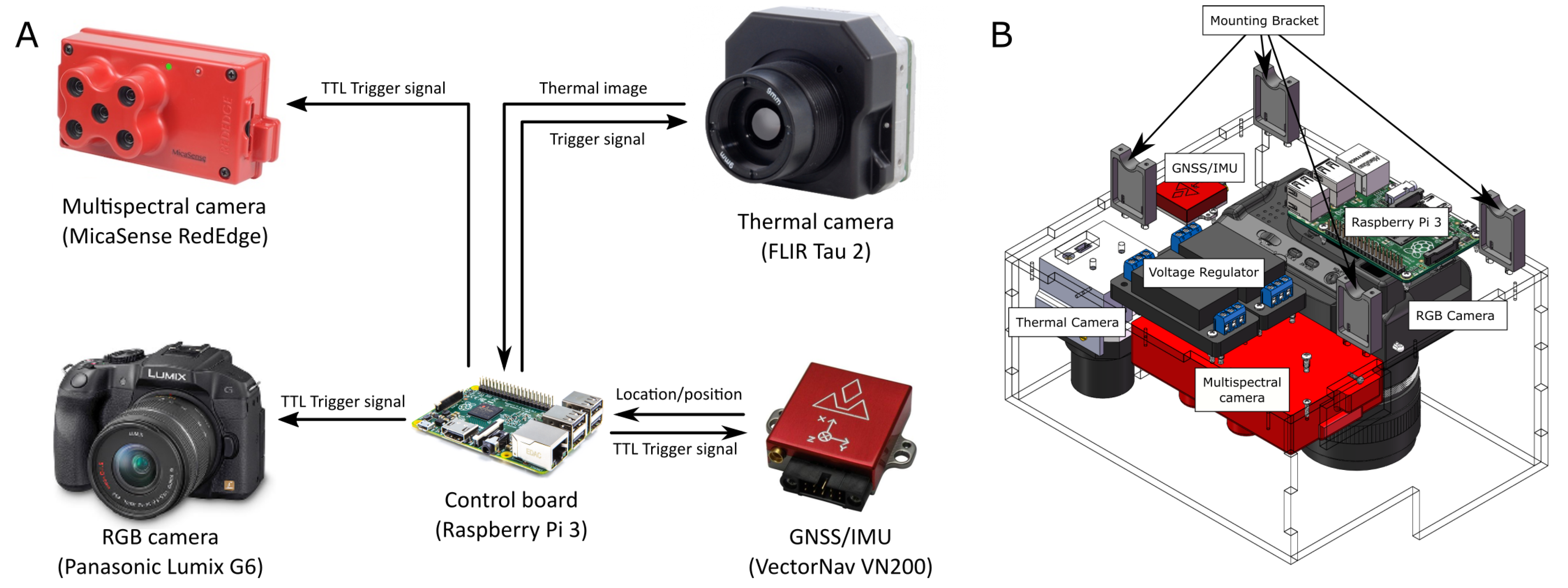
Figure 1. System diagram (A) and mechanical structure (B) of the first version of the data acquisition system.
Remotesensing 13 03517 g001
Figure 2. Mechanical structure of the DAS. The left figure is a rendered 3D model, and the right figure is the physical implemented system.
Remotesensing 13 03517 g002
Figure 3. RGB, multispectral and thermal cameras mounted on a low-payload UAV (Matrice 100, DJI, China). (A) Vertical mounting. (B) Horizontal mounting.
Remotesensing 13 03517 g003
Figure 4. Diagram of the electronic connection of the UAS.
Remotesensing 13 03517 g004
Figure 5. ROS computation graph. Ovals indicate nodes and rectangles indicate topics.
Remotesensing 13 03517 g005
Figure 6. Overall data processing pipeline.
Remotesensing 13 03517 g006
Figure 7. Thermal calibration targets. The customized device to record atmospheric conditions (highlighted by red rectangle) was mounted between the calibration targets.
Remotesensing 13 03517 g007
Figure 8. Testing field layout.
Remotesensing 13 03517 g008
Figure 9. GCPs in the field, including GCP for RGB and multispectral cameras (left) and GCP for thermal camera (right).
Remotesensing 13 03517 g009
Figure 10. Flight path recorded by the UAV during data collection. Distance between horizontal flight paths is 3.3   m . Direction of movement of thermal calibration targets is also indicated (left).
Remotesensing 13 03517 g010
Figure 11. Geometric distortion of the five bands of the multispectral camera. The orange cross indicates the image center. The red circle indicates the principal point. Contour lines indicate distortion in pixels. Arrows indicate the magnitude and direction of the distortion.
Remotesensing 13 03517 g011
Figure 12. Geometric distortion of the RGB and thermal camera. The orange cross indicates the image center. The red circle indicates the principal point. Contour lines indicate distortion in pixels. Arrows indicate the magnitude and direction of the distortion.
Remotesensing 13 03517 g012
Figure 13. Measured vignette, modeled vignette, and results of vignetting correction for each band of the multispectral camera.
Remotesensing 13 03517 g013
Figure 14. Vignetting effect of the thermal camera. The color bar indicates the temperature in degree Celsius.
Remotesensing 13 03517 g014
Figure 15. Atmospheric conditions recorded by the weather station on the ground during the flight. The transmittance of the atmosphere was estimated by using Equation (14).
Remotesensing 13 03517 g015
Figure 16. Correlation between image-derived temperatures ( T image ) and temperatures measured by the RTD ( T RTD ) for the thermal calibration targets.
Remotesensing 13 03517 g016
Figure 17. Overlay of UAV-derived orthomosaics, including RGB (background), temperature (section of mosaic; light yellow to black), and NDVI (section of mosaic; light green to dark green). Zoom-in images showing calibration targets, and the GCPs for the thermal camera are also displayed (bottom right).
Remotesensing 13 03517 g017
Figure 18. Illustration of a canopy segmentation result. The plot surface model was first subtracted by the ground plane to derive a plot height model. The canopy mask was generated by thresholding the RGB image and the height model for the plot.
Remotesensing 13 03517 g018
Figure 19. Correlation between maximum canopy height derived from images and maximum canopy height manually measured in the field.
Remotesensing 13 03517 g019
Figure 20. Visualization of the extracted phenotypical traits. The 99th percentile canopy height was used to represent the canopy height.
Remotesensing 13 03517 g020
Table 1. Specification of the sensors.
Thermal
Camera
Multispectral
Camera
DSLR
RGB Camera
Industrial
RGB Camera
LiDAR
ManufacturerFLIR systemsMicaSensePanasonicFLIR systemsVelodyne
ModelTau 2RedEdgeLumix G6GrassHopper3VLP-16
Dimensions (mm) 44.5 × 44.5 × 30 113 × 65 × 46 122 × 85 × 71 44 × 29 × 58 103 × 103 × 72
Weight (g)11215039090830
Resolution 640 × 512 1280 × 800 4608 × 3456 2448 × 2048 Vertical: 1.33 °
Horiz.: 0.1 ° –0.4 °
Focal length (mm)255.414–425N/A
Max FPS (Hz)30117520
Spectral range
( n m )
7500–13,500475, 560, 668,
717, 840
N/AN/AN/A
Accuracy (cm)N/AN/AN/AN/AUp to ±3
Table 2. Camera calibration parameters for the RGB, multispectral, and thermal cameras.
RGB
Camera
Multispectral CameraThermal
Camera
BlueGreenRedRedEdgeNIR
Focal length (mm)5.0045.4705.5135.4695.4775.49925.099
x p (mm)0.0720.0360.0410.0230.0280.049−0.049
y p (mm)0.0200.0610.000−0.045−0.0150.098−0.240
Skew angle (rad)8.26 × 10 4 −1.00 × 10 3 −1.87 × 10 3 −7.75 × 10 4 −1.14 × 10 3 −5.82 × 10 4 −3.12 × 10 3
K 1 −5.42 × 10 2 −9.78 × 10 3 −9.85 × 10 3 −2.61 × 10 2 −8.10 × 10 3 −1.09 × 10 2 −3.27 × 10 1
K 2 1.08 × 10 1 −1.57 × 10 1 −1.27 × 10 1 −5.42 × 10 2 −2.61 × 10 1 −7.20 × 10 2 1.77 × 10 0
K 3 −4.44 × 10 2 −4.38 × 10 1 −3.90 × 10 1 −4.66 × 10 1 1.71 × 10 1 −8.09 × 10 1 −3.61 × 10 1
P 1 −1.34 × 10 3 2.08 × 10 3 5.72 × 10 4 −1.55 × 10 3 −2.10 × 10 3 6.55 × 10 5 8.50 × 10 3
P 2 1.25 × 10 3 5.86 × 10 5 2.76 × 10 3 1.95 × 10 3 7.78 × 10 4 1.64 × 10 3 6.73 × 10 4
Table 3. Comparisons between canopy height derived from images and average canopy height manually measured in the field. H average : average canopy height. H median : median canopy height. H max : maximum canopy height. H np : n-th percentile canopy height MAE: mean absolute error. R 2 : coefficient of determination using linear model.
H average H median H max H 50 p H 60 p H 70 p H 80 p H 90 p H 99 p
MAE (m)0.5010.5310.1000.5310.4620.3950.3080.1960.060
R 2 0.7420.7990.6910.7990.6510.5430.4810.6190.766
Publisher’s Note: MDPI stays neutral with regard to jurisdictional claims in published maps and institutional affiliations.