Application of Multispectral Camera in Monitoring the Quality Parameters of Fresh Tea Leaves

Abstract

The production of high-quality tea by Camellia sinensis (L.) O. Ktze is the goal pursued by both producers and consumers. Rapid, nondestructive, and low-cost monitoring methods for monitoring tea quality could improve the tea quality and the economic benefits associated with tea. This research explored the possibility of monitoring tea leaf quality from multi-spectral images. Threshold segmentation and manual sampling methods were used to eliminate the image background, after which the spectral features were constructed. Based on this, the texture features of the multi-spectral images of the tea canopy were extracted. Three machine learning methods, partial least squares regression, support vector machine regression, and random forest regression (RFR), were used to construct and train multiple monitoring models. Further, the four key quality parameters of tea polyphenols, total sugars, free amino acids, and caffeine content were estimated using these models. Finally, the effects of automatic and manual image background removal methods, different regression methods, and texture features on the model accuracies were compared. The results showed that the spectral characteristics of the canopy of fresh tea leaves were significantly correlated with the tea quality parameters (r ≥ 0.462). Among the sampling methods, the EXG_Ostu sampling method was best for prediction, whereas, among the models, RFR was the best fitted modeling algorithm for three of four quality parameters. The R² and root-mean-square error values of the built model were 0.85 and 0.16, respectively. In addition, the texture features extracted from the canopy image improved the prediction accuracy of most models. This research confirms the modeling application of a combination of multi-spectral images and chemometrics, as a low-cost, fast, reliable, and nondestructive quality control method, which can effectively monitor the quality of fresh tea leaves. This provides a scientific reference for the research and development of portable tea quality monitoring equipment that has general applicability in the future.

1. Introduction

The Latin name of tea is Camellia sinensis (L.) O. Ktze, which is a popular beverage all over the world [1,2]. It is also an important cash crop in Qingyuan City, Guangdong Province, China, and dominates local agriculture as a characteristic industry [3,4]. Tea polyphenols, caffeine, free amino acids, total sugars, and other tea components have anti-oxidative, anti-cancerous, and anti-obesity characteristics, lower blood pressure, and prevent cardiovascular diseases [5,6,7,8,9,10]. In addition, the content of these components determines the qualities of taste, aroma, and appearance of tea [11], which, in turn, determine the tea quality and value [12]. Therefore, estimating and monitoring tea polyphenols and other quality parameters is significant in improving the tea quality and economic benefits associated with tea.

Traditionally, tea quality was evaluated by a professional tea taster, who judged the tea quality based on their sensory receptions. However, this method is inaccurate because of its subjective nature [13,14]; additionally, it can only be conducted after fresh tea leaves are converted into the final tea product, which is a time-consuming process. Conversely, tea quality can be more accurately evaluated by experimentally measuring the content of the main active components [15] using chemical composition analysis methods, such as gas chromatography mass spectrometry (GC-MS) [16]. However, such methods are inefficient, time-consuming, and destructive, and require technical expertise for their operation; additionally, their costs increase proportionally with the number of measurements [15]. Since 2019, the COVID-19 pandemic has severely impacted agriculture, especially with regard to labor and health and safety, but digital agricultural technology can provide alternative options to reduce personnel contact and labor restrictions during this period [17]. The development of sensors and nondestructive measurement technology in recent years has encouraged many scholars to study the application of new technologies, such as fluorescent nanotechnology [18], artificial olfaction based on colorimetric measurement [19], and the use of hyperspectrometers [20,21,22], to measure tea quality. These methods have been proven to deliver more accurate quality evaluation results compared to traditional methods, However, certain issues are associated with these methods. Nanotechnology uses toxic chemical reaction reagents, artificial olfaction technology is not mature enough [23], and hyperspectrometers are expensive and data acquisition and processing are time-consuming due to the large amount of data [24]. These issues limit their widescale application as a cheap, efficient, and nondestructive tea quality monitoring technology, and equipment is required.

This study investigated the use of an imaging multispectrometer for monitoring tea quality. Compared with the hyperspectrometer, it has low costs, fast data acquisition speed, and simple processing methods [25]. It is an improvement of hyperspectral technology [26]. In addition, imaging multi-spectral data includes both spectrum information and image information. Different tea genotypes and their expressions can cause differences in texture features of canopy images. Thus, to avoid this, the spectral and texture features were simultaneously extracted from the tea canopy images, and used to monitor the tea quality parameters. This has rarely been conducted in previous similar studies. Therefore, the present study presents novel methods to promote the widescale application of rapid tea quality assessment using stable and reliable machine learning methods to obtain a more universally acceptable tea quality parameter monitoring model.

2. Materials and Methods

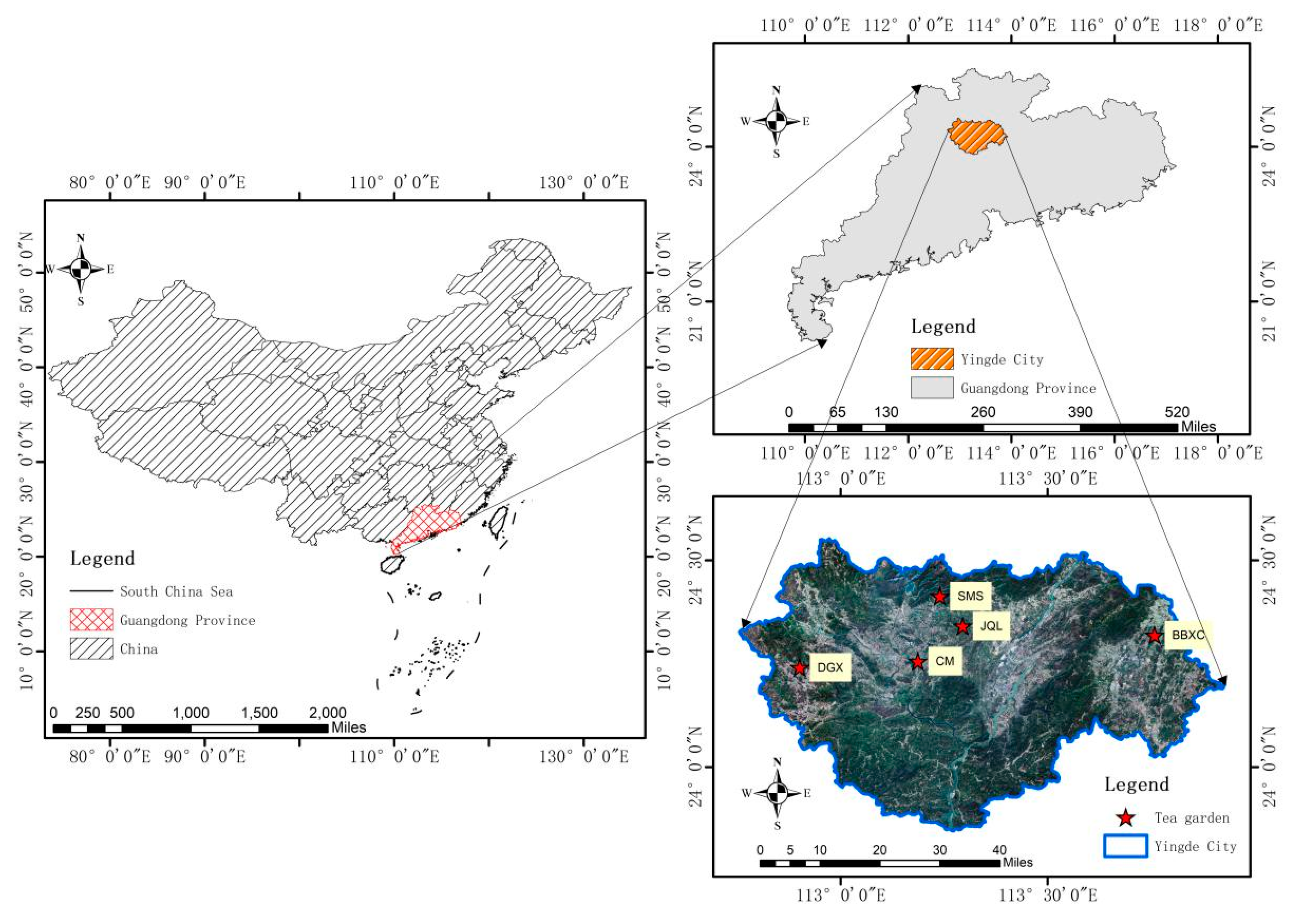
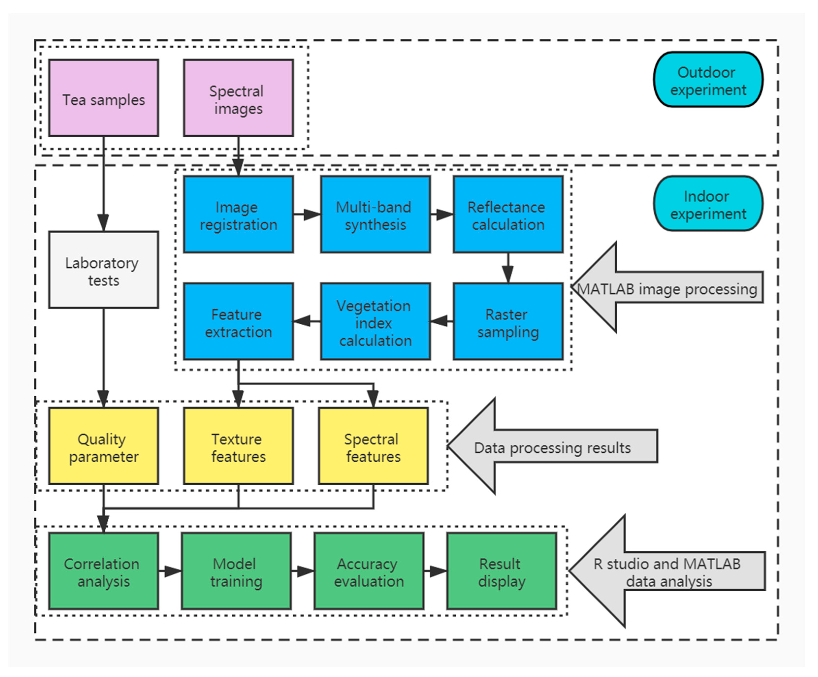
2.1. Experimental Program

The study area included five cooperative tea gardens Degaoxin, 800xiucai, Chuangmei, Jiqingli, and Shimenshan, in Yingde City, Qingyuan, Guangdong Province, China. Yingde City (23°50′31″–24°33′11″N, 112°45′15″–113°55′38″E) has a land area of 5634 km² [27] and is located in the transitional area from the south subtropical to the mid-subtropical zone. It has a subtropical monsoon climate, with long summers and short winters, sufficient sunshine, abundant rainfall, and an annual average temperature of 20.9 °C [28]. The geographical location of the study area is shown in Figure 1.

The experiment was conducted three times in May, July, and September 2020. The average temperature of the three experiments was 31, 35, and 30 °C, respectively. The experiment was conducted at noon on a clear and cloudless day. In each tea garden, more than 10 sampling points were randomly selected for spectral data and tea fresh leaf samples. Each sampling point was more than 10 m away from the edge of the road and the mutual distance was more than 100 m. The spectral image was taken through the vertical ground down and 1 m away from the canopy. The canopy spectral image including the calibration plate was taken three times for each sample point. At the same time, more than 250 g of one bud and two leaf samples were collected at the sample point for laboratory testing. The collected samples and spectral data included more than a dozen different tea varieties, mainly Yinghong No. 9, Huangdan, and Hongyan No. 12.

For the acquired spectral images, multi-band image registration, synthesis, reflectivity calculation, raster sampling, vegetation index calculation, and texture features extraction operations were performed in sequence. Correlation analysis and model training were performed on the obtained texture features and spectral features with laboratory test data, and, finally, the accuracy of the model was evaluated. The abovementioned data processing was implemented using MATLAB 2016b software, and the results were displayed using R studio software. The experimental steps are shown in Figure 2.

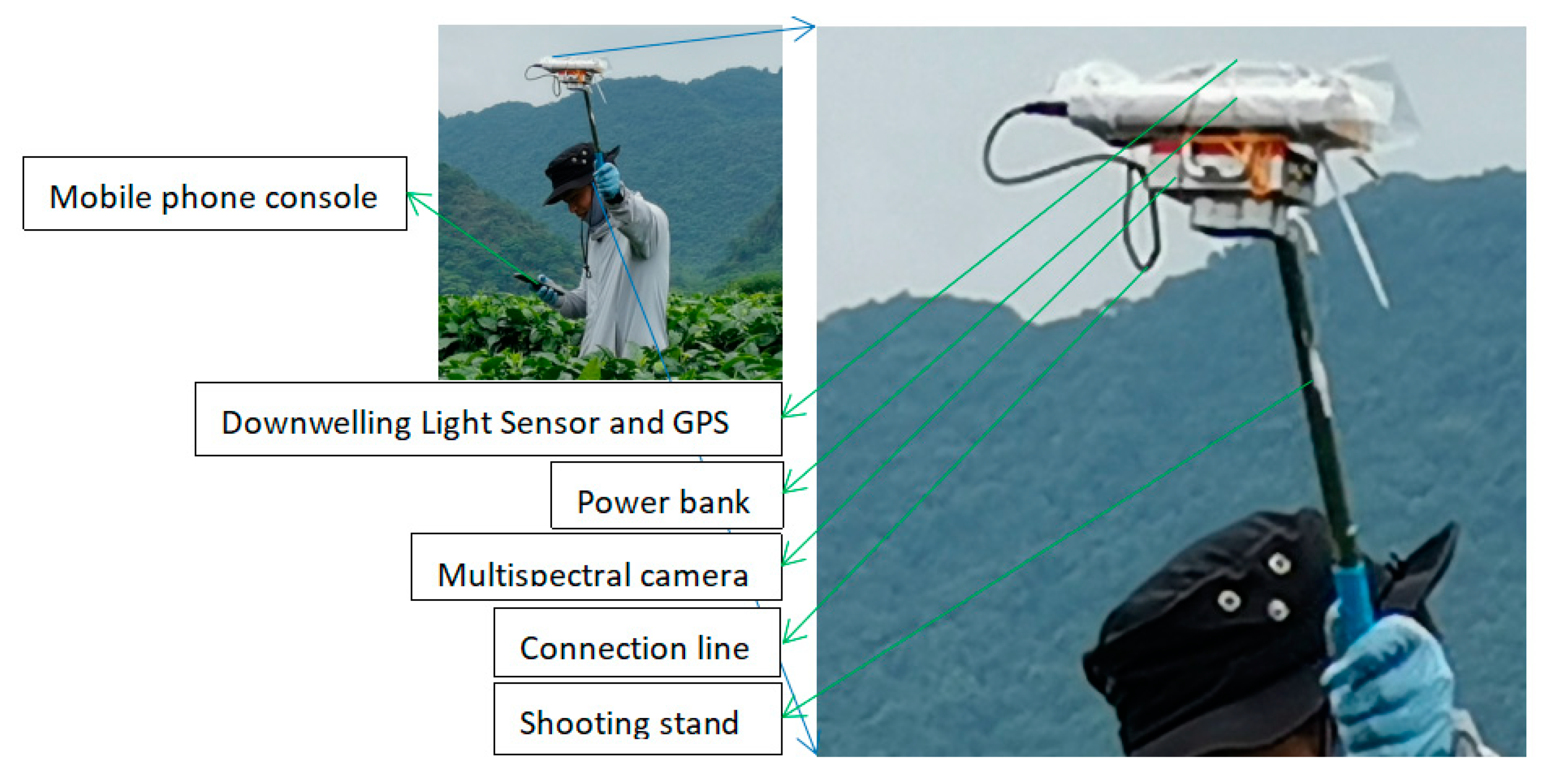
2.2. Data Acquisition

2.2.1. Spectral Data

The ground multispectral data used in this study were collected by a multispectral camera (RedEdge-MX, Micasense, Seattle, WA, USA), which has been widely used in the field of agricultural remote sensing [29]. The spectral parameters of the multispectral sensor are shown in

Table 1. Spectral parameters of multispectral sensor.

Band Number	Band Name	Center Wavelength (nm)	Bandwidth FWHM (nm)
1	Blue	475	20
2	Green	560	20
3	Red	668	10
4	Near-IR	840	40
5	Red Edge	717	10

FWHM = full-width-at-half-maximum

. The data acquisition system is shown in Figure 3.

Tea canopy images were acquired through the multi-spectral camera by shooting at a height of 80 cm from the tea tree canopies, and downward, perpendicular to the ground. A standard white board was placed at the center of the camera’s field of view and an attempt was made to ensure that the field of view completely included tea plants.

2.2.2. Quality Parameters

More than 250 g of fresh tea samples, with one bud and two leaves, were collected from the sampling points. The collected tea samples were dried and submitted to a third-party testing agency (Xi’an Guolian Quality Testing Technology Co. Ltd., Xi’an, China). Subsequently, the contents of tea polyphenols, caffeine, total sugars, and free amino acids were estimated by calculating them as a percentage of dry weight.

2.3. Methods

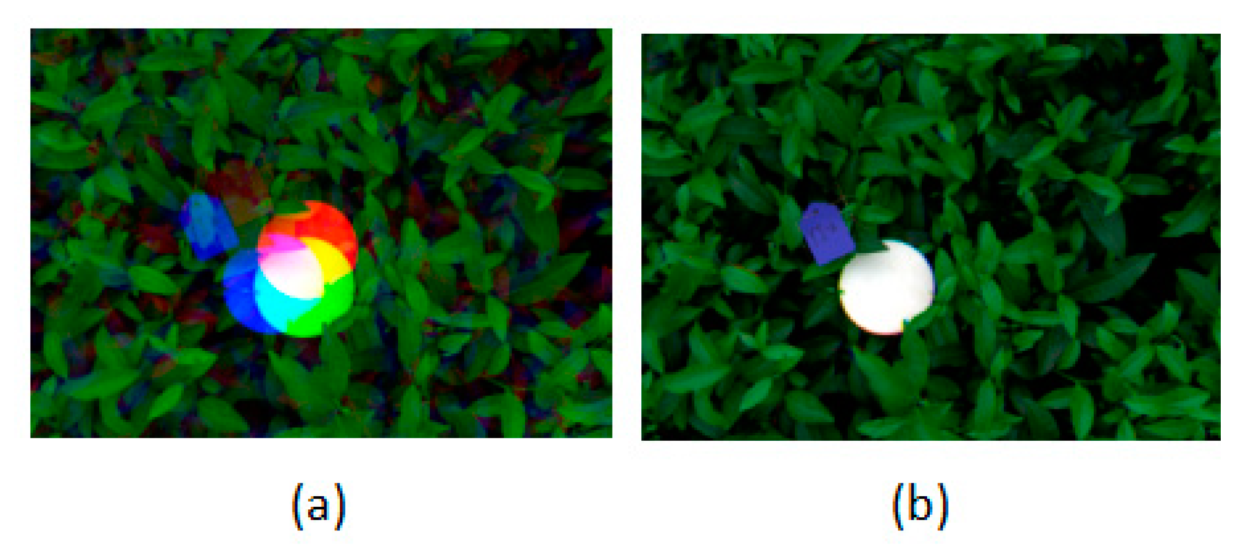
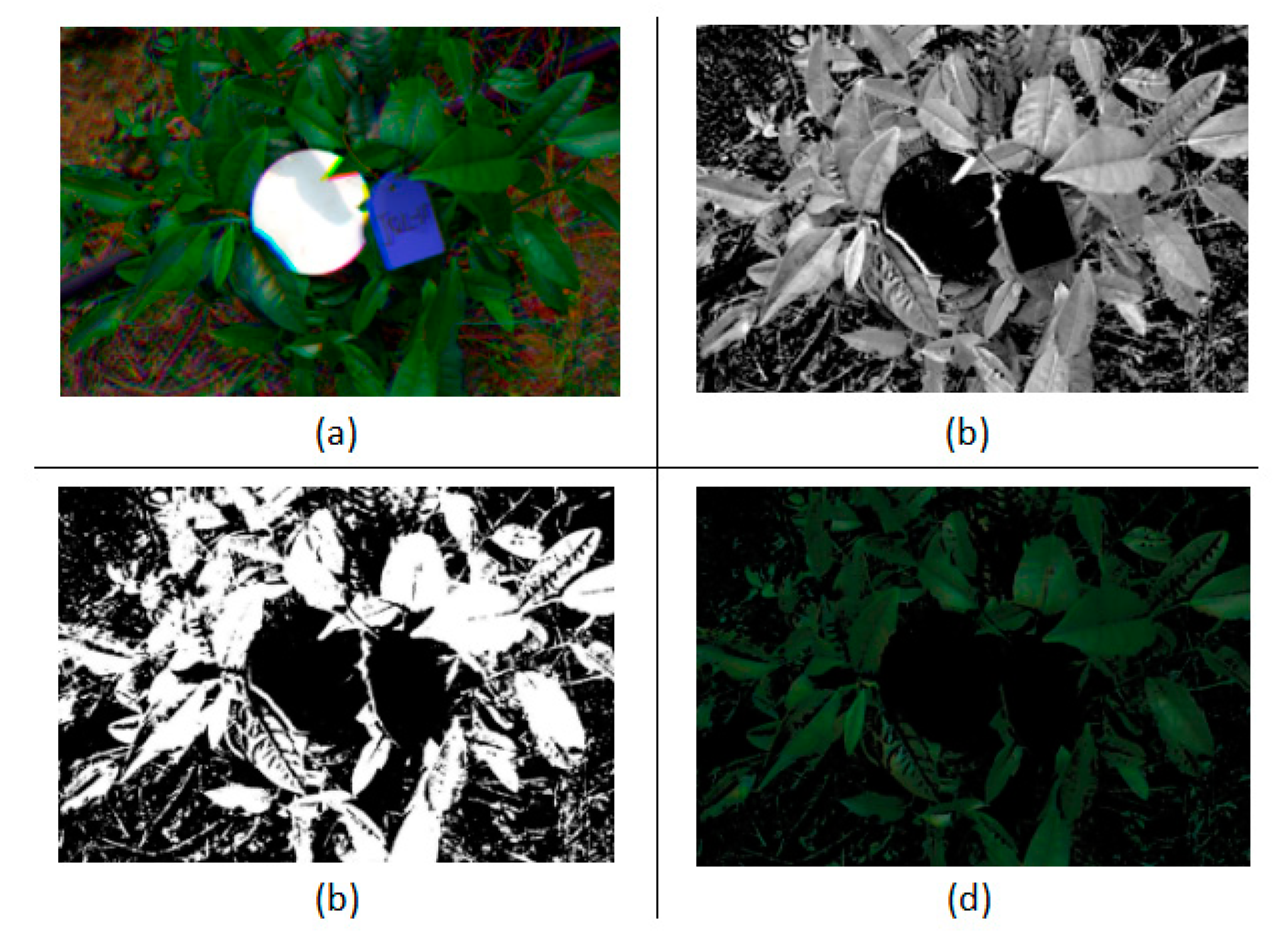
2.3.1. Image Processing

(1)

Registration program and band fusion

Tea canopy images were radiometrically calibrated with standard whiteboard digital numbers and digital number maps were converted to standard reflectance images to improve data quality. The sensor of each channel of the multispectral camera was distributed in an array, and the acquired images of each channel were spatially deviated; however, the cameras were not equipped with an automatic registration program. To facilitate band fusion and spectral information sampling, the Sift algorithm was used [30], and the features of each band image were automatically selected, matched, and finally, the bands were fused. An example of true color combination of the RGB three-channel combined image before and after registration is shown in Figure 4.

(2)

Raster sampling

To avoid the influence of soil and shadows in the captured images, the EXG [31] index was calculated in the combined image, and tea features were added in the image to distinguish tea from the background. Subsequently, the Ostu [32] method was used for image segmentation. After masking the background, pure tea areas in the image were finally obtained. The images corresponding to the above process steps are shown in Figure 5. Later, the average value of the area of the masked image was calculated. This group of average data is referred to as EXG_Ostu (EO) sampling data in the following sections. Additionally, the average value of the area of the image before removing the background was calculated. This dataset is referred to as Global (G) sampling data in the following section. Moreover, another dataset was added, 10 leaf positions on each image were manually added, and the average value was calculated. The data are referred to as Manual (M) sampling data in the following sections. The spectral data of the canopy tea leaves of the three sampling methods were extracted prior to further calculation and analysis.

2.3.2. Spectral Feature Construction

Previous studies have confirmed that the vegetation index can effectively improve the relationship between plant spectral information and physical and chemical parameters. Based on the actual situation, 24 commonly used vegetation indices were selected for calculation. The names and calculation formulas of the indices are shown in Table 2. In addition, 5 original single bands, 3 color components in hue saturation value color space, 4 discrete first-order derivatives, and a total of 36 parameters were used as spectral features. In order to distinguish the vegetation index G from the Green channel, this article refers to the Green channel as g.

Table 2. Vegetation indices compiled from the literature.

VIs	Formula	Reference	VIs	Formula	Reference
NDVI	NIR − R/NIR + R	[33]	RDVI	(NIR − ED)/SQRT(NIR + ED)	[34]
RVI	NIR/R	[35]	OSAVI	1.16(NIR − ED)/(NIR + ED + 0.16)	[36]
DVI	NIR − R	[37]	NLI	(NIR2 − ED)/(NIR2 + ED)	[38]
EVI	2.5(B − g)/(B + 6g − 7.5R + 1)	[39]	NDRE	(NIR − ED)/(NIR + ED)	[40]
VOG	(B − g)/(R + ED)	[41]	BGI	B/g	[42]
MTCI	(B − g)/(R − ED)	[43]	VARI	(R − g)/(g + R − B)	[44]
GNDVI	(NIR − g)/(NIR + g)	[45]	EXG	2g − R − B	[31]
WDRVI	(0.1NIR − R)/(0.1NIR + R)	[46]	BI	SQRT(R2 + g2)/2	[47]
GRVI	(g − R)/(g + R)	[48]	G	R/g	[42]
PSRI	(R − g)/ED	[49]	SIPI	(NIR − B)/(NIR + B)	[50]
RGR	R/g	[51]	MCARI	(B − g − 0.2(B − R))(B/g)	[52]
CCCI	(NIR − ED)/NIR + ED)/(NIR − R)/(NIR + R)	[53]	TGI	g + 0.39R − 0.61B	[54]

Notes: R, g, B, ED, and NIR are the reflectance in spectral bands of the red, green, blue, red-edge, and near-infrared, respectively. VI = vegetation index, NDVI = normalized difference vegetation index, RVI = ratio vegetation index, DVI = simple difference vegetation index, EVI = enhanced vegetation index, VOG = Vogelmenn red edge index, MTCI = MERIS terrestrial chlorophyll index, GNDVI = green normalized difference vegetation index, WDRVI = wide-dynamic-range vegetation index, GRVI = green-red vegetation index, PSRI = plant senescence reflectance index, RGR = red-green ratio index, CCCI = canopy chlorophyll content index, RDVI = renormalized difference vegetation index, OSAVI = optimized soil-adjusted vegetation index, NLI = nonlinear vegetation index, NDRE = normalized difference red edge, BGI = blue-green index, VARI = visible atmospheric resistance index, BI = brightness index, G = green, SIPI = structural independent pigment index, MCARI = modified chlorophyll absorption ratio index, and TGI = triangular greenness index.

Table 2. Vegetation indices compiled from the literature.

VIs	Formula	Reference	VIs	Formula	Reference
NDVI	NIR − R/NIR + R	[33]	RDVI	(NIR − ED)/SQRT(NIR + ED)	[34]
RVI	NIR/R	[35]	OSAVI	1.16(NIR − ED)/(NIR + ED + 0.16)	[36]
DVI	NIR − R	[37]	NLI	(NIR2 − ED)/(NIR2 + ED)	[38]
EVI	2.5(B − g)/(B + 6g − 7.5R + 1)	[39]	NDRE	(NIR − ED)/(NIR + ED)	[40]
VOG	(B − g)/(R + ED)	[41]	BGI	B/g	[42]
MTCI	(B − g)/(R − ED)	[43]	VARI	(R − g)/(g + R − B)	[44]
GNDVI	(NIR − g)/(NIR + g)	[45]	EXG	2g − R − B	[31]
WDRVI	(0.1NIR − R)/(0.1NIR + R)	[46]	BI	SQRT(R2 + g2)/2	[47]
GRVI	(g − R)/(g + R)	[48]	G	R/g	[42]
PSRI	(R − g)/ED	[49]	SIPI	(NIR − B)/(NIR + B)	[50]
RGR	R/g	[51]	MCARI	(B − g − 0.2(B − R))(B/g)	[52]
CCCI	(NIR − ED)/NIR + ED)/(NIR − R)/(NIR + R)	[53]	TGI	g + 0.39R − 0.61B	[54]

Notes: R, g, B, ED, and NIR are the reflectance in spectral bands of the red, green, blue, red-edge, and near-infrared, respectively. VI = vegetation index, NDVI = normalized difference vegetation index, RVI = ratio vegetation index, DVI = simple difference vegetation index, EVI = enhanced vegetation index, VOG = Vogelmenn red edge index, MTCI = MERIS terrestrial chlorophyll index, GNDVI = green normalized difference vegetation index, WDRVI = wide-dynamic-range vegetation index, GRVI = green-red vegetation index, PSRI = plant senescence reflectance index, RGR = red-green ratio index, CCCI = canopy chlorophyll content index, RDVI = renormalized difference vegetation index, OSAVI = optimized soil-adjusted vegetation index, NLI = nonlinear vegetation index, NDRE = normalized difference red edge, BGI = blue-green index, VARI = visible atmospheric resistance index, BI = brightness index, G = green, SIPI = structural independent pigment index, MCARI = modified chlorophyll absorption ratio index, and TGI = triangular greenness index.

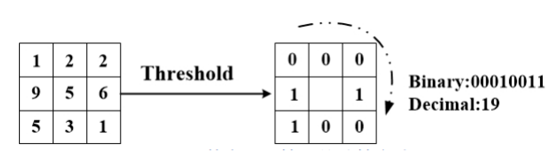
2.3.3. Texture Feature Extraction

In this study, gray level co-occurrence matrix (GLCM) [55,56,57,58] and local binary pattern (LBP) [59,60,61] methods were used to extract image texture features. The GLCM is a classic texture feature extraction method, which has been mostly used for auxiliary classification in previous research. Further, LBP has gained recent attention as a texture extraction method having a simple working principle and an excellent performance, and is mostly used for face recognition in artificial intelligence; Its basic coding principle is shown in Figure 6. The local differences in the tea canopy image are very subtle. As the EO and M sampling methods can destroy the image texture features, the standard whiteboard affects the texture features of the canopy image. In this study, 1/9th part of the upper right corner of the image was cropped to extract the LBP texture features; additionally, the GLCM extraction was set to 16 gray levels, a default direction, and a step size of 1. The principles of the two texture extraction methods are as follows:

LBP:

Figure 6. Basic LBP coding method.

Figure 6. Basic LBP coding method.

The calculation formula is:

$$LBP(x_c,y_c)={\displaystyle \sum _{p=0}^{p-1}{2}^p(S(i_p}-i_c)$$

(1)

$$S(x)=\{\begin{array}{l}1\hspace{1em}f\hspace{1em}x\ge 0\\ 0\hspace{1em}else\end{array}$$

(2)

where (x_c, y_c) are the coordinates of the central pixel, P is the P^th pixel in the field, i_c is the gray value of the pixel, i_p is the gray value of the central pixel, and S(x) is the sign function.

GLCM:

$$P(i,j|d,\theta )=\{(x,y)|f(x,y)=i,f(x+dx,y+dy)=j;\hspace{1em}x,y=0,1,2,\cdots ,N-1\}$$

(3)

where D is the relative distance expressed in pixels; θ is the texture calculation direction parameter, which is generally 0°, 45°, 90°, or 135°; i, j = 0, 1, 2, … L − 1; (x, y) are the pixel coordinates in the figure; and L is the gray level.

The statistics of grayscale images after GLCM and LBP re-encoding are generally used to describe features. In this study, energy (Asm), entropy (Ent), contrast (Con), correlation (Cor), and their respective variances were selected as the descriptors of the GLCM texture features. The average gray level (μ), mean square error (σ), skewness (S), kurtosis (K), energy (G), information entropy (E), and smoothness (R) of the histogram of the LBP-encoded image were selected as the descriptors of the LBP texture features. These descriptors were calculated as follows:

GLCM:

$$Asm={\displaystyle \sum }_{i=0}^{N-1}{\displaystyle \sum }_{j=0}^{N-1}{[P\left(i,j,d,\theta \right)]}^2.$$

(4)

$$Ent=-{\displaystyle \sum }_{i=0}^{N-1}{\displaystyle \sum }_{j=0}^{N-1}P\left(i,j,d,\theta \right){\log }_{2}P\left(i,j,d,\theta \right).$$

(5)

$$Con={\displaystyle \sum }_{i=0}^{N-1}{n}_2\{\hspace{0.17em}{{\displaystyle \sum }}_{\left|i-j\right|=n}P\left(i,j,d,\theta \right)\}.$$

(6)

$$Cor=\frac{{\displaystyle {\displaystyle \sum }_{i=0}^{N-1}}{\displaystyle {\displaystyle \sum }_{j=0}^{N-1}}\left(ijP\left(i,j\right)\right)-u_1{u}_2}{{\sigma }_1^2{\sigma }_2^2}.$$

(7)

among which

$$\begin{array}{l}{u}_1={\displaystyle \sum _{i=0}^{N-1}{\displaystyle \sum _{j=0}^{N-1}iP(i,j,d,\theta )}},\hspace{1em}\hspace{1em}\hspace{1em}\hspace{1em}{u}_2={\displaystyle \sum _{i=0}^{N-1}{\displaystyle \sum _{j=0}^{N-1}jP(i,j,d,\theta )}},\\ {\sigma }_1^2={\displaystyle \sum _{i=0}^{N-1}(i-u_1}{)}^2{\displaystyle \sum _{j=0}^{N-1}P(i,j,d,\theta )},\hspace{1em}\hspace{1em}\hspace{1em}\hspace{1em}{\sigma }_2^2={\displaystyle \sum _{i=0}^{N-1}(i-u_2}{)}^2{\displaystyle \sum _{j=0}^{N-1}P(i,j,d,\theta )}\end{array}$$

LBP:

$$\mu ={\displaystyle \sum }_{g=0}^{L-1}gP\left(g\right).$$

(8)

$$\sigma =\sqrt{{\displaystyle \sum }_{g=0}^{L-1}(g-\mu {)}^{2}P\left(g\right)}.$$

(9)

$$S={\displaystyle \sum }_{g=0}^{L-1}{(g-\mu )}^{3}P\left(g\right).$$

(10)

$$K=\frac{1}{{\sigma }^4}{\displaystyle \sum }_{g=0}^{L-1}{(g-\mu )}^{4}P\left(g\right).$$

(11)

$$G={\displaystyle \sum }_{g=0}^{L-1}P{(g)}^2.$$

(12)

$$E=-{\displaystyle \sum }_{g=0}^{L-1}P\left(g\right){\log }_2\left[P\left(g\right)\right].$$

(13)

$$R=\frac{1}{1+{\sigma }^2}.$$

(14)

where P(g) is the LBP coded image, μ is the average gray level of the image, σ is the mean square error reflecting the average image contrast, S is the skewness reflecting the symmetry of the histogram distribution, and K is the closeness of the image gray level to the mean value. The kurtosis of G is the energy reflecting the image uniformity, E is the information entropy reflecting the randomness of the image grayscale, and R is the smoothness reflecting the relative smoothness of the image.

2.3.4. Feature Selection

Correlation analysis is a conventional and effective dimensionality reduction method. We analyzed the correlation between spectral and texture features and tea quality parameters and selected 10 features with the highest absolute values of correlation coefficients for linear regression to reduce calculations.

2.3.5. Regression Modeling

Several simple and effective regression modeling algorithms, such as partial least squares regression (PLS), support vector machine regression (SVR), and random forest regression (RFR), were used in this study. Among these, PLS is widely used to study the relationship between multiple dependent and independent variables. It combines the advantages of principal component analysis, normative analysis, and linear regression, and can effectively acquire the dominant factor with the strongest explanatory power for the dependent variable. PLS is especially used to solve problems, such as multicollinearity between variables or when the number of variables is more than the sample number [62,63]. The linear relationship between spectral data and chemical composition can be successfully modeled, especially in the presence of multiple dimensions and multicollinearity in the original spectral data [64]. SVR can provide a more rational solution to the above-mentioned problems than the linear method can [65]. SVR uses a kernel function to map input variables to a high-dimensional feature space [66]; therefore, it can process high-dimensional input vectors. Recently, SVR has been widely used in spectral analysis, subsequently producing accurate calibration results [67,68,69,70]. The RFR algorithm is an integrated learning algorithm that combines a large number of regression trees, which represent a series of conditions or constraints that are organized in a hierarchical structure and applied sequentially from the root to the leaves of the tree. RFR starts with multiple guide samples, which are randomly drawn from the original training dataset. Subsequently, the regression tree is applied to each bootstrap sample. A small group of input variables selected from the total set are randomly considered for the binary partitioning of each tree node [71,72,73].

2.3.6. Accuracy Evaluation

The coefficient of determination (R²) and root-mean-square error (RMSE) were used to comprehensively evaluate the model accuracy. The verification method used random subsampling verification (hold-out method) and the two parameters were calculated as follows:

$${\mathrm{R}}^2=1-{\displaystyle {\sum }_{i=1}^n(x_i-y_i}{)}^2/{\displaystyle {\sum }_{i=1}^n(x_i}-\overline{x}{)}^2$$

(15)

$$\mathrm{RMSE}=\sqrt{{\displaystyle {\sum }_{i=1}^n(x_i}-y_i{)}^2/n}$$

(16)

where x_i is the real measured value, y_i is the predicted value, $\overline{x}$ is the average of the measured values, and n is the number of samples.

3. Results

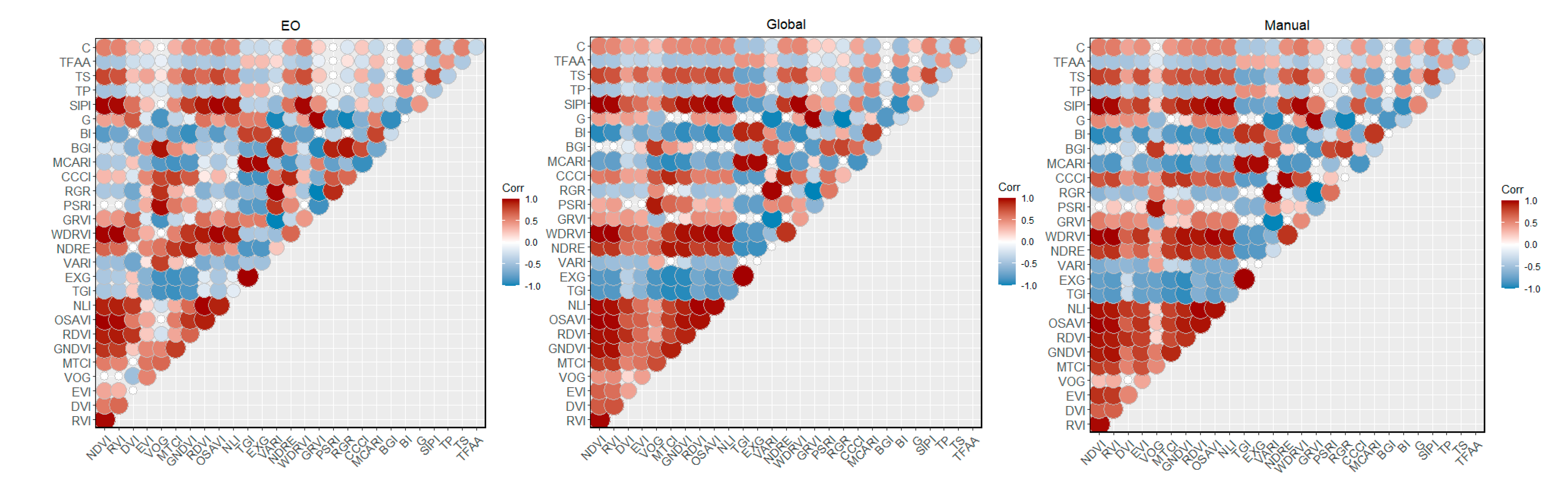
3.1. Correlation Analysis

The correlation between tea quality parameters and spectral indices is shown in Figure 7. The ten features having the highest correlation coefficients with the tea quality parameters are shown in

Table 3. Most relevant indices and their correlation coefficients.

Tea Polyphenols		Total Sugars		Free Amino Acids		Caffeine
VIs	Correlations	VIs	Correlations	VIs	Correlations	VIs	Correlations
NDVI	0.462	WDRVI	0.782	BI	0.475	G	0.546
OSAVI	0.462	SIPI	0.783	NDVI	0.483	GNDVI	0.551
WDRVI	0.464	ED	0.791	OSAVI	0.483	V	0.565
R	0.471	NDVI	0.796	RVI	0.491	R	0.567
BI	0.499	OSAVI	0.796	WDRVI	0.491	B	0.571
V	0.523	B	0.8030	NDRE	0.5	SIPI	0.592
NDRE	0.534	BI	0.812	V	0.503	NDVI	0.593
G	0.543	R	0.8150	G	0.516	OSAVI	0.593
GNDVI	0.544	G	0.8150	GNDVI	0.52	RVI	0.596
ED	0.556	V	0.8270	ED	0.522	WDRVI	0.598

.

It can be seen from Figure 5 that there are significant differences in the correlation analysis results between the spectral parameters and the quality parameters under the three sampling methods, but most of the correlations have reached a significant level, which indicates that the quality parameters of tea are clearly related to the spectral parameters. The spectral response mechanism is consistent, which is the basis for steps in this study. In addition, this also means that different spectral data grid sampling methods will affect the strength of this connection and need to be considered.

Generally, the red (R), red-edge (ED), and near-infrared (NIR) bands are particularly sensitive to the physical and chemical properties of plants. In this study, most spectral features were significantly correlated with the quality parameters, and among the most relevant indexes, almost all were related to R, ED, and NIR band data, which were used to calculate and construct these indexes. This is consistent with previous research results, which observed a strong correlation between the crop physical and chemical parameters with the spectral characteristics.

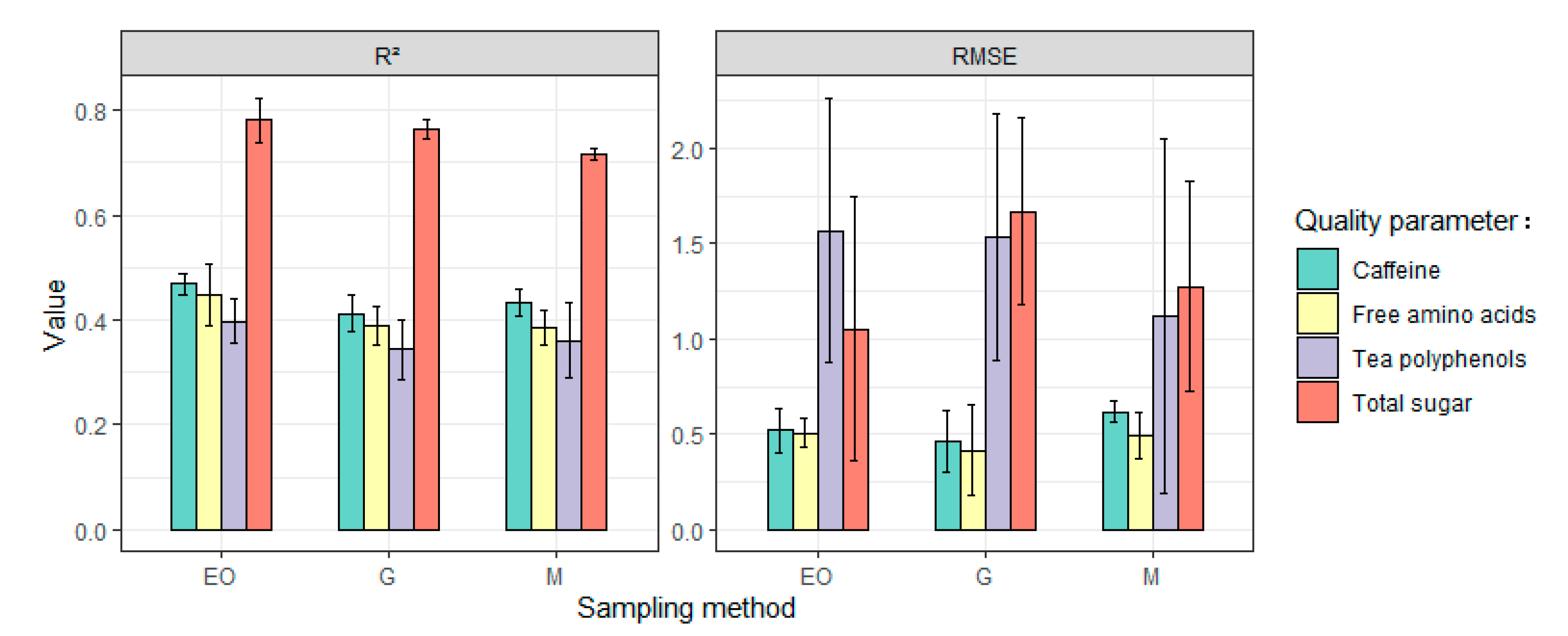
3.2. Best Fit Sampling Method

The spectral feature parameters and quality parameters obtained by the EO, G, and M sampling methods were trained to build models through the PLS, SVR, and RFR algorithms, respectively. The final average prediction results of the three models for each sampling method are shown in Figure 8, which indicates that the R² values of the quality parameters of the EO sampling method and the spectral characteristic model are highest, and the overall RMSE is relatively low. This indicated that the EO sampling method used in this study can effectively reduce the impact of soil and other background noise, improve the data authenticity, and has an evidently positive effect on model prediction accuracy.

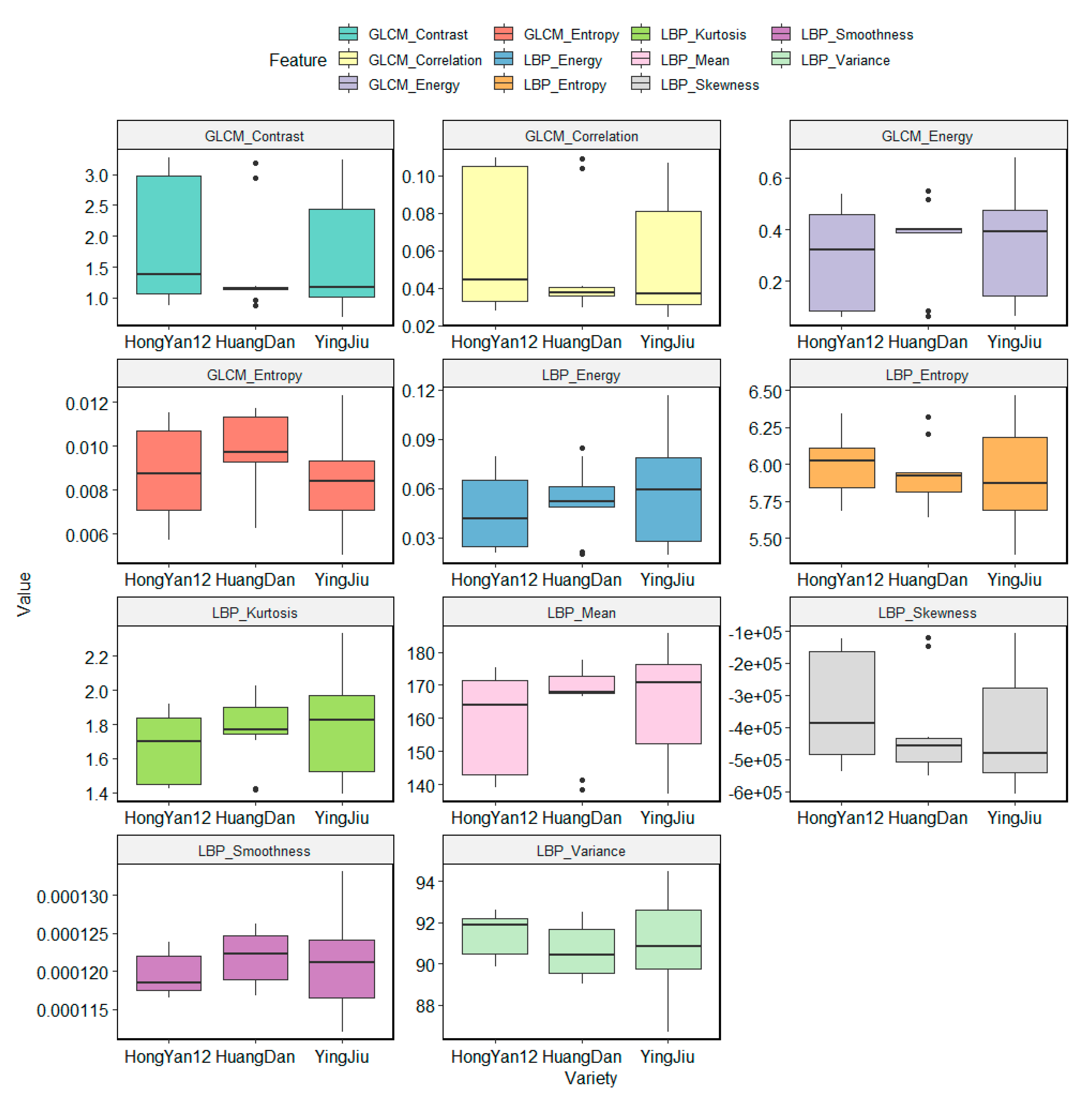
3.3. Tea Varieties and Canopy Texture Features

Tea samples of more than 10 varieties were used in this study. Among these, Yinghong No. 9, Huangdan, and Hongyan No. 12 were the main varieties. The texture features of these three varieties were extracted using the texture information extraction method. The consequent results are shown in Figure 9. The descriptive statistics of texture information extracted by different varieties were evidently different. Particularly, the LBP texture features were more different than those of GLCM. This shows that texture features can help distinguish tea varieties, thereby promoting tea quality monitoring.

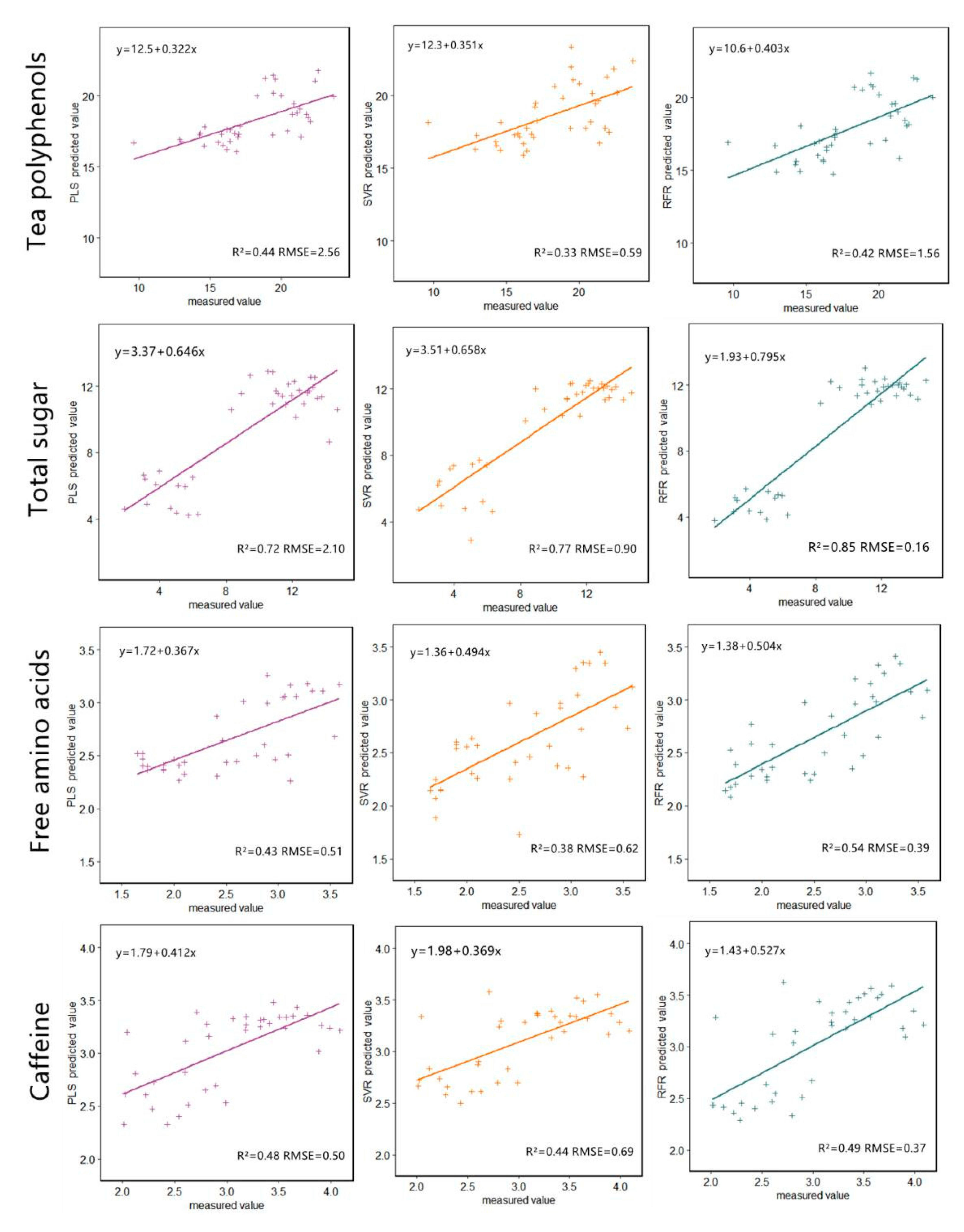
3.4. Best Fit Modeling Algorithm

The EO method was used for sampling, and the predicted values of the tea quality parameters calculated using the three models trained by the PLS, SVR, and RFR algorithms were compared with the measured values. The results are shown in Figure 10. Different best-fit model training methods were observed for predicting the results of various tea quality parameters. The PLS and SVR algorithms were the best fits for tea polyphenol prediction and least error, respectively. RFR was the best fit for the total sugar prediction model and had the smallest error. RFR was also the best fit for the free amino acid prediction model and had the smallest error. Additionally, RFR was the best fit for the caffeine prediction model and had the smallest error. Thus, RFR was the best fitted modeling algorithm for three of the four quality parameters. Based on the comprehensive goodness of fit and error factors of tea polyphenols, the best fitted modeling algorithm was RFR.

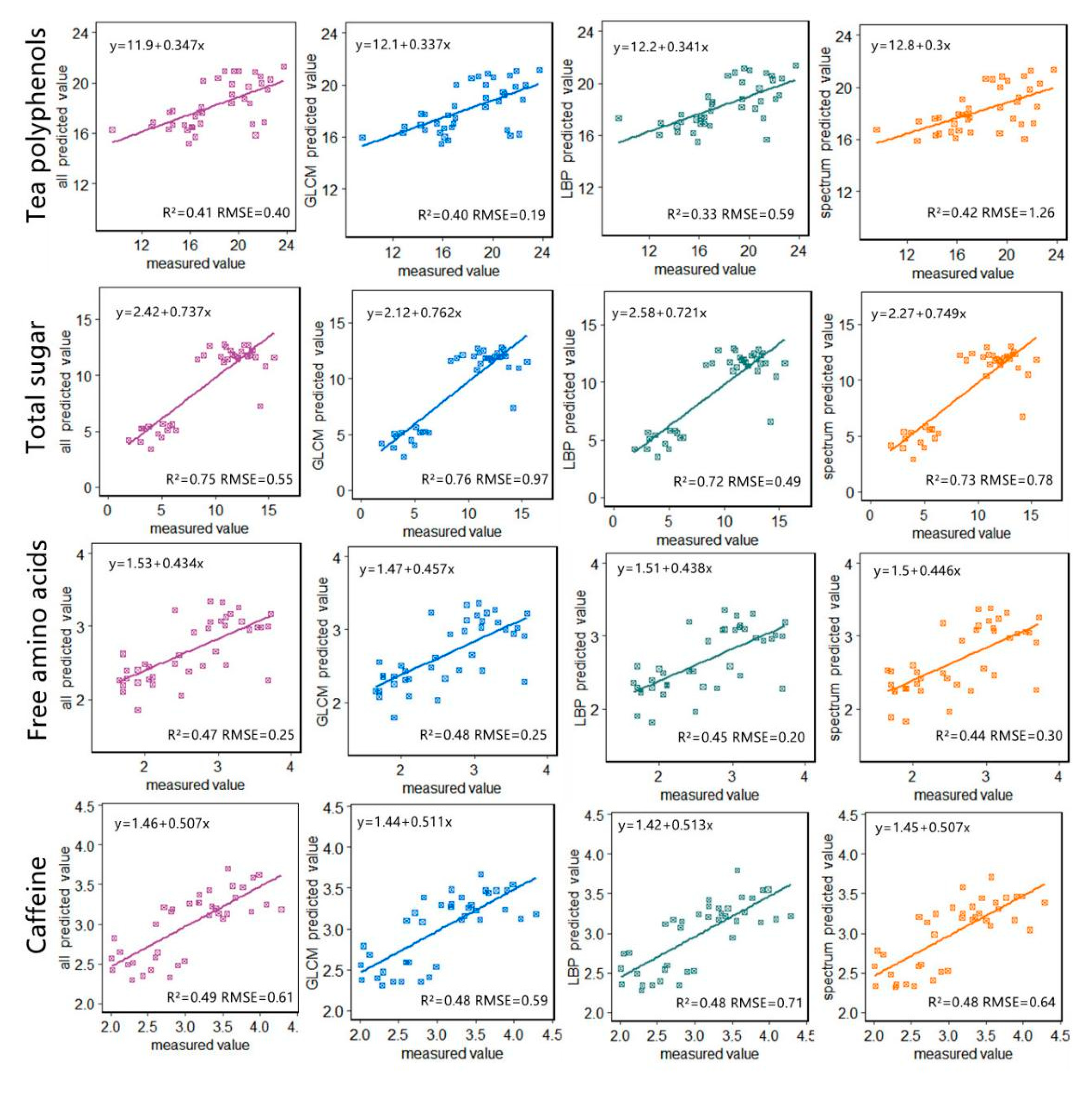
3.5. Effect of Texture Features on Model Accuracy

The EO and M sampling methods can destroy the texture information of the original image; additionally, a standard whiteboard in the center of the image should be eliminated; therefore, we used the G sampling method and selected the 1/9 image scale in the upper right corner of the original image. While using this method, background objects, such as soil, should be absent in the selected image. The modeling method selected the best RFR, the accuracies of which before and after adding the texture features are shown in Figure 11. After the integration of the tea polyphenol prediction model with texture features of LBP and GLCM, the result errors reduced, but the goodness of fit of the model did not improve. Conversely, after the prediction model of total sugar was integrated with GLCM texture features, the goodness of fit improved and the result errors increased. The LBP texture features did not improve the model goodness of fit and reduced the prediction result errors, whereas the goodness of fit and the prediction result errors of the model integrated with texture features of both GLCM and LBP improved. The prediction model of free amino acids integrated with texture features improved the goodness of fit and the accuracy of prediction results. The goodness of fit of the caffeine prediction model did not significantly improve after the integration of texture features, but GLCM texture features reduced the prediction result errors. Overall, the tea quality parameter monitoring model that integrated texture features showed higher prediction accuracy, with GLCM contributing more to improving the model accuracy than LBP.

4. Discussion

4.1. Ground Multispectral Images

RedEdge is a 5-discrete-narrowband frame multispectral sensor that is commonly used in remote-sensing studies and precision agriculture [74,75,76,77,78]. It is considered stable and reliable, and as an improved product of hyperspectral technology, its costs have reduced drastically [25,26], thus broadening its applicability in tea quality monitoring. Previous studies have typically integrated RedEdge-mx in unmanned aerial vehicles [74,75,77,78], which means more complex data acquisition steps, lower spatial resolution, and more data processing procedures. Close-range applications are limited [76]; however, the ground portable handheld method proposed in this study can obtain reliable multi-spectral data more easily and accurately compared to application with unmanned aerial vehicles.

However, a small proportion of ground objects that are not classified as tea in the ground multispectral images can affect the final quality of the parameter monitoring results. In order to reduce the influence of soil and shadow noise and improve the accuracy of the final quality parameter monitoring results, this study used the EXG index to effectively distinguish the background of green vegetation and soil for image enhancement [31,79,80,81,82]. The Ostu method was used for image segmentation [32,83,84,85,86] to enable the effective extraction of the tea areas from the original image that contains other features. In comparison, the predicted results of the model using the EO sampling method were more accurate than the models using the G and M sampling methods. This was because background factors, such as soil, act as noise and interfere considerably with the sampling results of the G method; furthermore, the M sampling method completely depends on human subjective judgment and loses the objective representativeness of the sample. Conversely, the EO sampling method ensures objectivity while reducing the impact of noise. Notably, in this study, noise elimination is only applicable to green tea varieties. For tea images of other color varieties, the noise and the tea area will still be mixed. Finding a vegetation index that can enhance the characteristics of these nongreen tea varieties should help eliminate noise.

4.2. Vegetation Characteristics

Relative to the original spectral information, the vegetation index constructed by fusing multispectral bands can highlight specific vegetation characteristics, and is widely used to monitor plant physiological and biochemical parameters, such as biomass, total nitrogen content, and chlorophyll content [87,88,89]. Additionally, some vegetation indices can suppress the influence of soil noise [90,91]. Therefore, in this study, the vegetation index was calculated to enhance the relationship between the spectral characteristics and quality parameters, and eliminate the influence of soil and shadow noise. Correlation analysis results show that the vegetation indices with the strongest correlations with tea polyphenols, total sugars, amino acids, and caffeine were GNDVI (r = 0.544), BI (r = 0.812), GNDVI (r = 0.52), and WDRVI (r = 0.598), thus confirming the necessity of vegetation index calculation. In addition, the vegetation index showed the highest correlation (r ≥ 0.462) with tea quality parameters and was correlated with R, ED, and NIR. In fact, ED has been most widely used as a spectral feature for evaluating crop parameters [45,92,93,94,95,96,97], and NIR is also a key component of most vegetation indices [98,99]. This indicates that the correlation analysis results in this study are consistent with those of previous studies. However, the vegetation index calculated in this study has certain limitations. The development of a method that more strongly correlates vegetation with tea quality parameters can improve the accuracy of tea quality monitoring results.

Spectral images have wide applications and integration with maps. It not only provides the spectral information of the target, but also obtains the spatial information [100,101,102]. In remote sensing image classification, the spatial location, shape, and texture characteristics of ground objects are particularly important [103,104,105]. In previous studies, some scholars have used remote sensing image texture information for machine classification, and have achieved good results [55,59,106,107,108], but few studies have been conducted using the texture information for regression. Samples of different tea varieties were used in this study. Based on the relationship between genotype and expressiveness, the difference in texture features can help distinguish different varieties, thereby improving the estimation accuracy of quality parameters. Therefore, in this study, the texture features of GLCM and LBP were extracted from the multispectral image. As a classic texture feature extraction method, GLCM is widely used in machine vision, and its performance has been recognized by scholars [109,110,111,112,113]. In this study, 16-level grayscale and a step size of 1 were set when extracting GLCM texture features. Although the number of calculations is large, it can improve the detailed texture. The default direction was set because the distribution direction of the leaf canopy of tea leaves is random, and the difference caused by the direction parameter settings of different sliding windows is very small. In this study, the LBP texture feature extraction method, which was developed for better facial recognition, and has gradually been applied in facial recognition [114,115] and agriculture [116], was applied. In this study, the texture features of GLCM and LBP were combined with spectral features to estimate tea quality parameters. The subsequent results confirmed that the texture information can improve the accuracy of estimating the tea quality parameters, but its effect was not significant. This could be attributed to many reasons. First, to preserve the original image texture information, the upper right corner of the original image was used to extract the texture features, thus promoting the influence of noise, such as soil and shadows, in some images on the texture feature. Second, the 15 texture features selected in this study included GLCM and LBP, but the texture features that were actually closely related to the tea quality parameters were excluded. Finally, texture features and spectral features were input to the model for training simultaneously with dependent variables, and other feature integration methods, such as constructing hierarchical models, were not applied.

4.3. Modeling Methods

The PLS, SVR, and RFR algorithms are regression modeling methods that have been proven to be concise, stable, and effective in recent studies [67,68,69,70]. Among them, PLS is considered the simplest and does not require many parameters in the training process. Moreover, inputting variables can eliminate the multicollinearity in the x independent variables and reduce the data dimension. The obtained descriptive variables are the best choice for predicting the dependent variable y [117,118,119,120]. For fair comparison, in this study, the radial basis function kernel and other default parameters were set in the SVR model training, and 500 decision trees and other default parameters were set in the RFR model training. The PLS, SVR, and RFR algorithms took 6.063, 23.617, and 3.032 s to train with the same data in MATLAB, respectively. In this study, the RFR was the best model algorithm and had the highest operating efficiency. These characteristics facilitate the development and promotion of subsequent corresponding technologies and equipment. The analysis results did not indicate a considerable difference in the goodness of fit of the three models of tea polyphenols, total sugars, free amino acids, and caffeine. The R² of all the quality parameter monitoring models were between 0.33 and 0.85. The SVR model of tea polyphenols using the EO sampling method had R² > 0.4, whereas the RF model incorporated the texture features of LBP. According to the characteristics of SVR [121], the reason for the former is that the SVR model of tea polyphenols is under-fitting, whereas the latter is because when the monitoring model fuses with LBP texture features, soil and shadow noise interfere; thus, the application of LBP texture features yields negligible improvement in the accuracy of tea polyphenols monitoring. Generally speaking, the R² value achieved is similar to results in previous research [122]. In this study, the RMSE differed considerably between the models, with a higher RMSE for PLS than the other two methods. This was because the PLS is a linear regression, and most data in practical situations do not show a simple linear relationship [65]. Therefore, the error of the prediction results of the linear models is higher than that of the nonlinear machine learning models.

5. Conclusions

This study investigated the application of low-cost, high-efficiency, high-precision, and easily applicable tea quality monitoring methods. R, ED, and NIR were the sensitive bands of tea quality parameters and are also sensitive to most other plants. The EO sampling method based on feature enhancement of the EXG index and the binary segmentation of the Ostu method assisted in acquiring more accurate and representative spectral sampling results. Compared with the G and M sampling methods, the EO method avoids soil, shadow, and human subjectivity. The influence of the above-mentioned factors facilitated the improvement of the prediction accuracy of the tea quality monitoring model. Furthermore, the GLCM and LBP texture features of the tea canopy image showed differences in the different tea varieties. To a certain extent, they improved the prediction accuracy of the of tea quality monitoring model, with the GLCM texture features contributing to a higher model accuracy than the LPB does. Among the four tea quality parameters of tea polyphenols, total sugars, free amino acids, and caffeine, the monitoring effect of total sugar was best (R² = 0.85 and RMSE = 0.16). Among the three modeling methods (PLS, SVR, and RFR), the RFR method showed the highest prediction accuracy. The proposed method can assist in developing universally acceptable portable tea quality monitoring equipment suitable for monitoring multiple tea varieties and can improve the tea monitoring efficiency and accuracy.

References

1. Yang, C.S.; Wang, Z.Y. Tea and cancer. J. Natl. Cancer Inst. 1993, 85, 1038–1049. [Google Scholar] [CrossRef]
2. Yang, C.S.; Lambert, J.D.; Sang, S. Antioxidative and anti-carcinogenic activities of tea polyphenols. Arch. Toxicol. 2009, 83, 11–21. [Google Scholar] [CrossRef] [PubMed] [Green Version]
3. Xu, J. Discussion on qingyuan tea industry development strategy based on SWOT analysis. Guangdong Tea Ind. 2016, 3, 5–8. [Google Scholar]
4. Gao, H.; Zhang, M. Analysis of the status quo and countermeasures of the tea industry development in Yingde City. Guangdong Tea Ind. 2019, 5, 25–29. [Google Scholar]
5. Jiang, H.; Xu, W.; Chen, Q. Evaluating aroma quality of black tea by an olfactory visualization system: Selection of feature sensor using particle swarm optimization. Food Res. Int. 2019, 126, 108605–108611. [Google Scholar] [CrossRef] [PubMed]
6. Zhang, L.; Santos, J.S.; Cruz, T.M.; Marques, M.B.; Carmo, M.A.V.; Azevedo, L.; Granato, D. Multivariate effects of Chinese keemun black tea grades (Camellia sinensis var. sinensis) on the phenolic composition, antioxidant, antihemolytic and cytotoxic/cytopro-tection activities. Food Res. Int. 2019, 125, 108516–108525. [Google Scholar] [CrossRef] [PubMed]
7. Zhou, P.; Zhao, F.; Chen, M.; Ye, N.; Lin, Q.; Ouyang, L.; Wang, Y. Determination of 21 free amino acids in 5 types of tea by ultra-high performance liquid chromatography coupled with tandem mass spectrometry (UHPLC–MS/MS) using a modified 6-aminoqui- nolyl-N-hydroxysuccinimidyl carbamate (AQC) method. J. Food Compos. Anal. 2019, 81, 46–54. [Google Scholar] [CrossRef]
8. Mukhtar, H.; Ahmad, N. Tea polyphenols: Prevention of cancer and optimizing health. Am. J. Clin. Nutr. 2000, 71, 1698–1702. [Google Scholar] [CrossRef] [Green Version]
9. Westerterp-Plantenga, M.S.; Lejeune, M.P.G.M.; Kovacs, E.M.R. Body weight loss and weight maintenance in relation to habitual caffeine intake and green tea supplementation. Obes. Res. 2005, 13, 1195–1204. [Google Scholar] [CrossRef]
10. Miller, P.E.; Zhao, D.; Frazier-Wood, A.C.; Michos, E.D.; Averill, M.; Sandfort, V.; Burke, G.L.; Polak, J.F.; Lima, J.A.C.; Post, W.S.; et al. Associations of coffee, tea, and caffeine intake with coronary artery calcification and cardiovascular events. Am. J. Med. 2017, 130, 188–197. [Google Scholar] [CrossRef] [Green Version]
11. Kumar, P.V.S.; Basheer, S.; Ravi, R.; Thakur, M.S. Comparative assessment of tea quality by various analytical and sensory methods with emphasis on tea polyphenols. J. Food Sci. Technol. 2011, 48, 440–446. [Google Scholar] [CrossRef] [Green Version]
12. He, Y.B.; Yan, J. Factors affecting the quality of Xinyang Maojian tea. J. Anhui Agric. Sci. 2007, 22, 6842–6843. [Google Scholar]
13. Zhi, R.; Zhao, L.; Zhang, D.Z. A framework for the multi-level fusion of electronic nose and electronic tongue for tea quality assessment. Sensors 2017, 17, 1007. [Google Scholar] [CrossRef] [Green Version]
14. Ren, G.; Wang, S.; Ning, J.; Xu, R.; Wang, Y.; Xing, Z.; Zhang, Z. Quantitative analysis and geographical traceability of black tea using Fourier transform near-infrared spectroscopy (FT-NIRS). Food Res. Int. 2013, 53, 822–826. [Google Scholar] [CrossRef]
15. Zhu, M.Z.; Wen, B.; Wu, H.; Li, J.; Lin, H.; Li, Q.; Li, Y.; Huang, J.; Liu, Z. The quality control of tea by near-infrared reflectance (NIR) spectroscopy and chemometrics. J. Spectrosc. 2019, 2019, 8129648. [Google Scholar] [CrossRef]
16. Qi, D.; Miao, A.Q.; Cao, J.X.; Wang, W.; Ma, C. Study on the effects of rapid aging technology on the aroma quality ofwhite tea using GC-MS combined with chemometrics: In comparison with natural aged and fresh white tea. Food Chem. 2018, 265, 189–199. [Google Scholar] [CrossRef] [PubMed]
17. Seleiman, M.F.; Selim, S.; Alhammad, B.A.; Alharbi, B.M.; Juliatti, F.C. Will novel coronavirus (COVID-19) pandemic impact agriculture, food security and animal sectors? Biosci. J. 2020, 36, 1315–1326. [Google Scholar] [CrossRef]
18. Zhu, J.; Zhu, F.; Li, L.; Cheng, L.; Zhang, L.; Sun, Y.; Zhang, Z. Highly discriminant rate of Dianhong black tea grades based on fluorescent probes combined with chemometric methods. Food Chem. 2019, 298, 125046. [Google Scholar] [CrossRef] [PubMed]
19. Li, L.; Xie, S.; Zhu, F.; Ning, J.; Chen, Q.; Zhang, Z. Colorimetric sensor array-based artificial olfactory system for sensing Chinese green tea’s quality: A method of fabrication. Int. J. Food Prop. 2017, 20, 1762–1773. [Google Scholar] [CrossRef]
20. Hazarika, A.K.; Chanda, S.; Sabhapondit, S.; Sanyal, S.; Tamuly, P.; Tasrin, S.; Sing, D.; Tudu, B.; Bandyopadhyay, R. Quality assessment of fresh tea leaves by estimating total polyphenols using near infrared spectroscopy. J. Food Sci. Technol. 2018, 55, 4867–4876. [Google Scholar] [CrossRef]
21. Chen, Q.; Zhao, J.; Chaitep, S.; Guo, Z. Simultaneous analysis of main catechins contents in green tea (Camellia sinensis (L.)) by Fourier transform near infrared reflectance (FT-NIR) spectroscopy. Food Chem. 2009, 113, 1272–1277. [Google Scholar] [CrossRef]
22. Djokam, M.; Sandasi, M.; Chen, W.; Viljoen, A.; Vermaak, I. Hyperspectral imaging as a rapid quality control method for herbal tea blends. Appl. Sci. 2017, 7, 268. [Google Scholar] [CrossRef] [Green Version]
23. Huang, J.; Ren, G.; Sun, Y.; Jin, S.; Li, L.; Wang, Y.; Ning, J.; Zhang, Z. Qualitative discrimination of Chinese dianhong black tea grades based on a handheld spectroscopy system coupled with chemometrics. Food Sci. Nutr. 2020, 8, 2015–2024. [Google Scholar] [CrossRef] [PubMed] [Green Version]
24. Herrero-Langreo, A.; Lunadei, L.; Lleo, L. Multispectral vision for monitoring peach ripeness. J. Food Sci. 2011, 76, E174–E187. [Google Scholar] [CrossRef] [Green Version]
25. Qin, J.W.; Chao, K.L.; Kim, M.S.; Lu, R.F.; Burks, T.F. Hyperspectral andmultispectral imaging for evaluating food safety and quality. J. Food Eng. 2013, 118, 157–171. [Google Scholar] [CrossRef]
26. Feng, C.H.; Makino, Y.; Oshita, S.; Martín, J.F.G. Hyperspectral imaging and multispectral imaging as the novel techniques for detecting defects in raw and processed meat products: Current state-of-the-art research advances. Food Control 2018, 84, 165–176. [Google Scholar] [CrossRef]
27. Overview of Yingde. Available online: http://www.yingde.gov.cn/ydgk/sqgk/content/post_856552.html (accessed on 21 February 2021).
28. Lin, Y.H.; Wu, Y.; Luo, L.; Wang, K.; Zhou, X.Z.; Zhang, R.X. Climate characteristics and main meteorological disasters in Yingde City. Rural Econ. Technol. 2010, 21, 122–124. [Google Scholar]
29. Balasundram, S.K.; Kamlesh, G.; Redmond, R.S.; Ganesan, V. Precision agriculture technologies for management of plant diseases. In Plant Disease Management Strategies for Sustainable Agriculture through Traditional and Modern Approaches, Malaysia; Springer: Cham, Switzerland, 2020; pp. 259–278. [Google Scholar]
30. Lowe, D.G. Distinctive image features from scale-invariant keypoints. Int. J. Comput. Vis. 2004, 60, 91–110. [Google Scholar] [CrossRef]
31. Woebbecke, D.M.; Meyer, G.E.; Von Bargen, K.; Mortensen, D.A. Color indexes for weed identification under various soil, residue, and lighting conditions. Trans. ASAE 1995, 38, 259–269. [Google Scholar] [CrossRef]
32. Otsu, N. A threshold selection method from gray-level histogram. IEEE Trans. Syst. Man Cybern. 1979, 9, 62–66. [Google Scholar] [CrossRef] [Green Version]
33. Rouse, J.W.; Haas, R.H.; Schell, J.A.; Deering, D.W. Monitoring vegetation systems in the great plains with ERTS. In Proceedings of the Third Earth Resources Technology Satellite—1 Symposium, Goddard Space Flight Center, Greenbelt, MD, USA, 10–14 December 1973; pp. 309–317. [Google Scholar]
34. Roujean, J.L.; Breon, F.M. Estimating PAR absorbed by vegetation from bidirectional reflectance measurements. Remote Sens. Environ. 1995, 51, 375–384. [Google Scholar] [CrossRef]
35. Jordan, C.F. Derivation of leaf area index from quality of light on the forest floor. Ecology 1969, 50, 535–761. [Google Scholar] [CrossRef]
36. Rondeaux, G.; Steven, M.; Baret, F. Optimization of soil-adjusted vegetation indices. Remote Sens. Environ. 1996, 55, 95–107. [Google Scholar] [CrossRef]
37. Richardson, A.J.; Wiegand, C.L. Distinguishing vegetation from soil background information. Photogramm. Eng. Remote Sens. 1977, 43, 1541–1552. [Google Scholar]
38. Goel, N.S.; Qin, W. Influences of canopy architecture on relationships between various vegetation indices and LAI and Fpar: A computer simulation. Int. J. Remote Sens. 1994, 10, 309–347. [Google Scholar] [CrossRef]
39. Huete, A.; Didan, J.; Miura, T.; Rodriguez, E.P.; Gao, X.; Ferreira, L.G. Overview of the radiometric and biophysical performance of the MODIS vegetation indices. Remote Sens. Environ. 2002, 83, 195–213. [Google Scholar] [CrossRef]
40. Barnes, E.M.; Clarke, T.R.; Richards, S.E.; Colaizzi, P.D.; Haberland, J.; Kostrzewski, M.; Waller, P.; Choi, C.; Riley, E.; Thompson, T.; et al. Coincident detection of crop water stress, nitrogen status and canopy density using ground based multispectral data. In Proceedings of the Fifth International Conference on Precision Agriculture, Bloomington, MN, USA, 16–19 July 2000; Volume 1619. [Google Scholar]
41. Zarco-Tejada, P.J.; Miller, J.R.; Noland, T.L.; Mohammed, G.H.; Sampson, P.H. Scaling-up and model inversion methods with narrowband optical indices for chlorophyll content estimation in closed forest canopies with hyperspectral data. IEEE Trans. Geosci. Remote Sens. 2001, 39, 1491–1507. [Google Scholar] [CrossRef] [Green Version]
42. Zarco-Tejada, P.J.; Berjón, A.; López-Lozano, R.; Miller, J.; Martín, P.; Cachorro, V.; González, M.R.; de Frutos, A. Assessing vineyard condition with hyperspectral indices: Leaf and canopy reflectance simulation in a row-structured discontinuous canopy. Remote Sens. Environ. 2005, 99, 271–287. [Google Scholar] [CrossRef]
43. Dash, J.; Curran, P.J. Evaluation of the MERIS terrestrial chlorophyll index (MTCI). Adv. Space Res. 2007, 39, 271–287. [Google Scholar] [CrossRef]
44. Gitelson, A.A.; Kaufman, Y.J.; Stark, R.; Rundquist, D. Novel algorithms for remote estimation of vegetation fraction. Remote Sens. Environ. 2002, 80, 76–87. [Google Scholar] [CrossRef] [Green Version]
45. Gitelson, A.A.; Kaufman, Y.J.; Merzlyak, M.N. Use of a green channel in remote sensing of global vegetation from EOS-MODIS. Remote Sens. Environ. 1996, 58, 289–298. [Google Scholar] [CrossRef]
46. Gitelson, A.A. Wide dynamicrangevegetation index for remote quantification of biophysical characteristics of vegetation. J. Plant Physiol. 2004, 161, 165–173. [Google Scholar] [CrossRef] [Green Version]
47. Liu, J.; Moore, J.M. Hue image RGB colour composition. A simple technique to sup-press shadow and enhance spectral signature. Int. J. Remote Sens. 1990, 11, 1521–1530. [Google Scholar] [CrossRef]
48. Tucker, C.J. Red and photographic infrared linear combinations for monitoring vegetation. Remote Sens. Environ. 1979, 8, 127–150. [Google Scholar] [CrossRef] [Green Version]
49. Merzlyak, M.N.; Gitelson, A.A.; Chivkunova, O.B.; Rakitin, V.Y. Non-destructive optical detection of pigment changes during leaf senescence and fruit ripening. Physiol. Plant. 1999, 106, 135–141. [Google Scholar] [CrossRef] [Green Version]
50. Penuelas, J.; Baret, F.; Filella, I. Semi-empirical indices to assess carotenoids/chlorophyll a ratio from leaf spectral reflectance. Photosynthetica 1995, 31, 221–230. [Google Scholar]
51. Gamon, J.A.; Surfus, J.S. Assessing leaf pigment content and activity with a reflectometer. New Phytol. 1999, 143, 105–117. [Google Scholar] [CrossRef]
52. Haboudane, D.; Miller, J.R.; Pattey, E.; Zarco-Tejada, P.J.; Strachan, I.B. Hyperspectral vegetation indices and novel algorithms for predicting green LAI of crop canopies: Modeling and validation in the context of precision agriculture. Remote Sens. Environ. 2004, 90, 337–352. [Google Scholar] [CrossRef]
53. El-Shikha, D.M.; Barnes, E.M.; Clarke, T.R.; Hunsaker, D.J.; Haberland, J.A.; Pinter, P.J., Jr.; Waller, P.M.; Thompson, T.L. Remote sensing of cotton nitrogen status using the canopy chlorophyll content index (CCCI). Trans. ASABE 2008, 51, 73–82. [Google Scholar] [CrossRef]
54. Hunt, E.R.; Doraiswamy, P.C.; McMurtrey, J.E.; Daughtry, C.S.T.; Perry, E.M.; Akhmedov, B. A visible band index for remote sensing leaf chlorophyll content at the canopy scale. Int. J. Appl. Earth Obs. Geoinf. 2013, 21, 103–112. [Google Scholar] [CrossRef] [Green Version]
55. Haralick, R.M.; Shanmugam, K.; Dinstein, I.H. Textural features for image classification. IEEE Trans. Syst. Man Cybern. 1973, SMC-3, 610–621. [Google Scholar] [CrossRef] [Green Version]
56. Haralick, R.M. Statistical and structural approaches to texture. Proc. IEEE 2005, 67, 786–804. [Google Scholar] [CrossRef]
57. Huang, X.; Liu, X.B.; Zhang, L.P. A multichannel gray level co-occurrence matrix for multi/hyperspectral image texture representation. Remote Sens. 2014, 6, 8424–8445. [Google Scholar] [CrossRef] [Green Version]
58. Manjunath, B.S.; Ma, W.Y. Texture features for browsing and retrieval of image data. IEEE Trans. Pattern Anal. Mach. Intell. 1996, 18, 837–842. [Google Scholar] [CrossRef] [Green Version]
59. Choi, J.Y.; Ro, Y.M.; Plataniotis, K.N. Color local texture features for color face recognition. IEEE Trans. Image Process. 2012, 21, 1366–1380. [Google Scholar] [CrossRef]
60. Guo, Z.H.; Zhang, L.; Zhang, D.W. A completed modeling of local binary pattern operator for texture classification. IEEE Trans. Image Process. 2010, 19, 1657–1663. [Google Scholar] [PubMed] [Green Version]
61. Hong, Y.M.; Leng, C.C.; Zhang, X.Y. HOLBP: Remote sensing image registration based on histogram of oriented local binary pattern descriptor. Remote Sens. 2021, 13, 2328. [Google Scholar] [CrossRef]
62. Wold, S.; Ruhe, A.; Wold, H.; Dunn, W.J. The collinearity problem in linear regression. The partial least squares (PLS) approach to generalized inverses. SIAM J. Sci. Stat. Comput. 1984, 5, 735–743. [Google Scholar] [CrossRef] [Green Version]
63. Abdi, H. Partial least square regression (PLS Regression). In Encyclopedia of Social Science Research Methods; SAGE: Thousand Oaks, CA, USA, 2003; pp. 792–795. [Google Scholar]
64. Peng, X.; Shi, T.; Song, A.; Chen, Y.; Gao, W. Estimating soil organic carbon using VIS/NIR spectroscopy with SVMR and SPA methods. Remote Sens. 2014, 6, 2699–2717. [Google Scholar] [CrossRef] [Green Version]
65. Walczak, B.; Massart, D.L. The radial basis functions—Partial least squares approach as a flexible non-linear regression technique. Anal. Chim. Acta 1996, 331, 177–185. [Google Scholar] [CrossRef]
66. Viscarra, R.R.; Behrens, T. Using data mining to model and interpret soil diffuse reflectance spectra. Geoderma 2010, 158, 46–54. [Google Scholar]
67. Zhu, D.; Ji, B.; Meng, C.; Shi, B.; Tu, Z.; Qing, Z. The performance of ν-support vector regression on determination of soluble solids content of apple by acousto-optic tunable filter near-infrared spectroscopy. Anal. Chim. Acta 2007, 598, 227–234. [Google Scholar] [CrossRef]
68. Balabin, R.M.; Safieva, R.Z.; Lomakina, E.I. Comparison of linear and nonlinear calibration models based on near infrared (NIR) spectroscopy data for gasoline properties prediction. Chemom. Intell. Lab. Syst. 2007, 88, 183–188. [Google Scholar] [CrossRef]
69. Maimaitijiang, M.; Sagan, V.; Sidike, P. Comparing support vector machines to PLS for spectral regression applications. Remote Sens. 2020, 12, 1357. [Google Scholar] [CrossRef]
70. Li, Y.; Shao, X.; Cai, W. A consensus least squares support vector regression (LS-SVR) for analysis of near-infrared spectra of plant samples. Talanta 2007, 72, 217–222. [Google Scholar] [CrossRef]
71. Breiman, L. Random forests. Mach. Learn. 2001, 45, 5–32. [Google Scholar] [CrossRef] [Green Version]
72. Belgiu, M.; Dragut, L. Random forest in remote sensing: A review of applications and future directions. ISPRS J. Photogramm. Remote Sens. 2016, 114, 24–31. [Google Scholar] [CrossRef]
73. Rodriguez-Galiano, V.; Mendes, M.P.; Garcia-Soldado, M.J.; Chica-Olmo, M.; Ribeiro, L. Predictive modeling of groundwater nitrate pollution using random forest and multisource variables related to intrinsic and specific vulnerability: A case study in an agricultural setting (southern Spain). Sci. Total Environ. 2014, 476, 189–206. [Google Scholar] [CrossRef] [PubMed]
74. Gong, C.Z.; Buddenbaum, H.; Retzaff, R.; Udelhoven, T. An empirical assessment of angular dependency for rededge-m in sloped terrain viticulture. Remote Sens. 2019, 11, 2561. [Google Scholar] [CrossRef] [Green Version]
75. Su, J.Y.; Liu, C.C.; Hu, X.P.; Xu, X.M.; Guo, L.; Chen, W.H. Spatio-temporal monitoring of wheat yellow rust using UAV multispectral imagery. Comput. Electron. Agric. 2019, 167, 105035. [Google Scholar] [CrossRef]
76. Fernandez, C.I.; Leblon, B.; Wang, J.F.; Haddadi, A.; Wang, K.R. Detecting Infected cucumber plants with close-range multispectral imagery. Remote Sens. 2021, 13, 2948. [Google Scholar] [CrossRef]
77. Shin, J.I.; Seo, W.W.; Kin, T.; Park, J.; Woo, C.S. Using UAV Multispectral images for classification of forest burn severity-a case study of the 2019 gangneung forest fire. Forests 2019, 10, 1025. [Google Scholar] [CrossRef] [Green Version]
78. Albetis, J.; Jacquin, A.; Goulard, M.; Poilve, H.; Rousseau, J.; Clenet, H.; Dedieu, G.; Duthoit, S. On the potentiality of UAV multispectral imagery to detect flavescence doree and grapevine trunk diseases. Remote Sens. 2019, 11, 23. [Google Scholar] [CrossRef] [Green Version]
79. Jin, X.J.; Che, J.; Chen, Y. Weed identification using deep learning and image processing in vegetable plantation. IEEE Access. 2021, 9, 10940–10950. [Google Scholar] [CrossRef]
80. Mendoza-Tafolla, R.O.; Ontiveros-Capurata, R.E.; Juarez-Lopez, P.; Alia-Tejacal, I.; Lopez-Martinez, V.; Ruiz-Alvarez, O. Nitrogen and chlorophyll status in romaine lettuce using spectral indices from RGB digital images. Zemdirbyste 2021, 108, 79–86. [Google Scholar] [CrossRef]
81. Minarik, R.; Langhammer, J.; Lendzioch, T. Automatic tree crown extraction from UAS multispectral imagery for the detection of bark beetle disturbance in mixed forests. Remote Sens. 2020, 12, 4081. [Google Scholar] [CrossRef]
82. Kawamura, K.; Asai, H.; Yasuda, T.; Soisouvanh, P.; Phongchanmixay, S. Discriminating crops/weeds in an upland rice field from UAV images with the SLIC-RF algorithm. Plant Prod. Sci. 2021, 24, 198–215. [Google Scholar] [CrossRef]
83. Zhang, J.; Yuan, X.D.; Lin, H. The extraction of urban built-up areas by integrating night-time light and POI data-a case study of Kunming, China. IEEE Access 2021, 9, 22417–22429. [Google Scholar]
84. Liu, Y.; Dai, Q.; Liu, J.B.; Liu, S.B.; Yang, J. Study of burn scar extraction automatically based on level set method using remote sensing data. PLoS ONE 2014, 9, e87480. [Google Scholar]
85. Suo, X.S.; Liu, Z.; Sun, L.; Wang, J.; Zhao, Y. Aphid identification and counting based on smartphone and machine vision. J. Sens. 2017, 2017, 3964376. [Google Scholar]
86. Shi, Y.; Wang, W.; Gong, Q.; Li, D. Superpixel segmentation and machine learning classification algorithm for cloud detection in remote-sensing images. J. Eng. JOE 2019, 2019, 6675–6679. [Google Scholar] [CrossRef]
87. Kamble, B.; Kilic, A.; Hubbard, K. Estimating crop coefficients using remote sensing-based vegetation index. Remote Sens. 2012, 4, 1588–1602. [Google Scholar] [CrossRef] [Green Version]
88. Xue, J.R.; Su, B.F. Significant remote sensing vegetation indices: A review of developments and applications. J. Sens. 2017, 2017, 1353691. [Google Scholar] [CrossRef] [Green Version]
89. Glenn, E.P.; Huete, A.R.; Nagler, P.L.; Nelson, S.G. Relationship between remotely-sensed vegetation indices, canopy attributes and plant physiological processes: What vegetation indices can and cannot tell us about the landscape. Sensors 2008, 8, 2136–2160. [Google Scholar] [CrossRef] [Green Version]
90. Gitelson, A.A.; Viña, A.; Ciganda, V.; Rundquist, D.C.; Arkebauer, T.J. Remote estimation of canopy chlorophyll content in crops. Geophys. Res. Lett. 2005, 32, L08403. [Google Scholar] [CrossRef] [Green Version]
91. Xue, L.H.; Cao, W.X.; Luo, W.H.; Dai, T.B.; Zhu, Y. Monitoring leaf nitrogen status in rice with canopy spectral reflectance. Agron. J. 2004, 96, 135–142. [Google Scholar] [CrossRef]
92. Osco, L.P.; Ramos, A.P.M.; Pinheiro, M.M.F.; Moriya, É.A.S.; Imai, N.N.; Estrabis, N.; Ianczyk, F.; de’Araújo, F.F.; Liesenberg, V.; de Castro Jorge, L.A.; et al. A machine learning approach to predict nutrient content in valencia-orange leaf hyperspectral measurements. Remote Sens. 2020, 12, 906. [Google Scholar] [CrossRef] [Green Version]
93. Zheng, H.; Li, W.; Jiang, J.; Liu, Y.; Cheng, T.; Tian, Y.; Zhu, Y.; Cao, W.; Zhang, Y.; Yao, X. A comparative assessment of different modeling algorithms for estimating leaf nitrogen content in winter wheat using multispectral images from an unmanned aerial vehicle. Remote Sens. 2018, 10, 2026. [Google Scholar] [CrossRef] [Green Version]
94. Dong, T.; Liu, J.; Shang, J.; Qian, B.; Ma, B.; Kovacs, J.M.; Walters, D.; Jiao, X.; Geng, X.; Shi, Y. Assessment of red-edge vegetation indices for crop leaf area index estimation. Remote Sens. Environ. 2019, 222, 133–143. [Google Scholar] [CrossRef]
95. Gong, P.; Pu, R.; Biging, G.S.; Larrieu, M.R. Estimation of forest leaf area index using vegetation indices derived from Hyperion hyperspectral data. IEEE Trans. Geosci. Remote Sens. 2003, 41, 1355–1362. [Google Scholar] [CrossRef] [Green Version]
96. Qi, J.G.; Chehbouni, A.; Huete, A.; Kerr, Y.; Sorooshian, S. A modified soil adjusted vegetation index. Remote Sens. Environ. 1994, 48, 119–126. [Google Scholar] [CrossRef]
97. Chen, J.M. Evaluation of vegetation indices and a modified simple ratio for boreal applications. Can. J. Remote Sens. 1996, 22, 229–242. [Google Scholar] [CrossRef]
98. Broge, N.H.; Leblanc, E. Comparing prediction power and stability of broadband and hyperspectral vegetation indices for estimation of green leaf area index and canopy chlorophyll density. Remote Sens. Environ. 2001, 76, 156–172. [Google Scholar] [CrossRef]
99. Sa, I.; Popovic, M.; Khanna, R.; Chen, Z.T.; Lottes, P. WeedMap: A large-scale semantic weed mapping framework using aerial multispectral imaging and deep neural network for precision farming. Remote Sens. 2018, 10, 1432. [Google Scholar] [CrossRef] [Green Version]
100. Zhang, L.P.; Huang, X.; Huang, B.; Li, P.X. A pixel shape index coupled with spectral information for classification of high spatial resolution remotely sensed imagery. IEEE Trans. Geosci. Remote Sens. 2006, 44, 2950–2961. [Google Scholar] [CrossRef]
101. Gruner, E.; Wachendorf, M.; Astor, T. The potential of UAV-borne spectral and textural information for predicting aboveground biomass and N fixation in legume-grass mixtures. PLoS ONE 2020, 15, e0234703. [Google Scholar] [CrossRef]
102. Pla, F.; Gracia, G.; Garcia-Sevilla, P.; Mirmehdi, M.; Xie, X.H. Multi-spectral texture characterisation for remote sensing image segmentation. In Lecture Notes in Computer Science, Pattern Recognition and Image Analysis. IbPRIA 2009, Povoa de Varzim, Portugal, 10–12 June 2009; Springer: Berlin/Heidelberg, Germany, 2009; p. 257. [Google Scholar]
103. Zehtabian, A.; Nazari, A.; Ghassemian, H.; Gribaudo, M. Adaptive restoration of multispectral datasets used for SVM classification. Eur. J. Remote Sens. 2015, 48, 183–200. [Google Scholar] [CrossRef] [Green Version]
104. Zhang, J.; Li, P.J.; Wang, J.F. Urban built-up area extraction from landsat TM/ETM plus images using spectral information and multivariate texture. Remote Sens. 2014, 6, 7339–7359. [Google Scholar] [CrossRef] [Green Version]
105. Moskal, L.M.; Styers, D.M.; Halabisky, M. Monitoring Urban tree cover using object-based image analysis and public domain remotely sensed data. Remote Sens. 2011, 3, 2243–2262. [Google Scholar] [CrossRef] [Green Version]
106. Gini, R.; Sona, G.; Ronchetti, G.; Passoni, D.; Pinto, L. Improving tree species classification using UAS multispectral images and texture measures. ISPRS Int. Geo-Inf. 2018, 7, 315. [Google Scholar] [CrossRef] [Green Version]
107. Qian, Y.T.; Ye, M.C.; Zhou, J. Hyperspectral image classification based on structured sparse logistic regression and three-dimensional wavelet texture features. IEEE Trans. Geosci. Remote Sens. 2013, 51, 2276–2291. [Google Scholar] [CrossRef] [Green Version]
108. Laurin, G.V.; Puletti, N.; Hawthorne, W.; Liesenberg, V.; Corona, P.; Papale, D.; Chen, Q.; Valentini, R. Discrimination of tropical forest types, dominant species, and mapping of functional guilds by hyperspectral and simulated multispectral Sentinel-2 data. Remote Sens. Environ. 2016, 176, 163–176. [Google Scholar] [CrossRef] [Green Version]
109. Soh, L.K.; Tsatsoulis, C. Texture analysis of SAR sea ice imagery using gray level co-occurrence matrices. IEEE Trans. Geosci. Remote Sens. 1999, 37, 780–795. [Google Scholar] [CrossRef] [Green Version]
110. Zhang, X.; Liu, F.; He, Y.; Li, X. Application of hyperspectral imaging and chemometric calibrations for variety discrimination of maize seeds. Sensors 2012, 12, 17234–17426. [Google Scholar] [CrossRef] [PubMed]
111. Tian, B.; Shaikh, M.A.; Azimi-Sadjadi, M.R.; Vonder Haar, T.H.; Reinke, D.L. A study of cloud classification with neural networks using spectral and textural features. IEEE Trans. Neural Netw. 1999, 10, 138–151. [Google Scholar] [CrossRef] [PubMed] [Green Version]
112. Guo, Y.H.; Fu, Y.H.; Chen, S.Z.; Bryant, C.R.; Li, X.X.; Senthilnath, J.; Sun, H.Y.; Wang, S.X.; Wu, Z.F.; de Beurs, K. Integrating spectral and textural information for identifying the tasseling date of summer maize using UAV based RGB images. Int. J. Appl. Earth Obs. Geoinf. 2021, 102, 102435. [Google Scholar] [CrossRef]
113. Wei, L.F.; Wang, K.; Lu, Q.K.; Liang, Y.J.; Li, H.B.; Wang, Z.X.; Wang, R.; Cao, L.Q. Crops fine classification in airborne hyperspectral imagery based on multi-feature fusion and deep learning. Remote Sens. 2021, 13, 2917. [Google Scholar] [CrossRef]
114. Shan, C.F.; Gong, S.G.; McOwan, P.W. Facial expression recognition based on Local Binary Patterns: A comprehensive study. Image Vis. Comput. 2009, 27, 803–816. [Google Scholar] [CrossRef] [Green Version]
115. Motlagh, N.H.; Bagaa, M.; Taleb, T. UAV-based IoT platform: A crowd surveillance use case. IEEE Commun. Mag. 2017, 55, 633–647. [Google Scholar] [CrossRef] [Green Version]
116. Yang, K.L.; Gong, Y.; Fang, S.H.; Duan, B.; Yuan, N.G.; Peng, Y.; Wu, X.T.; Zhu, R.S. Combining spectral and texture features of UAV images for the remote estimation of rice LAI throughout the entire growing season. Remote Sens. 2021, 13, 3001. [Google Scholar] [CrossRef]
117. Mateos-Aparicio, G. Partial Least Squares (PLS) methods: Origins, evolution, and application to social sciences. Commun. Stat.-Theory Methods. 2011, 40, 2035–2317. [Google Scholar] [CrossRef] [Green Version]
118. Moghaddam, T.M.; Razavi, S.M.A.; Taghizadeh, M.; Sazgarnia, A. Sensory and instrumental texture assessment of roasted pistachio nut/kernel by partial least square (PLS) regression analysis: Effect of roasting conditions. J. Food Sci. Technol. 2016, 53, 370–380. [Google Scholar] [CrossRef] [PubMed] [Green Version]
119. Malegori, C.; Marques, E.J.N.; de Freitas, S.T.; Pimentel, M.F.; Pasquini, C.; Casiraghi, E. Comparing the analytical performances of Micro-NIR and Ft-NIR spectrometers in the evaluation of acerola fruit quality, using PLS and SVM regression algorithms. Talanta 2017, 165, 112–116. [Google Scholar] [CrossRef]
120. Genisheva, Z.; Quintelas, C.; Mesquita, D.P.; Ferreira, E.C.; Oliveira, J.M.; Amaral, A.L. New PLS analysis approach to wine volatile compounds characterization by near infrared spectroscopy (NIR). Food Chem. 2018, 246, 172–178. [Google Scholar] [CrossRef] [Green Version]
121. Razaque, A.; Frej, M.B.; Almi’ani, M.; Alotaibi, M.; Alotaibi, B. Improved support vector machine enabled radial basis function and linear variants for remote sensing image classification. Sensors 2021, 21, 4431. [Google Scholar] [CrossRef]
122. Xu, X.G.; Fan, L.L.; Li, Z.H.; Meng, Y.; Feng, H.K.; Yang, H.; Xu, B. Estimating leaf nitrogen content in corn based on information fusion of multiple-sensor imagery from UAV. Remote Sens. 2021, 13, 340. [Google Scholar] [CrossRef]
Figure 1. Geographical location of the study area.
Remotesensing 13 03719 g001
Figure 2. Experimental steps.
Remotesensing 13 03719 g002
Figure 3. Data acquisition system.
Remotesensing 13 03719 g003
Figure 4. RGB three-channel combined true color image (a) before and (b) after registration.
Remotesensing 13 03719 g004
Figure 5. Images corresponding to the different steps of the background removal process. (a) Original image, (b) image enhanced by the EXG index, (c) binary image segmented by the Ostu method, and (d) image acquired after masking the background.
Remotesensing 13 03719 g005
Figure 7. Correlation analysis results. TP, TS, TFAA, and C represent tea polyphenols, total sugar, total free amino acids, and caffeine, respectively. The blank sections indicate failed significance test.
Remotesensing 13 03719 g007
Figure 8. Accuracy (in terms of R2 and RMSE) of the numerical models for different sampling methods. EO = EXG_Ostu, G = global, and M = manual. The error bar represents the standard error and RMSE is the unit (%).
Remotesensing 13 03719 g008
Figure 9. Distribution of texture features of different tea varieties.
Remotesensing 13 03719 g009
Figure 10. Results of different regression methods for tea polyphenols, total sugar, free amino acids, and caffeine.
Remotesensing 13 03719 g010
Figure 11. Effect of texture features on regression results for tea polyphenols, total sugar, free amino acids, and caffeine. The spectrum represents the near-use spectral features to be included in the regression, GLCM represents the addition of GLCM texture features based on spectral features to be included in the regression, and LBP represents the addition of LBP texture features based on spectral features to be included in the regression. The graphs represent the addition of GLCM and GLCM based on the spectral features. LBP texture features were included in the regression.
Remotesensing 13 03719 g011