Looking for Change? Roll the Dice and Demand Attention

Abstract

Change detection, i.e., the identification per pixel of changes for some classes of interest from a set of bi-temporal co-registered images, is a fundamental task in the field of remote sensing. It remains challenging due to unrelated forms of change that appear at different times in input images. Here, we propose a deep learning framework for the task of semantic change detection in very high-resolution aerial images. Our framework consists of a new loss function, a new attention module, new feature extraction building blocks, and a new backbone architecture that is tailored for the task of semantic change detection. Specifically, we define a new form of set similarity that is based on an iterative evaluation of a variant of the Dice coefficient. We use this similarity metric to define a new loss function as well as a new, memory efficient, spatial and channel convolution Attention layer: the FracTAL. We introduce two new efficient self-contained feature extraction convolution units: the CEECNet and FracTALResNet units. Further, we propose a new encoder/decoder scheme, a network macro-topology, that is tailored for the task of change detection. The key insight in our approach is to facilitate the use of relative attention between two convolution layers in order to fuse them. We validate our approach by showing excellent performance and achieving state-of-the-art scores (F1 and Intersection over Union-hereafter IoU) on two building change detection datasets, namely, the LEVIRCD (F1: 0.918, IoU: 0.848) and the WHU (F1: 0.938, IoU: 0.882) datasets.

1. Introduction

Change detection is one of the core applications of remote sensing. The goal of change detection is to assign binary labels (“change” or no “change”) to every pixel in a study area based on at least two co-registered images taken at different times. The definition of “change” varies across applications and includes, for instance, urban expansion [1], flood mapping [2], deforestation [3], and cropland abandonment [4]. Changes of multiple land-cover classes, i.e., semantic change detection, can also be addressed simultaneously [5]. It remains a challenging task due to various forms of change owed to varying environmental conditions that do not constitute a change for the objects of interest [6].

A plethora of change-detection algorithms has been devised and summarised in several reviews [7,8,9,10]. In recent years, computer vision has further pushed the state of the art, especially in applications where the spatial context is paramount. The rise of computer vision, especially deep learning, is related to advances and democratisation of powerful computing systems, increasing amounts of available data, and the development of innovative ways to exploit data [5].

The starting point of the approach presented in this work is the hypothesis that human intelligence identifies differences in images by looking for change in objects of interest at a higher cognitive level [6]. We understand this because the time required for identifying objects that changed between two images increases with time when the number of changed objects increases [11]. That is, there is strong correlation between the processing time and the number of individual objects that changed. In other words, the higher the complexity of the changes, the more time is required to detect them. Therefore, simply subtracting extracted features from images (which is a constant time operation) cannot account for the complexities of human perception. As a result, the deep convolutional neural networks proposed in this paper (e.g. Figure 1) address change detection without using bespoke features subtraction. We rely on the attention mechanism to emphasise important areas between two bi-temporal co-registered images.

1.1. Related Work

1.1.1. On Attention

The attention mechanism was first introduced by [12] for the task of neural machine translation (i.e., language to language translation of sentences, e.g., English to French; hereafter NMT). This mechanism addressed the problem of translating very long sentences in encoder/decoder architectures. An encoder is a neural network that encodes a phrase to a fixed-length vector. Then the decoder operates on this output and produces a translated phrase (of variable length). It was observed that these types of architectures were not performing well when the input sentences were very long [13]. The attention mechanism provided a solution to this problem: instead of using all the elements of the encoder vector on equal footing for the decoder, the attention provided a weighted view of them. That is, it emphasised the locations of encoder features that were more important than others for the translation, or stated another way, it emphasised some input words that were more important for the meaning of the phrase. However, in NMT, the location of the translated words is not in direct correspondence with the input phrase because of the syntax changes. Therefore, Bahdanau et al. [12] introduced a relative alignment vector, $e_{ij}$, that was responsible for encoding the location dependences: in language, it is not only the meaning (value) of a word that is important but also its relative location in a particular syntax. Hence, the attention mechanism that was devised was comparing the emphasis of inputs at location i with respect to output words at locations j. Later, Vaswani et al. [14] further developed this mechanism and introduced the scaled dot product self-attention mechanism as a fundamental constituent of their Transformer architecture. This allowed the dot product to be used as a similarity measure between feature layers, including feature vectors that have a large dimensionality.

The idea of using attention for vision tasks soon passed to the community. Hu et al. [15] introduced channel-based attention in their squeeze and excitation architecture. Wang et al. [16] used spatial attention to facilitate non-local relationships across sequences of images. Chen et al. [17] combined both approaches by introducing joint spatial and channel wise attention in convolutional neural networks, demonstrating an improved performance on image captioning datasets. Woo et al. [18] introduced the Convolution Block Attention Module (CBAM), which is also a form of spatial and channel attention, and showed improved performance on image classification and object detection tasks. To the best of our knowledge, the most faithful implementation of multi-head attention [14] for convolution layers is [19] (spatial attention).

Recently, there has been an effort to reduce the memory footprint of the attention mechanism by introducing the concept of Linear attention [20]. This ideas was soon extended to 2D for computer vision problems [21]. In addition to these, the attention used in the recently introduced Visual Attention Transformer [22], which also helps in reducing the memory footprint for computer vision tasks.

1.1.2. On Change Detection

Sakurada and Okatani [23] and Alcantarilla et al. [24] (see also [25]) were some of the first to introduce fully convolutional networks for the task of scene change detection in computer vision, and they both introduced street view change detection datasets. Sakurada and Okatani [23] extracted features from convolutional neural networks and combined them with super pixel segmentation to recover change labels in the original resolution. Alcantarilla et al. [24] proposed an approach that chains multi-sensor fusion simultaneous localisation and mapping (SLAM) with a fast 3D reconstruction pipeline that provides coarsely registered image pairs to an encoder/decoder convolutional network. The output of their algorithm is a pixel-wise change detection binary mask.

Researchers in the field of remote sensing picked up and evolved this knowledge and started using it for the task of land cover change detection. In the remote sensing community, the dual Siamese encoder and a single decoder is frequently adopted. The majority of different approaches then modifies how the different features extracted from the dual encoder are consumed (or compared) in order to produce a change detection prediction layer. In the following, we focus on approaches that follow this paradigm and are most relevant to our work. For a general overview of land cover change detection in the field of remote sensing interested readers can consult [10,26]. For a general review on AI applications of change detection to the field of remote sensing, see [27].

Caye Daudt et al. [5] presented and evaluated various strategies for land cover change detection, establishing that their best algorithm was a joint multitasking segmentation and change detection approach. That is, their algorithm simultaneously predicted the semantic classes on each input image, as well as the binary mask of change between the two.

For the task of buildings change detection, Ji et al. [28] presented a methodology that is a two-stage process, wherein the first part, they use a building extraction algorithm from single date input images. In the second part, the binary masks that are extracted are concatenated together and inserted into a different network that is responsible for identifying changes between the two binary layers. In order to evaluate the impact of the quality of the building extraction networks, the authors use two different architectures. The first, one of the most successful networks to date for instance segmentation, the Mask-RCNN [29] and the second the MS-FCN (multi scale fully convolutional network) that is based on the original UNet architecture [30]. The advantage of this approach, according to the authors, is the fact that they could use unlimited synthetic data for training the second stage of the algorithm.

Chen et al. [31] used a dual attentive convolutional neural network, i.e., the feature extractor was a siamese VGG16 pre-trained network. The attention module they used for vision was both spatial and channel attention, and it was the one introduced in [14] but with a single head. Training was performed with a contrastive loss function.

Chen and Shi [1] presented the STANet, which consists of a feature extractor based on ResNet18 [32], and two versions of spatio-temporal attention modules: the Basic spatial-temporal attention module (BAM) and the pyramid spatial-temporal attention module (PAM). The authors introduced the LEVIRCD change detection dataset and demonstrated excellent performance. Their training process facilitates a contrastive loss applied at the feature pixel level. Their algorithm predicts binary change labels.

Jiang et al. [33] introduced the PGA-SiamNet that uses a dual Siamese encoder that extracts features from the two input networks. They used VGG16 for feature extraction. A key ingredient to their algorithm is the co-attention module [34] that was initially developed for video object segmentation. The authors use it for fusing the extracted features of each input image from the dual VGG16 encoder.

1.2. Our Contributions

In this work, we developed neural networks using attention mechanisms that emphasise areas of interest in two bi-temporal coregistered aerial images. It is the network that learns what to emphasise, and how to extract features that describe change at a higher level. To this end, we propose a dual encoder–single decoder scheme that fuses information of corresponding layers with relative attention and extracts a segmentation mask as a final layer. This mask designates change for classes of interest and can also be used for the dual problem of class attribution of change. As in previous work, we facilitate the use of conditioned multi-tasking [35] that proves crucial for stabilising the training process and improving performance. In the multitasking setting, the algorithm first predicts the distance transform of the change mask, then it reuses this information and identifies the boundaries of the change mask, and, finally, re-uses both distance transform and boundaries to estimate the change segmentation mask. In summary, the main contributions of this work are:

• We introduce a new set similarity metric that is a variant of the Dice coefficient: the Fractal Tanimoto similarity measure (Section 2.1). This similarity measure has the advantage that it can be made steeper than the standard Tanimoto metric towards optimality, thus providing a finer-grained similarity metric between layers. The level of steepness is controlled from a depth recursion hyperparameter. It can be used both as a “sharp” loss function when fine-tuning a model at the latest stages of training, as well as a set similarity metric between feature layers in the attention mechanism.
• Using the above set similarity as a loss function, we propose an evolving loss strategy for fine-tuning the training of neural networks (Section 2.2). This strategy helps to avoid overfitting and improves performance.
• We introduce the Fractal Tanimoto Attention Layer (hereafter FracTAL), which is tailored for vision tasks (Section 2.3). This layer uses the fractal Tanimoto similarity to compare queries with keys inside the Attention module. It is a form of spatial and channel attention combined.
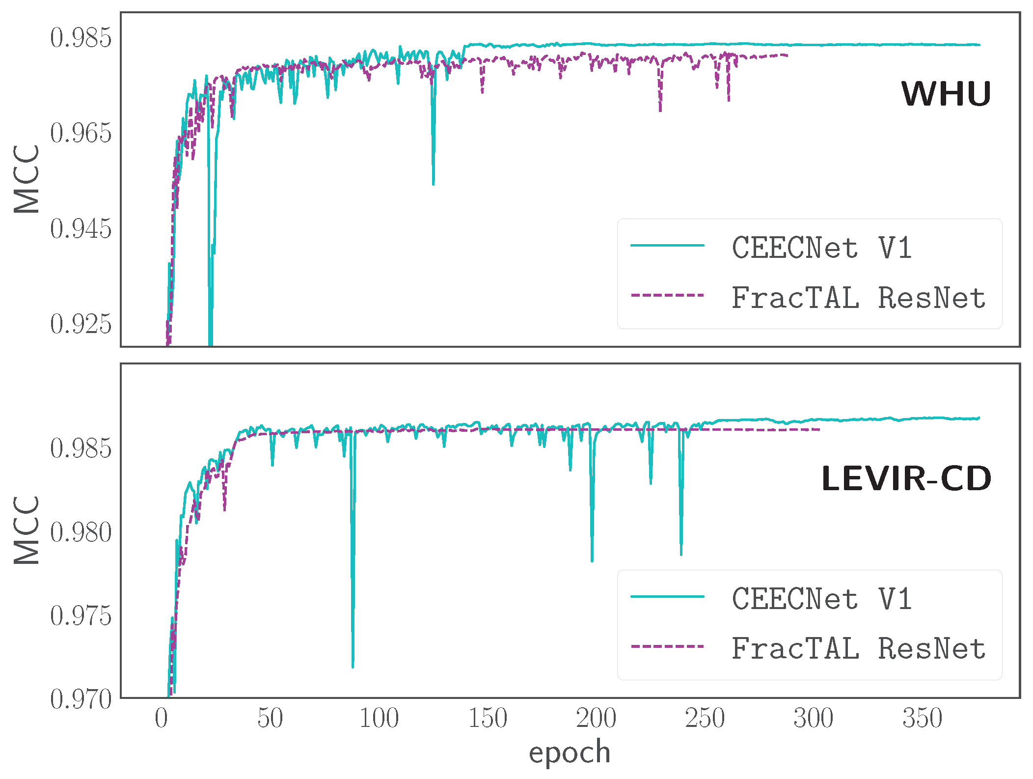
• We introduce a feature extraction building block that is based on the residual neural network [32] and the fractal Tanimoto Attention (Section 2.4.2). The new FracTALResNet converges faster to optimality than standard residual networks and enhances performance.
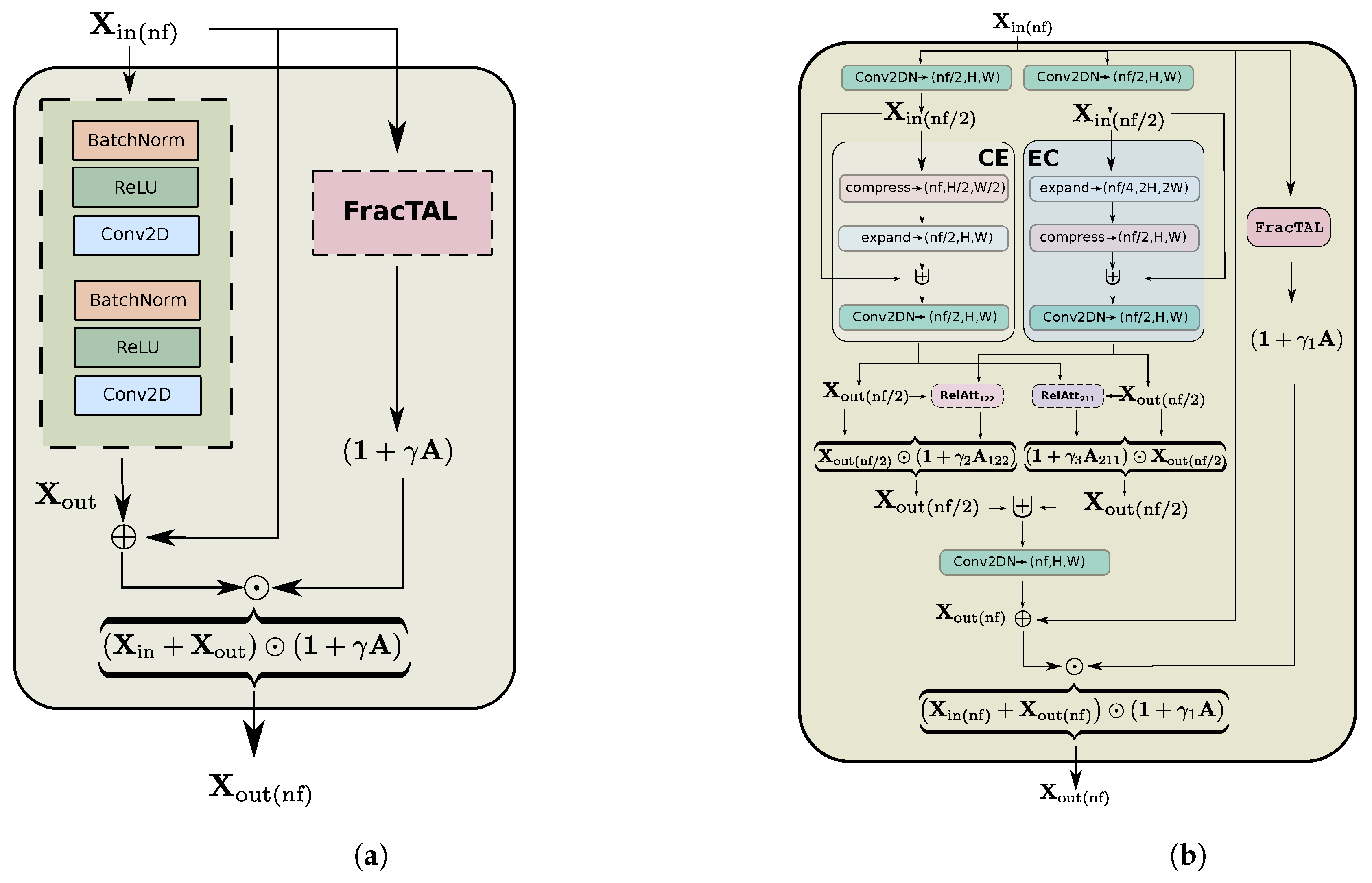
• We introduce two variants of a new feature extraction building block, the Compress-Expand/Expand-Compress unit (hereafter CEECNet unit—Section 2.5.1). This unit exhibits enhanced performance in comparison with standard residual units and the FracTALResNet unit.
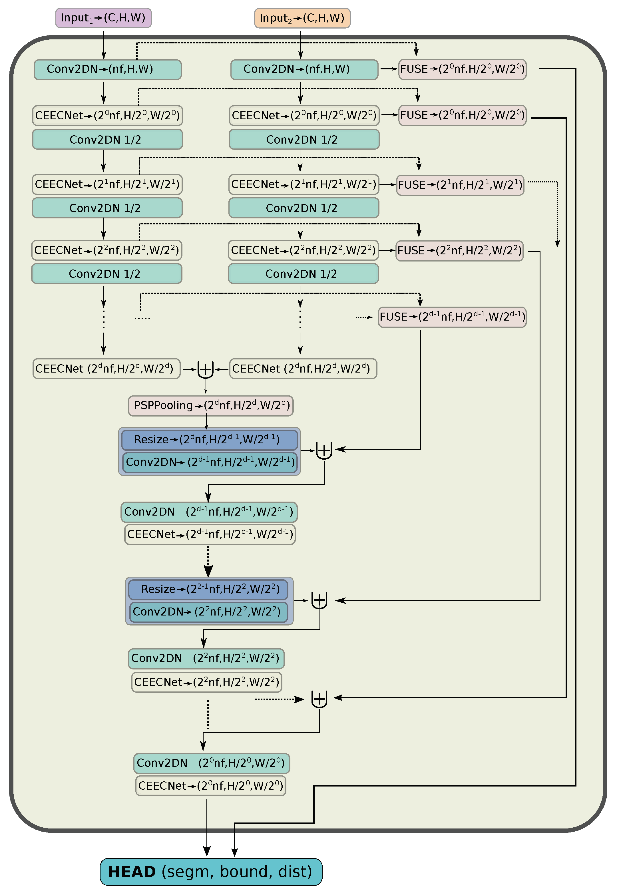
• Capitalising on these findings, we introduce a new backbone encoder/decoder scheme, a macro-topology—the mantis—that is tailored for the task of change detection (Section 2.5.2). The encoder part is a Siamese dual encoder, where the corresponding extracted features at each depth are fused together with FracTALrelative attention. In this way, information exchange between features extracted from bi-temporal images is enforced. There is no need for manual feature subtraction.
• Given the relative fusion operation between the encoder features at different levels, our algorithm achieves state-of-the-art performance on the LEVIRCD and WHU datasets without requiring the use of contrastive loss learning during training (Section 3.2). Therefore, it is easier to implement with standard deep learning libraries and tools.

Networks integrating the above-mentioned contributions yielded state-of-the-art performance for the task of building change detection in two benchmark datasets for change detection: the WHU [36] and LEVIRCD [1] datasets.

In addition to the previously mentioned sections, the following sections complete the work. In Section 2.6, we describe the setup of our experiments. In Section 3.1, we perform an ablation study of the proposed schemes. Finally, in Appendix C, we present various key elements of our architecture in mxnet/gluon style pseudocode. A software implementation of the models that relate to this work can be found on https://github.com/feevos/ceecnet, (accessed on 6 September 2020).

2. Materials and Methods

2.1. Fractal Tanimoto Similarity Coefficient

In [35], we analysed the performance of the various flavours of the Dice coefficient and introduced the Tanimoto with a complement coefficient. Here, we further expand our analysis, and we present a new functional form for this similarity metric. We use it both as a self-similarity measure between convolution layers in a new attention module and a loss function for fine-tuning semantic segmentation models.

For two (fuzzy) binary vectors of equal dimension, $\mathbf{p}$ and $\mathbf{l}$, whose elements lie in the range $(0,1)$, the Tanimoto similarity coefficient is defined:

$$T(\mathbf{p},\mathbf{l})=\frac{\mathbf{p}·\mathbf{l}}{{\mathbf{p}}^2+{\mathbf{l}}^2-\mathbf{p}·\mathbf{l}}$$

(1)

Interestingly, the dot product between two fuzzy binary vectors is another similarity measure of their agreement. This inspired us to introduce an iterative functional form of the Tanimoto:

$$\begin{array}{ccc}{\mathcal{T}}^0\hfill & \equiv \hfill & T(\mathbf{p},\mathbf{l})=\frac{\mathbf{p}·\mathbf{l}}{{\mathbf{p}}^2+{\mathbf{l}}^2-\mathbf{p}·\mathbf{l}}\hfill \end{array}$$

(2)

$$\begin{array}{ccc}{\mathcal{T}}^d\hfill & =\hfill & \frac{{\mathcal{T}}^{d-1}(\mathbf{p},\mathbf{l})}{{\mathcal{T}}^{d-1}(\mathbf{p},\mathbf{p})+{\mathcal{T}}^{d-1}(\mathbf{l},\mathbf{l})-{\mathcal{T}}^{d-1}(\mathbf{p},\mathbf{l})}\hfill \end{array}$$

(3)

For example, expanding Equation (2) for $d=2$, yields:

$${\mathcal{T}}^2(\mathbf{p},\mathbf{l})=\frac{\mathbf{p}·\mathbf{l}}{({\mathbf{l}}^2-\mathbf{p}·\mathbf{l}+{\mathbf{p}}^2)\left(2-\frac{\mathbf{p}·\mathbf{l}}{{\mathbf{l}}^2-\mathbf{p}·\mathbf{l}+{\mathbf{p}}^2}\right)\left(2-\frac{\mathbf{p}·\mathbf{l}}{({\mathbf{l}}^2-\mathbf{p}.\mathbf{l}+{\mathbf{p}}^2)\left(2-\frac{\mathbf{p}·\mathbf{l}}{{\mathbf{l}}^2-\mathbf{p}·\mathbf{l}+{\mathbf{p}}^2}\right)}\right)}$$

(4)

We can expand this for an arbitrary depth d, and then, we get the following simplified version of the fractal Tanimoto similarity measure:

$${\mathcal{T}}^d(\mathbf{p},\mathbf{l})=\frac{\mathbf{p}·\mathbf{l}}{2^d({\mathbf{p}}^2+{\mathbf{l}}^2)-(2^{d+1}-1)\mathbf{p}·\mathbf{l}}$$

(5)

This function (the simplified formula was obtained with Mathematica 11) takes values in the range $(0,1)$, and it becomes steeper as d increases. At the limit $d\to \infty$, it behaves like the integral of the Dirac $\delta$ function around point $\mathbf{l}$, $\int \delta (\mathbf{p}-\mathbf{l})d\mathbf{p}$. That is, the parameter d is a form of annealing “temperature”. Interestingly, although the iterative scheme was defined with d being an integer, for continuous values $d\ge 0$, ${\mathcal{T}}^d$ remains bounded in the interval $(0,1)$. That is:

$${\mathcal{T}}^d:{\Re }^n\times {\Re }^n\to U\subseteq [0,1]$$

(6)

where $n=dim\left(\mathbf{p}\right)$ is the dimensionality of the fuzzy binary vectors $\mathbf{p}$, $\mathbf{l}$.

In the following, we will use the functional form of the fractal Tanimoto with complement [35], i.e.:   

$${\mathcal{FT}}^d(\mathbf{p},\mathbf{l})\equiv \frac{{\mathcal{T}}^d(\mathbf{p},\mathbf{l})+{\mathcal{T}}^d(\mathbf{1}-\mathbf{p},\mathbf{1}-\mathbf{l})}{2}$$

(7)

In Figure 2, we provide a simple example for a ground truth vector $\mathbf{l}=\{0.4,0.6\}$ and a continuous vector of probabilities $\mathbf{p}=\{p_x,p_y\}$. On the top panel, we construct density plots of the Fractal Tanimoto function with complement ${\mathcal{FT}}^d$. The gradient field lines that point to the ground truth are overplotted. In the bottom panels, we plot the corresponding 3D representations. From left to right, the first column corresponds to $d=0$, the second to $d=3$, and the third to $d=5$. It is apparent that the effect of the d hyperparameter is to make the similarity metric steeper towards the ground truth. For all practical purposes (network architecture, evolving loss function), we use the average fractal Tanimoto loss (last column) due to having steeper gradients away from optimality. In order to avoid confusion between the depth d of the fractal Tanimoto loss function and the depth of the fractal Attention layer (introduced in Section 2.3), we will designate the depth of the loss function with the symbol $\mathfrak{D}$:

$${\langle \mathcal{FT}\rangle }^{\mathfrak{D}}(\mathbf{p},\mathbf{l})\equiv \frac{1}{\mathfrak{D}}\sum _{i=0}^{\mathfrak{D}-1}{\mathcal{FT}}^i(\mathbf{p},\mathbf{l})$$

(8)

The formula is valid for $\mathfrak{D}>=1$; for $\mathfrak{D}=0$, it reverts to the standard fractal Tanimoto loss: ${\mathcal{FT}}^{\mathfrak{D}=0}(\mathbf{p},\mathbf{l})$.

2.2. Evolving Loss Strategy

In this section, we describe a training strategy that modifies the depth of the fractal Tanimoto similarity coefficient, when used as a loss function, on each learning rate reduction. For minimisation problems, the fractal Tanimoto loss is defined through: $L^{\mathfrak{D}}=1-{\langle \mathcal{FT}\rangle }^{\mathfrak{D}}$. In the following, when we refer to the fractal Tanimoto loss function, it should be understood that this is defined through the similarity coefficient, as described above.

During training and until the first learning rate reduction, we use the standard Tanimoto with complement ${\mathcal{FT}}^0(\mathbf{p},\mathbf{l})$. The reason for this is that for a random initialization of the weights (i.e., for an initial prediction point in the space of probabilities away from optimality), the gradients are steeper towards the best values for this particular loss function (in fact, for cross entropy are even steeper). This can be seen in Figure 2 in the bottom row: clearly, for an initial probability vector $\mathbf{p}=\{p_x,p_y\}$ away from the ground truth $\mathbf{l}=\{0.4,0.6\}$, the gradients are steeper for $\mathfrak{D}=0$. As training evolves, and the value of the weights approaches optimality, the predictions approach the ground truth, and the loss function flattens out. With batch gradient descent (and variants), we are not really calculating the true (global) loss function but rather a noisy approximate version of it. This is because in each batch loss evaluation, we are not using all of the data for the gradients evaluation. In Figure 3, we represent a graphical representation of the true landscape and a noisy version of it for a toy 2D problem. In the top row, we plot the value of the ${\mathcal{FT}}^0$ similarity as well as the average value of the loss functions for $\mathfrak{D}=0,\dots ,9$ for the ground truth vector $\mathbf{l}=\{0.4,0.6\}$. In the corresponding bottom rows, we have the same plot, where we also added random Gaussian noise. In the initial phases of training, the average gradients are greater than the local values due to noise. As the network reaches optimality, the average gradient towards optimality becomes smaller and smaller, and the gradients due to noise dominate the training. Once we reduce the learning rate, the step the optimiser takes is even smaller; therefore, it cannot easily escape local optima (due to noise). What we propose is to “shift gears”: once training stagnates, we change the loss function to a similar but steeper one towards optimality that can provide gradients (on average) that can dominate the noise. Our choice during training is the following set of learning rates and depths of the fractal Tanimoto loss: $\{(\mathtt{lr}:{10}^{-3},\mathfrak{D}=0),(\mathtt{lr}:{10}^{-4},\mathfrak{D}=10),(\mathtt{lr}:{10}^{-5},\mathfrak{D}=20)\}$. In all evaluations of loss functions for $\mathfrak{D}>0$, we use the average value for all $\mathfrak{D}$ values (Equation (8)).

2.3. Fractal Tanimoto Attention

Here, we present a novel convolutional attention layer based on the new similarity metric and a methodology of fusing information from the output of the attention layer to features extracted from convolutions.

2.4. Fractal Tanimoto Attention Layer

In the pioneering work of [14], the attention operator is defined through a scaled dot product operation. For images, in particular, i.e., two-dimensional features, assuming that $\mathbf{q}\in {\mathfrak{R}}^{C_q\times H\times W}$ is the query, $\mathbf{k}\in {\mathfrak{R}}^{C\times H\times W}$ the key, and $\mathbf{v}\in {\mathfrak{R}}^{C\times H\times W}$ its corresponding value, the (spatial) attention is defined as (see also [37]):

$$\begin{array}{cccc}\hfill \mathbf{o}& =\mathrm{softmax}\left(\frac{\mathbf{q}{\circ }_1\mathbf{k}}{\sqrt{d}}\right),\hfill & \hfill & \in {\mathfrak{R}}^{C_q\times C}\hfill \end{array}$$

(9)

$$\begin{array}{cccc}\hfill \mathrm{Att}(\mathbf{q},\mathbf{k},\mathbf{v})& =\mathbf{o}{\circ }_2\mathbf{v},\hfill & \hfill & \in {\mathfrak{R}}^{C_q\times H\times W}\hfill \end{array}$$

(10)

Here d is the dimension of the keys, and the softmax operation is with respect to the first (channel) dimension. The term $\sqrt{d}$ is a scaling factor that ensures the Attention layer scales well even with a large number of dimensions [14]. The operator ${\circ }_1$ corresponds to the inner product with respect to the spatial dimensions height, H, and width, W, while ${\circ }_2$ is a dot product with respect to channel dimensions. This is more apparent in index notation:

$$\begin{array}{cc}\hfill \mathbf{q}{\circ }_1\mathbf{k}& \equiv \sum _{jk}{q}_{ijk}{k}_{ljk}\in {\mathfrak{R}}^{C_q\times C}\hfill \\ \hfill \mathbf{o}& \equiv \mathrm{softmax}\left(\mathbf{q}{\circ }_1\mathbf{k}\right)\equiv o_{il}\hfill \\ \hfill \mathrm{Att}(\mathbf{q},\mathbf{k},\mathbf{v})& \equiv {\mathrm{Att}}_{ikj}\equiv \mathbf{o}{\circ }_2\mathbf{v}\equiv \sum _l{o}_{il}{v}_{lkj}\in {\mathfrak{R}}^{C_q\times H\times W}\hfill \end{array}$$

(11)

In this formalism, each channel of the query features is compared with each of the channels of the key values. In addition, there is a 1-1 correspondence between keys and values, meaning that a unique value corresponds to each key. The point of the dot product is to emphasise the key-value pairs that are more relevant for the particular query. That is the dot product selects the keys that are most similar to the particular query. It represents the projection of queries on the keys space. The softmax operator provides a weighted “view” of all the values for a particular set of queries, keys, and values or else a “soft” attention mechanism. In the multi-head attention paradigm, multiple attention heads that follow the principles described above are concatenated together. One of the key disadvantages of this formulation when used in vision tasks (i.e., two dimensional features) is the very large memory footprint that this layer exhibits. For 1D problems, such as Natural Language Processing, this is not an issue in general.

Here, we follow a different approach. We develop our formalism for the case where the number of query channels, $C_q$, is identical to the number of key channels, C. However, if desired, our formalism can work for the general case where $C_q\ne C$.

Let $\mathbf{q}\in {\mathfrak{R}}^{C\times H\times W}$ be the query features, $\mathbf{k}\in {\mathfrak{R}}^{C\times H\times W}$ the keys, and $\mathbf{v}\in {\mathfrak{R}}^{C\times H\times W}$ the values. In our formalism, it is a requirement for these operators to have values in $[0,1]$. This can be easily achieved by applying the sigmoid operator. Our approach is a joint spatial and channel attention mechanism. With the use of the Fractal Tanimoto similarity coefficient, we define the spatial, ⊠, and channel, ⊡, similarity between the query, $\mathbf{q}$, and key, $\mathbf{k}$, features according to:

$$\begin{array}{c}\hfill {\mathcal{T}}_{⊠}^d(\mathbf{q},\mathbf{k})=\frac{\mathbf{q}⊠\mathbf{k}}{2^d\left(\mathbf{q}⊠\mathbf{q}+\mathbf{k}⊠\mathbf{k}\right)-(2^{d+1}-1)\mathbf{q}⊠\mathbf{k}}\in {\mathfrak{R}}^C\end{array}$$

(12)

$$\begin{array}{c}\hfill {\mathcal{T}}_{⊡}^d(\mathbf{q},\mathbf{k})=\frac{\mathbf{q}⊡\mathbf{k}}{2^d\left(\mathbf{q}⊡\mathbf{q}+\mathbf{k}⊡\mathbf{k}\right)-(2^{d+1}-1)\mathbf{q}⊡\mathbf{k}}\in {\mathfrak{R}}^{H\times W}\end{array}$$

(13)

where the spatial and channel products are defined as:   

$$\begin{array}{cc}\hfill \mathbf{q}⊠\mathbf{k}& =\sum _{jk}{q}_{ijk}{k}_{ijk}\in {\mathfrak{R}}^C\hfill \\ \hfill \mathbf{q}⊡\mathbf{k}& =\sum _i{q}_{ijk}{k}_{ijk}\in {\mathfrak{R}}^{H\times W}\hfill \end{array}$$

It is important to note that the output of these operators lies numerically within the range (0, 1), where 1 indicates identical similarity and 0 indicates no correlation between the query and key. That is, there is no need for normalisation or scaling as is the case for the traditional dot product similarity.

In our approach, the spatial and channel attention layers are defined with element-wise multiplication (denoted by the symbol ⊙):

$$\begin{array}{cc}\hfill {\mathrm{Att}}_{⊠}(\mathbf{q},\mathbf{k},\mathbf{v})& ={\mathcal{T}}_{⊠}^d(\mathbf{q},\mathbf{k})\odot \mathbf{v}\hfill \\ \hfill {\mathrm{Att}}_{⊡}(\mathbf{q},\mathbf{k},\mathbf{v})& ={\mathcal{T}}_{⊡}^d(\mathbf{q},\mathbf{k})\odot \mathbf{v}\hfill \end{array}$$

It should be stressed that these operations do not consider that there is a 1-1 mapping between keys and values. Instead, we consider a map of one-to-many; that is, a single key can correspond to a set of values. Therefore, there is no need to use a softmax activation (see also [38]). The overall attention is defined as the average of the sum of these two operators:

$$\mathrm{Att}(\mathbf{q},\mathbf{k},\mathbf{v})=0.5({\mathrm{Att}}_{⊠}+{\mathrm{Att}}_{⊡})$$

(14)

In practice, we use the averaged fractal Tanimoto similarity coefficient with complement, ${\langle \mathcal{FT}\rangle }_{⊠/⊡}^d$, both for spatial and channel wise attention.

As stated previously, it is possible to extend the definitions of spatial and channel products in a way where we compare each of the channels (respectively, spatial pixels) of the query with each of the channels (respectively, spatial pixels) of the key. However, this imposes a heavy memory footprint and makes deeper models, even for modern-day GPUs, prohibitive. This will be made clear with an example of FracTALspatial similarity vs. the dot product similarity that appears in SAGAN [39] self-attention. Let us assume that we have an input feature layer of size $(B\times C\times H\times W)=32\times 1024\times 16\times 16$ (e.g., this appears in the layer at depth 6 of UNet-like architectures, starting from 32 initial features). From this, three layers are produced of the same dimensionalty, the query, the key, and value. With the Fractal Tanimoto spatial similarity, ${\mathcal{T}}_{⊠}$, the output of the similarity of query and keys is $B\times C\times 1\times 1=32\times 1024\times 1\times 1$ (Equation (12)). The corresponding output of the dot similarity of spatial compoments in the self-attention is $B\times C\times C$ → $32\times 1024\times 1024$ (Equation (11)), having a C-times higher memory footprint.

In addition, we found that this approach did not improve the performance for the case of change detection and classification. Indeed, one needs to question this for vision tasks: the initial definition of attention [12] introduced a relative alignment vector, $e_{ij}$, that was necessary because, for the task of NMT, the syntax of phrases changes from one language to the other. That is, the relative emphasis with respect to location between two vectors is meaningful. When we compare two images (features) at the same depth of a network (created by two different inputs, as is the case for change detection), we anticipate that the channels (or spatial pixels) will be in correspondence. For example, the RGB (or hyperspectral) order of inputs, does not change. That is, in vision, the situation can be different than NLP because we do not have a relative location change as it happens with words in phrases.

We propose the use of the Fractal Tanimoto Attention Layer (hereafter FracTAL) for vision tasks as an improvement over the scaled dot product attention mechanism [14] for the following reasons:

• The $\mathcal{FT}$ similarity is automatically scaled in the region $(0,1)$; therefore, it does not require normalisation or activation to be applied. This simplifies the design and implementation of Attention layers and enables training without ad hoc normalisation operations.
• The dot product does not have an upper or lower bound; therefore, a positive value cannot be a quantified measure of similarity. In contrast, $\mathcal{FT}$ has a bounded range of values in $(0,1)$. The lowest value indicates no correlation, and the maximum value perfect similarity. It is thus easier to interpret.
• Iteration d is a form of hyperparameter, such as “temperature” in annealing. Therefore, the $\mathcal{FT}$ can become as steep as we desire (by modification of the temperature parameter d), even steeper than the dot product similarity. This can translate to finer query and key similarity.
• Finally, it is efficient in terms of the GPU memory footprint (when one considers that it does both channel and spatial attention), thus allowing the design of more complex convolution building blocks.

The implementation of the FracTALis given in

Listing A.2. mxnet/gluon style pseudocode for the fractal Tanimoto Attention module.

from mxnet import nd as F from mxnet.gluon import nn class FTAttention2D(nn.Block):     def __init__(self, nchannels, nheads, **kwards):             super().__init__(**kwards)         self.q = Conv2DN(nchannels,groups=nheads)         self.k = Conv2DN(nchannels,groups=nheads)         self.v = Conv2DN(nchannels,groups=nheads)         # spatial/channel similarity         self.SpatialSim = FTanimoto(axis=[2,3])         self.ChannelSim = FTanimoto(axis=1)         self.norm = nn.BatchNorm()       def forward(self, qin, kin, vin):         # query, key, value         q = F.sigmoid(self.q(qin))#dim:(B,C,H,W)         k = F.sigmoid(self.k(vin))#dim:(B,C,H,W)         vs. = F.sigmoid(self.v(kin))#dim:(B,C,H,W)           att_spat = self.ChannelSim(q,k)#dim:(B,1,H,W)         v_spat  =  att_spat*v #dim:(B,C,H,W)           att_chan = self.SpatialSim(q,k)#dim:(B,C,1,1)         v_chan   = att_chan*v #dim:(B,C,H,W)           v_cspat =  0.5*(v_chan+v_spat)         v_cspat = self.norm(v_cspat)           return v_cspat #dim:(B,C,H,W)

. The multihead attention is achieved using group convolutions for the evaluation of queries, keys, and values.

2.4.1. Attention Fusion

A critical part in the design of convolution building blocks enhanced with attention is the way the information from attention is passed to convolution layers. To this aim, we propose fusion methodologies of feature layers with the FracTAL for two cases: self attention fusion and a relative attention fusion, where information from two layers are combined.

2.4.2. Self Attention Fusion

We propose the following fusion methodology between a feature layer, $\mathbf{L}$, and its corresponding FracTALself-attention layer, $\mathbf{A}$:

$$\mathbf{F}=\mathbf{L}+\gamma \mathbf{L}\odot \mathbf{A}=\mathbf{L}\odot (\mathbf{1}+\gamma \mathbf{A})$$

(15)

Here, $\mathbf{F}$ is the output layer produced from the fusion of $\mathbf{L}$ and the Attention layer, $\mathbf{A}$, ⊙ describes element wise multiplication, $\mathbf{1}$ is a layer of ones such as L, and $\gamma$ a trainable parameter initiated at zero. We next describe the reasons why we propose this type of fusion.

The Attention output is maximal (i.e., close to 1) in areas on the features where it must “attend” and minimal otherwise (i.e., close to zero). Directly multiplying element-wise the FracTALattention layer $\mathbf{A}$ with the features, $\mathbf{L}$, effectively lowers the values of features in areas that are not “interesting”. It does not alter the value of areas that “are interesting”. This can produce loss of information in areas where $\mathbf{A}$ “does not attend” (i.e., it does not emphasize), which would otherwise be valuable at a later stage. Indeed, areas of the image that the algorithm “does not attend” should not be perceived as empty space [11]. For this reason, the “emphasised” features, $\mathbf{L}\odot \mathbf{A}$, are added to the original input $\mathbf{L}$. Moreover, $\mathbf{L}+\mathbf{L}\odot \mathbf{A}$ is identical to $\mathbf{L}$ in spatial areas where $\mathbf{A}$ tends to zero and is emphasised in areas where $\mathbf{A}$ is maximal.

In the initial stages of training, the attention layer, $\mathbf{A}$, does not contribute to $\mathbf{L}$ due to the initial value of the trainable parameter ${\gamma }_0=0$. Therefore, it does not add complexity during the initial phase of training, and it allows for an annealing process of the Attention contribution (see also [31,39]). This property is particularly important when $\mathbf{L}$ is produced from a known performant recipe (e.g., residual building blocks).

In Figure 4a, we present this fusion mechanism for the case of a Residual unit [32,40]. Here, the input layer, ${\mathbf{X}}_{\mathrm{in}}$, is subject to the residual block sequence of Batch normalisation, convolutions, and ReLU activations and produces the ${\mathbf{X}}_{\mathrm{out}}$ layer. A separate branch uses the ${\mathbf{X}}_{\mathrm{in}}$ input to produce the self attention layer $\mathbf{A}$ (see Listing A.2). Then we multiply element-wise the standard output of the residual unit, ${\mathbf{X}}_{\mathrm{in}}+{\mathbf{X}}_{\mathrm{out}}$, with the $\mathbf{1}+\gamma \mathbf{A}$ layer. In this way, at the beginning of training, this layer behaves as a residual layer, which has excellent convergent properties of resnet at initial stages, and at later stages of training, the Attention becomes gradually more active and allows for greater performance. A software routine of this fusion for the residual unit, in particular, can be seen in

Listing A.4. mxnet/gluon style pseudocode for the Residual Attention Fusion module.

import mxnet as mx from mxnet import nd as F class FTAttResUnit(nn.Block):     def __init__(self, nchannels, nheads, **kwards):         super().__init__(**kwards)         # Residual Block: sequence of         # (BN,ReLU,Conv,BN,ReLU,Conv)         self.ResBlock = ResBlock(nchannels,                           kernel=3,                           padding=1)         self.att = FTAttention2D(nchannels,nheads)           self.gamma  = self.params.get(’gamma’,                       shape=(1,),                       init=mx.init.Zero())       def forward(self, input):         out = self.ResBlock(input)#dim:(B,C,H,W)         qin = input         vin = input         kin = input         att = self.attention(qin,vin,kin)#dim:(B,C,H,W)         att = self.gamma * att         out = (input + out)*(F.ones_like(out)+att)         return out

in the Appendix C.

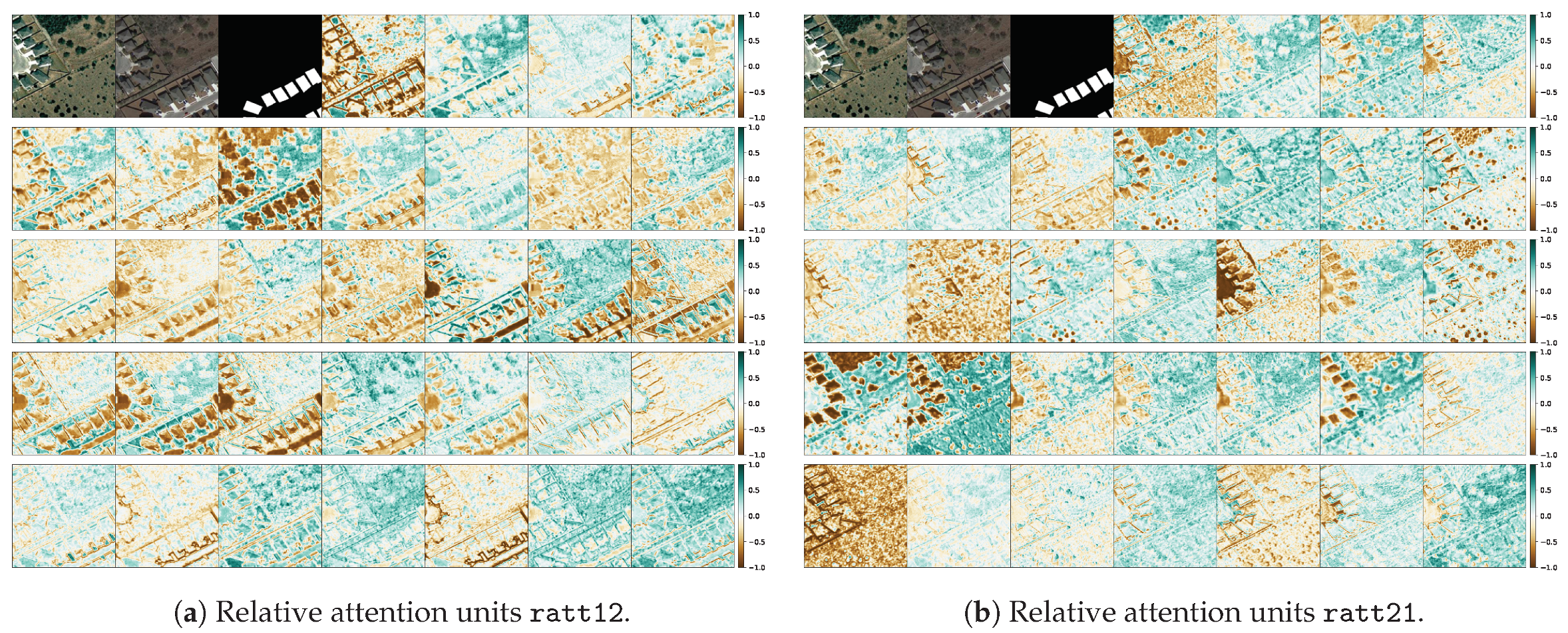
2.4.3. Relative Attention Fusion

Assuming we have two input layers, ${\mathbf{L}}_1$ and ${\mathbf{L}}_2$, we can calculate the relative attention of each with respect to the other. This is achieved by using the layer we want to “attend to” as query and the layer we want to use as information for attention as a key and value. In practical implementations, the query, the key, and the value layers result after the application of a convolution layer to some input.

$$\begin{array}{cc}\hfill {\mathbf{F}}_1& ={\mathbf{L}}_1\odot \left[\mathbf{1}+{\gamma }_1{\mathbf{A}}_{122}(\mathbf{q}\left({\mathbf{L}}_1\right),\mathbf{k}\left({\mathbf{L}}_2\right),\mathbf{v}\left({\mathbf{L}}_2\right))\right]\hfill \end{array}$$

(16)

$$\begin{array}{cc}\hfill {\mathbf{F}}_2& ={\mathbf{L}}_2\odot [\mathbf{1}+{\gamma }_2{\mathbf{A}}_{211}(\mathbf{q}\left({\mathbf{L}}_2\right),\mathbf{k}\left({\mathbf{L}}_1\right),\mathbf{v}\left({\mathbf{L}}_1\right))]\hfill \end{array}$$

(17)

$$\begin{array}{cc}\hfill \mathbf{F}& =\mathrm{Conv}2\mathrm{DN}\left(\mathrm{concat}\left([{\mathbf{F}}_1,{\mathbf{F}}_2]\right)\right)\hfill \end{array}$$

(18)

Here, the ${\gamma }_{1,2}$ parameters are initialized at zero, and the concatenation operations are performed along the channel dimension. Conv2DN is a two-dimensional convolution operation followed by a normalisation layer, e.g., BatchNorm [41]). An implementation of this process in mxnet/gluon pseudocode style can be found in

Listing A.3. mxnet/gluon style pseudocode for the Relative Attention Fusion module.

import mxnet as mx from mxnet import nd as F class Fusion(nn.Block):     def __init__(self, nchannels, nheads, **kwards):         super().__init__(**kwards)         self.fuse = Conv2DN(nchannels,                           kernel=3,                           padding=1,                           groups=nheads)         self.att12 = FTAttention2D(nchannels,nheads)         self.att21 = FTAttention2D(nchannels,nheads)           self.gamma1  = self.params.get(’gamma1’,                       shape=(1,),                       init=mx.init.Zero())         self.gamma2  = self.params.get(’gamma2’,                       shape=(1,),                       init=mx.init.Zero())       def forward(self, input1,input2):         ones = nd.ones_like(input1)           # Attention on 1, for k,v from 2         qin = input1         kin = input2         vin = input2         att12 = self.att12(qin,kin,vin)         out12 = input1*(ones+self.gamma1*att12)           # Attention on 2, for k,v from 1         qin = input2         kin = input1         vin = input1         att21 = self.att21(qin,kin,vin)      out21 = input2*(ones+self.gamma2*att21)        out = nd.concat(out12,out21,dim=1)      out = self.fuse(out)             return out

.

The relative attention fusion presented here can be used as a direct replacement of concatenation followed by a convolution layer in any network design.

2.5. Architecture

We break down the network architecture into three component parts: the micro-topology of the building blocks, which represents the fundamental constituents of the architecture; the macro-topology of the network, which describes how building blocks are connected to one another to maximise performance; and the multitasking head, which is responsible for transforming the features produced by the micro- and macro-topologies into the final prediction layers where change is identified. Each of the choices of micro- and macro-topology has a different impact on the GPU memory footprint. Usually, selecting very deep macro-topology improves performance, but then this increases the overall memory footprint and does not leave enough space for using an adequate number of filters (channels) in each micro-topology. There is obviously a trade off between the micro-topology feature extraction capacity and the overall network depth. Guided by this, we seek to maximise the feature expression capacity of the micro-topology for a given number of filters, perhaps at the expense of consuming computational resources.

2.5.1. Micro-Topology: The CEECNet Unit

The basic intuition behind the construction of the CEEC building block is that it provides two different, yet complementary, views for the same input. The first view (the CE block—see Figure 4b) is a “summary understanding” operation (performed in lower resolution than the input—see also [42,43,44]). The second view (the EC block) is an “analysis of detail” operation (performed in higher spatial resolution than the input). It then exchanges information between these two views using relative attention, and it finally fuses them together by emphasising the most important parts using the FracTAL.

Our hypothesis and motivation for this approach is quite similar to the scale-space analysis in computer vision [45]: viewing input features at different scales allows the algorithm to focus on different aspects of the inputs and thus perform more efficiently. The fact that by merely increasing the resolution of an image, its content information does not increase is not relevant here: guided by the loss function, the algorithm can learn to represent at higher resolution features that otherwise would not be possible in lower resolutions. We know this from the successful application of convolutional networks in super-resolution problems [46] as well as (variational) autoencoders [47,48]: in both of these paradigms, deep learning approaches manage to meaningfully increase the resolution of features that exist in lower spatial dimension layers.

In the following, we define the volume V of features of dimension $(C,H,W)$ as the product of the number of their channels (or filters), C (or $nf$), with their spatial dimensions, height, H, and width, W, i.e., $V=nf·H·W$. Here, C is the number of channels, H and W the spatial dimensions, height and width, respectively. For example, for each batch dimension, the output volume of a layer of size $(C,H,W)=(32,256,256)$ is $V=32\times {256}^2=2097152$. The two branches consist of: a “mini ∪-Net” operation (CE block), which is responsible for summarising information from the input features by first compressing the total volume of features into half its original size and then restoring it. The second branch, a “mini ∩-Net” operation (EC block), is responsible for analysing the input features in higher detail: it initially doubles the volume of the input features by halving the number of features and doubling each spatial dimension. It subsequently compresses this expanded volume to its original size. The input to both layers is concatenated with the output, and then a normed convolution restores the number of channels to their original input value. Note that the mini ∩-Net is nothing more than the symmetric (or dual) operation of the mini ∪-Net.

The outputs of the EC and CE blocks are fused together with relative attention fusion (Section 2.4.3). In this way, the exchange of information between the layers is encouraged. The final emphasised outputs are concatened together, thus restoring the initial number of filters, and the produced layer is passed through a normed convolution in order to bind the relative channels. The operation is concluded with a FracTALresidual operation and fusion (similar to Figure 4a), where the input is added to the final output and emphasised by the self attention on the original input. The CEECNet building block is described schematically in Figure 4b.

The compression operation, C, is achieved by applying a normed convolution layer of stride equal to 2 (k = 3, p = 1, s = 2) followed by another convolution layer that is identical in every aspect, except the stride that is now s = 1. The purpose of the first convolution is to both resize the layer and extract features. The purpose of the second convolution layer is to extract features. The expansion operation, E, is achieved by first resizing the spatial dimensions of the input layer using Bilinear interpolation, and then the number of channels is brought to the desired size by the application of a convolution layer (k = 3, p = 1, s = 1). Another identical convolution layer is applied to extract further features. The full details of the convolution operations used in the EC and CE blocks can be found on

Listing A.5. mxnet/gluon style pseudocode for the CEECNetV1 unit.

import mxnet as mx from mxnet import nd as F class CEECNet_unit_V1(nn.Block):     def __init__(self, nchannels, nheads, **kwards):         super().__init__(**kwards)         # Compress-Expand         self.conv1= Conv2DN(nchannels/2)         self.compr11= Conv2DN(nchannels,k=3,p=1,s=2)         self.compr12= Conv2DN(nchannels,k=3,p=1,s=1)         self.expand1= ExpandNComb(nchannels/2)           # Expand Compress         self.conv2= Conv2DN(nchannels/2)         self.expand2= Expand(nchannels/4)         self.compr21= Conv2DN(nchannels/2,k=3,p=1,s=2)         self.compr22= Conv2DN(nchannels/2,k=3,p=1,s=1)           self.collect= Conv2DN(nchannels,k=3,p=1,s=1)           self.att= FTAttention2D(nchannels,nheads)         self.ratt12= RelFTAttention2D(nchannels,nheads)         self.ratt21= RelFTAttention2D(nchannels,nheads)             self.gamma1  = self.params.get(’gamma1’,                       shape=(1,),                       init=mx.init.Zero())         self.gamma2  = self.params.get(’gamma2’,                       shape=(1,),                       init=mx.init.Zero())         self.gamma3  = self.params.get(’gamma3’,                       shape=(1,),                       init=mx.init.Zero())       def forward(self, input):         # Compress-Expand      out10 = self.conv1(input)      out1  = self.compr11(out10)      out1  = F.relu(out1)      out1  = self.compr12(out1)      out1  = F.relu(out1)      out1  = self.expand1(out1,out10)      out1  = F.relu(out1)        # Expand-Compress      out20 = self.conv2(input)      out2  = self.expand2(out20)      out2  = F.relu(out2)      out2  = self.compr21(out2)      out2  = F.relu(out2)      out2  = F.concat([out2,out20],axis=1)      out2  = self.compr22(out2)          out2  = F.relu(out2)           # attention      att   = self.gamma1*self.att(input)           # relative attention 122      qin   = out1         kin   = out2         vin   = out2         ratt12 = self.gamma2*self.ratt12(qin,kin,vin)           # relative attention 211         qin   = out2         kin   = out1         vin   = out1         ratt21 = self.gamma3*self.ratt21(qin,kin,vin)        ones1 = F.ones_like(out10)# nchannels/2        out122= out1*(ones1+ratt12)      out211= out2*(ones1+ratt21)         out12 = F.concat([out122,out211],dim=1)         out12 = self.collect(out12)         out12 = F.relu(out12)         # Final fusion         ones2 = F.ones_like(input)         out   = (input+out12)*(ones2+att)         return out

.

2.5.2. Macro-Topology: Dual Encoder, Symmetric Decoder

In this section, we present the macro-topology (i.e., backbone) of the architecture that uses either the CEECNet or the FracTALResNet units as building blocks. We start by stating the intuition behind our choices and continue with a detailed description of the macro-topology. Our architecture is heavily influenced by the ResUNet-a model [35]. We will refer to this macro-topology as the mantis topology.

In designing this backbone, a key question we tried to address is how we can facilitate exchange of information between features extracted from images at different dates. The following two observations guided us:

• We make the hypothesis that the process of change detection between two images requires a mechanism similar to human attention. We base this hypothesis on the fact that the time required for identifying objects that changed in an image correlates directly with the number of changed objects. That is, the more objects a human needs to identify between two pictures, the more time is required. This is in accordance with the feature-integration theory of Attention [11]. In contrast, subtracting features extracted from two different input images is a process that is constant in time, independent of the complexity of the changed features. Therefore, we avoid using ad hoc feature subtraction in all parts of the network.
• In order to identify change, a human needs to look and compare two images multiple times, back and forth. We need things to emphasise on image at date 1, based on information on image at date 2 (Equation (16)) and, vice versa, (Equation (17)). Furthermore, then we combine both of these pieces of information together (Equation (18)). That is, exchange information with relative attention (Section 2.4.3) between the two at multiple levels. A different way of stating this as a question is: what is important on input image 1 based on information that exists on image 2, and vice versa?

Given the above, we now proceed in detailing the mantis macro-topology (with CEECNetV1 building blocks, see Figure 5). The encoder part is a series of building blocks, where the size of the features is downscaled between the application of each subsequent building block. Downscaling is achieved with a normed convolution with stride, s = 2, without using activations. There exist two encoder branches that share identical parameters in their convolution layers. The input to each branch is an image from a different date, and the role of the encoder is to extract features at different levels from each input image. During the feature extraction by each branch, each of the two inputs is treated as an independent entity. At successive depths, the outputs of the corresponding building block are fused together with the relative attention methodology, as described in Section 2.4.3, but they are not used until later in the decoder part. Crucially, this fusion operation suggests to the network that the important parts of the first layer will be defined by what exists on the second layer (and vice versa), but it does not dictate how exactly the network should compare the extracted features (e.g., by demanding the features to be similar for unchanged areas, and maximally different for changed areas—we tried this approach, and it was not successful). This is something that the network will have to discover in order to match its predictions with the ground truth. Finally, the last encoder layers are concatenated and inserted into the pyramid scene pooling layer (PSPPooling—[35,49]).

In the (single) decoder part, the network extracts features based on the relative information that exist in the two inputs. Starting from the output of the PSPPooling layer (middle of network), we upscale lower resolution features with bilinear interpolation and combine them with the fused outputs of the decoder with a concatenation operation followed by a normed convolution layer, in a way similar to the ResUNet-a [35] model. The mantis CEECNetV2 model replaces all concatenation operations followed by a normed convolution with a Fusion operation, as described in Listing A.3.

The final features extracted from this macro-topology architecture is the final layer from the CEECNet unit that has the same spatial dimensions as the first input layers, as well as the Fused layers from the first CEECNet unit operation. Both of these layers are inserted into the segmentation HEAD.

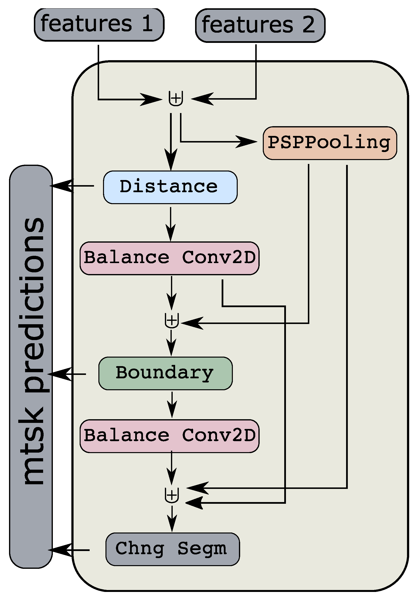
2.5.3. Segmentation HEAD

The features extracted from the features extractor (Figure 5) are inserted into a conditioned multitasking segmentation head (Figure 6) that produces three layers: a segmentation mask, a boundary mask, and a distance transform mask. This is identical with the ResUNet-a “causal” segmentation head, which has shown great performance in a variety of segmentation tasks [35,50], with two modifications.

The first modification relates to the evaluation of boundaries: instead of using a standard sigmoid activation for the boundaries layer, we are inserting a scaling parameter, $\gamma$, that controls how sharp the transition from 0 to 1 takes place, i.e.,

$${\mathtt{sigmoid}}_{\mathrm{crisp}}\left(x\right)=\mathtt{sigmoid}(x/\gamma ),\gamma \in [ϵ,1]$$

(19)

Here $ϵ={10}^{-2}$ is a smoothing parameter. The $\gamma$ coefficient is learned during training. We inserted this scaling after noticing in initial experiments that the algorithm needed improvement close to the boundaries of objects. In other words, the algorithm was having difficulty separating nearby pixels. Numerically, we anticipate that the distance between the values of activations of neighbouring pixels is small due to the patch-wise nature of convolutions. Therefore, a remedy to this problem is making the transition boundary sharper. We initialise training with $\gamma =1$.

The second modification to the segmentation HEAD relates to balancing the number of channels of the boundaries and distance transform predictions before re-using them in the final prediction of segmentation change detection. This is achieved by passing them through a convolution layer that brings the number of channels to the desired number. Balancing the number of channels treats the input features and the intermediate predictions as equal contributions to the final output. In Figure 6, we present schematically the conditioned multitasking head and the various dependencies between layers. Interested users can refer to [35] for details on the conditioned multitasking head.

2.6. Experimental Design

In this section, we describe the setup of our experiments for the evaluation of the proposed algorithms on the task of change detection. We start by describing the two datasets we used (LEVIRCD [1] and WHU [36]) as well as the data augmentation methodology we followed. Then we proceed in describing the metrics used for performance evaluation and the inference methodology. All models mantis CEECNetV1, V2, and mantis FracTAL ResNet have an initial number of filters equal to nf = 32, and the depth of the encoder branches was equal to 6. We designate these models with D6nf32.

2.6.1. LEVIRCD Dataset

The LEVIR-CD change detection dataset [1] consists of 637 pairs of VHR aerial images of resolution 0.5 m per pixel. It covers various types of buildings, such as villa residences, small garages, apartments, and warehouses. It contains 31,333 individual building changes. The authors provide a train/validation/test split, which standardises the performance process. We used a different split for training and validation; however, we used the test set the authors provide for reporting performance. For each tile from the training and validation set, we used ∼47% of the area for training and the remaining ∼53% for validation. For a rectangle area with sides of length a and b, this is achieved by using as training area the rectangle with sides $a^{\prime }=0.6838a$ and $b^{\prime }=0.6838b$, i.e., $\mathtt{training\; area}={0.6838}^{2}ab\approx 0.47ab$. Then $\mathtt{val\; area}=1.-\mathtt{train\; area}\approx 0.53\mathtt{total\; area}$. From each of these areas, we extracted chips of size $256\times 256$. These are overlapping in each dimension with stride equal to $256/2=128$ pixels.

2.6.2. WHU Building Change Detection

The WHU building change dataset [36] consists of two aerial images (2011 and 2016) that cover an area of ∼20 km${}^2$, which was changed from 2011 (earthquake) to 2016. The images resolution is 0.3 m spatial resolution. The dataset contains 12,796 buildings. We split the triplets of images and ground truth change labels into three areas with ratio 70% for training and validation and 30% for testing. We further split the 70% part into ∼47% area for training and ∼53% area for validation, in a way similar to the split we followed for each tile of the LEVIRCD dataset. The splitting can be seen in Figure 7. Note that the training area is spatially separated from the test area (the validation area is in between the two). The reason for the rather large train/validation ratio is for us to ensure there is adequate spatial separation between training and test areas, thus minimising spatial correlation effects.

2.6.3. Data Preprocessing and Augmentation

We split the original tiles into training chips the size of $F^2={256}^2$ by using a sliding window methodology with stride $\mathtt{s}=F/2=128$ pixels (the chips are overlapping in half the size of the sliding window). This is the maximum size we can fit to our architecture due to GPU memory limitations that we had at our disposal (NVIDIA P100 16GB). With this batch size, we managed to fit a batch size of 3 per GPU for each of the architectures we trained. Due to the small batch size, we used GroupNorm [51] for all normalisation layers.

The data augmentation methodology we used during training our network was the one used for semantic segmentation tasks as described in [35]. That is, random rotations with respect to a random centre with a (random) zoom in/out operation. We also implemented random brightness and random polygon shadows. In order to help the algorithm explicitly on the task of change detection, we implemented time reversal (reversing the order of the input images should not affect the binary change mask) and random identity (we randomly gave as input one of the two images, i.e., null change mask). These latter transformations were implemented at a rate of 50%.

2.6.4. Metrics

In this section, we present the metrics we used for quantifying the performance of our algorithms. With the exception of the Intersection over Union (IoU) metric, for the evaluation of all other metrics, we used the Python library pycm as described in [52]. The statistical measures we used in order to evaluate the performance of our modelling approach are pixel-wise precision, recall, F1 score, Matthews Correlation Coefficient (MCC) [53], and the Intersection over union. These are defined through:

$$\begin{array}{cc}\hfill \mathrm{precision}& =\frac{\mathrm{TP}}{\mathrm{TP}+\mathrm{FP}}\hfill \\ \hfill \mathrm{recall}& =\frac{\mathrm{TP}}{\mathrm{TP}+\mathrm{FN}}\hfill \\ \hfill \mathrm{F}1& =2\frac{\mathrm{precision}\times \mathrm{recall}}{\mathrm{precision}+\mathrm{recall}}\hfill \\ \hfill \mathrm{MCC}& =\frac{\mathrm{TP}\times \mathrm{TN}-\mathrm{FP}\times \mathrm{FN}}{\sqrt{(\mathrm{TP}+\mathrm{FP})(\mathrm{TP}+\mathrm{FN})(\mathrm{TN}+\mathrm{FP})(\mathrm{TN}+\mathrm{FN})}}\hfill \\ \hfill \mathrm{IoU}& =\frac{\mathrm{TP}}{\mathrm{TP}+\mathrm{FN}+\mathrm{FP}}\hfill \end{array}$$

2.6.5. Inference

In this section, we provide a brief description of the model selection after training (i.e., which epochs will perform best on the test set) as well as the inference methodology we followed for large raster images that exceed the memory capacity of modern-day GPUs.

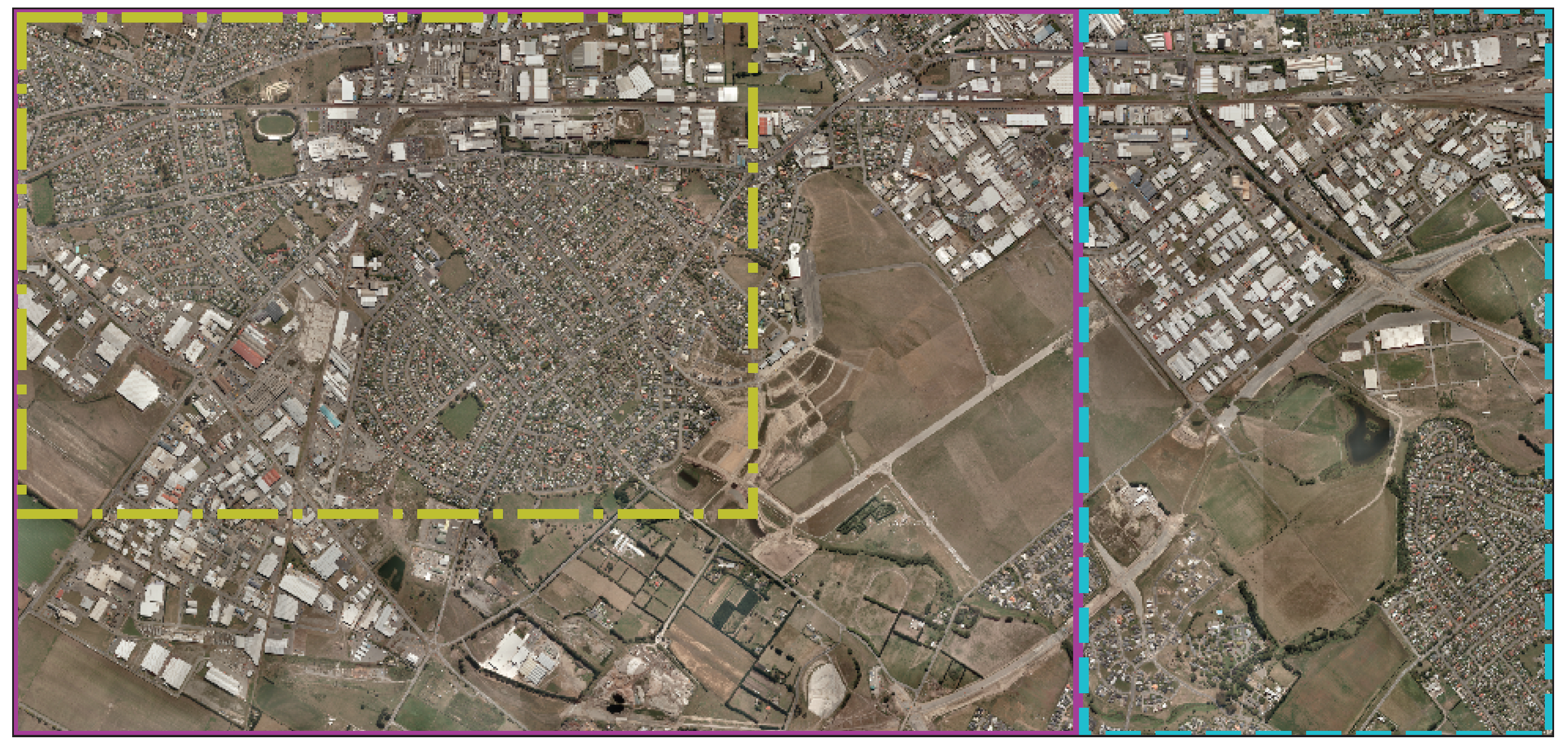
2.6.6. Inference on Large Rasters

Our approach is identical to the one used in [35], with the difference that now we are processing two input images. Interested readers that want to know the full details can refer to Section 3.4 of [35].

During inference on test images, we extract multiple overlapping windows the size of $256\times 256$ with a step (stride) size of $256/4=64$ pixels. The final prediction “probability”, per pixel, is evaluated as the average “probability” over all inference windows that overlap on the given pixel. In this definition, we refer to “probability” as the output of the softmax final classification layer, which is a continuous value in the range $(0,1)$. It is not a true probability in the statistical sense; however, it does express the confidence of the algorithm in obtaining the inference result.

With this overlapping approach, we make sure that the pixels that are closer to the edges and correspond to boundary areas for some inference windows appear closer to the centre area of the subsequent inference windows. For the boundary pixels of the large raster, we apply reflect padding before performing inference [30].

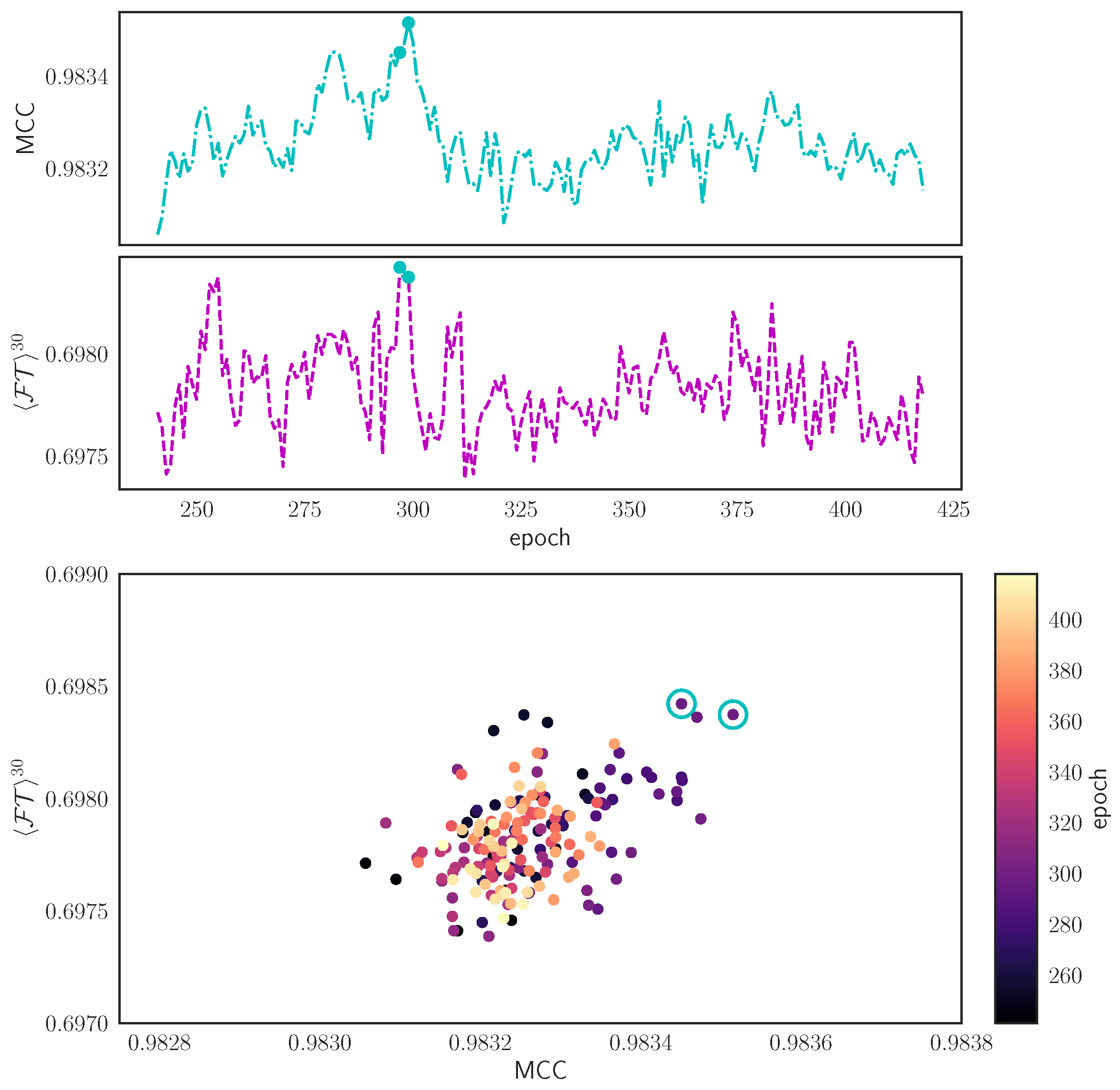
2.6.7. Model Selection Using Pareto Efficiency

For monitoring the performance of our modelling approach, we usually rely on the MCC metric on the validation dataset. We observed, however, that when we perform simultaneously learning rate reduction and ${\langle \mathcal{FT}\rangle }^{\mathfrak{D}}$ depth increase, the MCC initially decreases (indicating performance drop), while the ${\langle \mathcal{FT}\rangle }^{\mathfrak{D}}$ similarity is (initially) strictly increasing. After training starts to stabilise around some optimality region (with the standard noise oscillations), there are various cases where the MCC metric and the ${\langle \mathcal{FT}\rangle }^{\mathfrak{D}}$ similarity coefficient do not agree on which is the best model. To account for this effect and avoid losing good candidate solutions, we evaluate the average of the inference output of a set of the best candidate models. These best candidate models are selected according to the models that belong to the Pareto front of the most-evolved solutions. We use all the Pareto front [54] model’s weights as acceptable solutions for inference. A similar approach was followed for the selection of hyperparameters for optimal solutions in [50].

In Figure 8, we plot, in the top panel, the evolution of the MCC and ${\langle \mathcal{FT}\rangle }^{\mathfrak{D}}$ for $\mathfrak{D}=30$. Clearly, these two performance metrics do not always agree. For example, the ${\langle \mathcal{FT}\rangle }^{30}$ is close to optimality in the approximate epoch ∼250, while the MCC is clearly suboptimal. We highlight the two solutions that belong to the pareto front with filled circles (cyan dots). In the bottom panel, we plot the correspondence of the MCC values with the ${\langle \mathcal{FT}\rangle }^{30}$ similarity metric. The two circles show the corresponding non-dominated Pareto solutions (i.e., best candidates).

3. Results

In this section, we first present an ablation study of the various modules and techniques we introduce. Then, we report the quantitative performance of the models we developed for the task of change detection on the LEVIRCD [1] and WHU [36] datasets. All of the inference visualisations are performed with models having the proposed FracTALdepth $d=5$, although this is not always the best performant network.

3.1. FracTALUnits and Evolving Loss Ablation Study

In this section, we present the performance of the FracTAL ResNet [32,40] and CEECNet units we introduced against ResNet and CBAM [18] baselines as well as the effect of the evolving $L^{\mathfrak{D}}=1-{\langle \mathcal{FT}\rangle }^{\mathfrak{D}}$ loss function on training a neural network. We also present a qualitative and quantitative analysis on the effect of the depth parameter in the FracTALbased on the mantis FracTALResNet network.

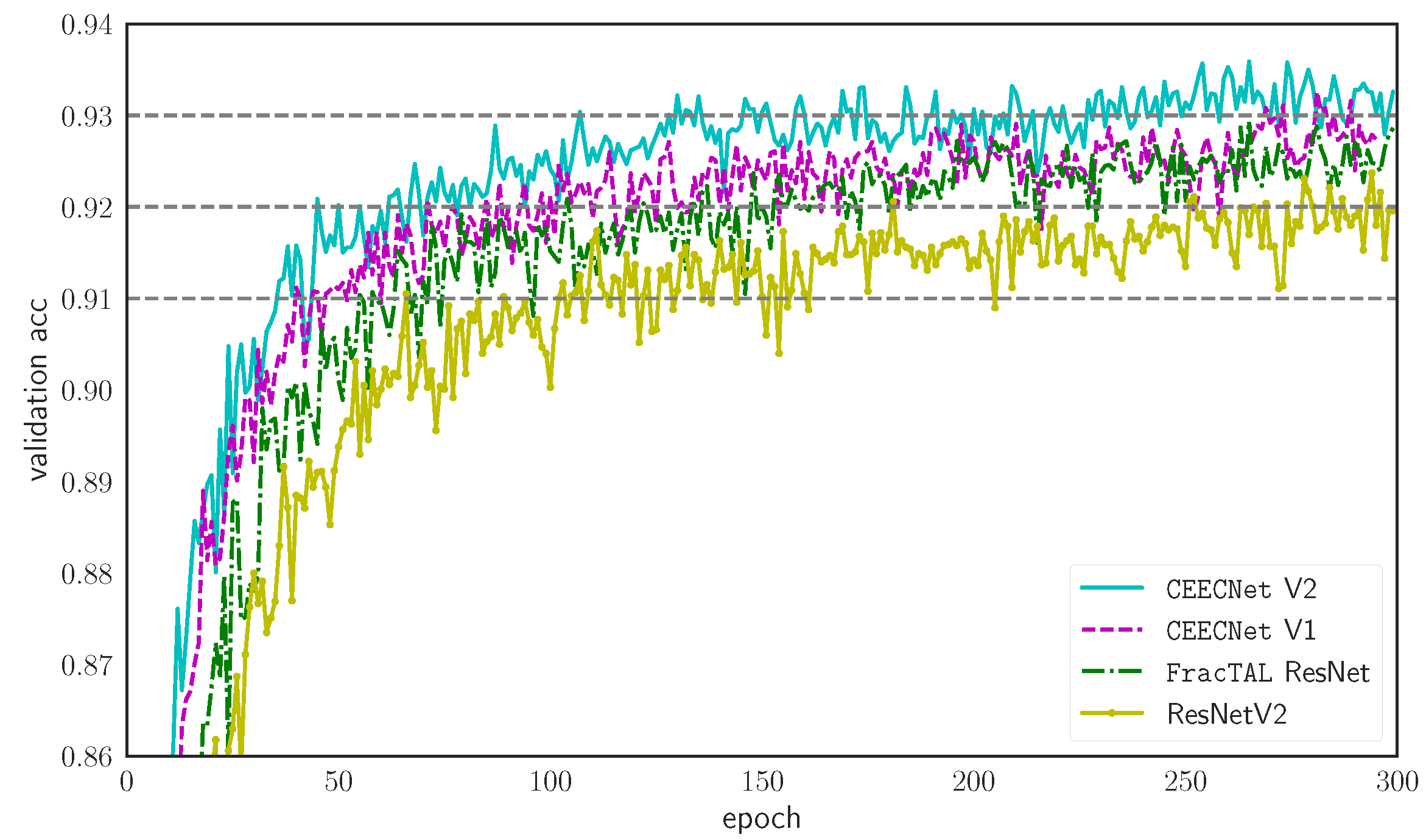
3.1.1. FracTALBuilding Blocks Performance

We construct three identical networks in the macro-topological graph (backbone) but different in micro-topology (building blocks). The first two networks are equipped with two different versions of CEECNet: the first is identical with the one presented in Figure 4b. The second is similar to the one in Figure 4b, with all concatenation operations that are followed by normed convolutions being replaced with Fusion operations, as described in Listing A.3. The third network uses as building blocks the FracTALResNet building blocks (Figure 4a). Finally, the fourth network uses standard residual units as building blocks, as described in [32,40] (ResNet V2). All building blocks have the same dimensionality of input and output features. However, each type of building block has a different number of parameters. By keeping the dimensionality of input and output layers identical to all layers, we believe the performance differences of the networks will reflect the feature expression capabilities of the building blocks we compare.

In Figure 9, we plot the validation loss for 300 epochs of training on CIFAR10 dataset [55] without learning rate reduction. We use cross entropy loss and Adam optimizer [56]. The backbone of each of the networks is described in

Table A1. CEECNetV1 vs. CEECNetV2 vs. FracTALResNet vs. ResNet building blocks comparison. All Building Blocks use kernel size k = 3, padding p = 1 (SAME), and stride s = 1. The transition convolutions that half the size of the features use the same kernel size and padding; however, the stride is s = 2. In the following, we indicate with nf the number of output channels of the convolution layers and with nh the number of heads in the multihead FracTALmodule.

Layers	Proposed Models	ResNet
Layer 1	BBlock[nf = 64, nh = 8]	BBlock[nf = 64]
Layer 2	BBlock[nf = 64, nh = 8 ]	BBlock[nf = 64]
Layer 3	Conv2DN(nf = 128, s = 2)	Conv2DN(nf = 128, s = 2)
Layer 4	BBlock[nf = 128, nh = 16]	BBlock[nf = 128]
Layer 5	BBlock[nf = 128, nh = 16]	BBlock[nf = 128]
Layer 6	Conv2DN(nf = 256, s = 2)	Conv2DN(nf = 256, s = 2)
Layer 7	BBlock[ nf = 256, nh = 32]	BBlock[nf = 256]
Layer 8	BBlock[ nf = 256, nh = 32]	BBlock[nf = 256]
Layer 9	ReLU	ReLU
Layer 10	DenseN(nf = 4096)	DenseN(nf = 4096)
Layer 11	ReLU	ReLU
Layer 12	DenseN(nf = 512)	DenseN(nf = 512)
Layer 13	ReLU	ReLU
Layer 14	DenseN(nf = 10)	DenseN(nf = 10)

. It can be seen that the convergence and performance of all building blocks equipped with the FracTALoutperform standard Residual units. In particular, we find that the performance and convergence properties of the networks follow: ResNet 〈FracTALResNet〈CEECNetV1 〈 CEECNetV2. The performance difference between FracTALResNet and CEECNetV1 will become more clearly apparent in the change detection datasets. The V2 version of CEECNet that uses Fusion with relative attention (cyan solid line) instead of concatenation (V1—magenta dashed line) for combining layers in the Compress-Expand and Expand-Compress branches has superiority over V1. However, it is a computationally more intensive unit.

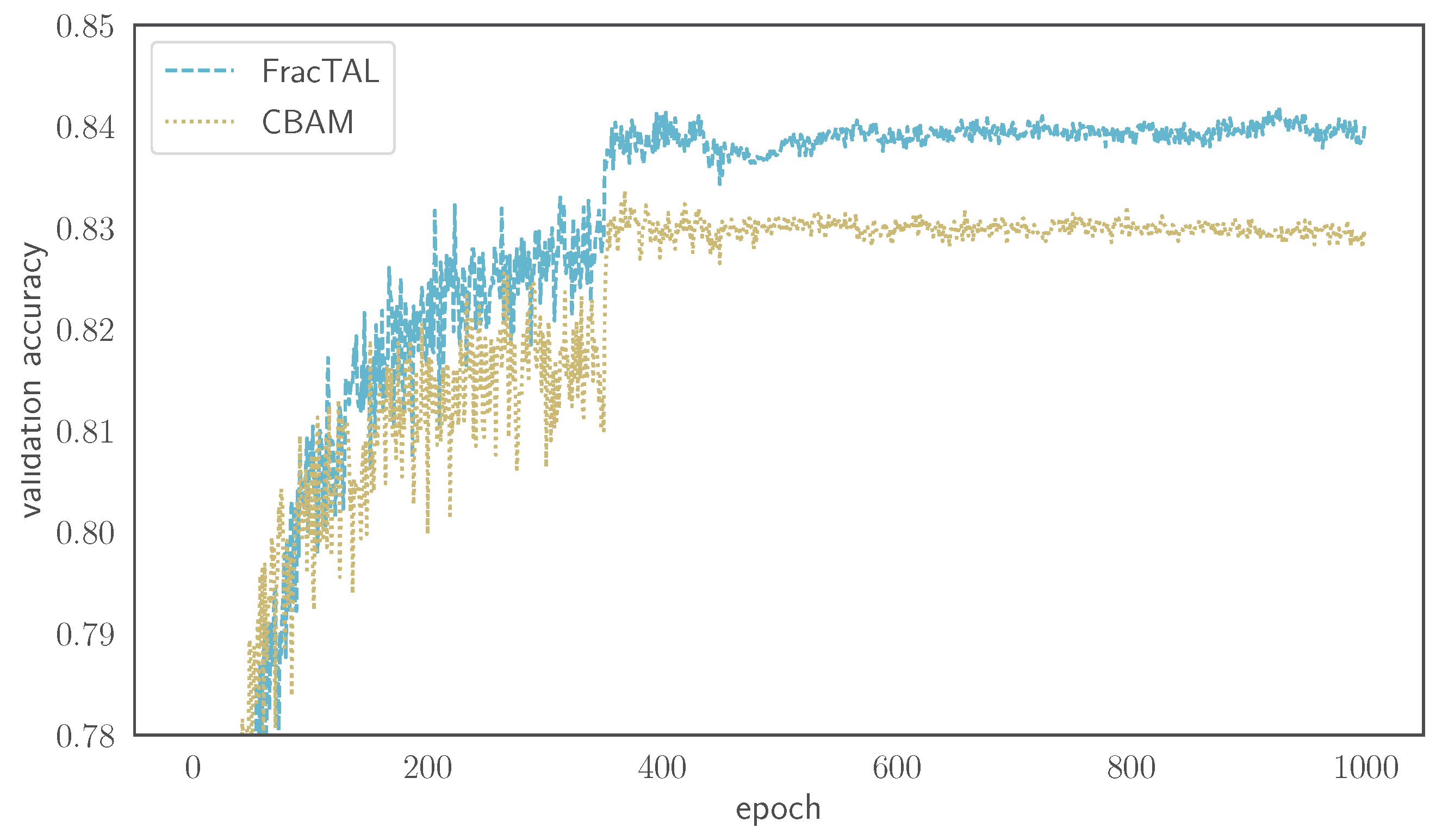
3.1.2. Comparing FracTALwith CBAM

Having shown the performance improvement over the residual unit, we proceed in comparing the FracTALproposed attention with a modern attention module and, in particular, the Convolution Block Attention Module (CBAM) [18]. We construct two networks that are identical in all aspects except the implementation of the attention used. We base our implementation on a publicly available repository that reproduces the results of [18]—written in Pytorch (https://github.com/luuuyi/CBAM.PyTorch, accessed on 1 February 2021)—that we translated into the mxnet framework. From this implementation, we use the CBAM-resnet34 model, and we compare it with a FracTAL-resnet34 model, i.e., a model that is identical to the previous one, with the exception that we replaced the CBAM attention with the FracTAL(attention). Our results can be seen in Figure 10, where a clear performance improvement is evident merely by changing the attention layer used. The improvement is of the order of 1%, from 83.37% (CBAM) to 84.20% (FracTAL), suggesting that the FracTALhas better feature extraction capacity than the CBAM layer.

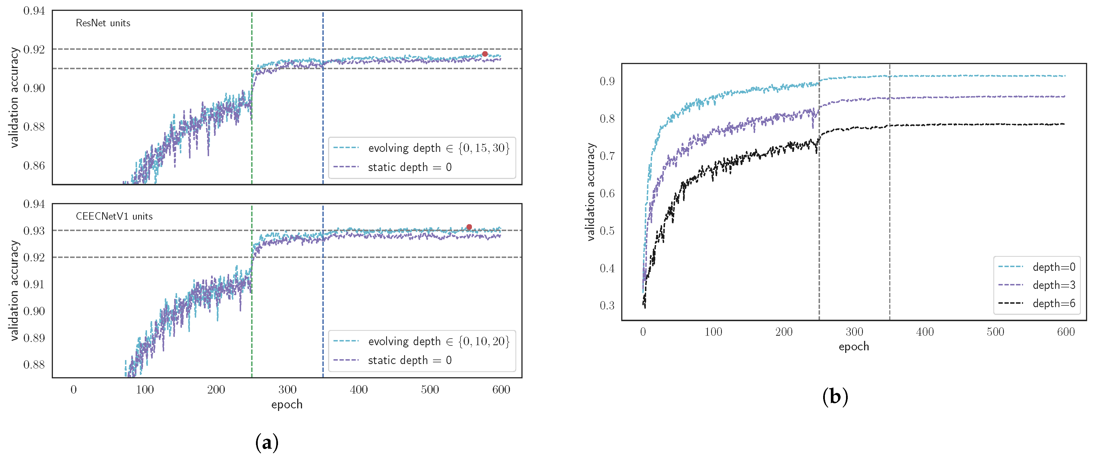
3.1.3. Evolving Loss

We continue by presenting experimental results on the performance of the evolving loss strategy on CIFAR10 using two networks: one with standard ResNet building blocks and one with CEECNetV1 units. The macro-topology of the networks is identical to the one in Table A1. In addition, we also demonstrate performance differences on the change detection task by training the mantis CEECNetV1 model on the LEVIRCD dataset with static and evolving loss strategies for FracTALdepth, $d=5$.

In Figure 11a, we demonstrate the effect of this approach: we train the network on CIFAR10 with standard residual blocks (top panel [32,40]) under the two different loss strategies. In both strategies, we reduce the initial learning rate by a factor of 10 at epochs 250 and 350. In the first strategy, we train the networks with ${\mathcal{FT}}^{\mathfrak{D}=0}$. In the second strategy, we evolve the depth of the fractal Tanimoto loss function: we start by training with ${\mathcal{FT}}^{\mathfrak{D}=0}$, and on the two subsequent learning rate reductions, we use ${\langle \mathcal{FT}\rangle }^{\mathfrak{D}=15}$ and ${\langle \mathcal{FT}\rangle }^{\mathfrak{D}=30}$. In the top panel, we plot the validation accuracy for the two strategies. The performance gain following the evolving depth loss is ∼0.25% in validation accuracy. In the bottom panel, we plot the validation accuracy for the CEECNetV1 -based models. Here, the evolution strategy is same as above with the difference that we use different depths for the $\mathcal{FT}$ loss (to observe potential differences). These are $\mathfrak{D}\in \{0,10,20\}$. Again, the difference in the validation accuracy is $\sim +0.22\%$ for the evolving loss strategy.

We should note that we observed performance degradation by using the $L^{\mathfrak{D}}=1-{\langle \mathcal{FT}\rangle }^{\mathfrak{D}}$loss for $\mathfrak{D}>1$ for training (from random weights). This is evident in Figure 11b where we train from scratch on CIFAR10 three identical models with a different depth for the ${\mathcal{FT}}^{\mathfrak{D}}$ function: $\mathfrak{D}=(0,3,6)$. It is seen that as the hyperparameter $\mathfrak{D}$ increases, the performance of the validation accuracy degrades. We consider that this happens due to the low value of the gradients away from optimality, as it requires the network to train longer to reach the same level of validation accuracy. In contrast, the greatest benefit we observed by using this training strategy is that the network can avoid overfitting after the learning rate reduction (provided that the slope created by the choice of depth $\mathfrak{D}$ is significant) and has the potential to reach higher performance.

Next, we perform a test on evolving vs. static loss strategy on the LEVIR CD change detection dataset, using the CEECNetV1 units, as can be seen in

Table 1. Model comparison on the LEVIR building change detection dataset. We designate with bold font the best values, with underline the second best, and with round brackets, $\left(\right)$ the third best model. All of our frameworks (D6nf32) use the mantis macro-topology and achieve state-of-the-art performance. Here, evo represents evolving loss strategy, sta represents static loss strategy, and the depth d refers to the $\mathcal{FT}$ similarity metric of the FracTAL(attention) layer. In the last column, we provide the number of trainable parameters for each model.

Model	FracTAL Depth	Loss Strategy	Precision	Recall	F1	MCC	IoU	Model Params
Chen and Shi [1]	-	-	83.80	91.00	87.30	-	-	-
CEECNetV1	$d=5$	sta, $\mathfrak{D}\in \{0,10,20,30\}$	93.36	89.46	91.37	90.94	84.10	49.2 M
CEECNetV1	$d=5$	evo, $\mathfrak{D}\in \{0,10,20,30\}$	93.73	(89.93)	(91.79)	(91.38)	(84.82)	49.2 M
CEECNetV2	$d=5$	evo, $\mathfrak{D}\in \{0,10,20,30\}$	93.81	89.92	91.83	91.42	84.89	92.4 M
FracTALResNet	$d=0$	evo, $\mathfrak{D}\in \{0,10,20,30\}$	93.50	89.79	91.61	91.20	84.51	20.1 M
FracTALResNet	$d=5$	evo, $\mathfrak{D}\in \{0,10,20,30\}$	93.60	89.38	91.44	91.02	84.23	20.1 M
FracTALResNet	$d=10$	evo, $\mathfrak{D}\in \{0,10,20,30\}$	(93.63)	90.04	91.80	91.39	84.84	20.1 M

. The CEECNetV1 unit, trained with the evolving loss strategy, demonstrates +0.856% performance increase on the Interesection over Union (IoU) and a +0.484% increase in MCC. Note that, for the same FracTALdepth, $d=5$, the FracTALResNet network trained with the evolving loss strategy performs better than the CEECNetV1 that is trained with the static loss strategy ($\mathfrak{D}=0$), while it falls behind the CEECNetV1 trained with the evolving loss strategy. We should also note that performance increment is larger in comparison to the classification task on CIFAR10, reaching almost ∼1% for the IoU.

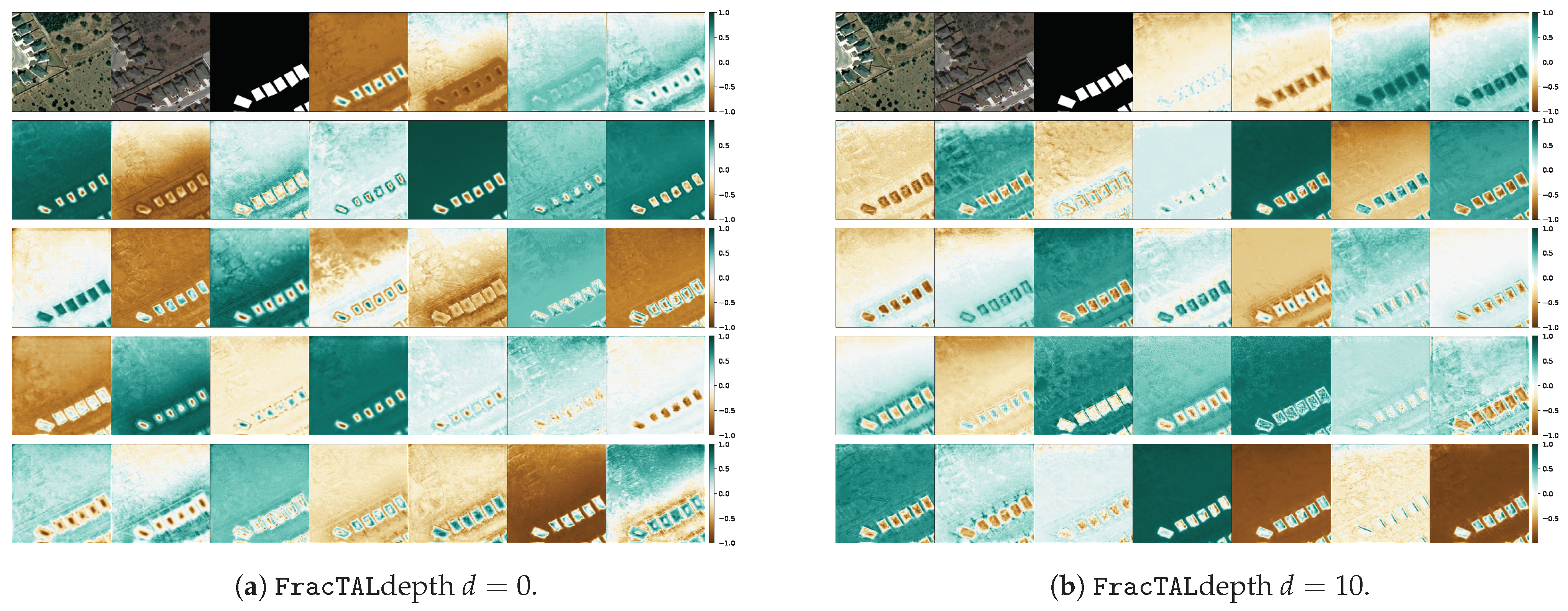
3.1.4. Performance Dependence on FracTALDepth

In order to understand how the FracTALlayer behaves with respect to different depths, we train three identical networks, the mantis FracTALResNet (D6nf32), using FracTALdepths in the range $d\in \{0,5,10\}$. The performance results on the LEVIRCD dataset can be seen in Table 1. It seems the three networks perform similarly (they all achieve SOTA performance on the LEVIRCD dataset), with the $d=10$ having top performance (+0.724% IoU), followed by the $d=0$ (+0.332%IoU), and, lastly, the $d=5$ network (baseline). We conclude that the depth d is a hyperparameter dependent on the problem at task that users of our method can choose to optimise against. Given that all models have competitive performance, it seems that the proposed depth $d=5$ is a sensible choice.

In Figure 12, we visualise the features of the last convolution before the multitasking segmentation head for FracTALdepth $d=0$ (left panel) and $d=10$ (right panel). The features at different depths appear similar, all identifying the regions of interest clearly. To the human eye, according to our opinion, the features for depth $d=10$ appear slightly more refined in comparison to the features corresponding to depth $d=0$ (e.g., by comparing the images in the corresponding bottom rows). The entropy of the features for $d=0$ (entropy: 15.9982) is negligibly higher (+0.00625 %) than for the case $d=10$ (entropy: 15.9972), suggesting both features have the same information content for these two models. We note that, from the perspective of information compression (assuming no loss of information), lower entropy values are favoured over higher values, as they indicate a better compression level.

3.2. Change Detection Performance on LEVIRCD and WHU Datasets

3.2.1. Performance on LEVIRCD

For this particular dataset, a fixed test set is provided, and a comparison with methods that other authors followed is possible. Both FracTAL ResNet and CEECNet (V1, V2) outperform the baseline [1] with respect to the F1 score by ∼5%.

In Figure 13 (see also Figure 1), we present the inference of the CEECNet V1 algorithm for various images from the test set. For each row, from left to right, we have input image at date 1, input image at date 2, ground truth mask, inference (threshold = 0.5), and algorithm’s confidence heat map (this should not be confused with statistical confidence). It is interesting to note that the algorithm has zero doubt in areas where buildings exist in both input images. That is, it is clear our algorithm identifies change in areas covered by buildings and not building footprints. In Table 1, we present numerical performance results of both FracTALResNet as well as CEECNet V1 and V2. All metrics, precision, recall, F1, MCC, and IoU are excellent. The mantis CEECNet for FracTALdepth $d=5$ outperforms the mantis FracTAL ResNet by a small numerical margin; however, the difference is clear. This difference can also be seen in the bottom panel of Figure 16. We should also note that the numerical difference on, say, the F1 score, does not translate to equal portions of quality difference in images. For example, a 1% difference in the F1 score may have a significant impact on the quality of inference. We further discuss this in Section 4.1. Overall, the best model is mantis CEECNet V2 with FracTALdepth $d=5$. Second best is the mantisFracTALResNet with FracTALdepth $d=10$. Among the same set of models (mantisFracTALResNet), it seems that depth $d=10$ performs best; however, we do not know if this generalises to all models and datasets. We consider that FracTALdepth d is a hyperparameter that needs to be fine-tuned for optimal performance, and, as we have shown, the choice $d=5$ is a sensible one as in this particular dataset, it provided us with state-of-the-art results.

3.2.2. Performance on WHU

In

Table 2. Model comparison on the WHU building change detection dataset. We designate with bold font the best values, with underline the second best, and with round brackets, $\left(\right)$, the third best model. Ji et al. [28] presented two models for extracting buildings prior to estimating the change mask. These were the Mask-RCNN (in table: M1) and MS-FCN (in table: M2). Our models consume input images of a size of $256\times 256$ pixels. With the exception of [58] that uses the same size, all other results consume inputs of a size of $512\times 512$ pixels.

Model	FracTAL Depth	Loss Strategy	Precision	Recall	F1	MCC	IoU
Ji et al. [28] M1	-	-	93.100	89.200	(91.108)	-	(83.70)
Ji et al. [28] M2	-	-	93.800	87.800	90.700	-	83.00
Chen et al. [31]	-	-	89.2	(90.5)	89.80	-	-
Cao et al. [57]	-	-	(94.00)	79.37	86.07	-	-
Liu et al. [58]	-	-	90.15	89.35	89.75	-	81.40
FracTALResNet	$d=5$	evo, $\mathfrak{D}\in \{0,10,20,30\}$	95.350	90.873	93.058	92.892	87.02
CEECNetV1	$d=5$	evo, $\mathfrak{D}\in \{0,10,20,30\}$	95.571	92.043	93.774	93.616	88.23

, we present the results of training the mantis network with FracTALResNet and CEECNetV1 building blocks. Both of our proposed architectures outperform all other modelling frameworks, although we need to stress that each of the other authors followed a different splitting strategy of the data. However, with our splitting strategy, we used only 32.9% of the total area for training. This is significantly less than the majority of all other methods we report here, and we should anticipate a significant performance degradation in comparison with other methods. In contrast, despite the relatively smaller training set, our method outperforms other approaches. In particular, Ji et al. [28] used 50% of the raster for training and the other half for testing (Figure 10 in their manuscript). In addition, there is no spatial separation between training and test sites, as it exists in our case, and this should work in their advantage. Furthermore, the use of a larger window for training (their extracted chips are of spatial dimension $512\times 512$) increases in principle the performance because it includes more context information. There is a trade-off here though, in that using a larger window size reduces the number of available training chips; therefore, the model sees a smaller number of chips during training. Chen et al. [31] randomly split their training and validation chips. This should improve performance because there is a tight spatial correlation for two extracted chips that are in geospatial proximity. Cao et al. [57] used as a test set ∼20% of the total area of the WHU dataset; however, they do not specify the splitting strategy they followed for the training and validation sets. Finally, Liu et al. [58] used approximately ∼10% of the total area for the reporting test score performance. They also do not mention their splitting strategy.

In Figure 14, we plot a set of examples of inference on the WHU dataset. The correspondence of the images in each row is identical to Figure 13, with the addition that we denote with blue rectangles the locations of changed buildings (true positive predictions) and missed changes from our model (false negative) with red squares. It can be seen that the most difficult areas are the ones that are heavily populated/heavily built up, and the changes are small area buildings. In Figure A1, we plot from left to right, the test area on date 1, the test area on date 2, the ground truth mask, and the confidence heat map of these predictions.

In this table, we could not include [33] that report performance results evaluated only on the changed pixels and not the complete test images. Thus, they are missing out all false positive predictions that can have a dire impact on the performance metrics. They report precision: 97.840, recall: 97.01, F1: 97.29, and IoU: 97.38.

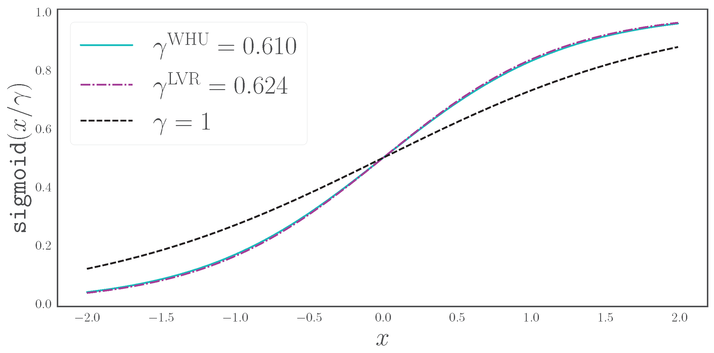
3.3. The Effect of Scaled Sigmoid on the Segmentation HEAD

Starting from an initial value $\gamma =1$ of the scaled sigmoid boundary layer, the fully trained model mantis CEECNetV1 learns the following parameters that control how “crisp” the boundaries should be, or else, how sharp the decision boundary should be:

$$\begin{array}{cc}\hfill {\gamma }_{\mathtt{sigmoid}}^{\mathtt{LVR}}& =0.610\hfill \\ \hfill {\gamma }_{\mathtt{sigmoid}}^{\mathtt{WHU}}& =0.625\hfill \end{array}$$

The deviation of these coefficients from their initial values demonstrates that the network indeed finds it useful to modify the decision boundary. In Figure 15, we plot the standard sigmoid function ($\gamma =1$) and the sigmoid functions recovered after training on the LEVIRCD and WHU datasets.

The algorithm in both cases learns to modify the decision boundary by making it sharper. This means that for two nearby pixels, one belonging to a boundary and the other to a background class, the numerical distance between them needs to be smaller to achieve class separation in comparison with standard sigmoid. Otherwise, a small $\delta x$ change is sufficient to transition between the boundary and no-boundary classes.

4. Discussion

In this section, we comment on the qualitative performance of the models we developed for the task of change detection on the LEVIRCD [1] and WHU [36] datasets. The comparison between CEECNet V1 and FracTALResNet models is for the case of FracTALdepth $d=5$.

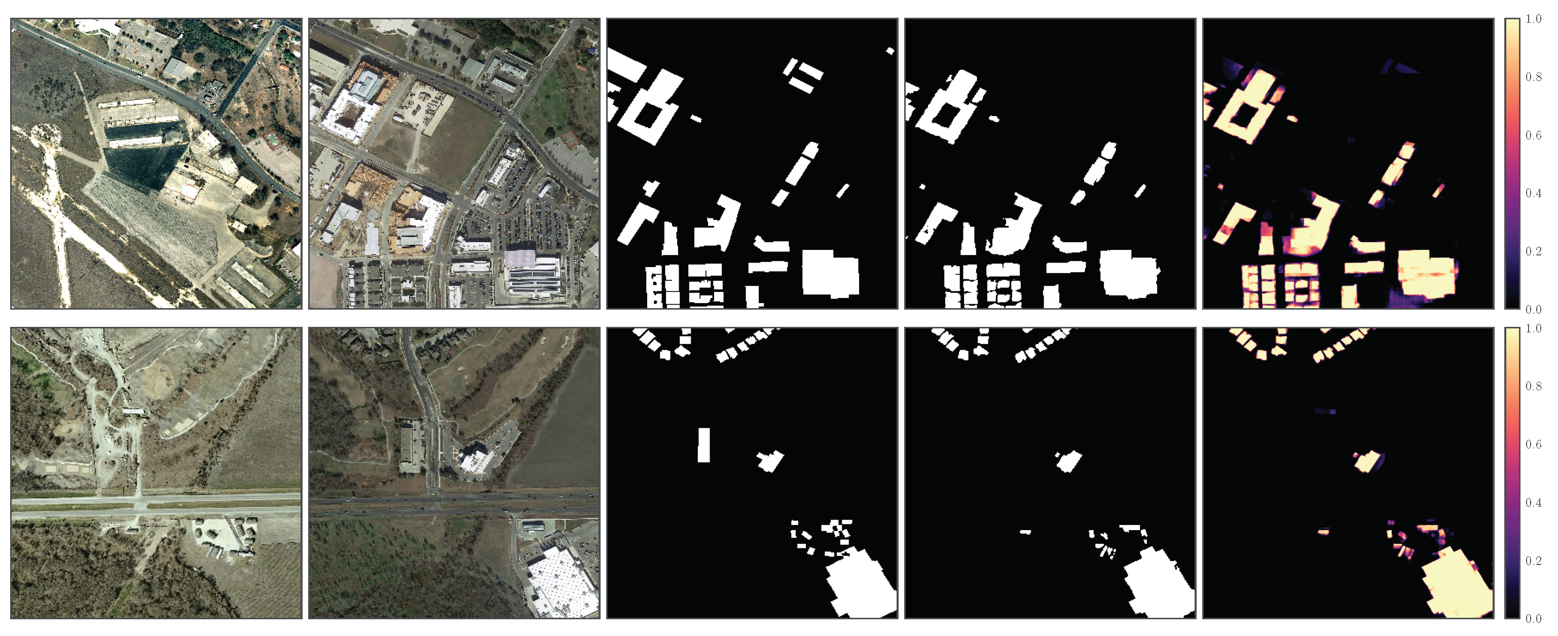
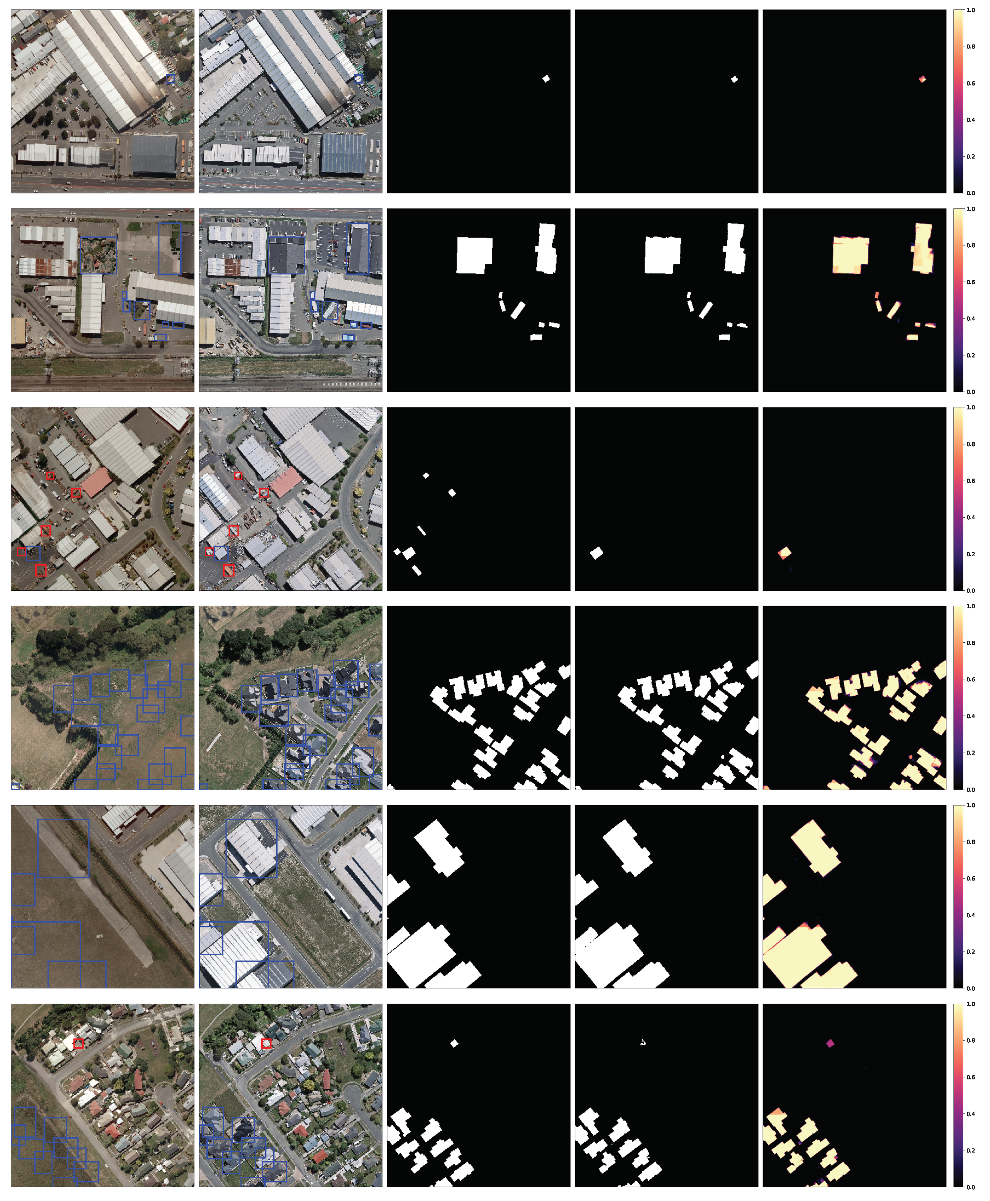
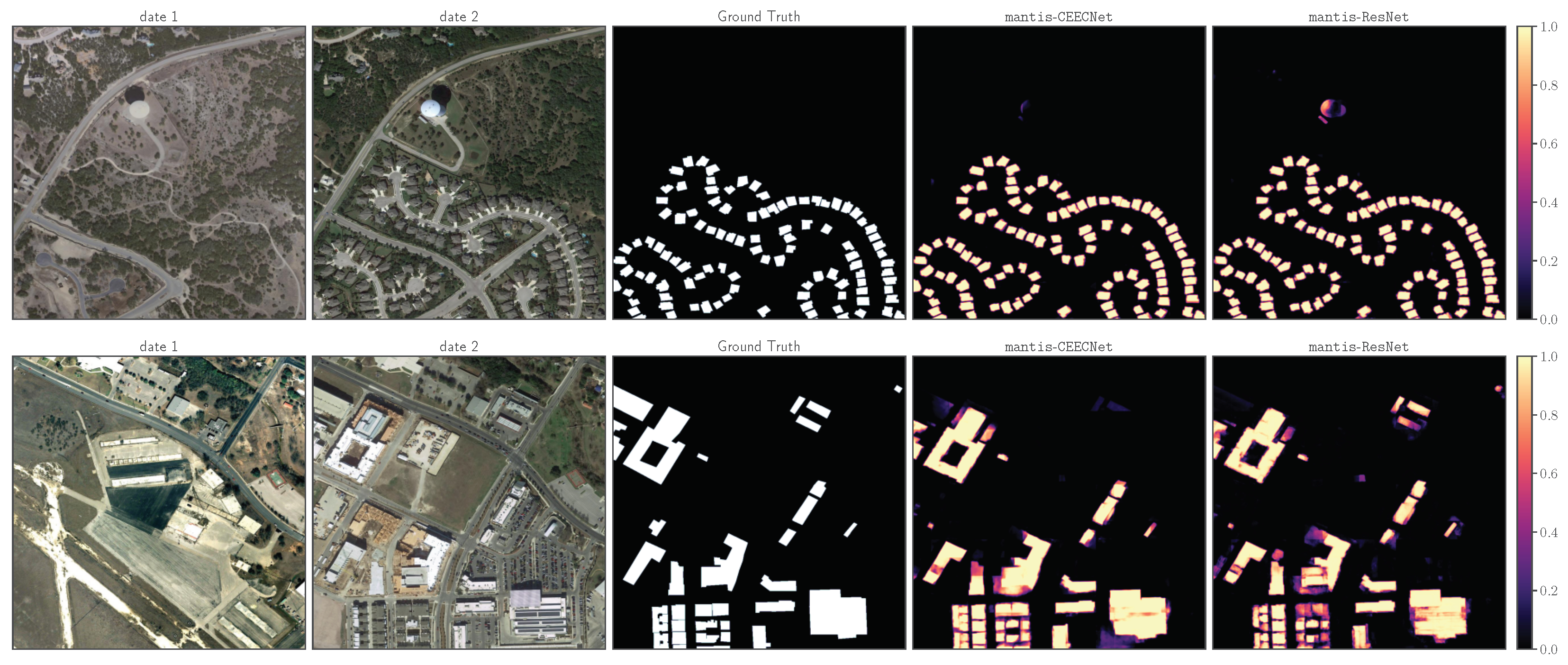
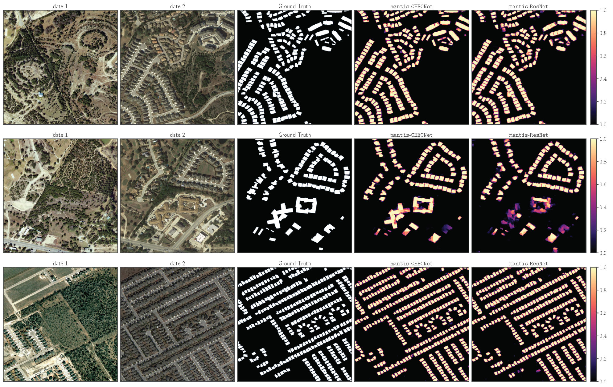
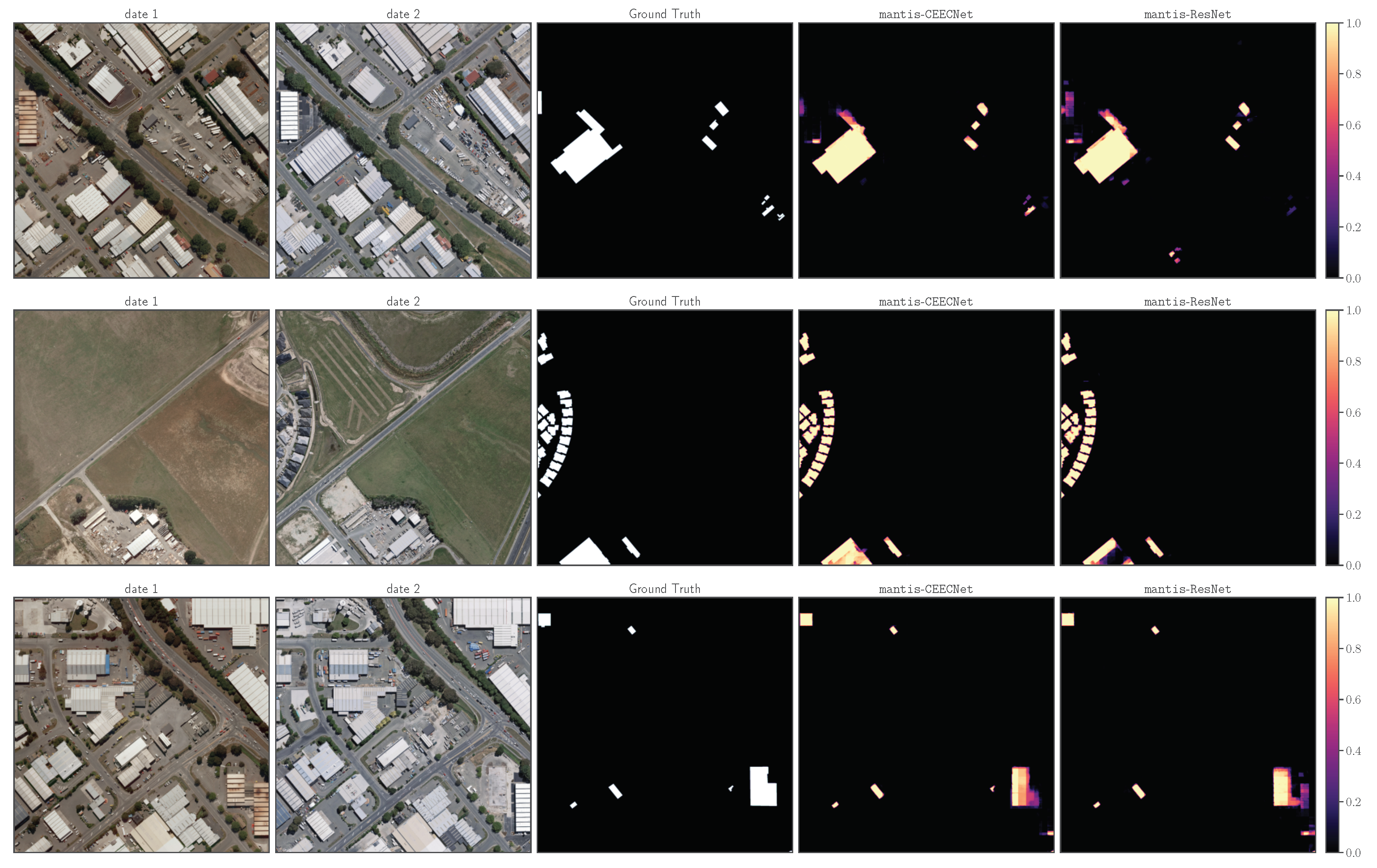
4.1. Qualitative CEECNet and FracTALPerformance

Although both CEECNet V1 and FracTALResNet achieve a very high MCC (Figure 16), the superiority of CEECNet for the same FracTALdepth $d=5$ is evident in the inference maps in both the LEVIRCD (Figure 17) and WHU (Figure 18) datasets. This confirms their relative scores (Table 1 and Table 2) and the faster convergence of CEECNet V1 (Figure 9). Interestingly, CEECNet V1 predicts change with more confidence than FracTALResNet (Figure 17 and Figure 18 ), even when it errs, as can be seen from the corresponding confidence heat maps. The decision on which of the models one should use is a decision to be made with respect to the relative “cost” of training each model, available hardware resources, and the performance target goal.

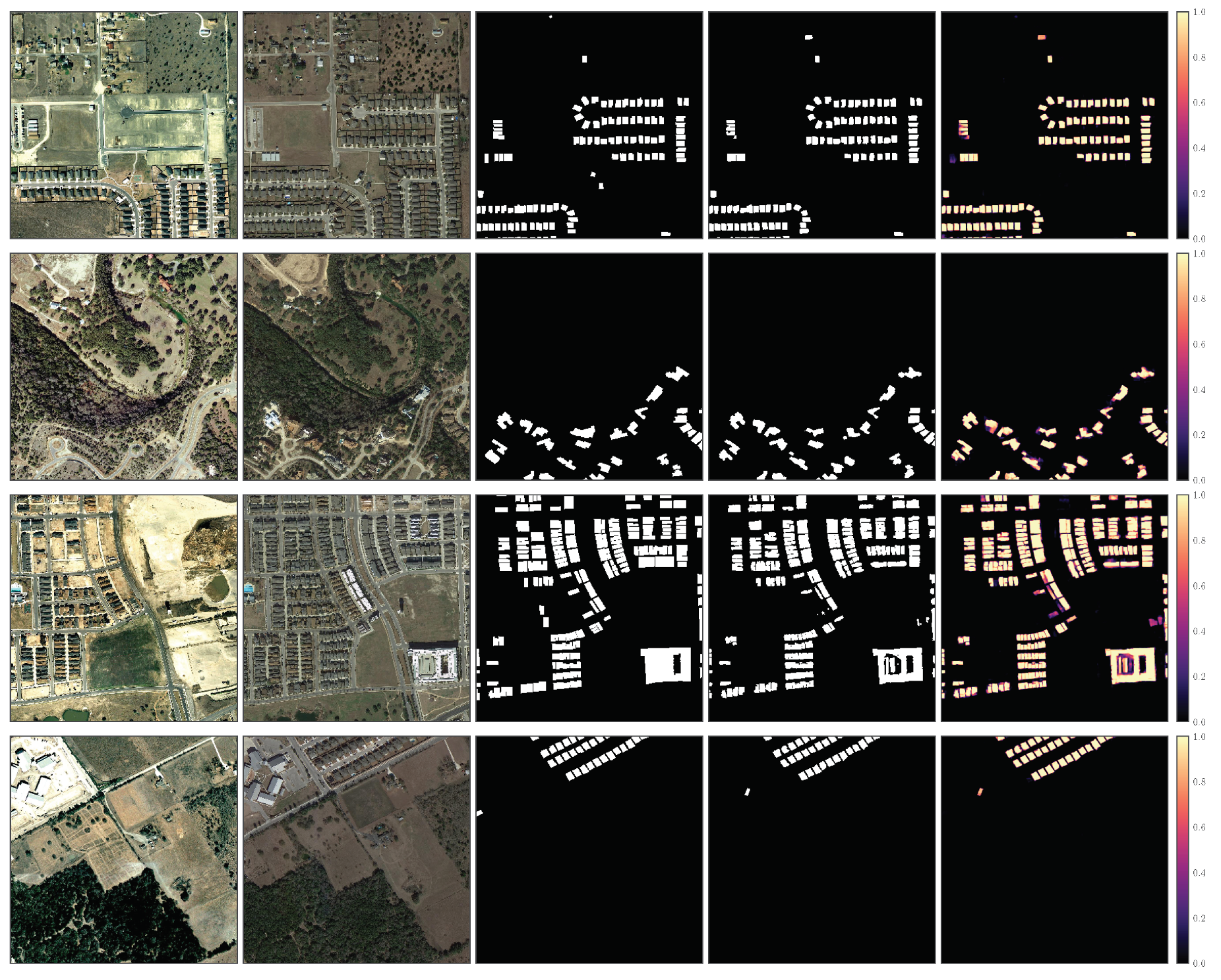
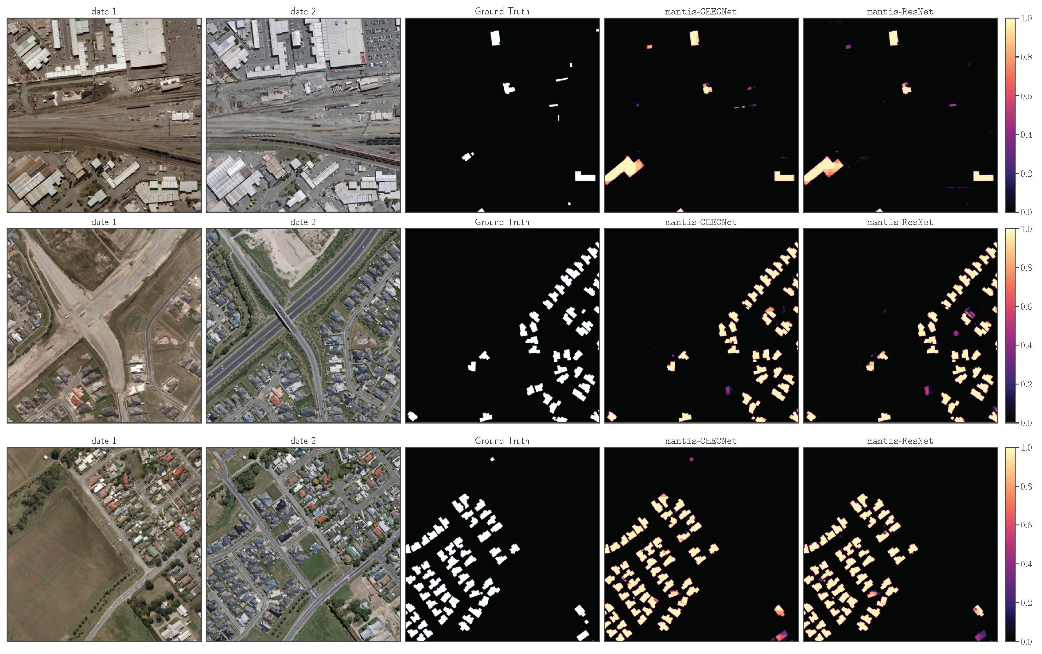
4.2. Qualitative Assesment of the Mantis Macro-Topology

A key ingredient of our approach on the task of change detection is that we emphasise the importance of avoiding using the difference of features to identify changes. Instead, we propose the exchange of information between features extracted from images at different dates with the concept of relative attention (Section 2.5.2) and fusion (Listing A.3). In this section, our aim is to gain insight into the behaviour of the relative attention and fusion layers and compare them with the features obtained by the difference of the outputs of convolution layers of images at different dates. We use the outputs of layers of a trained mantis FracTALResNet model, trained on LEVIRCD with FracTALdepth $d=10$.

In Figure 19, we visualise the features of the first relative attention layers (channels = 32, spatial size $256\times 256$, ratt12 (left panel) and ratt21 (right panel) for a set of image patches belonging to the test set (size: $3\times 256\times 256$). Here, the notation ratt12 indicates that the query features come from the input image at date $t_1$, while the key/value features are extracted from the input image at date $t_2$. Similar notation is applied for the relative attention, ratt21. Starting from the top left corner, we provide the input image at date $t_1$, the input image at date $t_2$, and the ground truth mask of change, and after that, we visualise the features as single channel images. Each feature (i.e., image per channel) is normalised in the range of $(-1,1)$ for visualisation purposes. It can be seen that the algorithm emphasises from the early stages (i.e., first layers) to structures containing buildings and boundaries of these. In particular, the ratt12 (left panel) emphasises boundaries of buildings that exist on both images. It also seems to represent all buildings that exist in both images. The ratt21 layer (right panel) seems to emphasise the buildings that exist on date 1 more but not on date 2. In addition, in both relative attention layers, emphasis on roads and pavements is given.

In Figure 20, we visualise the difference of features of the first convolution layers (channels = 32, spatial size $256\times 256$—left panel) and the fused features (right panel) obtained using the relative attention and fusion methodology (Listing A.3). Some key differences between the two is that we observe that there is less variability within channels in the output of the fusion layer in comparison with the difference of features. In order to quantify the information content of the features, we calculated the Shanon entropy of the features for each case, and we found that the fusion features have half the entropy (11.027) in comparison with the entropy of the difference features (20.97). A similar entropy ratio was found for all images belonging to the test set. This means that the fusion features are less “surprising” than the difference features. This may suggest that the fusion provides a better compression of information in comparison with the difference of layers, assuming both layers have the same information content. It may also mean that the fusion layers have less information content than the difference features, i.e., they are harmful for the change detection process. However, if this was the case, our approach would fail to achieve state-of-the-art performance on the change detection datasets. Therefore, we conclude that the lower entropy value translates to better encoding of information in comparison with the difference of layers.

5. Conclusions

In this work, we propose a new deep learning framework for the task of semantic change detection on very high-resolution aerial images, presented here for the case of changes in buildings. This framework is built on top of several novel contributions that can be used independently in computer vision tasks. Our contributions are:

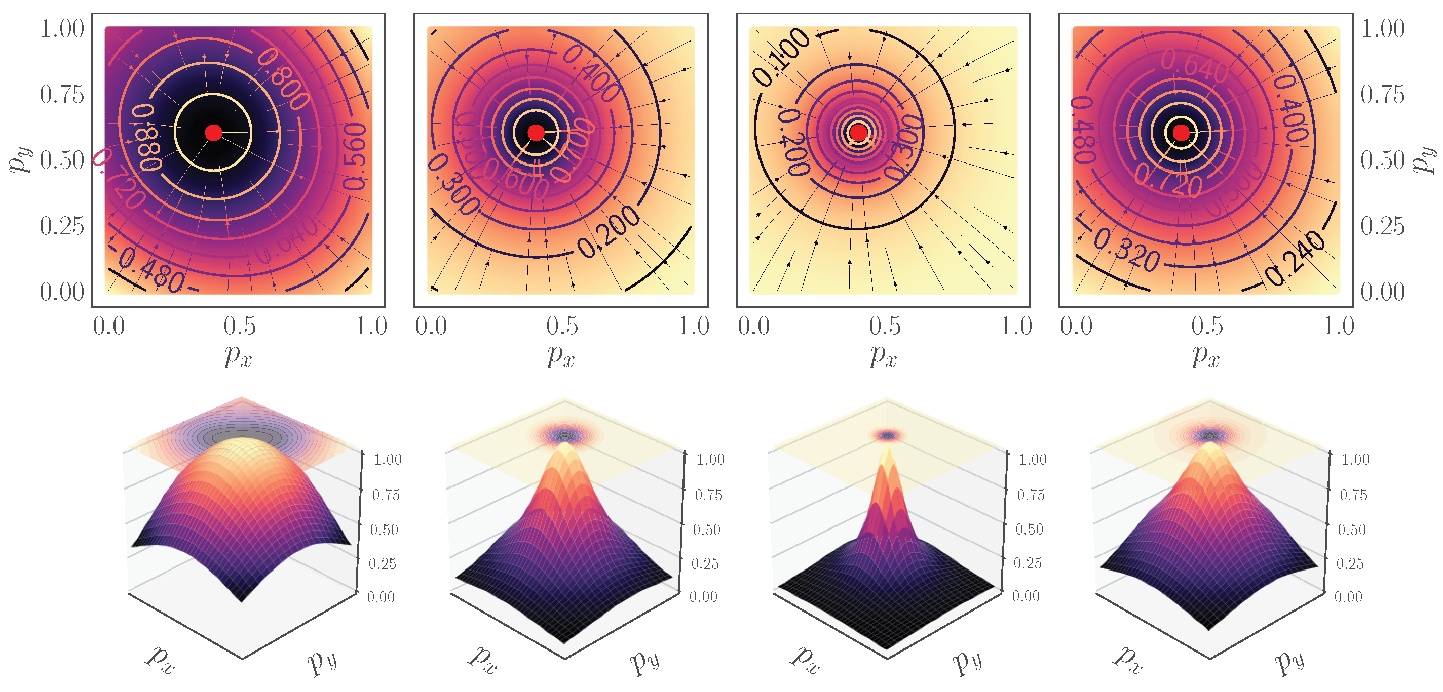
• A novel set similarity coefficient, the fractal Tanimoto coefficient, that is derived from a variant of the Dice coefficient. This coefficient can provide finer detail of similarity at a desired level (up to a delta function), and this is regulated by a temperature-like hyperparameter, d (Figure 2).
• A novel training loss scheme, where we use an evolving loss function, that changes according to learning rate reductions. This helps avoid overfitting and allows for a small increase in performance (Figure 11a,b). In particular, this scheme provided a ∼0.25% performance increase in validation accuracy on CIFAR10 tests, and performance increase of ∼0.9% on IoU and ∼0.5% on MCC on the LEVIRCD dataset.
• A novel spatial and channel attention layer, the fractal Tanimoto Attention Layer (FracTAL—see Listing A.2), that uses the fractal Tanimoto similarity coefficient as a means of quantifying the similarity between query and key entries. This layer is memory efficient and scales well with the size of input features.
• A novel building block, the FracTALResNet (Figure 4a), that has a small memory footprint and excellent convergent and performance properties that outperform standard ResNet building blocks.
• A novel building block, the Compress/Expand–Expand/Compress (CEECNet) unit (Figure 4b), that has better performance than the FracTALResNet (Figure 16), which comes, however, at a higher computational cost.
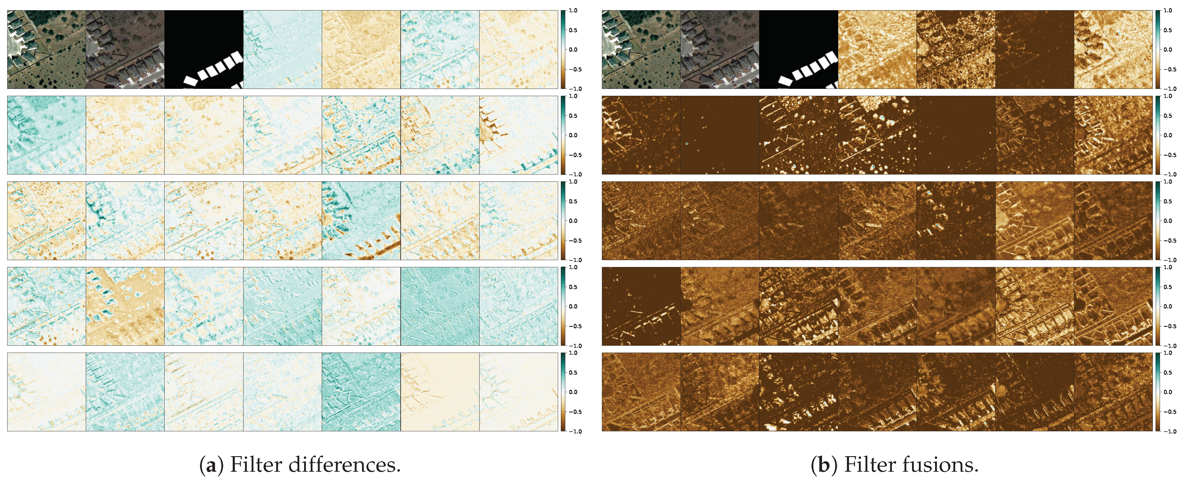
• A corollary that follows from the introduced building blocks is a novel fusion methodology of layers and their corresponding attentions, both for self and relative attention, that improves performance (Figure 16). This methodology can be used as a direct replacement for concatenation in convolution neural networks.
• A novel macro-topology (backbone) architecture, the mantis topology (Figure 5), that combines the building blocks we developed and is able to consume images from two different dates and produce a single change detection layer. It should be noted that the same topology can be used in general segmentation problems, where we have two input images to a network that are somehow correlated and produce a semantic map. Moreover, it can be used for the fusion of features coming from different inputs (e.g., Digital Surface Maps and RGB images).

Altogether, all of the proposed networks that were presented in this contribution, mantis FracTALResNet and mantis CEECNetV1 and V2, outperform other proposed networks and achieve state-of-the-art results on the LEVIRCD [1] and the WHU [36] building change detection datasets (Table 1 and Table 2). Note that there does not exist a standardised test set for the WHU dataset; therefore, relative performance is indicative but not absolute: it depends on the train/test split that other researchers have performed. However, we only used 32.9% of the area of the provided data for training (which is much less than what other methods we compared against have used), and this demonstrated the robustness and generalisation abilities of our algorithm.

In comparison with state-of-the-art architectures that use atrous dilated convolutions, the proposed architectures do not require fine-tuning the dilation rates. Therefore, they are simpler and easier to set up and train.

In this work, we did not experiment with deeper architectures, which would surely improve performance (e.g., D7nf32 models usually perform better), or with hyperparameter tuning. Finally, we should point out that the methods presented here have been successfully applied recently for the task of semantic segmentation (field boundary detection [59]).

References

1. Chen, H.; Shi, Z. A Spatial-Temporal Attention-Based Method and a New Dataset for Remote Sensing Image Change Detection. Remote Sens. 2020, 12, 1662. [Google Scholar] [CrossRef]
2. Giustarini, L.; Hostache, R.; Matgen, P.; Schumann, G.J.P.; Bates, P.D.; Mason, D.C. A change detection approach to flood mapping in urban areas using TerraSAR-X. IEEE Trans. Geosci. Remote Sens. 2012, 51, 2417–2430. [Google Scholar] [CrossRef] [Green Version]
3. Morton, D.C.; DeFries, R.S.; Shimabukuro, Y.E.; Anderson, L.O.; Del Bon Espírito-Santo, F.; Hansen, M.; Carroll, M. Rapid assessment of annual deforestation in the Brazilian Amazon using MODIS data. Earth Interact. 2005, 9, 1–22. [Google Scholar] [CrossRef] [Green Version]
4. Löw, F.; Prishchepov, A.V.; Waldner, F.; Dubovyk, O.; Akramkhanov, A.; Biradar, C.; Lamers, J. Mapping cropland abandonment in the Aral Sea Basin with MODIS time series. Remote Sens. 2018, 10, 159. [Google Scholar] [CrossRef] [Green Version]
5. Caye Daudt, R.; Le Saux, B.; Boulch, A.; Gousseau, Y. Multitask learning for large-scale semantic change detection. Comput. Vis. Image Underst. 2019, 187, 102783. [Google Scholar] [CrossRef] [Green Version]
6. Varghese, A.; Gubbi, J.; Ramaswamy, A.; Balamuralidhar, P. ChangeNet: A Deep Learning Architecture for Visual Change Detection. In Proceedings of the European Conference on Computer Vision (ECCV) Workshops, Munich, Germany, 8–14 September 2018. [Google Scholar]
7. Lu, D.; Mausel, P.; Brondizio, E.; Moran, E. Change detection techniques. Int. J. Remote Sens. 2004, 25, 2365–2401. [Google Scholar] [CrossRef]
8. Coppin, P.; Jonckheere, I.; Nackaerts, K.; Muys, B.; Lambin, E. Review ArticleDigital change detection methods in ecosystem monitoring: A review. Int. J. Remote Sens. 2004, 25, 1565–1596. [Google Scholar] [CrossRef]
9. Tewkesbury, A.P.; Comber, A.J.; Tate, N.J.; Lamb, A.; Fisher, P.F. A critical synthesis of remotely sensed optical image change detection techniques. Remote Sens. Environ. 2015, 160, 1–14. [Google Scholar] [CrossRef] [Green Version]
10. Hussain, M.; Chen, D.; Cheng, A.; Wei, H.; Stanley, D. Change detection from remotely sensed images: From pixel-based to object-based approaches. ISPRS J. Photogramm. Remote Sens. 2013, 80, 91–106. [Google Scholar] [CrossRef]
11. Treisman, A.M.; Gelade, G. A feature-integration theory of attention. Cogn. Psychol. 1980, 12, 97–136. [Google Scholar] [CrossRef]
12. Bahdanau, D.; Cho, K.; Bengio, Y. Neural Machine Translation by Jointly Learning to Align and Translate. arXiv 2014, arXiv:1409.0473. [Google Scholar]
13. Cho, K.; van Merrienboer, B.; Bahdanau, D.; Bengio, Y. On the Properties of Neural Machine Translation: Encoder-Decoder Approaches. arXiv 2014, arXiv:1409.1259. [Google Scholar]
14. Vaswani, A.; Shazeer, N.; Parmar, N.; Uszkoreit, J.; Jones, L.; Gomez, A.N.; Kaiser, L.; Polosukhin, I. Attention Is All You Need. arXiv 2017, arXiv:1706.03762. [Google Scholar]
15. Hu, J.; Shen, L.; Sun, G. Squeeze-and-Excitation Networks. arXiv 2017, arXiv:1709.01507. [Google Scholar]
16. Wang, X.; Girshick, R.B.; Gupta, A.; He, K. Non-local Neural Networks. arXiv 2017, arXiv:1711.07971. [Google Scholar]
17. Chen, L.; Zhang, H.; Xiao, J.; Nie, L.; Shao, J.; Chua, T. SCA-CNN: Spatial and Channel-wise Attention in Convolutional Networks for Image Captioning. arXiv 2016, arXiv:1611.05594. [Google Scholar]
18. Woo, S.; Park, J.; Lee, J.Y.; Kweon, I.S. CBAM: Convolutional Block Attention Module. In Proceedings of the European Conference on Computer Vision (ECCV), Munich, Germany, 8–14 September 2018; Ferrari, V., Hebert, M., Sminchisescu, C., Weiss, Y., Eds.; Springer International Publishing: Cham, Switzerland, 2018; pp. 3–19. [Google Scholar]
19. Bello, I.; Zoph, B.; Vaswani, A.; Shlens, J.; Le, Q.V. Attention Augmented Convolutional Networks. arXiv 2019, arXiv:1904.09925. [Google Scholar]
20. Katharopoulos, A.; Vyas, A.; Pappas, N.; Fleuret, F. Transformers are RNNs: Fast Autoregressive Transformers with Linear Attention. arXiv 2020, arXiv:2006.16236. [Google Scholar]
21. Li, R.; Su, J.; Duan, C.; Zheng, S. Multistage Attention ResU-Net for Semantic Segmentation of Fine-Resolution Remote Sensing Images. arXiv 2020, arXiv:2011.14302. [Google Scholar]
22. Dosovitskiy, A.; Beyer, L.; Kolesnikov, A.; Weissenborn, D.; Zhai, X.; Unterthiner, T.; Dehghani, M.; Minderer, M.; Heigold, G.; Gelly, S.; et al. An Image is Worth 16 × 16 Words: Transformers for Image Recognition at Scale. arXiv 2020, arXiv:2010.11929. [Google Scholar]
23. Sakurada, K.; Okatani, T. Change Detection from a Street Image Pair using CNN Features and Superpixel Segmentation. In Proceedings of the BMVC, Swansea, UK, 7–10 September 2015. [Google Scholar]
24. Alcantarilla, P.F.; Stent, S.; Ros, G.; Arroyo, R.; Gherardi, R. Street-View Change Detection with Deconvolutional Networks. Robot. Sci. Syst. 2016. [Google Scholar] [CrossRef]
25. Guo, E.; Fu, X.; Zhu, J.; Deng, M.; Liu, Y.; Zhu, Q.; Li, H. Learning to Measure Change: Fully Convolutional Siamese Metric Networks for Scene Change Detection. arXiv 2018, arXiv:1810.09111. [Google Scholar]
26. Asokan, A.; Anitha, J. Change detection techniques for remote sensing applications: A survey. Earth Sci. Inform. 2019, 12, 143–160. [Google Scholar] [CrossRef]
27. Shi, W.; Zhang, M.; Zhang, R.; Chen, S.; Zhan, Z. Change Detection Based on Artificial Intelligence: State-of-the-Art and Challenges. Remote Sens. 2020, 12, 1688. [Google Scholar] [CrossRef]
28. Ji, S.; Shen, Y.; Lu, M.; Zhang, Y. Building Instance Change Detection from Large-Scale Aerial Images using Convolutional Neural Networks and Simulated Samples. Remote Sens. 2019, 11, 1343. [Google Scholar] [CrossRef] [Green Version]
29. He, K.; Gkioxari, G.; Dollár, P.; Girshick, R.B. Mask R-CNN. arXiv 2017, arXiv:1703.06870. [Google Scholar]
30. Ronneberger, O.; Fischer, P.; Brox, T. U-Net: Convolutional Networks for Biomedical Image Segmentation. arXiv 2015, arXiv:1505.04597. [Google Scholar]
31. Chen, J.; Yuan, Z.; Peng, J.; Chen, L.; Huang, H.; Zhu, J.; Liu, Y.; Li, H. DASNet: Dual Attentive Fully Convolutional Siamese Networks for Change Detection in High-Resolution Satellite Images. IEEE J. Sel. Top. Appl. Earth Obs. Remote Sens. 2021, 14, 1194–1206. [Google Scholar] [CrossRef]
32. He, K.; Zhang, X.; Ren, S.; Sun, J. Deep Residual Learning for Image Recognition. arXiv 2015, arXiv:1512.03385. [Google Scholar]
33. Jiang, H.; Hu, X.; Li, K.; Zhang, J.; Gong, J.; Zhang, M. PGA-SiamNet: Pyramid Feature-Based Attention-Guided Siamese Network for Remote Sensing Orthoimagery Building Change Detection. Remote Sens. 2020, 12, 484. [Google Scholar] [CrossRef] [Green Version]
34. Lu, X.; Wang, W.; Ma, C.; Shen, J.; Shao, L.; Porikli, F. See More, Know More: Unsupervised Video Object Segmentation with Co-Attention Siamese Networks. In Proceedings of the IEEE Conference on Computer Vision and Pattern Recognition (CVPR), Long Beach, CA, USA, 16–20 June 2019. [Google Scholar]
35. Diakogiannis, F.I.; Waldner, F.; Caccetta, P.; Wu, C. ResUNet-a: A deep learning framework for semantic segmentation of remotely sensed data. ISPRS J. Photogramm. Remote Sens. 2020, 162, 94–114. [Google Scholar] [CrossRef] [Green Version]
36. Ji, S.; Wei, S.; Lu, M. Fully Convolutional Networks for Multisource Building Extraction From an Open Aerial and Satellite Imagery Data Set. IEEE Trans. Geosci. Remote Sens. 2019, 57, 574–586. [Google Scholar] [CrossRef]
37. Zhang, A.; Lipton, Z.C.; Li, M.; Smola, A.J. Dive into Deep Learning. 2020. Available online: https://d2l.ai (accessed on 1 January 2021).
38. Kim, Y.; Denton, C.; Hoang, L.; Rush, A.M. Structured Attention Networks. arXiv 2017, arXiv:1702.00887. [Google Scholar]
39. Zhang, H.; Goodfellow, I.; Metaxas, D.; Odena, A. Self-Attention Generative Adversarial Networks. arXiv 2018, arXiv:1805.08318. [Google Scholar]
40. He, K.; Zhang, X.; Ren, S.; Sun, J. Identity Mappings in Deep Residual Networks. arXiv 2016, arXiv:1603.05027. [Google Scholar]
41. Ioffe, S.; Szegedy, C. Batch Normalization: Accelerating Deep Network Training by Reducing Internal Covariate Shift. arXiv 2015, arXiv:1502.03167. [Google Scholar]
42. Newell, A.; Yang, K.; Deng, J. Stacked Hourglass Networks for Human Pose Estimation. arXiv 2016, arXiv:1603.06937. [Google Scholar]
43. Liu, J.; Wang, S.; Hou, X.; Song, W. A deep residual learning serial segmentation network for extracting buildings from remote sensing imagery. Int. J. Remote Sens. 2020, 41, 5573–5587. [Google Scholar] [CrossRef]
44. Qin, X.; Zhang, Z.; Huang, C.; Dehghan, M.; Zaiane, O.R.; Jagersand, M. U2-Net: Going deeper with nested U-structure for salient object detection. Pattern Recognit. 2020, 106, 107404. [Google Scholar] [CrossRef]
45. Lindeberg, T. Scale-Space Theory in Computer Vision; Kluwer Academic Publishers: Norwell, MA, USA, 1994; ISBN 978-0-7923-9418-1. [Google Scholar]
46. Wang, Z.; Chen, J.; Hoi, S.C.H. Deep Learning for Image Super-resolution: A Survey. arXiv 2019, arXiv:1902.06068. [Google Scholar] [CrossRef] [Green Version]
47. Tschannen, M.; Bachem, O.; Lucic, M. Recent Advances in Autoencoder-Based Representation Learning. arXiv 2018, arXiv:1812.05069. [Google Scholar]
48. Kingma, D.P.; Welling, M. An Introduction to Variational Autoencoders. arXiv 2019, arXiv:1906.02691. [Google Scholar]
49. Zhao, H.; Shi, J.; Qi, X.; Wang, X.; Jia, J. Pyramid Scene Parsing Network. In Proceedings of the CVPR, Honolulu, HI, USA, 21–26 July 2017. [Google Scholar]
50. Waldner, F.; Diakogiannis, F.I. Deep learning on edge: Extracting field boundaries from satellite images with a convolutional neural network. Remote Sens. Environ. 2020, 245, 111741. [Google Scholar] [CrossRef]
51. Wu, Y.; He, K. Group Normalization. arXiv 2018, arXiv:1803.08494. [Google Scholar]
52. Haghighi, S.; Jasemi, M.; Hessabi, S.; Zolanvari, A. PyCM: Multiclass confusion matrix library in Python. J. Open Source Softw. 2018, 3, 729. [Google Scholar] [CrossRef] [Green Version]
53. Matthews, B. Comparison of the predicted and observed secondary structure of T4 phage lysozyme. Biochim. Biophys. Acta (BBA) Protein Struct. 1975, 405, 442–451. [Google Scholar] [CrossRef]
54. Emmerich, M.T.; Deutz, A.H. A Tutorial on Multiobjective Optimization: Fundamentals and Evolutionary Methods. Nat. Comput. Int. J. 2018, 17, 585–609. [Google Scholar] [CrossRef] [Green Version]
55. Krizhevsky, A. Learning Multiple Layers of Features from Tiny Images; Technical Report; Citeseer: Princeton, NJ, USA, 2009. [Google Scholar]
56. Kingma, D.P.; Ba, J. Adam: A Method for Stochastic Optimization. arXiv 2014, arXiv:1412.6980. [Google Scholar]
57. Cao, Z.; Wu, M.; Yan, R.; Zhang, F.; Wan, X. Detection of Small Changed Regions in Remote Sensing Imagery Using Convolutional Neural Network. IOP Conf. Ser. Earth Environ. Sci. 2020, 502, 012017. [Google Scholar] [CrossRef]
58. Liu, Y.; Pang, C.; Zhan, Z.; Zhang, X.; Yang, X. Building Change Detection for Remote Sensing Images Using a Dual Task Constrained Deep Siamese Convolutional Network Model. arXiv 2019, arXiv:1909.07726. [Google Scholar]
59. Waldner, F.; Diakogiannis, F.I.; Batchelor, K.; Ciccotosto-Camp, M.; Cooper-Williams, E.; Herrmann, C.; Mata, G.; Toovey, A. Detect, Consolidate, Delineate: Scalable Mapping of Field Boundaries Using Satellite Images. Remote Sens. 2021, 13, 2197. [Google Scholar] [CrossRef]
60. Chen, T.; Li, M.; Li, Y.; Lin, M.; Wang, N.; Wang, M.; Xiao, T.; Xu, B.; Zhang, C.; Zhang, Z. Mxnet: A flexible and efficient machine learning library for heterogeneous distributed systems. arXiv 2015, arXiv:1512.01274. [Google Scholar]
61. Sergeev, A.; Balso, M.D. Horovod: Fast and easy distributed deep learning in TensorFlow. arXiv 2018, arXiv:1802.05799. [Google Scholar]
Figure 1. Example of the proposed framework change detection performance on the LEVIRCD test set [1] (architecture: mantis CEECNetV1). From left to right: input image at date 1, input image at date 2, ground truth buildings change mask, and colour-coded the true negative (tn), true positive (tp), false positive (fp), and false negative (fn) predictions.
Remotesensing 13 03707 g001
Figure 2. Fractal Tanimoto similarity measure. In the top row, we plot the two-dimensional density maps for the FT similarity coefficient. From left to right, the depths are d { 0 , 3 , 5 } . The last column corresponds to the average of values up to depth d = 5 , i.e., FT 5 = ( 1 / 5 ) d FT d . In the bottom figure, we represent the same values in 3D. The horizontal contour plot at z = 1 corresponds to the Laplacian of the FT . It is observed that as the depth, d, of the iteration increases, the function becomes steeper towards optimality.
Remotesensing 13 03707 g002
Figure 3. Fractal Tanimoto similarity measure with noise. On the top row, from left to right, is the FT 0 ( p , l ) , and ( 1 / 10 ) i = 0 9 ( FT i ( p , l ) ) . The bottom row is the same corresponding FT d ( p , l ) similarity measures with Gaussian random noise added. When the algorithmic training approaches optimality with the standard Tanimoto, local noise gradients tend to dominate over the background average gradient. Increasing the slope of the background gradient at later stages of training is a remedy to this problem.
Remotesensing 13 03707 g003
Figure 4. Left panel (a): the FracTALResidual unit. This building block demonstrates the fusion of the residual block with the self attention layer FracTALevaluated from the input features. Right panel (b): the CEECNet (Compress–Expand/Expand–Compress) feature extraction units. The symbol ⊎ represents concatenation of features along the channel dimension (for V1). For version V2, we replace all of the concatenation operations, ⊎, followed by the normalised convolution layer with relative fusion attention layers, as described in Section 2.4.3 (see also Listing A.3).
Remotesensing 13 03707 g004
Figure 5. The mantis CEECNetV1 architecture for the task of change detection. The Fusion operation (FUSE) is described with mxnet/gluon style pseudocode in detail on Listing A.3.
Remotesensing 13 03707 g005
Figure 6. Conditioned multitasking segmentation HEAD. Here, features 1 and 2 are the outputs of the mantis CEECNet features extractor. The symbol ⊎ represents concatenation along the channels dimension. The algorithm first predicts the distance transform of the classes (regression), then re-uses this information to estimate the boundaries, and finally, both of these predictions are re-used for the change prediction layer. Here, Chng Segm stands for the change segmentation layer and mtsk for multitasking predictions.
Remotesensing 13 03707 g006
Figure 7. Train–validation–test split of the WHU dataset. The yellow (dash-dot line) rectangle represents the training data. The area between the magenta (solid line) and the yellow (dash-dot) rectangles represents the validation data. Finally, the cyan rectangle (dashed) is the test data. The reasoning for our split is to include in the validation data both industrial and residential areas and isolate (spatially) the training area from the test area in order to avoid spurious spatial correlation between training/test sites. The train–validation–test ratio split is train : val : test 33 : 37 : 30 .
Remotesensing 13 03707 g007
Figure 8. Pareto front selection after the last reduction in the learning rate. The bottom panel designates with open cyan circles the two points that are equivalent in terms of quality prediction when both MCC and FT are taken into account. The top two panels show the corresponding evolutions of these measures during training. There, the Pareto optimal points are designated with full circle dots (cyan).
Remotesensing 13 03707 g008
Figure 9. Comparison of the V1 and V2 versions of CEECNet building blocks with a FracTALResNet implementation and a standard ResNet V2 building blocks. The models were trained for 300 epochs on CIFAR10 with standard cross entropy loss.
Remotesensing 13 03707 g009
Figure 10. Performance improvement of the FracTAL-resnet34 over CBAM-resnet34: replacing the CBAM attention layers with FracTALones for two otherwise identical networks results in 1% performance improvement.
Remotesensing 13 03707 g010
Figure 11. Experimental results with the evolving loss strategy for the CIFAR10 dataset. Left panel (a): Training of two classification networks with static and evolving loss strategies. The two networks have identical macro-topologies but different micro-topologies. The first network (top) uses standard Residual units for its building blocks, while the second (bottom) uses CEECNetV1 units. The networks are trained with a static FT ( D = 0 ) loss strategy and an evolving one. We increase the depth D of the L D = 1 FT D ( p , l ) loss function with each learning rate reduction. The vertical dashed lines designate epochs where the learning rate was scaled to 1/10th of its original value. The validation accuracy is mildly increased, although there is a clear difference. Right panel (b): Training on CIFAR10 of a network with standard ResNet building blocks and fixed depth, D , of the L D = 1 FT D loss. The vertical dashed lines designate epochs where the learning rate was scaled to 1/10th of its original value. As the depth of iteration, D , increases ( D remains constant for each experiment), the convergence speed of the validation accuracy degrades.
Remotesensing 13 03707 g011
Figure 12. Visualization of the last features (before the multitasking head) for the mantisFracTALResNet models of FracTALdepth d = 0 (left pannel) and d = 10 (right pannel). The features appear similar. For each panel, the top left first three images are the input image at date t 1 , the input image at date t 2 , and the ground truth mask.
Remotesensing 13 03707 g012
Figure 13. Examples of inferred change detection on some test tiles from the LEVIRCD dataset of the mantis CEECNetV1 model (evolving loss strategy, FracTALdepth d = 5 ). For each row, from left to right, input image date 1, input image date 2, ground truth, change prediction (threshold 0.5), and confidence heat map.
Remotesensing 13 03707 g013aRemotesensing 13 03707 g013b
Figure 14. A sample of change detection on windows the size of 1024 × 1024 from the WHU dataset. Inference is with the mantis CEECNetV1 model. The ordering of the inputs, for each row, is as in Figure 13. We indicate with blue boxes successful findings and with red boxes missed changes on buildings.
Remotesensing 13 03707 g014
Figure 15. Trainable scaling parameters, γ , for the sigmoid activation, i.e., sigmoid ( x / γ ) , that are used in the prediction of change mask boundary layers.
Remotesensing 13 03707 g015
Figure 16. mantisCEECNetV1 vs. mantisFracTALResNet(FracTALdepth, d = 5 ) evolution performance on change detection validation datasets. The top panel corresponds to the LEVIRCD dataset. The bottom panel to the WHU dataset. For each network, we followed the evolving loss strategy: there are two learning rate reductions followed by two scaling ups of the FT d loss function. All four training histories avoid overfitting, thanks to making the loss function sharper towards optimality.
Remotesensing 13 03707 g016
Figure 17. Samples of relative quality change detection on test tiles of size 1024 × 1024 from the LEVIRCD dataset. For each row from left to right: input image date 1, input image date 2, ground truth, and confidence heat maps of mantis CEECNetV1 and mantis FracTALResNet, respectively.
Remotesensing 13 03707 g017aRemotesensing 13 03707 g017b
Figure 18. As in Figure 17 for sample windows of size 2048 × 2048 from the WHU dataset.
Remotesensing 13 03707 g018aRemotesensing 13 03707 g018b
Figure 19. Visualization of the relative attention units, ratt12 (left pannel) and ratt21 (right pannel), for the mantis FracTALResNet with FracTALdepth, d = 10 . These come from the first feature extractors (channels = 32, filter spatial size 256 × 256 ). Here, ratt12 is the relative attention where for query we use input at date t 1 , and the key/value filters are created from input at date t 2 . In the top left rows for each panel, we have input image at date t 1 , input image at date t 2 , and ground truth building change labels, followed by the visualisation of each of the 32 channels of the features.
Remotesensing 13 03707 g019
Figure 20. For the same model as in Figure 19, we plot the difference of the first feature extractor blocks (left panel) vs. the first Fusion feature extraction block (right pannel). The entropy of the fusion features is half that of the difference channels. This means there is less “surprise” in the fusion filters in comparison with the difference of filters for the same trained network.
Remotesensing 13 03707 g020