A Novel Generation Method of High Quality Video Image for High Resolution Airborne ViSAR

Abstract

Video synthetic aperture radar (ViSAR) can provide long-time surveillance of a region of interest (ROI), which is one of the hotspot directions in the SAR field. In order to better display ViSAR, a high resolution and high frame rate are needed. Azimuth integration angle and sub-aperture overlapping ratio, which determine the image resolution and frame rate, respectively, are analyzed in depth in this paper. For SAR imaging algorithm, polar format algorithm (PFA) is applied, which not only has high efficiency but is also easier to integrate with autofocus algorithms. Due to sensitivity to motion error, it is very difficult to obtain satisfactory focus quality, especially for SAR systems with a high carrier frequency. The three-step motion compensation (MOCO) proposed in this paper, which combines GPS-based MOCO, map-drift (MD) and phase gradient autofocus (PGA), can effectively compensate for motion error, especially for short wavelengths. In ViSAR, problems such as jitter, non-uniform grey scale and low image signal noise ratio (SNR) between different aspects images also need to be considered, so a ViSAR generation method is proposed to solve the above problems. Finally, the results of ViSAR in THz and Ku band demonstrate the effectiveness and practicability of the proposed method.

1. Introduction

Video SAR (ViSAR) can display sequential SAR images at a certain rate and has the ability of a dynamic monitoring scene. Compared with traditional SAR imaging results (i.e., static images), ViSAR can provide long-time persistent surveillance of ROI at a high frame rate and can obtain the trajectories of ground moving targets [1,2]. In order to better monitor the scene, a high frame rate and high resolution are required. For the given azimuth resolution, frame rate is proportional to carrier frequency. Thus, ViSAR operating at a high carrier frequency, such as Ka band or THz band, can achieve high resolution and high frame rate simultaneously [3,4]. One drawback of the THz ViSAR is the limited detection range due to hardware limitation. Therefore, the THz ViSAR airborne experiment is hardly to be carried out. At present, some institutions such as Jet Propulsion Laboratory (JPL) [5], Pacific Northwest National Laboratory (PNNL) [6] and High Frequency Physics and Radar Research Center (FHR) [7] have successively developed several THz band SAR systems. The working range of the MIRANDA-300 system [8], designed by FHR and operating with a center frequency of 300 GHz, was up to 500 m in 2015.

Spotlight mode is the main mode for ViSAR [9]. The Back-Projection (BP) [10,11,12] and the polar format algorithm (PFA) [4,13,14] are two useful methods for spotlight SAR imaging. Compared with the BP algorithm, PFA is more efficient and easier to integrate with autofocus algorithms like Map-Drift (MD) [15] and phase gradient autofocus (PGA) [16]. Therefore, PFA is widely used in spotlight SAR imaging. However, phase error. introduced by the planar approximation of PFA, causes image distortion and defocusing [17,18,19]. As the scene expands, the distortion and defocusing are more and more severe. Therefore, the depth of focus (DOF) of PFA is limited. The distortion of images can be corrected by the 2D image interpolation that projects the image grids onto an actual position [18]. Some methods, such as spatially variant post filtering (SVPF) [17,20,21] and sub-block imaging [22], are proposed to avoid the defocusing of imaging results.

To achieve high resolution, phase error caused by non-ideal motion must be compensated for, especially in the case of SAR systems with high carrier frequency, because the short wavelength is more sensitive to motion error [23,24,25]. The most common motion compensation (MOCO) method is GPS-based MOCO, which is based on aircraft motion measurement data measured by GPS. This method is simple and efficient, which is more suitable for real-time MOCO. However, GPS-based MOCO depends on a high precision GPS, which increases the cost of experiment, and the GPS accuracy is difficult to achieve centimeter lever. Apart from GPS-based MOCO, some autofocused techniques that are based on echo data have been proposed. One type is parametric, and it employs the polynomial phase error model, e.g., the reflectivity displacement method (RDM) [26] and the MD technique [15,25]. The other type of solution is nonparametric, e.g., the rank one phase estimator (ROPE) [27], shear averaging [28] and PGA [16,25]. The effectiveness of these methods has been demonstrated by experiment data. However, in case of a very fine azimuth resolution, the phase error caused by motion error tends to be of a higher order. Under such conditions, even if the residual range cell migration (RCM) could be compensated for, some autofocused methods still suffer from performance degradation. MD can only estimate quadratic phase error, which cannot compensate for a higher order phase error. PGA can compensate for any higher order phase error, theoretically. Nevertheless, the main lobe widening and energy loss in the presence of a significant high-order phase error affect the performance of PGA [29,30]. In recent years, MOCO based on wavelet transform (WT) has been proposed to correct the vibration error in THz band [31]. Normally, neural network can be used for imaging a high-quality image [32]. With the increasing requirement for resolution, the topography variation, phase unwrapping and two-axis gimbal stabilization still need to be considered [33,34,35].

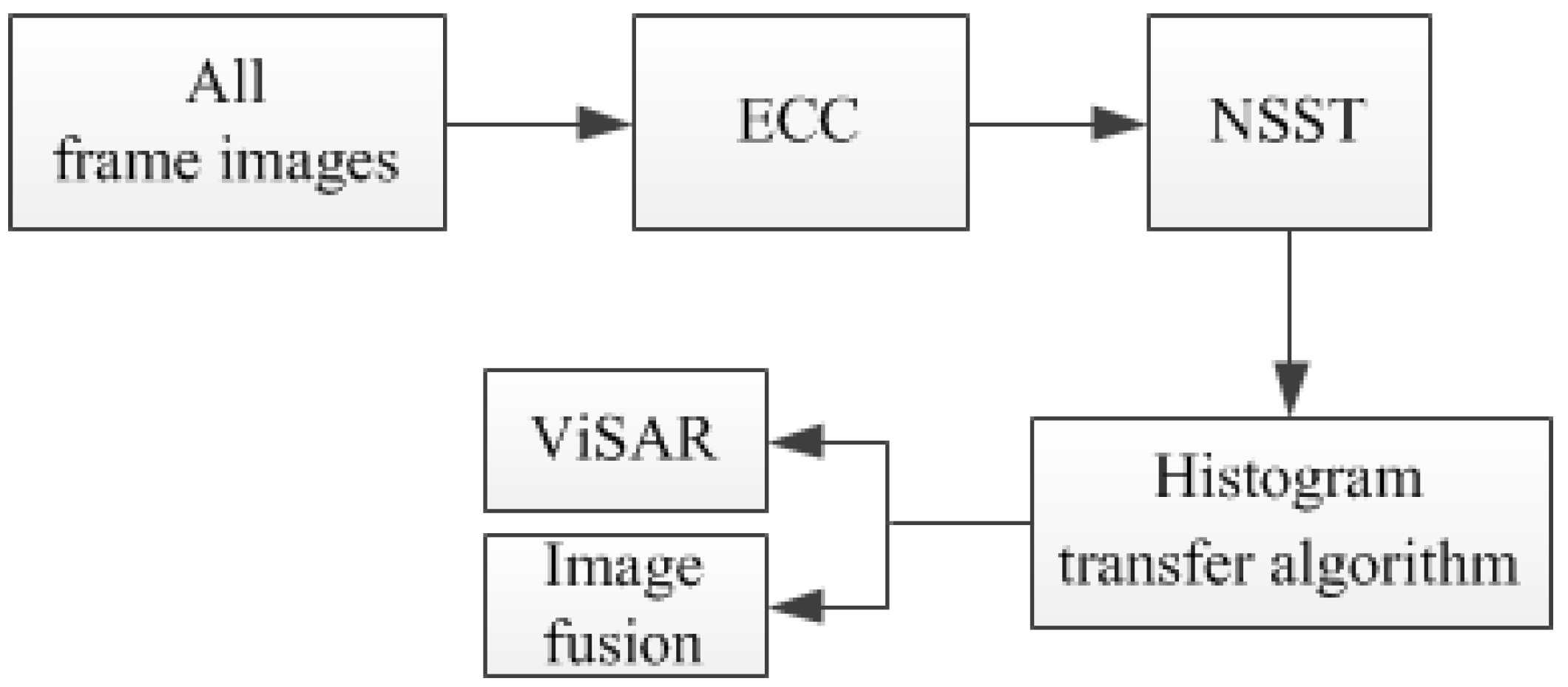
In this paper, we propose the generation method of ViSAR and present the results of airborne ViSAR in THz and Ku band, respectively. First, the PFA for spotlight SAR is described, and the planar approximation of PFA is analyzed. The relationship between the coherent accumulation angle and the azimuth resolution and the relationship between the video frame rate and overlapping ratio are analyzed in depth. Furthermore, considering the difficulty of MOCO for fine azimuth resolution, three-step MOCO, which combines GPS-based MOCO, MD and PGA, is proposed for high resolution imaging. Three-step MOCO, which was refocused by MD before PGA, can improve the performance of PGA. Furthermore, to generate the video result, problems such as the jitter, non-uniform greyscale and low image SNR between images obtained from different aspect angles should be overcome. So, a ViSAR generation method is proposed to solve the above problems. By the proposed method, the satisfactory results of ViSAR in the THz and Ku band are presented in this paper. To the best of our knowledge, this is the first airborne linear spotlight ViSAR result at the THz band. We demonstrate the capability of using extremely short sub-apertures and a low overlapping ratio to generate high resolution and high frame rate ViSAR. The effectiveness of three-step MOCO is also validated. To further verify the efficiency of the generation method of ViSAR with a wide observation scene, another CSAR experiment in Ku band is carried out. What’s more, compared with linear spotlight SAR, circular SAR (CSAR), which illuminates targets from wide aspect angles, has the capability of monitoring urban scenes. For example, according to shadow information of ground moving targets, we can obtain their trajectories.

The main contributions of this paper are

(i).

The three-step MOCO, which was first applied to high resolution imaging, can effectively compensate for motion error;

(ii).

The procedure of ViSAR that is proposed in this paper can effectively improve ViSAR quality;

This paper is organized as follows. Section 2 describes the ViSAR model. In Section 3, procedure of ViSAR is introduced in detail. In Section 4, the results of the experimental data are shown. Finally, the conclusion is given in Section 5.

2. ViSAR Model

2.1. Theory of ViSAR Imaging Algorithm

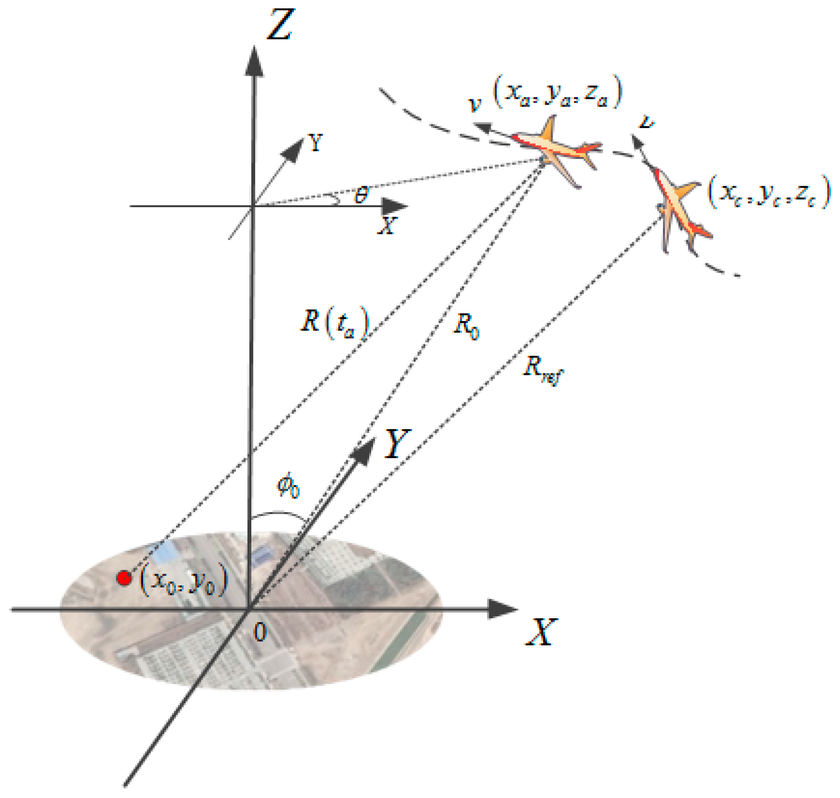
The geometry of airborne spotlight SAR is shown in Figure 1. In Figure 1, the radar antenna is continuously steered to illuminate a fixed scene as the platform flies along an imaginary line with the speed $V$. The echo of target can be described as

$$\begin{array}{l}s\left(t,t_a\right)=A·\mathrm{rect}\left(\frac{t-2·R\left(t_a\right)/c}{T_p}\right)·\\ \begin{array}{cc}\begin{array}{cc}& \end{array}& \end{array} \exp \left(j2\pi \left[f_c\left(t-2·R\left(t_a\right)/c\right)+\frac{1}{2}\gamma {\left(t-2·R\left(t_a\right)/c\right)}^2\right]\right)\end{array}$$

(1)

where $A$ is the amplitude of signal, $T_p$ is the signal time width, $f_c$ is the center frequency, $\gamma$ is the Doppler rate, $c$ is the speed of light, $t$ is the fast-time, $t_a$ is the slow-time. $R\left(t_a\right)$ denotes the instantaneous distance between platform position $\left(x_a,y_a,z_a\right)$ and target $\left(x_0,y_0,0\right)$ and it can be described as

$$R\left(t_a\right)=\sqrt{{\left(x_a-x_0\right)}^2+{\left(y_a-y_0\right)}^2+z_a^2}$$

(2)

Let $R_0$ denote the instantaneous slant range from platform position to scene center

$$R_0=\sqrt{x_a^2+y_a^2+z_a^2}$$

(3)

Scene center is selected as the reference point for MOCO. To simplify the subsequent analysis without loss of generality, the curvilinear aperture is assumed to have occurred in the slow time interval of $t_a\in \left(-1,1\right)$, therefore the time instant at the aperture center is defined as the initial time $\left(t_a=0\right)$. The coordinates of the aperture center are denoted by ${\left(x_c,y_c,z_c\right)=\left(x_a,y_a,z_a\right)|}_{t=0}$ and the slant range $R_{\mathrm{ref}}$ can be expressed as

$$R_{\mathrm{ref}}=\sqrt{x_c^2+y_c^2+z_c^2}$$

(4)

The de-chirp signal can be expressed as

$$\begin{array}{ll}ss\left(t,t_a\right)& =A·\mathrm{rect}\left(\frac{t-2·R/c}{T_p}\right)\exp (-j\frac{4\pi }{c}\gamma \left(t-2·R_{\mathrm{ref}}/c\right)R_{\Delta }\\ & -j\frac{4\pi }{c}{f}_c{R}_{\Delta }+j\frac{4\pi \gamma }{c^2}{R}_{\Delta }^2)\end{array}$$

(5)

where $R_{\Delta }=R-R_{\mathrm{ref}}$. The last term in Equation (5) is the residual video phase (RVP) which should be removed. The expression of Equation (5) in wavenumber domain is

$$Ss\left(k,t_a\right)=A·\mathrm{rect}\left(\frac{k}{2B/c}\right)\exp \left(-j\left(k+k_c\right)R_{\Delta }\right)$$

(6)

In Equation (6), $k=\frac{4\pi }{c}\gamma \left(t-2·R_{\mathrm{ref}}/c\right)$ and $k_c=\frac{4\pi f_c}{c}$. $R_{\Delta }$ can be expressed with Taylor expansion

$$\begin{array}{ll}{R}_{\Delta }& =R-R_{\mathrm{ref}}\\ & =-x_0\sin {\varphi }_0\cos \theta -y_0\sin {\varphi }_0\sin \theta +R_{\mathrm{HOT}}\left(x_0,y_0,\theta \right)\\ & \approx -x_0\sin {\varphi }_0\cos \theta -y_0\sin {\varphi }_0\sin \theta \end{array}$$

(7)

$R_{\mathrm{HOT}}\left(x_0,y_0,\theta \right)$ is the higher order term which is neglected in planar wave approximation [10,13,14]. ${\varphi }_0$ and $\theta$ are depression and corresponding azimuth angles in coordinate system and the expression is

$$\{\begin{array}{l}\theta =\arctan \left(\frac{y_a}{x_a}\right)\\ {\varphi }_0=\arccos \left(\frac{z_a}{R_0}\right)\end{array}$$

(8)

Substituting the expression of Equation (7) into Equation (6) and the expression can be rewritten as

$$Ss\left(k_x,k_y\right)=A·\mathrm{rect}\left(\frac{k}{2B/c}\right)\exp \left(-j{k}_x{x}_0\right)\exp \left(-j{k}_y{y}_0\right)$$

(9)

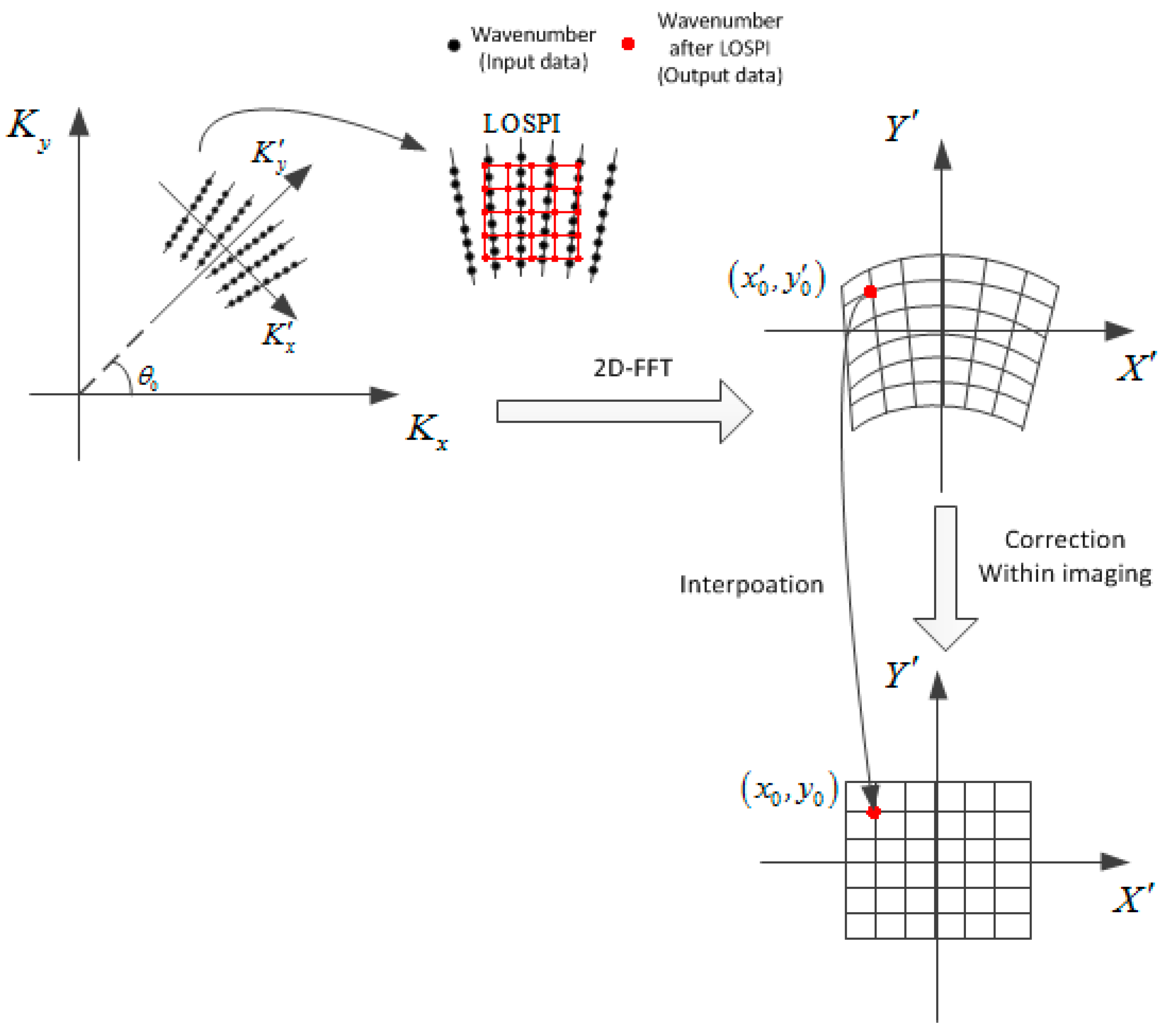
where $k_x=-\left(k+k_c\right)\sin {\varphi }_0\cos \theta$, $k_y=-\left(k+k_c\right)\sin {\varphi }_0\sin \theta$. According to the expression of $k_x$ and $k_y$, the spectrum in wavenumber domain is nonuniform. In order to project the nonuniform result onto a uniform grid in wavenumber domain, the Line-of-Sight Polar Interpolation (LOSPI) is applied [3,10]. The coordinate system is rotated to the direction of Line of Sight (LOS) in LOSPI. After interpolation, applying 2D FFT to obtain desired image

$$I(x,y)={\displaystyle \iint Ss\left(k_x,k_y\right)\exp (-j{k}_{x}x-j{k}_{y}y)d}{k}_{x}d{k}_y$$

(10)

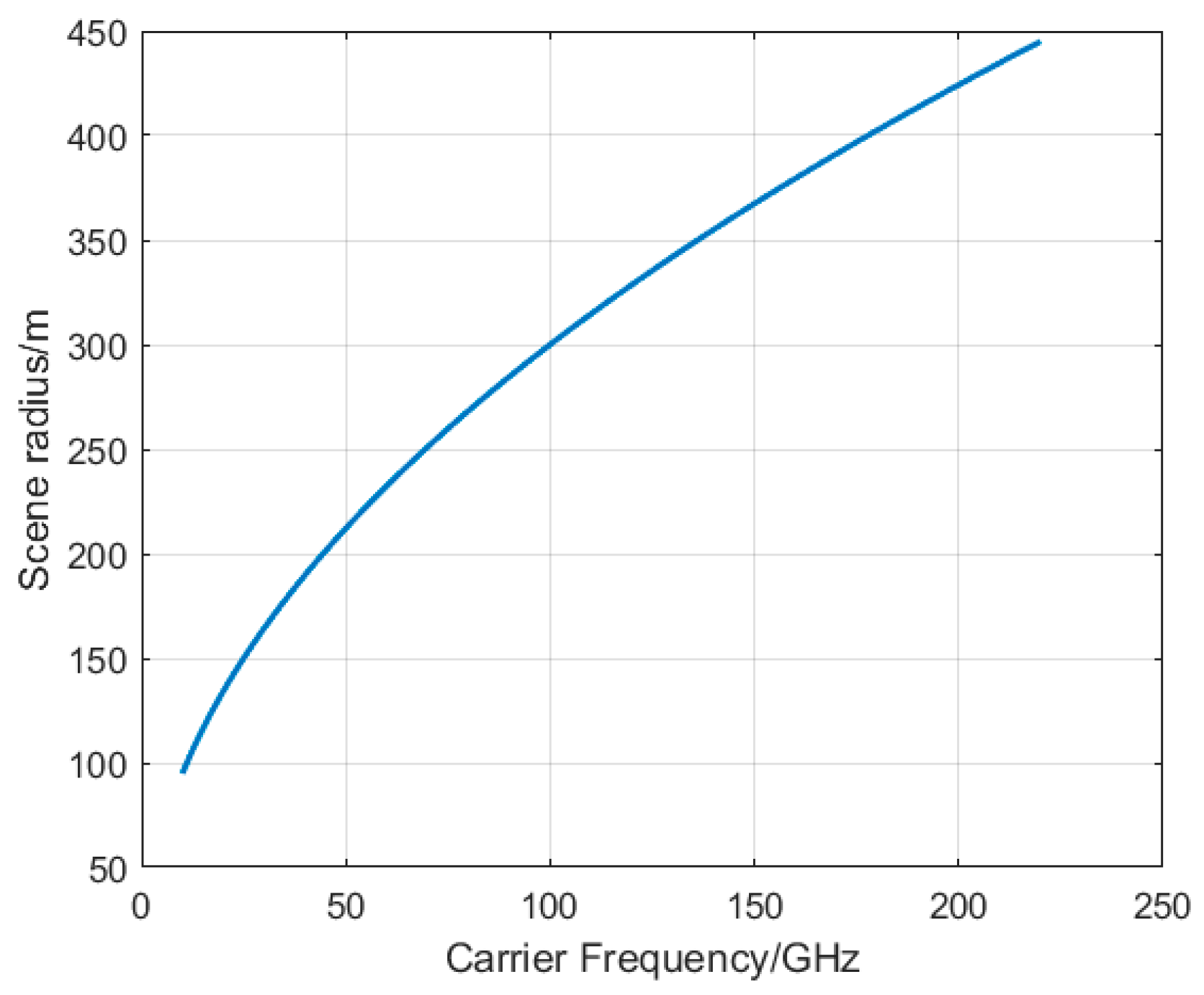
When the imaging scene is large, the $R_{\mathrm{HOT}}\left(x_0,y_0,\theta \right)$ in Equation (7) cannot be eliminated. The phase error caused by $R_{\mathrm{HOT}}\left(x_0,y_0,\theta \right)$ may affect the imaging quality seriously. The primary phase error causes distortion, and the QPE causes defocusing. For an image that is defocused, according to the expression of QPE the expression of the maximal allowable scene radius can be derived [3,10].

$$r=2{\rho }_x\sqrt{\frac{R_{\mathrm{ref}}}{{\lambda }_c}}$$

(11)

where ${\rho }_x$ is azimuth resolution, ${\lambda }_c$ is wavelength, $r$ is the maximal allowable scene radius. For given azimuth resolution 0.15 m, the relationship between scene radius and carrier frequency is shown in Figure 2.

From Figure 2, with the higher carrier frequency, the maximal allowable scene radius is longer. For allowable region that is larger than ROI, the QPE of the traditional PFA images can be neglected and all the targets in the whole ROI have a good, focused performance. If ROI is larger than the allowable region, SVPF or sub-block imaging [17,20,22] can be used to correct it. However, the image distortion cannot be neglected [3]. To correct image distortion, 2D image interpolation is applied [10]. Because of distortion, the target actual location $(x_0,y_0)$ is located at $({x^{\prime }}_0,{y^{\prime }}_0)$ in PFA image. The relationship between $(x_0,y_0)$ and $({x^{\prime }}_0,{y^{\prime }}_0)$ can be expressed as

$$\{\begin{array}{l}\left[\begin{array}{l}{x^{\prime }}_0\\ {y^{\prime }}_0\end{array}\right]=\left[\begin{array}{cc}\cos {\theta }_0& -\sin {\theta }_0\\ \sin {\theta }_0& \cos {\theta }_0\end{array}\right]·\left[\begin{array}{l}\frac{R\left(x_0,y_0,{\theta }_0\right)-R_{\mathrm{ref}}}{\sin {\varphi }_0}\\ \frac{x_0{y}_c-y_0{x}_c}{R\left(x_0,y_0,{\theta }_0\right)\sin {\varphi }_0}\end{array}\right]\\ R\left(x_0,y_0,{\theta }_0\right)=\sqrt{{(x_0-x_c)}^2+{(y_0-y_c)}^2+z_c^2}\end{array}$$

(12)

where ${\theta }_0$ is the aperture center’s azimuth angle. According to Equation (12), the distortion can be eliminated by an interpolation operation that can project $({x^{\prime }}_0,{y^{\prime }}_0)$ onto an actual location $(x_0,y_0)$.

The process of LOSPI and 2D image interpolation is shown in Figure 3.

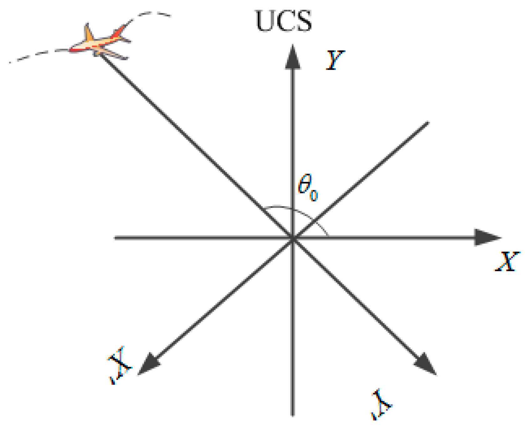
As mentioned above, the imaging result of LOSPI is rotated to the direction of LOS. Therefore, the images in different frames are in different coordinate systems. The ViSAR images are formed in the unified coordinate system (UCS), so all images should be rotated into UCS [3]. As shown in Figure 4, the images in different frames are rotated ${\theta }_0+\pi /2$ clockwise into UCS. The relationship between each coordinate system $\left(x^{\prime },y^{\prime }\right)$ and UCS $\left(x,y\right)$ can be expressed as

$$\left[\begin{array}{l}{x}^{\prime }\\ y^{\prime }\end{array}\right]=\left[\begin{array}{cc}-\sin \left({\theta }_0\right)& \cos \left({\theta }_0\right)\\ -\cos \left({\theta }_0\right)& -\sin \left({\theta }_0\right)\end{array}\right]\left[\begin{array}{l}x\\ y\end{array}\right]$$

(13)

2.2. Resolution and Frame Rate Analysis

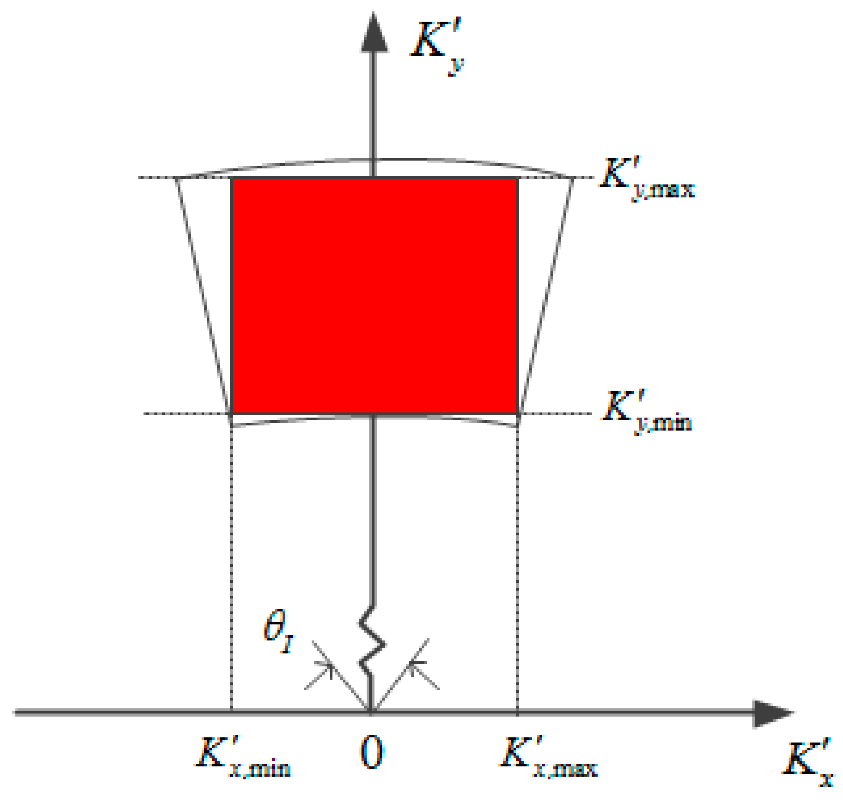
According to SAR imaging theory [36,37,38], the resolution of SAR image is related to the width of wavenumber spectrum. As shown in Figure 5, after LOSPI the range of $K_x^{\prime }$ and $K_y^{\prime }$ can be expressed as

$$\{\begin{array}{l}{K}_x^{\prime }\in \left[K_{x,\min }^{\prime },K_{x,\max }^{\prime }\right]\\ K_y^{\prime }\in \left[K_{y,\min }^{\prime },K_{y,\max }^{\prime }\right]\\ K_{x,\max }^{\prime }=k_c\sin {\varphi }_0\sin \left({\theta }_I/2\right)\\ K_{x,\min }^{\prime }=-k_c\sin {\varphi }_0\sin \left({\theta }_I/2\right)\\ K_{y,\max }^{\prime }=\left(k_c+\Delta k\right)\sin {\varphi }_0\\ K_{x,\min }^{\prime }=\left(k_c-\Delta k\right)\sin {\varphi }_0\end{array}$$

(14)

where $\Delta k=2\pi B/c$ and $B$ is bandwidth, ${\theta }_I$ denotes azimuth integration angle. The expression of range resolution ${\rho }_y$ and azimuth resolution ${\rho }_x$ is

$$\{\begin{array}{l}{\rho }_x=\frac{2\pi }{K_{x,\max }^{\prime }-K_{x,\min }^{\prime }}\\ {\rho }_y=\frac{2\pi }{K_{y,\max }^{\prime }-K_{y,\min }^{\prime }}\end{array}$$

(15)

The expression of Equation (14) is substituted into Equation (15). Due to a small azimuth integration angle that meets the condition of $\sin \left({\theta }_I/2\right)\approx {\theta }_I/2$, the azimuth and range resolution can be rewritten as [38]

$$\{\begin{array}{l}{\rho }_x=\frac{{\lambda }_{\mathrm{c}}\csc {\varphi }_0}{2{\theta }_I}\\ {\rho }_y=\frac{c\csc {\varphi }_0}{2B}\end{array}$$

(16)

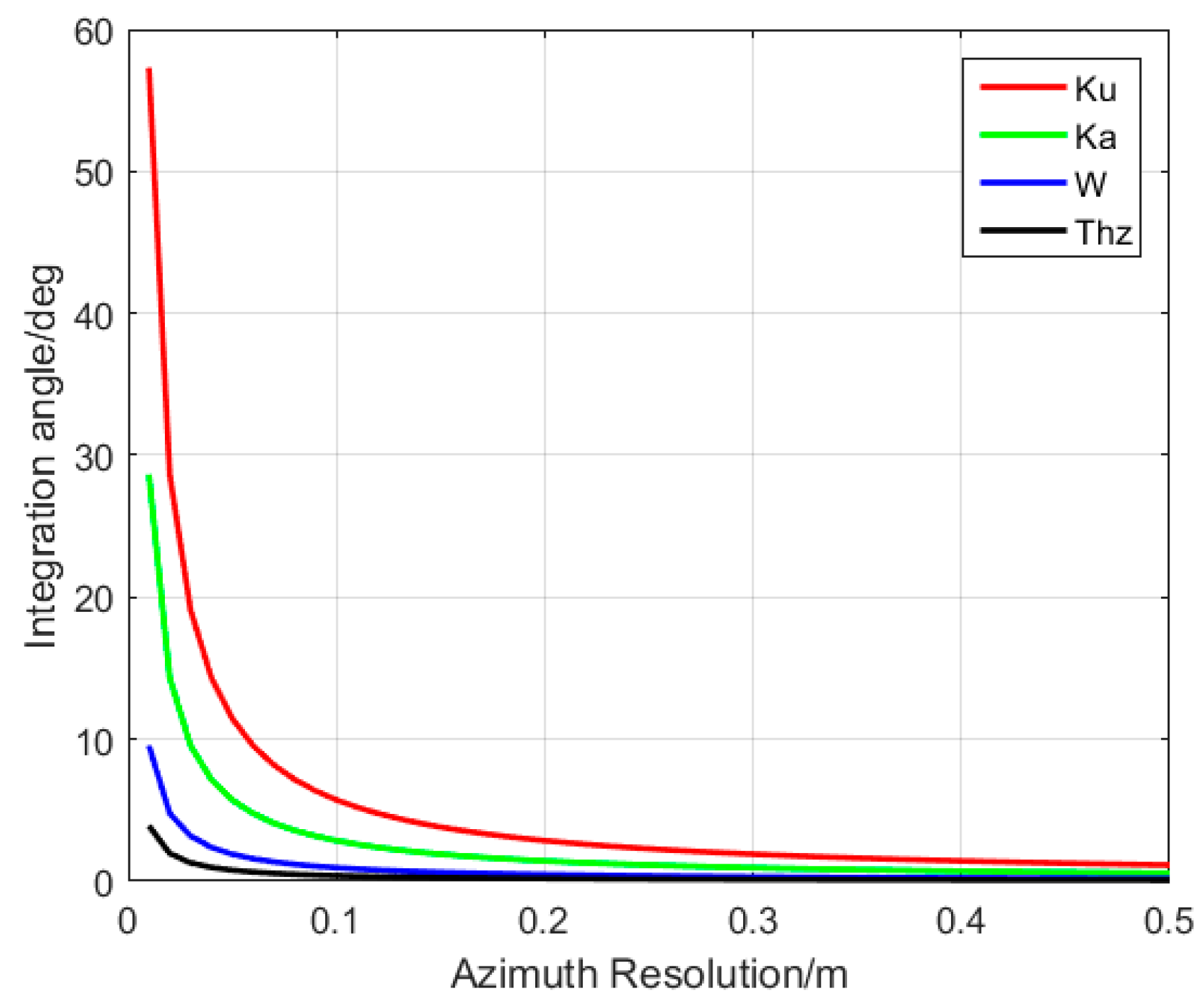
According to Equation (16), the azimuth resolution is inversely proportional to azimuth integration angle. The relationship between the azimuth integration angle and resolution in Ku, Ka, W and THz bands is shown in Figure 6. A given azimuth resolution (high) can be achieved at a smaller azimuth integration angle if the carrier frequency is higher. For PFA, based on a small synthetic aperture angle assumption, we can hardly use low carrier frequency for high resolution imaging.

Assuming the required frame rate of ViSAR is $F_{\mathrm{ps}}$ that can be written as [3,10]

$$F_{\mathrm{ps}}=\frac{2V{\rho }_x}{R_{\mathrm{ref}}c\left(1-\alpha \right)}{f}_c$$

(17)

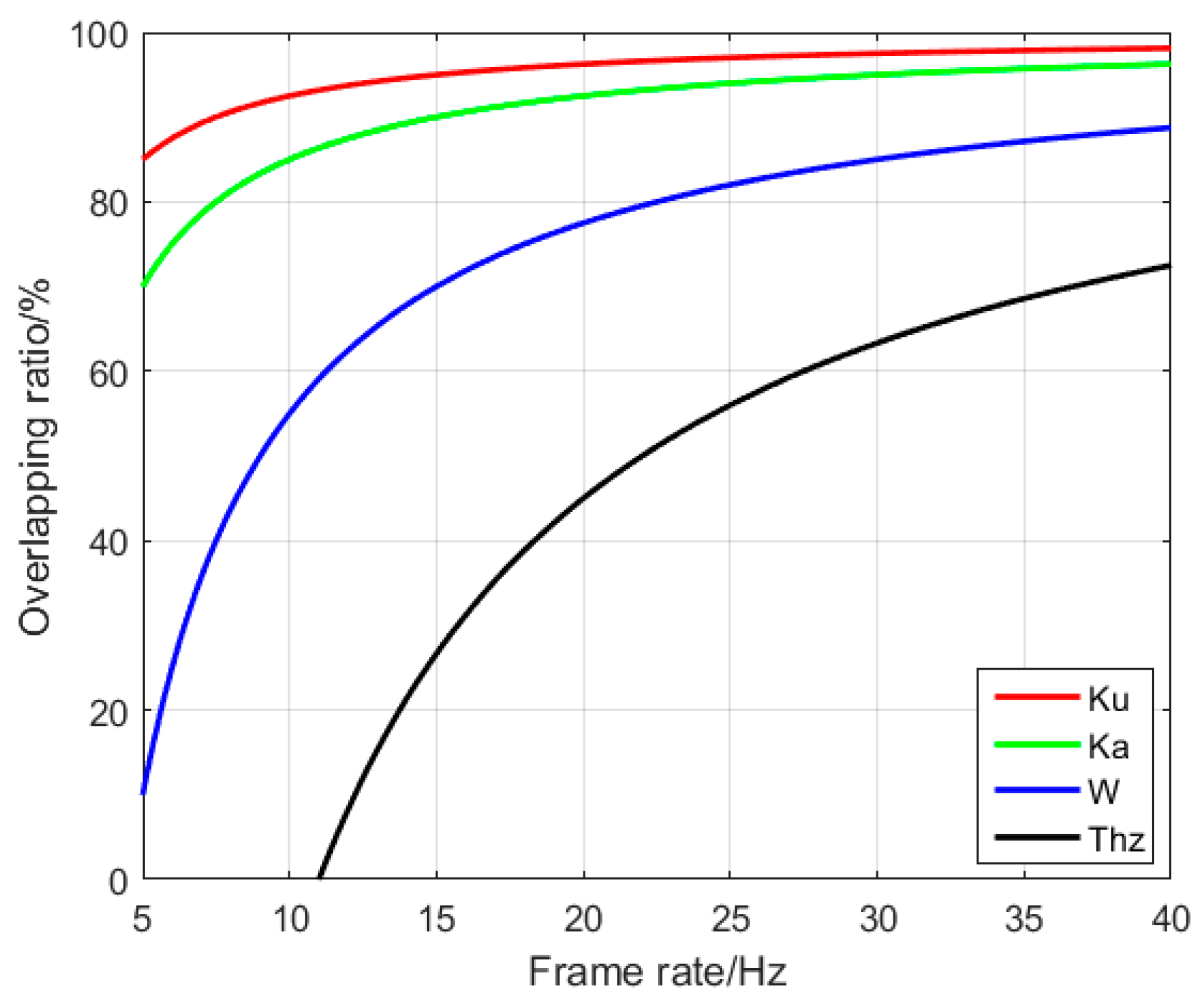
where $\alpha$ denotes sub-aperture overlapping ratio. We set the $R_{\mathrm{ref}}=1200\mathrm{m}$, $V=60\mathrm{m}/\mathrm{s}$ and ${\rho }_x=0.15\mathrm{m}$, then the relationship between overlapping ratio and frame rate is shown in Figure 7. Generally, the frame rate is required to be more than 5 Hz to make ViSAR look more consecutive. For Ku band, the sub-aperture overlapping ratio needs to exceed 80% to meet the frame rate requirements.

2.3. Three-Step Motion Compensation

During the flight of aircraft, the motion error introduced by airflow disturbance and attitude control will seriously affect the SAR image quality. Especially for terahertz band, whose wavelength is short and more sensitive to motion error. Traditional GPS-based MOCO may not satisfy terahertz radar because of limited GPS accuracy. In this paper, a three-step MOCO is proposed that combines GPS-based MOCO and autofocused algorithms [25].

Assuming the actual position of aircraft measured by GPS is $\left(x_{\mathrm{e}},y_{\mathrm{e}},z_{\mathrm{e}}\right)$, the MOCO function can be expressed as

$$H_{\mathrm{MOCO}}=\exp \left[-j\left(k+k_c\right)\left(R_{\mathrm{ref}}-R_{\mathrm{ref}}^{\mathrm{e}}\right)\right]$$

(18)

where $R_{\mathrm{ref}}^{\mathrm{e}}=\sqrt{x_e^2+y_e^2+z_e^2}$ is the actual distance between aircraft and scene center. Multiplying the Equations (6) and (18) can compensate for most motion errors.

$$\begin{array}{ll}S{s}_{\mathrm{e}}\left(k,t_a\right)& =Ss\left(k,t_a\right)·H_{\mathrm{MOCO}}\\ & =A·\mathrm{rect}\left(\frac{k}{2B/c}\right)\times \exp \left[-j\left(k+k_c\right)R_{\mathsf{\Delta }}^{\mathrm{e}}\right]\exp \left[j\phi \left(k,t_a\right)\right]\end{array}$$

(19)

$$\phi \left(k,t_a\right)=\left(k+k_c\right)·\Delta R\left(t_a\right)$$

(20)

where $R_{\Delta }^{\mathrm{e}}=R-R_{\mathrm{ref}}^{\mathrm{e}}$. Due to the very short wavelength of THz Radar and the limitation of GPS precision, after GPS based MOCO there still exists residual phase error and $\phi \left(k,t_a\right)$ denotes the residual phase error, $\Delta R\left(t_a\right)$ denotes the residual motion error. The depression and corresponding azimuth angles can be rewritten as

$$\{\begin{array}{l}\theta =\arctan \left(\frac{y_e}{x_e}\right)\\ {\varphi }_0=\arccos \left(\frac{z_e}{\sqrt{x_e^2+y_e^2+z_e^2}}\right)\end{array}$$

(21)

After LOSPI, the signal can be rewritten as

$$\begin{array}{l}S{s}_e\left(k_x^{\prime },k_y^{\prime }\right)=A·\mathrm{rect}\left(\frac{k}{2B/c}\right)\exp \left[-j\left(k_x^{\prime }{x}_0+k_y^{\prime }{y}_0\right)\right]\times \\ \begin{array}{cc}\begin{array}{cc}\begin{array}{cc}& \end{array}& \end{array}& \end{array} \exp \left[j\phi \left(k_x^{\prime },k_y^{\prime };x_0,y_0\right)\right]\end{array}$$

(22)

According to [39], the properties of phase error along $k_x^{\prime }$ is

$$\eta \left(k_x^{\prime };x_0,y_0\right)=\phi \left(k_x^{\prime },k_c;x_0,y_0\right)$$

(23)

$$\frac{\partial \phi }{\partial k_x^{\prime }}\left(k_x^{\prime },k_y^{\prime };x_0,y_0\right)\approx \frac{\partial \eta }{\partial k_x^{\prime }}\left(k_x^{\prime };x_0,y_0\right)$$

(24)

According to Equation (24), two-dimensional coupled can be neglected, and autofocused algorithm relies on property of phase gradient. What’s more, the spatial variance of phase error can be solved by image segmenting. Because of GPS-based MOCO and short aperture, RCM introduced by phase error can be considered less than range resolution. Therefore, one-dimensional (1D) autofocus can be used to compensate for azimuth phase error. Applying the range FFT, the signal in range-Doppler domain is obtained

$$\begin{array}{ll}{S}_{\mathrm{m}}\left(k_x^{\prime },y\right)& ={\displaystyle \underset{{k^{\prime }}_{y,\min }}{\overset{{k^{\prime }}_{y,\max }}{\int }}S{s}_{\mathrm{e}}\left(k_x^{\prime },k_y^{\prime }\right)}\exp \left(-j{k}_y^{\prime }y\right)d{k}_y^{\prime }\\ & \approx \exp \left[j\eta \left(k_x^{\prime };x_0,y_0\right)\right]\times A·\exp \left(-j{k}_x^{\prime }{x}_0\right)\sin \mathrm{c}\left(\pi \frac{y-y_0}{{\rho }_y}\right)\end{array}$$

(25)

From Equation (25), this model perfectly fits autofocused assumptions. Applying PGA directly can effectively estimate phase error $\eta \left(k_x^{\prime };x_0,y_0\right)$. Let $g\left(m\right)$ represent the expression of Equation (25) at target range cell, $m$ is the azimuth position index.

$$g\left(m\right)=S_m\left(m,y_0\right)=A·\exp \left(-jm{x}_0\right)\exp \left[j\eta \left(m;x_0,y_0\right)\right]\begin{array}{cc}\begin{array}{cc}& \end{array}& 1\le m\le \end{array}M$$

(26)

where $M$ is the length of full aperture.

$$\eta \left(m;x_0,y_0\right)=\angle \left[g\left(m\right)·g^{\ast }\left(m-1\right)\right]$$

(27)

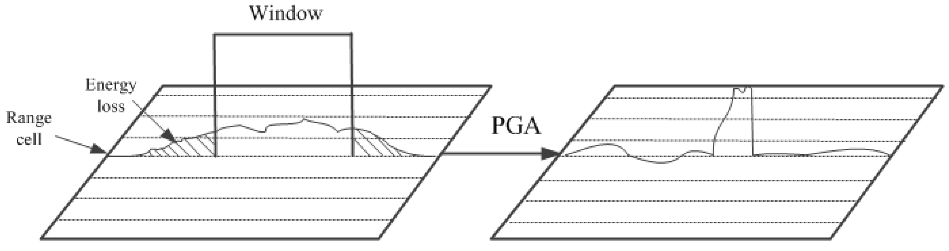
where $\angle [ ]$ is phase angle, $g^{\ast }\left(m\right)$ is the conjugate function of $g\left(m\right)$. The estimator in Equation (27) is well known as PGA [10,16,25]. Unlike the parametric methods PGA estimates the gradient instead of the polynomial coefficients of the phase error function in an optimal manner derived from maximum-likelihood estimation (MLE). In case of very fine azimuth resolution, large squint angle, long standoff distance or low speed radar platform, the PGA may suffer from performance degradation. The underlying mechanism is that the windowing step of PGA, being essentially a low-pass filter, on the one hand improves the signal-to-clutter ratio (SCR) that enhances error estimation accuracy, but on the other hand, it distorts the dominant scatter response that becomes more spread in the presence of significant high-order phase error [29,30]. 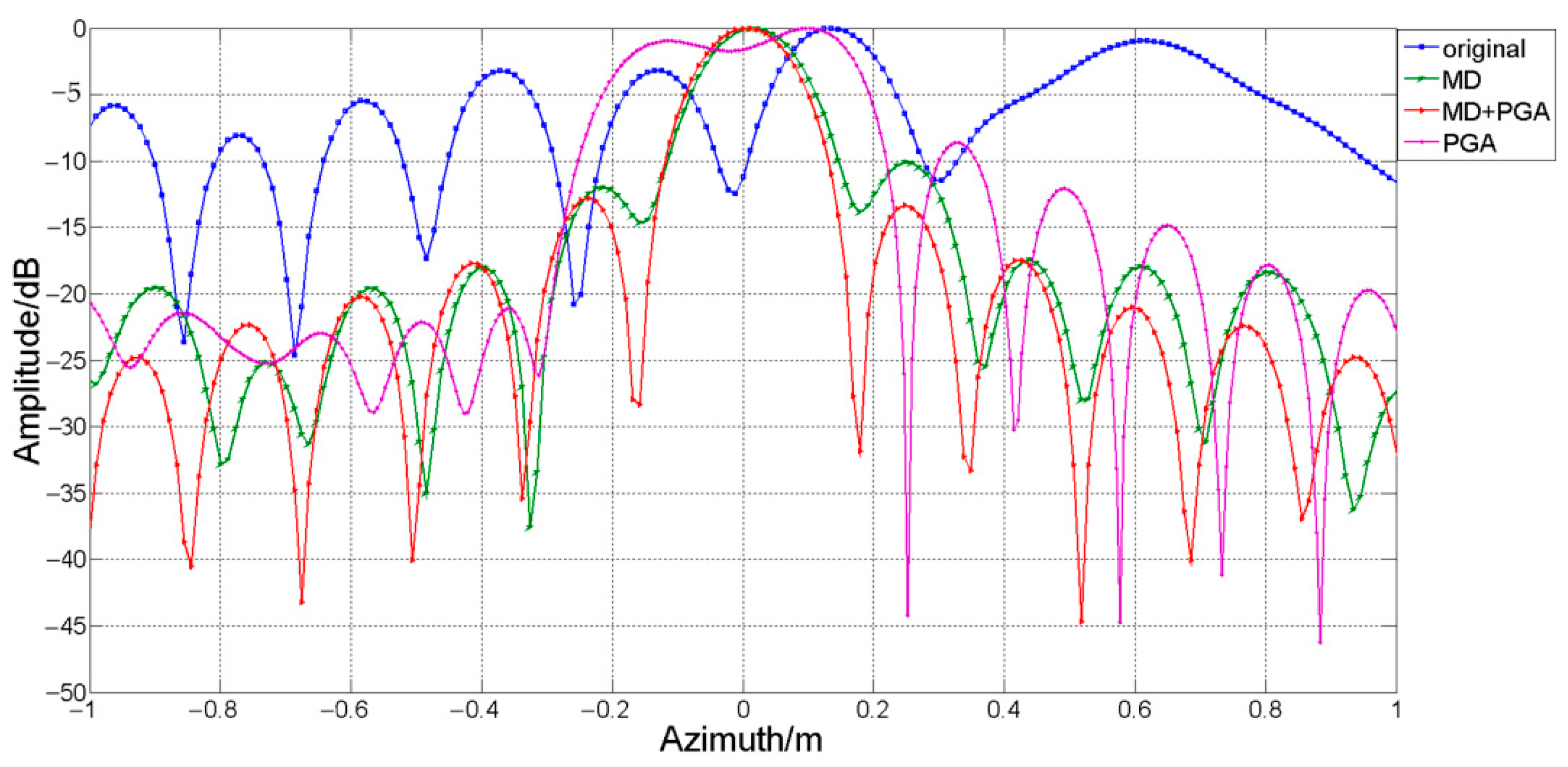As shown in Figure 8, the main lobe widening and energy loss seriously affected the performance of PGA.

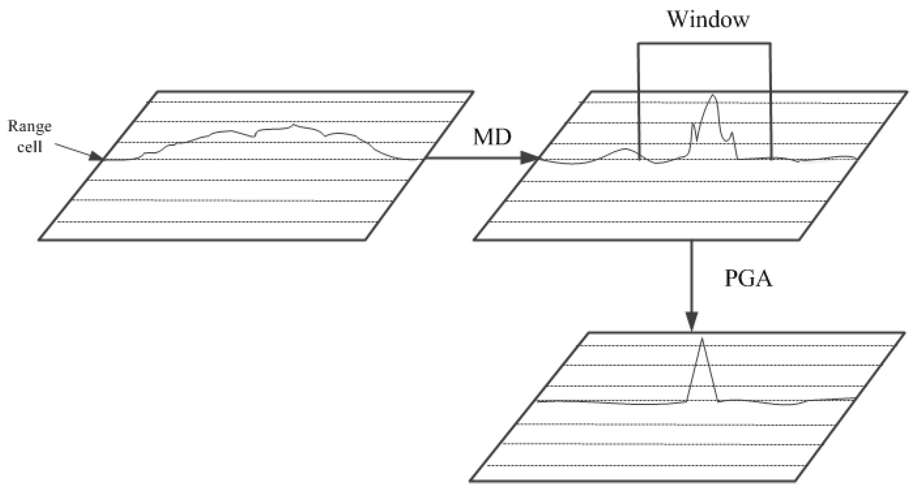
In order to solve the above problem, MD algorithm was applied to compensate for quadratic phase error before PGA. As shown in Figure 9, after MD compensation, main lobe widening and energy loss are effectively suppressed which can greatly improve the performance of PGA.

MD algorithm is one of the autofocus algorithms based on parametric, therefore the spreading of dominant scatter response does not influence the performance of MD [15,25]. For MD algorithm, first, the full aperture is divided into $N$ sub-apertures, the length of each sub-aperture is $m_0$. The phase error within the $n\mathrm{th}$ sub-aperture is

$$\{\begin{array}{l}{g}_n\left(m\right)={\mathrm{rect}}_n\left(m\right)g\left(m\right)\begin{array}{cc}& 1\le n\le N\end{array}\\ {\mathrm{rect}}_n\left(m\right)=\{\begin{array}{l}1\begin{array}{cc},& 1+\left(n-1\right)·m_0\le m\le n·m_0\end{array}\\ 0\begin{array}{cc},& \mathrm{others}\end{array}\end{array}\end{array}$$

(28)

The $n\mathrm{th}$ sub-aperture is evenly divided into two non-overlapping parts $g_1$ and $g_2$, and the offset value ${\delta }_{1,2}$ between $g_1$ and $g_2$ can be given by cross-correlation method.

$${\delta }_{1,2}=\mathrm{corr}\left(g_1,g_2\right)$$

(29)

where $\mathrm{corr}( )$ means cross-correlation. From ${\delta }_{1,2}$, the quadratic phase error can be estimated as

$${\eta }_{2,n}=\frac{4\times PR{F}^2}{{\left(M/N\right)}^2}{\delta }_{1,2}$$

(30)

where ${\eta }_{2,n}$ is the quadratic phase error in $n\mathrm{th}$ sub-aperture. According to Equation (30), the quadratic phase error in each sub-aperture can be obtained. The quadratic phase error of each azimuth cell ${\eta }_2\left(m\right)$ can be obtained by interpolation and then compensate echo signal.

$$\tilde{g}\left(m\right)=g\left(m\right)·\exp \left[-j{\eta }_2\left(m\right)\right]$$

(31)

At last apply PGA to estimate residual high order phase error of $\tilde{g}\left(m\right)$, as shown in Equation (27). After being compensated by MD and PGA, the target is well focused.

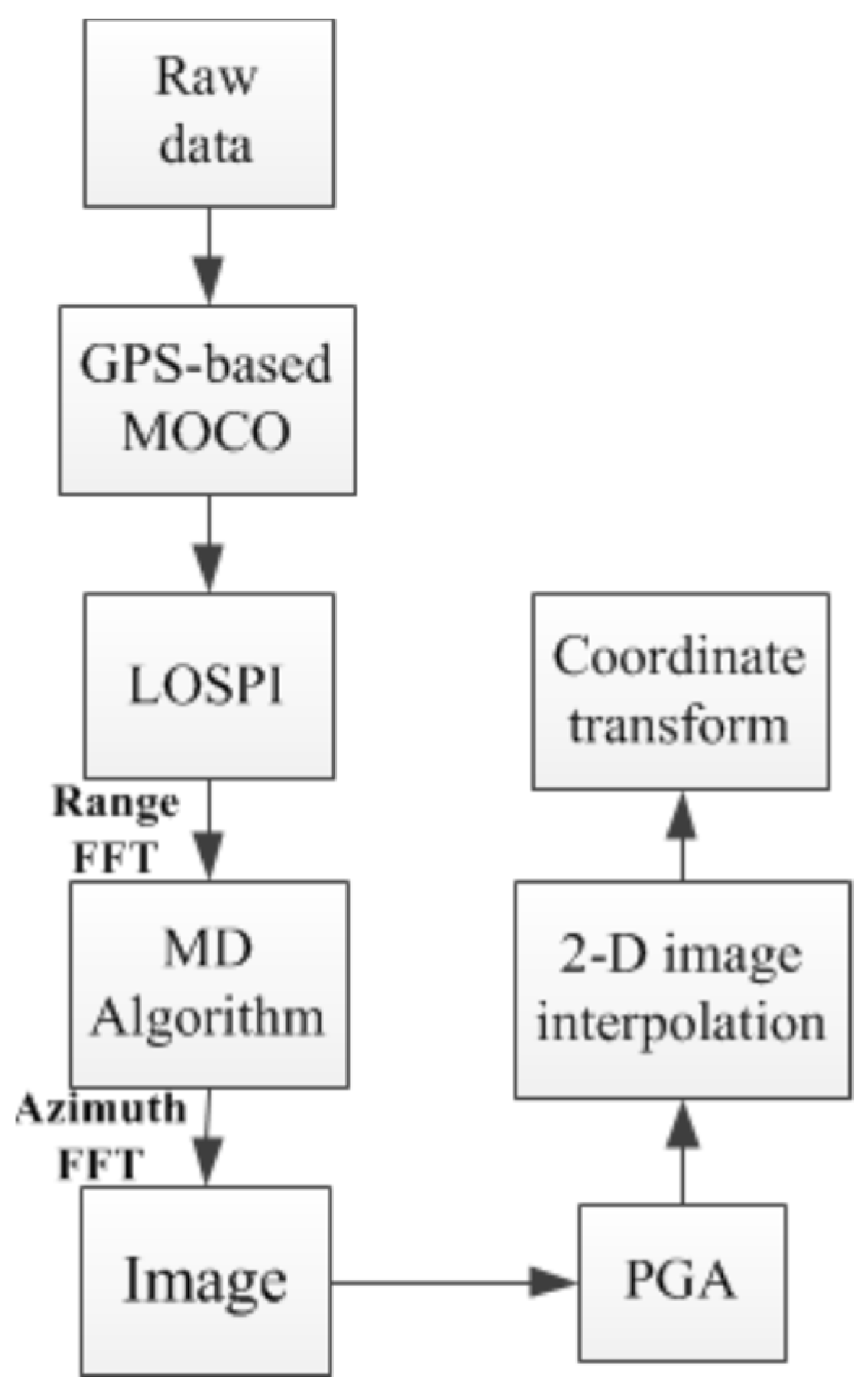
2.4. Complexity Analysis of Proposed Algorithm

To sum up, the proposed imaging algorithm with three-step motion compensation has three main steps: LOSPI, three-step motion compensation and 2D image interpolation. Assuming that the size of input sample in range and slow time are $N_r$ and $N_t$, respectively, the size of the output ROI image is $N_i\times N_i$. A complex multiplication requires four real multiplications and two real additions, a total of six floating point operations (flops). A complex addition requires two real additions, i.e., two flops. A 1-D FFT of length $N$ requires $5N{\log }_{2}N$ flops and a 2D FFT of $N\times N$ requires $10N^2{\log }_{2}N$ flops.

The principle of LOSPI is to convolve the input nonuniform samples onto uniform grid with a truncated Gaussian kernel and exploit 2D FFT for efficient image reconstruction. Assume the length of kernel in the transform is $M_{sp}$. For each grid point, it requires ${\left(2M_{sp}+1\right)}^2$ complex multiplications and ${\left(2M_{sp}+1\right)}^2-1$ complex additions, a total of $8{\left(2M_{sp}+1\right)}^2-2$ flops. Therefore, the computation of the total wavenumber grid is $N_i^2\left[8{\left(2M_{sp}+1\right)}^2-2\right]$ flops.

Three-step motion compensation consists of three procedures. The first procedure is GPS-based MOCO, it requires $N_r\times N_t$ complex multiplication, a total of $6N_r{N}_t$ flops. The second procedure is MD algorithm, it requires $N_i\times N_i$ complex multiplication, a total of $6N_i^2$ flops. The third procedure is PGA algorithm, it requires $N_i^2\left(N_i-1\right)$ complex multiplication, a total of $6N_i^2\left(N_i-1\right)$ flops. The total computation of three-step motion compensation is $6\left[N_r{N}_t+N_i^3\right]$ flops.

The final procedure of 2D image interpolation has the same computation compared with LOSPI. The whole procedure requires a range FFT and an azimuth FFT that transform the wavenumber domain into image domain. The total computation of FFT is $20N_i^2{\log }_2{N}_i$ flops. In summary, the total complexity for the whole procedure is $2N_i^2\left[8{\left(2M_{sp}+1\right)}^2-2\right]+6\left[N_r{N}_t+N_i^3\right]+20N_i^2{\log }_2{N}_i$ flops.

The flowchart of imaging algorithm with three-step motion compensation is shown in Figure 10.

3. Procedures of ViSAR

After all frame images are obtained, there still exist some problems on each frame image such as image shift, low image SNR and non-uniform grey scale between adjacent frame images. These problems seriously affect the quality of ViSAR. In this paper we propose image registration, image denoise and energy balance to improve the quality of ViSAR.

3.1. Image Registration

Due to the motion errors and target height, there is jitter between images. Image registration should be performed first, which is the basis of forming ViSAR. ECC is treated as a performance criterion for the image registration problem [40,41].

3.2. Image Denoise

To improve the image SNR, there are several methods that could be used such as spatial filtering algorithm and transform domain filtering algorithm. Compared with spatial filtering algorithm, transform domain filtering algorithm enhances the ability of preserving the detail structure and has high computational efficiency. Lee filter and non-subsample shearlet transform (NSST) [42,43] are the typical methods of spatial filtering algorithm and transform domain filtering algorithm respectively. Figure 11 shows the results of Lee filter and NSST. There are several indexes which can assess the performance of each method. For the image of size $N\times N$, assume the filter window is $M\times M$, the complexity analysis of two methods is shown in

Table 1. Complexity analysis of different filtering algorithm.

	Complex Addition	Complex Multiplication	Total
Lee Filter	$N^2\left(M^2+2\right)$	$3N^2$	$5N^2+N^2{M}^2$
NSST	$4N^2$	$N^2$	$5N^2$

.

Edge preserved index (EPI) [44] is a measure to assess the edge-preservation capacity of the filters. The expression of EPI is defined as

$$\mathrm{EPI}=\frac{{\displaystyle \sum _{i=1}^n\left|{\widehat{x}}_{i,1}-{\widehat{x}}_{i,2}\right|}}{{\displaystyle \sum _{i=1}^n\left|x_{i,1}-x_{i,2}\right|}}$$

(32)

where $x_{i,1}$, $x_{i,2}$, ${\widehat{x}}_{i,1}$ and ${\widehat{x}}_{i,2}$ are the values of the reference and filtered images, respectively, observed on the one-pixel wide lines on both sides of the edge. Larger values correspond to a better edge retaining ability of the filter. Signal-to noise ratio (SNR) [44] reflects the quality of filtered images and larger values correspond to a better quality. The expression of SNR is defined as

$$\mathrm{SNR}\left(x,\widehat{x}\right)=10{\log }_{10}\frac{\mathrm{Var}\left(x\right)}{\mathrm{E}\left[{\left(x-\widehat{x}\right)}^2\right]}$$

(33)

where $x$ and $\widehat{x}$ reflect reference and filtered images, respectively. $E[.]$ denotes statistical mean, $\mathrm{Var}(.)$ denotes statistical variance.

According to

Table 2. Measured parameters of different filtering algorithm.

	Time (s)	EPI	MSE
Lee Filter	48.96	0.24	55.42
NSST	3.70	0.52	40.68

, NSST has a higher performance which is more suitable to apply in image denoise.

3.3. Energy Balance

To uniform the brightness of different images, histogram transfer algorithm is applied [45]. Firstly, the transfer map is calculated according to grey histogram of the reference image. Secondly, according to the transfer map, the original image is mapped onto the histogram of the reference image. As shown in Figure 12, Figure 12a is the reference image and Figure 12b is the original image, and after the histogram transfer, the grey scale of Figure 12c is uniformed to Figure 12a. The grey scale histograms of Figure 12a–c are shown in Figure 13a–c, respectively.

In addition to generating ViSAR, all aspects of SAR images can be fused in one image after histogram transfer algorithm. Compared with a single SAR image, the image fusion result can not only improve image signal-to noise ratio but also solve shadow occlusion issues that arise from the typical side-looking geometry [1]. Therefore, the image fusion result is always used in SAR image interpretation. In image fusion, each pixel $f\left(x,y\right)$ represents the mean backscatter result of the generated image stack as

$$f\left(x,y\right)=\frac{{\displaystyle {\sum }_n{I}_n\left(x,y\right)}}{N}$$

(34)

where $N$ is the total number of frame images, $I_n\left(x,y\right)$ is the intensity of each image’s pixel. The flowchart of forming ViSAR and image fusion is shown in Figure 14.

4. Experiment and Analysis

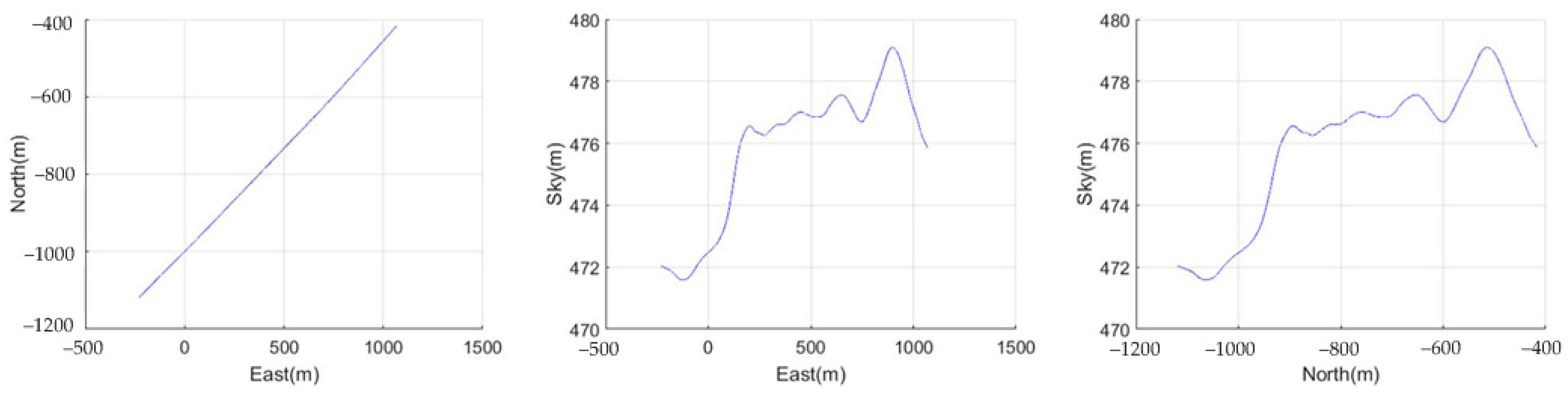
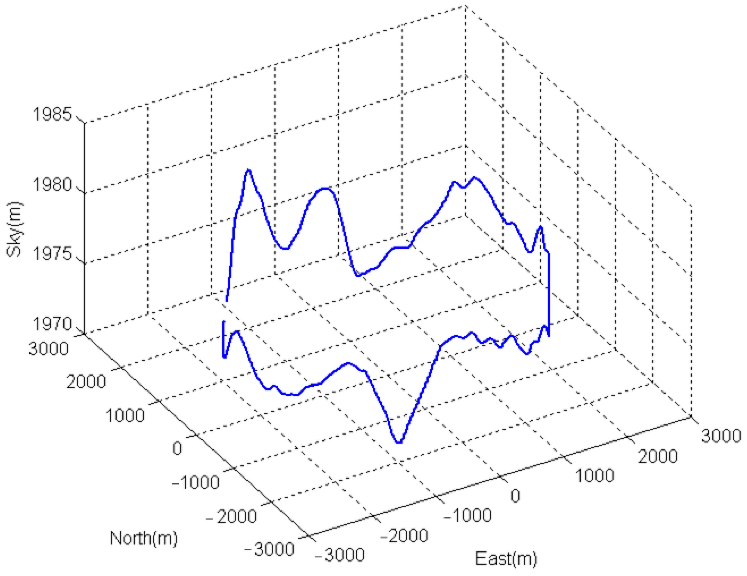
In order to demonstrate the theoretical analysis presented in this paper further, an experimental data processing experiment was carried out. The THz experiment was carried out by Beijing Institute of Radio Measurement in Shaanxi province, China. The radar operated in THz band. Figure 15 shows the flight trajectory of radar platform, which is not ideal linear trajectory. Because of terahertz band, the motion error cannot be neglected. The experimental scene is shown in Figure 16. There were three groups of trihedral corner reflectors and an aircraft in the scene. The aircraft flew from east to west. The size of experimental size is $200\mathrm{m}\times 200\mathrm{m}$. Our experimental data processing was based on the Intel i7-4790 CPU, AMD Radeon R7 350 GPU hardware platform.

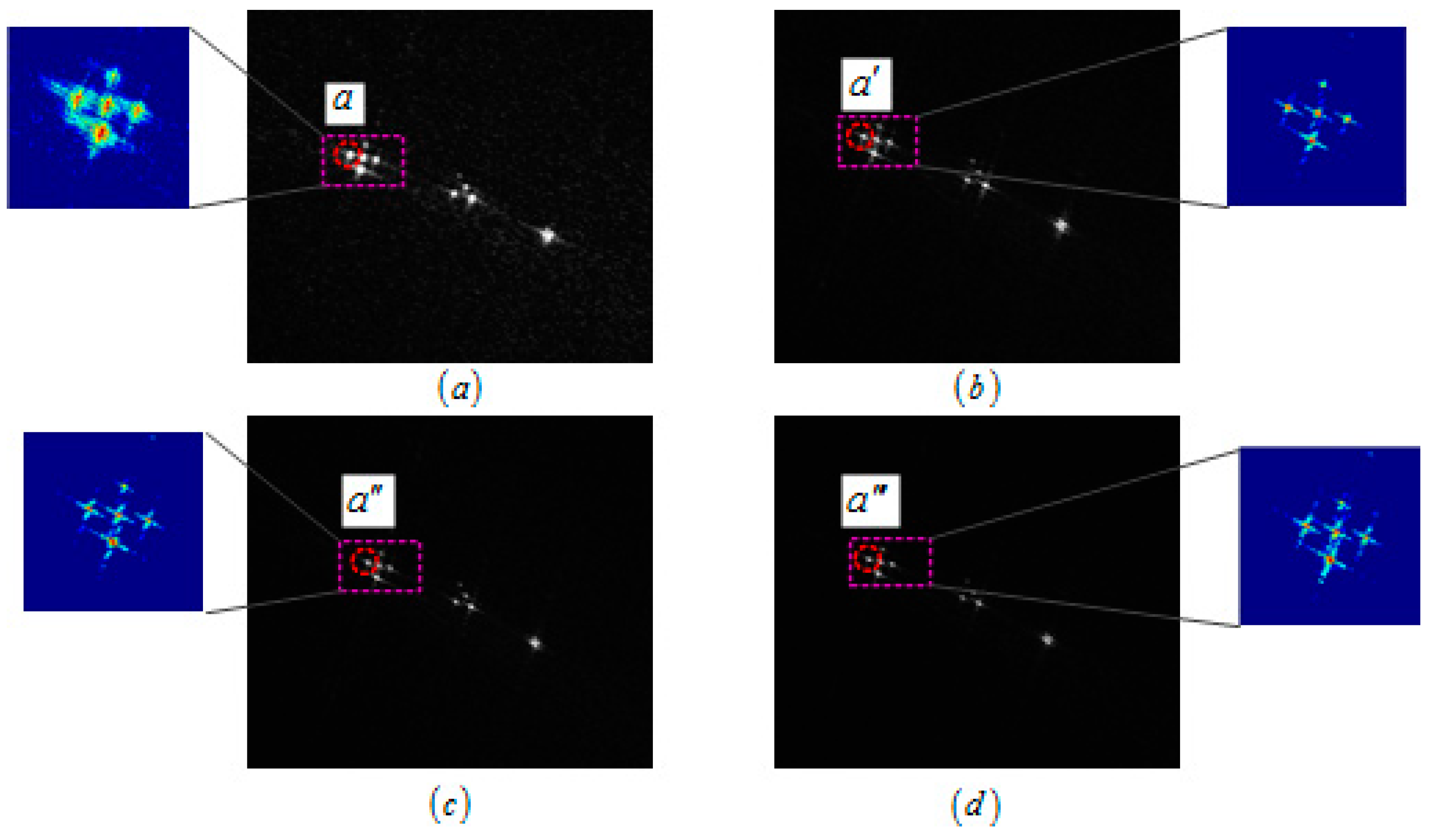
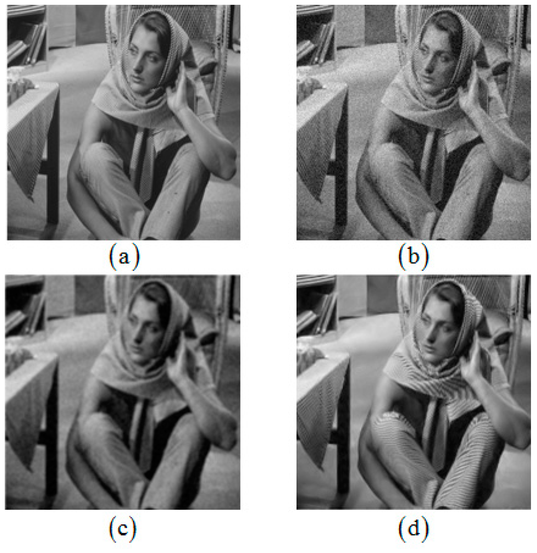
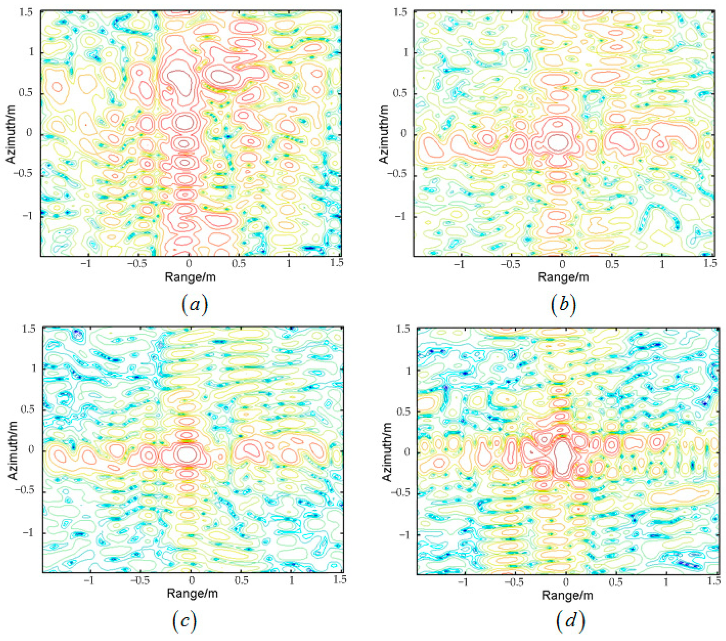
The azimuth integration angle was ${0.2}^{\mathsf{o}}$, resulting in 0.15 m azimuth resolution. To achieve 15 Hz frame rate, the overlapping ratio can be set 26%. According to (11), the DOF $r$ was 283 m, which is much larger than experimental size, therefore the image defocused, introduced by planar wave approximation, was neglected. To verify the effectiveness of three-step MOCO, we selected an imaging result of a single frame as shown in Figure 17. In order to compare visibility, four same position targets $a$, $a^{\prime }$, $a^{″}$ and $a^{‴}$ were selected to be compared, and the contour map results are shown in Figure 18. Point $a$ seriously defocused along azimuth. It revealed that the motion error greatly impacted the focusing properties. Compared with point $a$, point $a^{\prime }$ was refocused by MD, which the main lobe focused well. However, the residual high order phase error caused the asymmetrical distribution of the side lobe. Point $a^{″}$ was processed by MD and PGA, and we can see that the main lobe was well focused and the side lobe was symmetrically distributed. As mentioned before, main lobe widening and energy loss seriously affect the performance of PGA, therefore point $a^{‴}$ which was processed by PGA directly is not focused as well as point $a^{″}$. The azimuth profile of point $a$, $a^{\prime }$, $a^{″}$ and $a^{‴}$ are shown in Figure 19.

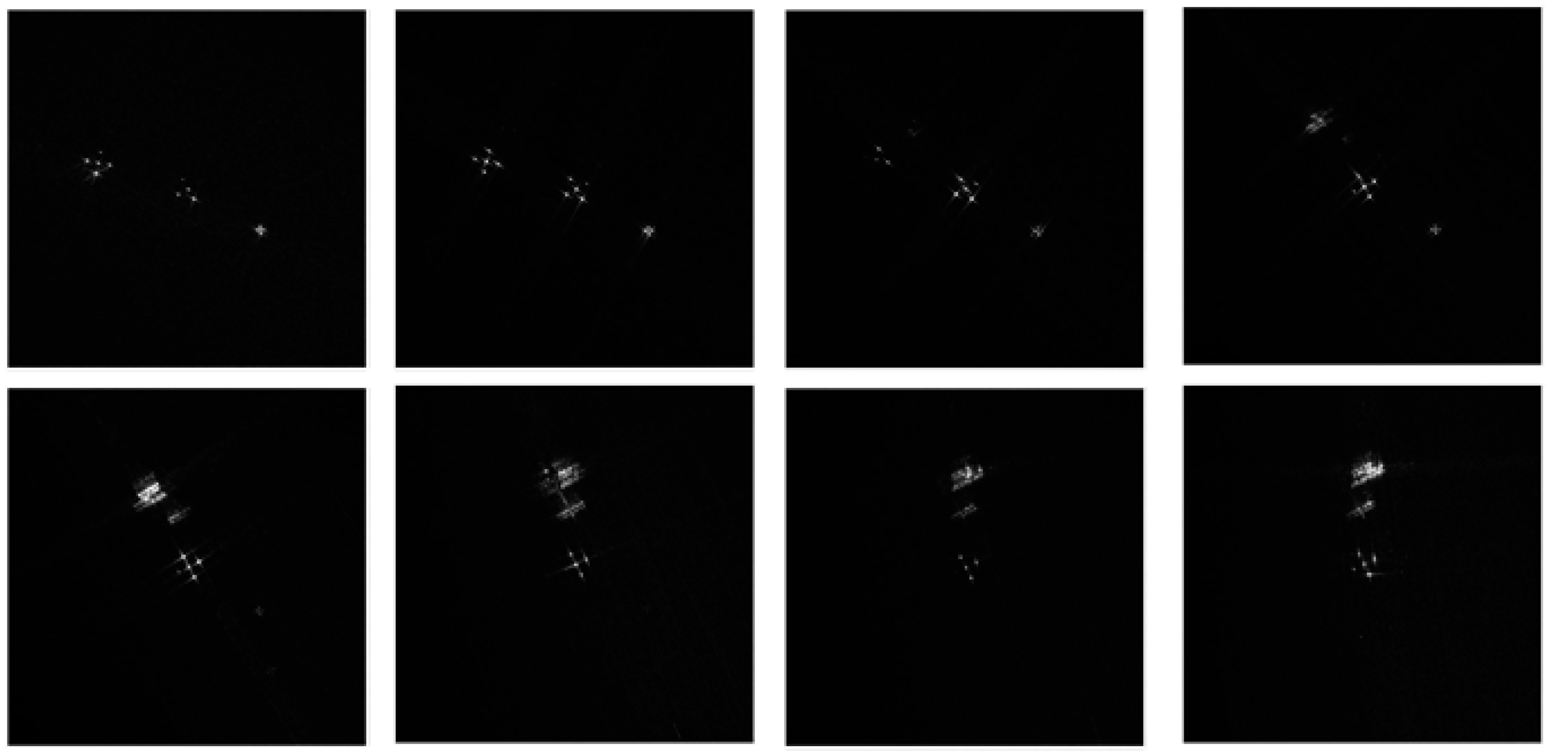
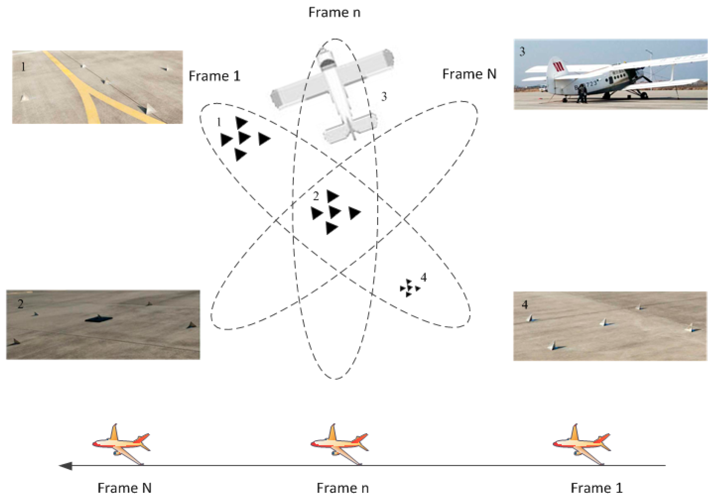
Furthermore, to verify the effectiveness of ViSAR procedures that were proposed in this paper, imaging results of different frames are shown in Figure 20. According to imaging results, there was no jitter and grey scale difference between different frame images. To illustrate the whole imaging scene, the multiple-frame images were fused together. The result is shown in Figure 21. Because of the high resolution in terahertz band, the outline of the aircraft is quite clear in the fused image.

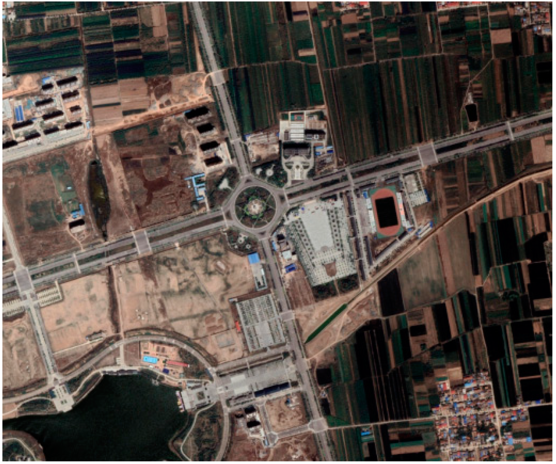
To verify the ability of the long-time persistent surveillance of ROI, another experiment was carried out by National University of Defense Technology in Shaanxi province, China. The carrier frequency of radar was Ku band. The size of the experimental scene was $800\mathrm{m}\times 800\mathrm{m}$, and the experimental scene from Google Earth is shown in Figure 22. Figure 23 shows the 3D flight trajectory. Compared with linear spotlight SAR, circular SAR (CSAR) can illuminate the targets for long time which can achieve long-time persistent surveillance.

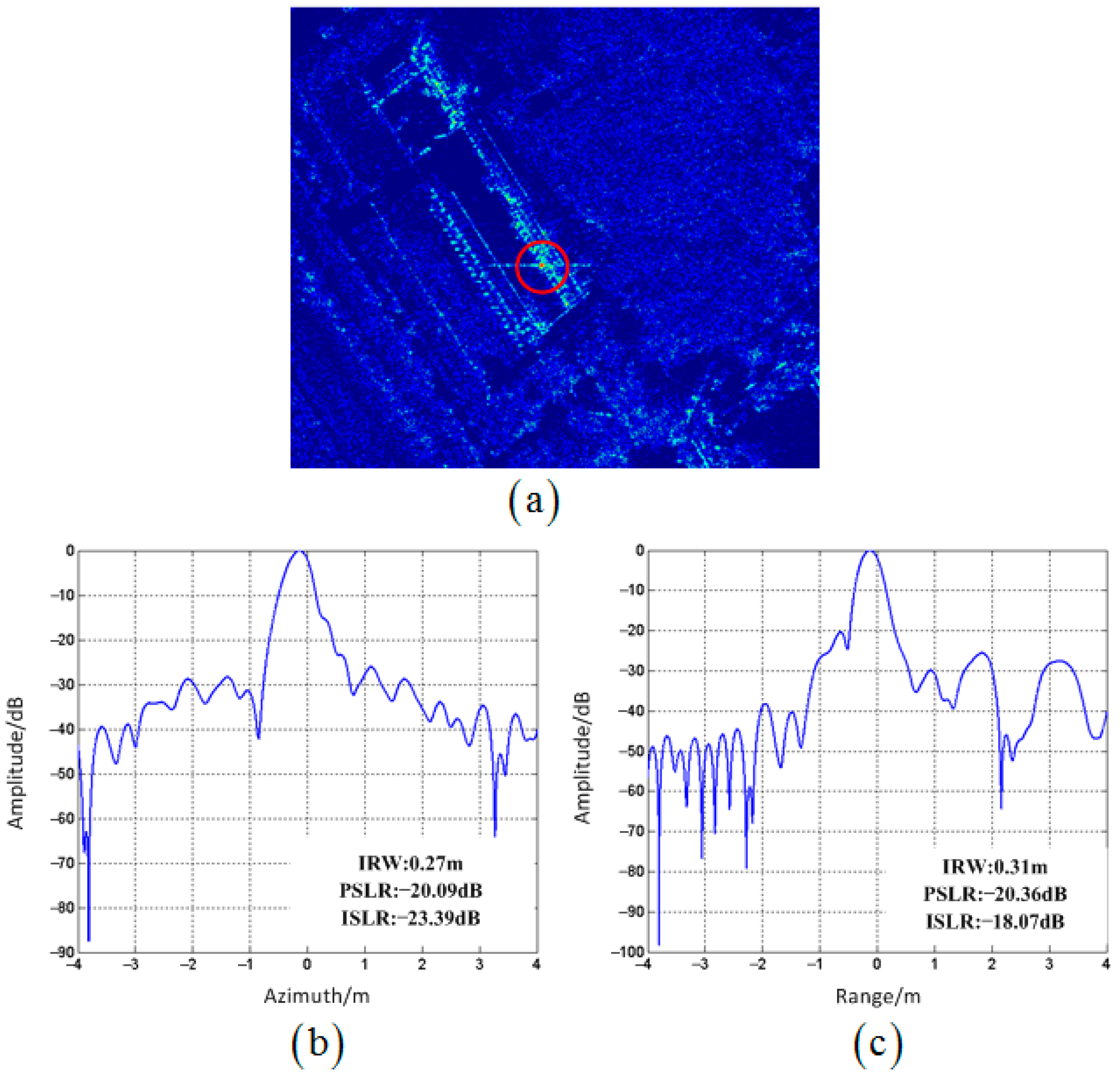
According to (16), each frame image has an approximate illumination time of 2 s corresponding to ${2.2}^{\circ }$ azimuth integration angle and thus 0.25 m resolution in azimuth and 0.30 m resolution in range. To obtain results in good and smooth videos, the frame rate required 10 Hz with an overlap of 80%. This lead to approximate 1000 sub-aperture SAR images for a full circle. In Figure 24, a target point is selected to analyze the imaging performance. The azimuth/range profiles and the measured parameters of target point are presented in Figure 24b,c, respectively. We can see that the target focused well, which further proved the effectiveness of three-step MOCO.

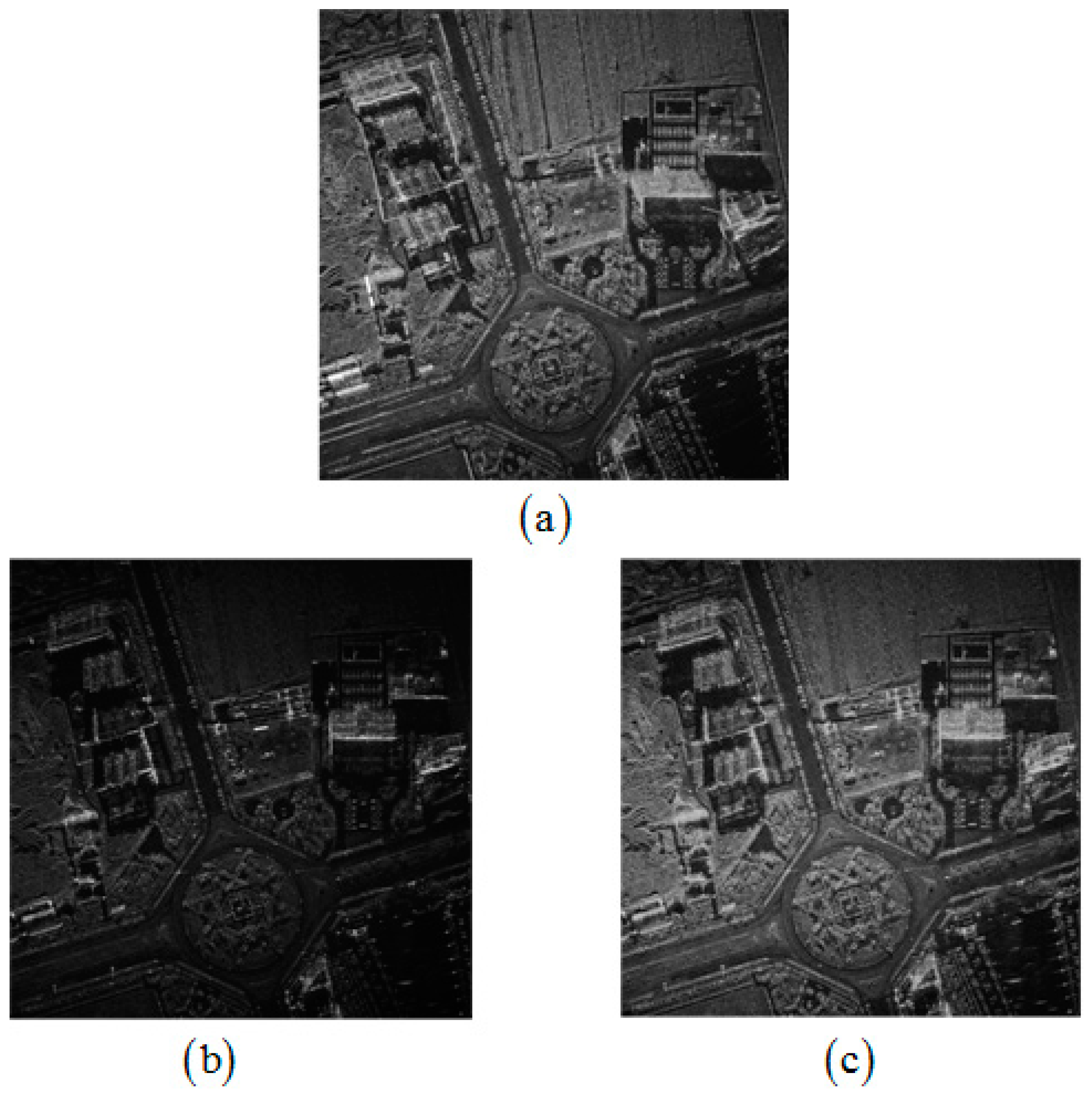
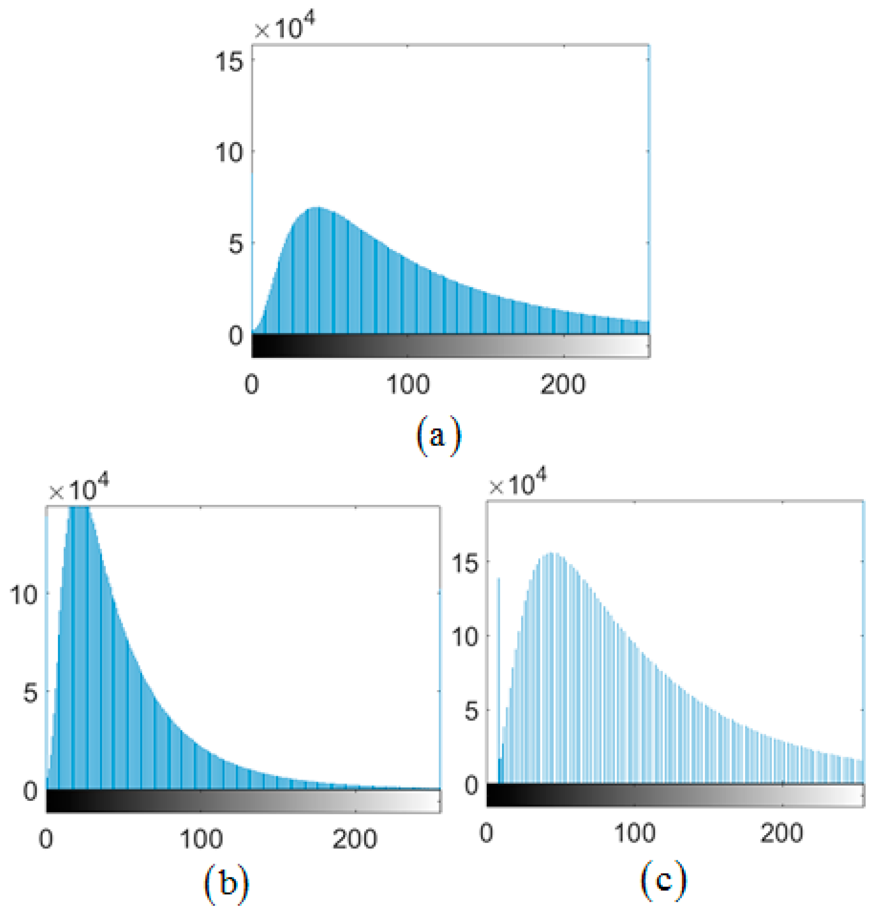
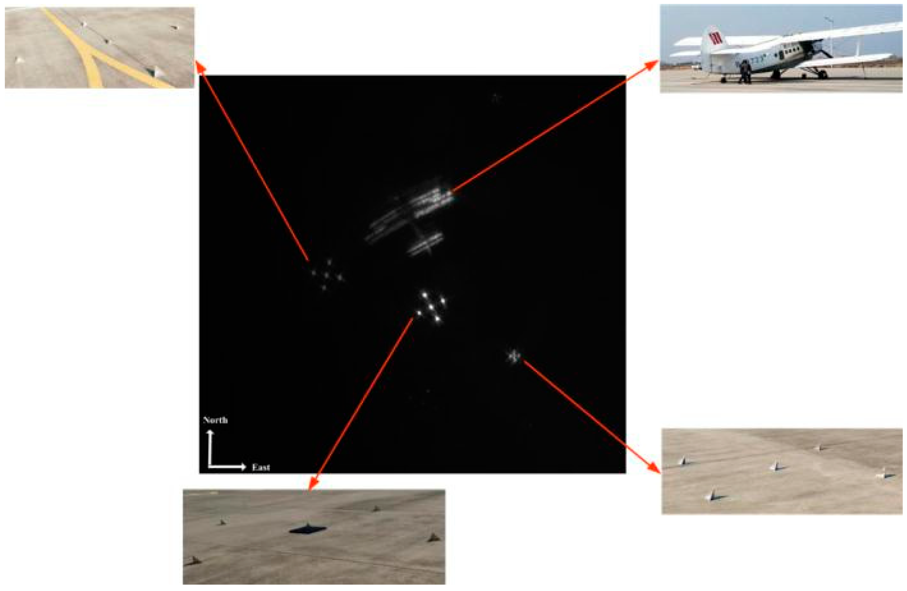
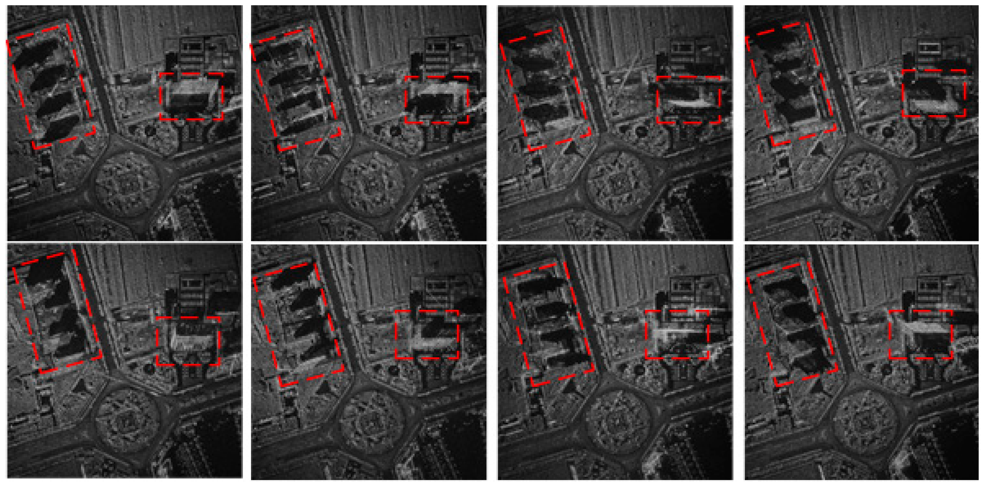
After all frame images were processed by ViSAR procedures, the ViSAR could be obtained. It shows eight frame images from different azimuth angles in Figure 25. There are three residential buildings located in the northwest and a commercial building in northeast which are marked with red rectangles. Noticeably, the large shadow formation of buildings covers different large space of images in different azimuth angles. Objects behind the buildings remain hidden to the observer. The same is true for objects in front of the building (in the LOS direction to the radar), because of the large foreshortening of the building.

The capability of detecting and tracking the moving targets is presented in Figure 26. The images were chosen in the consecutive order in a slightly interval time to better represent the dynamics of the scene. In total, the illustrated scene comprised of interval time 18 s, corresponding to integration angle ${19.8}^{\circ }$. Due to shadows formed by moving vehicles that can show a clear contrast compared to ground clutter, we can track the vehicles easily. For tracking vehicles, the quality of shadow is an important factor. While the vehicle was moving, the duration time that the parts of area covered with shadow during the total sub-aperture time determine the quality of the shadow [46]. If the car is going fast or sub-aperture time is long, the shadow may smear and be buried in ground clutter [46].

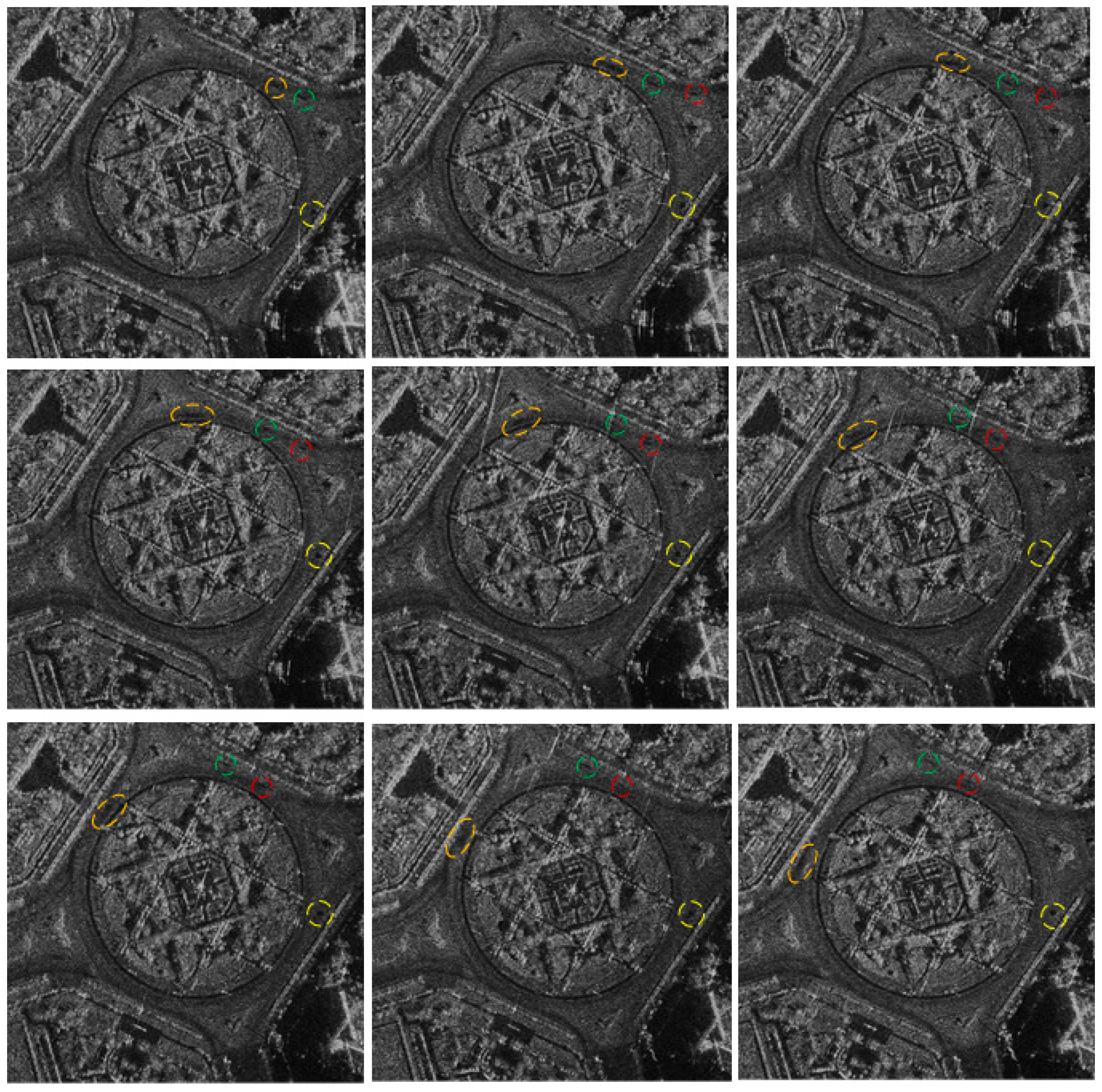
In Figure 26, some vehicles are marked by different colors to better track their trajectories. From left to right then from up to down, it can be seen that the vehicle marked by orange ellipse was heading west along ring road very fast while the vehicles marked by green and red circle were heading north. Meanwhile a vehicle marked by yellow was going to east very slow.

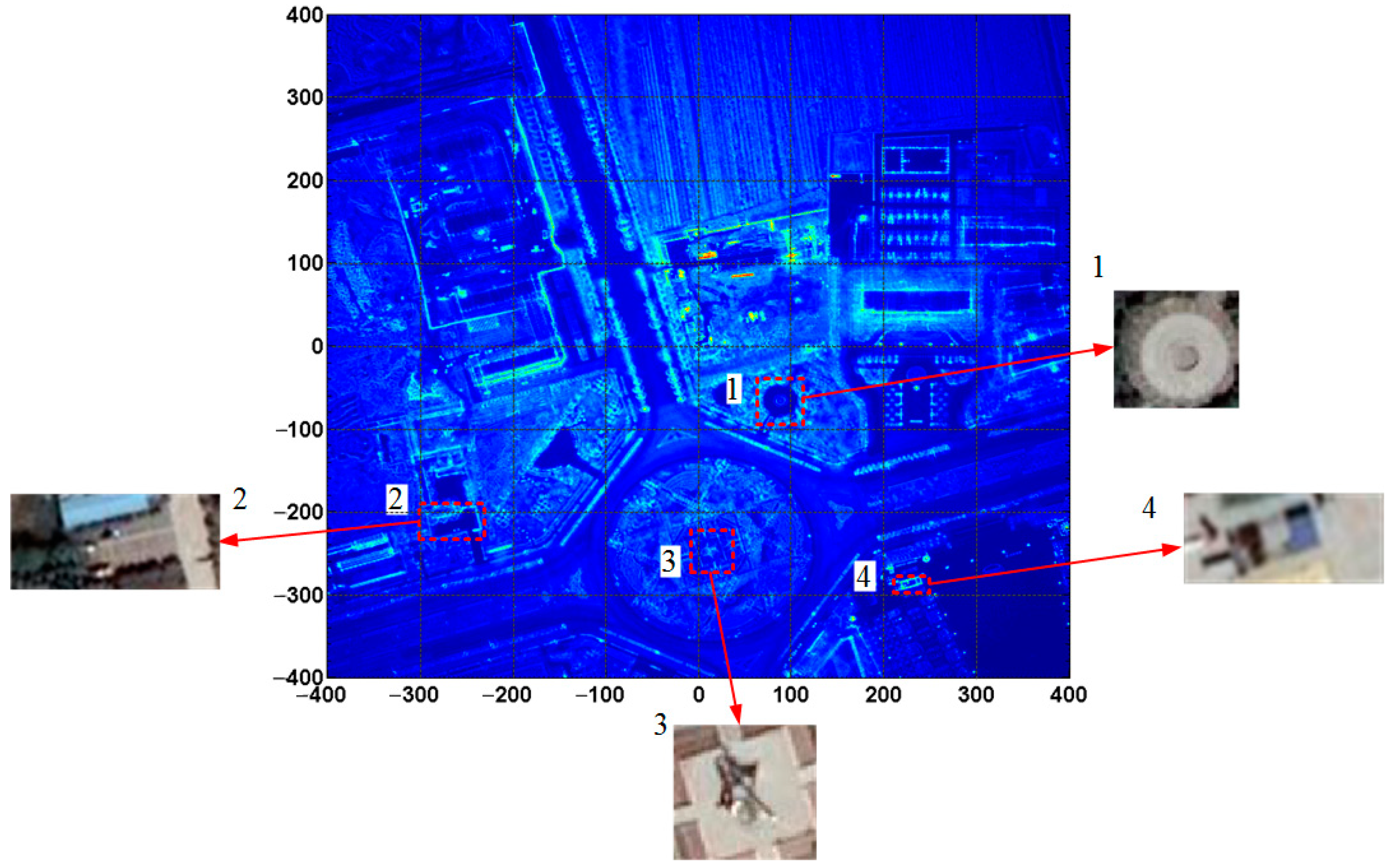
The image fusion result is shown in Figure 27. Compared with signal aspect image, the fusion result solves the shadow occlusion problem which can be used in the following SAR image interpretation. In order to compare the estimated position of the targets based on fused image with the true position of targets, we selected four areas as shown in Figure 27, and the corresponding zoom-in optical images are shown in Figure 27. The imaging center was set as the origin of the coordinate system, therefore the coordinates of the regional center could be obtained. For the true position of the regional center, we can obtain them from Google Maps. In fusion image, the coordinates of each region 1, 2, 3 and 4 are $\left(89.0,-66.1\right)$, $\left(-258.3,-214.4\right)$, $\left(13.8,-248.4\right)$ and $\left(229.0,-285.4\right)$, respectively. From Google Maps, the true positions of each regional center are $\left(89.5,-66.0\right)$, $\left(-259.5,-214.2\right)$, $\left(12.9,-248.0\right)$ and $\left(230.3,-286.1\right)$, respectively. By comparison, the position of targets in fusion result corresponds to the true position.

5. Conclusions

In this paper, a ViSAR imaging algorithm based on three-step MOCO was proposed, which could effectively solve the image defocused introduced by motion error. Furthermore, procedure of ViSAR was proposed that contains several image processing methods that greatly solved jitter, non-uniform grey scale and low image SNR between different aspect images. Then, we analytically derived up the relationship between azimuth integration angle and resolution in different carrier frequency. For given resolution, as carrier frequency becomes higher, a shorter integration angle is needed. We further analyzed the relationship between frame rate and sub-aperture overlapping ratio. For given frame rate, as carrier frequency becomes higher, a lower overlapping ratio is needed. The experiment results showed the great potential of THz band in ViSAR. The results demonstrated that only a small integration angle can achieve high resolution, and low overlapping ratio can achieve high frame rate ViSAR. We further demonstrated the capability of long-time observing urban scenes in Ku band. From the ViSAR result in Ku band, we could see that the observation of multiple moving targets in single-channel data was feasible. The results on data fusion of multiple aspect images were presented and demonstrate the benefit from this geometry. The covering of objects beside large buildings can be reduced.